Shear stress relaxation and ensemble transformation
of shear stress autocorrelation functions revisited

Abstract

We revisit the relation between the shear stress relaxation modulus $G(t)$, computed at finite shear strain $0<\gamma\ll 1$, and the shear stress autocorrelation functions $C(t)|_{\gamma}$ and $C(t)|_{\tau}$ computed, respectively, at imposed strain $\gamma$ and mean stress $\tau$. Focusing on permanent isotropic spring networks it is shown theoretically and computationally that in general $G(t)=C(t)|_{\tau}=C(t)|_{\gamma}+G_{\mathrm{eq}}$ for $t>0$ with $G_{\mathrm{eq}}$ being the static equilibrium shear modulus. $G(t)$ and $C(t)|_{\gamma}$ thus must become different for solids and it is impossible to obtain $G_{\mathrm{eq}}$ alone from $C(t)|_{\gamma}$ as often assumed. We comment briefly on self-assembled transient networks where $G_{\mathrm{eq}}(f)$ must vanish for a finite scission-recombination frequency $f$. We argue that $G(t)=C(t)|_{\tau}=C(t)|_{\gamma}$ should reveal an intermediate plateau set by the shear modulus $G_{\mathrm{eq}}(f=0)$ of the quenched network.

I Introduction

Shear stress relaxation.

The static equilibrium shear modulus $G_{\mathrm{eq}}$ Landau and Lifshitz (1959); Rubinstein and Colby (2003); Doi and Edwards (1986); Hansen and McDonald (2006); Götze (2009); Alexander (1998); Witten and Pincus (2004) is an important order parameter Callen (1985); Chandler (1987); Chaikin and Lubensky (1995) characterizing the transition from the liquid/sol ($G_{\mathrm{eq}}=0$) to the solid/gel state ($G_{\mathrm{eq}}>0)$ where the particle permutation symmetry of the liquid state is lost for the time window probed Alexander (1998); Witten and Pincus (2004). Examples of current interest for the determination of $G_{\mathrm{eq}}$ include crystalline solids Sausset et al. (2010), glass-forming liquids and amorphous solids Götze (2009); Barrat et al. (1988); Wittmer et al. (2002); Tanguy et al. (2002); Berthier et al. (2005, 2007); Yoshino and Mézard (2010); Szamel and Flenner (2011); Schnell et al. (2011); Yoshino (2012); Klix et al. (2012); Xu et al. (2012); Wittmer et al. (2013a, b); Zaccone and Terentjev (2013); Ozawa et al. (2012); Mizuno et al. (2013), colloidal gels del Gado and Kob (2008), permanent polymeric networks Rubinstein and Colby (2003); Duering et al. (1991, 1994); Ulrich et al. (2006), hyperbranched polymer chains with sticky end-groups Tonhauser et al. (2010) or networks of telechelic polymers Zilman et al. (2003). As emphasized by the thin horizontal line in Fig. 1, the shear modulus of an isotropic solid may be determined experimentally from the long-time limit Rubinstein and Colby (2003); foo (a)

$$G_{\mathrm{eq}}\equiv\lim_{t\to\infty}G(t)$$ (1)

of the shear stress relaxation modulus (bold solid line) defined as $G(t)\equiv\delta\tau(t)/\gamma$. It measures the stress increment $\delta\tau(t)=\left<\hat{\tau}(t)-\hat{\tau}(0^{-})\right>$ due to a step strain $0<\gamma\ll 1$ imposed at time $t=0$. Here $\hat{\tau}(t)$ denotes the instantaneous shear stress which may be measured experimentally from the forces acting on the walls of the shear cell Rubinstein and Colby (2003).

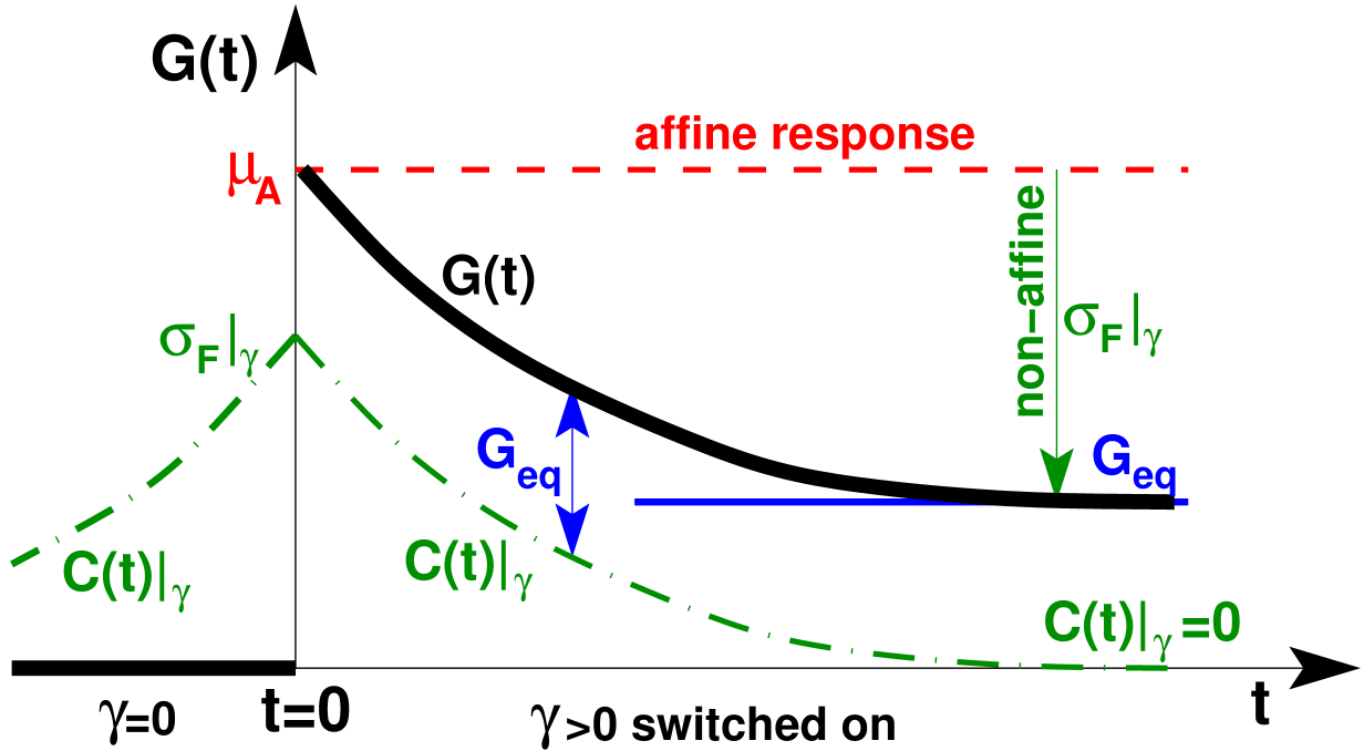
Figure 1: Schematic comparison of the shear relaxation modulus $G(t)$ (bold solid line) and the shear stress autocorrelation function $C(t)|_{\gamma}$ computed in the $\text{NV}\gamma\text{T}$-ensemble (dash-dotted line). Note that $G(0^{+})=\mu_{\mathrm{A}}=\sigma_{\mathrm{F}}|_{\tau}$ and $C(0)|_{\gamma}=\sigma_{\mathrm{F}}|_{\gamma}$ with $\mu_{\mathrm{A}}$ being the affine Born-Lamé contribution to the shear modulus $G_{\mathrm{eq}}=\mu_{\mathrm{A}}-\sigma_{\mathrm{F}}|_{\gamma}$ with $\sigma_{\mathrm{F}}\equiv\beta V\langle\delta\hat{\tau}^{2}\rangle$ characterizing the static shear stress fluctuations Barrat et al. (1988); Parrinello and Rahman (1982); Lutsko (1989); Tanguy et al. (2002); Yoshino and Mézard (2010); Wittmer et al. (2013a).

Correlation functions.

A quantity related to $G(t)$ is the shear stress autocorrelation function Hansen and McDonald (2006); Götze (2009)

$$C(t)\equiv\beta V\left<\delta\hat{\tau}(t)\delta\hat{\tau}(0)\right>\equiv\tilde{C}(t)-\beta V\langle\hat{\tau}\rangle^{2}$$ (2)

with $\beta=1/\mbox{$k_{\rm B}T$}$ being the inverse temperature and $V$ the volume. We write $C(t)|_{\gamma}$ or $C(t)|_{\tau}$ if $C(t)$ is computed, respectively, in the $\text{NV}\gamma\text{T}$-ensemble at imposed particle number $N$, volume $V$, shear strain $\gamma$ and temperature $T$ or in the conjugated $\text{NV}\tau\text{T}$-ensemble where instead of $\gamma$ the mean shear stress $\tau$ is imposed. The effect of the latter constraint is assumed to be arbitrarily slow, such that $\gamma(t)$ barely changes over the time window probed. This separation of time scales implies

$$\tilde{C}(t)|_{\tau}=\int\text{d}\gamma\ p(\gamma)\tilde{C}(t)|_{\gamma}$$ (3)

with $p(\gamma)$ being the normalized distribution of strains $\gamma$ in the $\text{NV}\tau\text{T}$-ensemble. The conceptionally important universal limit, Eq. (3), may be realized experimentally using an overdamped external force or computationally by either using a strong frictional Langevin force added to a standard molecular dynamics (MD) “shear-barostat” Allen and Tildesley (1994); Frenkel and Smit (2002); Thijssen (1999); Landau and Binder (2000); foo (b) imposing an average shear stress $\tau$ or (as used below) a Monte Carlo (MC) scheme with a low attempt-frequency for an affine canonical $\delta\gamma$-change Wittmer et al. (2013a).

Key issue.

Interestingly, it is often assumed Götze (2009); Duering et al. (1991, 1994); Klix et al. (2012); Allen and Tildesley (1994) that $G(t)$ and $C(t)|_{\gamma}$ become generally equivalent in the linear response limit ($\gamma\to 0$). If $G(t)=C(t)|_{\gamma}$, the equilibrium shear modulus $G_{\mathrm{eq}}$, Eq. (1), may then be identified with some transient plateau $G_{\mathrm{P}}$ or “finite frozen-in amplitude” of $C(t)|_{\gamma}$ Klix et al. (2012) and, hence, with the “nonergodicity parameter” of the mode-coupling theory for glass-forming liquids Götze (2009). Here we raise concerns with such an identification. It will be shown that in fact

$$G(t)=C(t)|_{\tau}=C(t)|_{\gamma}+G_{\mathrm{eq}}\mbox{ for }t>0$$ (4)

holds for both liquids and solids (and $G(t)=0$ for $t<0$). Being implicit to the fluctuation-dissipation theorem (FDT) Doi and Edwards (1986); Hansen and McDonald (2006); Chandler (1987); Chaikin and Lubensky (1995) and the general ensemble transformation of dynamical correlation functions of instantaneous intensive variables Green (1960); Lebowitz et al. (1967); Allen and Tildesley (1994), this is the key relation we want to stress in this paper. Two important consequences of Eq. (4) are that (i) $G(t)$ only becomes equivalent to $C(t)|_{\gamma}$ for $t>0$ in the liquid limit where $G_{\mathrm{eq}}=0$ and that (ii) a finite shear modulus $G_{\mathrm{eq}}$ is only probed by $G(t)$ on time scales where $C(t)|_{\gamma}$ actually vanishes. While the static shear modulus $G_{\mathrm{eq}}$ can be obtained from $C(t)|_{\tau}$, this is not possible using only $C(t)|_{\gamma}$ without making additional model-specific assumptions.

Outline.

We recall in Sec. II.1 the “affine” contribution $\mu_{\mathrm{A}}$ and the “stress fluctuation” contribution $\sigma_{\mathrm{F}}|_{\gamma}$ to the equilibrium shear modulus $G_{\mathrm{eq}}=\mu_{\mathrm{A}}-\sigma_{\mathrm{F}}|_{\gamma}$. The key relation Eq. (4) is then demonstrated theoretically in Sec. II.2 using several (albeit not completely independent) lines of thought. If the stress fluctuation contribution $\sigma_{\mathrm{F}}(t)$ is determined numerically over a finite time window $t$, it must systematically underestimate the value $\sigma_{\mathrm{F}}$ for asymptotically long sampling times foo (c). It is seen in Sec. II.3 how $\sigma_{\mathrm{F}}(t)$ is quite generally related to the correlation function $C(t)$. We briefly comment on self-assembled transient elastic networks in Sec. II.4. The specific model system considered numerically is introduced in Sec. III. A well-defined solid with finite equilibrium shear modulus $G_{\mathrm{eq}}$ for $t\to\infty$ is assumed. For this reason we replace the Lennard-Jones (LJ) interactions of a quenched bead system by a permanent elastic spring network corresponding to its dynamical matrix at zero temperature Wittmer et al. (2002); Tanguy et al. (2002); Wittmer et al. (2013a). Some static properties and measurement procedures are summarized in Sec. IV.1. Using our simple model Hamiltonian the key relation is confirmed numerically in Sec. IV.2 by means of molecular dynamics (MD), Brownian dynamics (BD) and Monte Carlo (MC) simulations Allen and Tildesley (1994); Frenkel and Smit (2002); Thijssen (1999); Landau and Binder (2000). This work is summarized in Sec. V. We finally state the generalization of Eq. (4) for autocorrelation functions of other intensive variables and comment briefly on ongoing simulations of self-assembled transient networks.

II Theoretical considerations

II.1 Static properties

Static stress fluctuations.

We begin by reminding Wittmer et al. (2013a) that the shear modulus $G_{\mathrm{eq}}$ of a solid body may be obtained in principle from

$$\sigma_{\mathrm{F}}|_{\tau}=\sigma_{\mathrm{F}}|_{\gamma}+G_{\mathrm{eq}}$$ (5)

by comparing the (reduced) shear stress fluctuations

$$\sigma_{\mathrm{F}}\equiv C(t=0)\equiv\beta V\left<\delta\hat{\tau}^{2}\right>$$ (6)

at constant mean shear stress $\tau$ ($\text{NV}\tau\text{T}$-ensemble) with the fluctuations at imposed strain $\gamma$ ($\text{NV}\gamma\text{T}$-ensemble). This relation is obtained directly from the Lebowitz-Percus-Verlet transformation for a fluctuation $\langle\delta\hat{A}\delta\hat{B}\rangle$ of two observables ${\cal A}$ and ${\cal B}$ Lebowitz et al. (1967); Allen and Tildesley (1994); Wittmer et al. (2013a)

$$\left.\left<\delta\hat{A}\delta\hat{B}\right>\right|_{I}=\left.\left<\delta\hat{A}\delta\hat{B}\right>\right|_{X}+\frac{\partial(\beta I)}{\partial X}\frac{\partial\langle\hat{A}\rangle}{\partial(\beta I)}\frac{\partial\langle\hat{B}\rangle}{\partial(\beta I)}$$ (7)

with $X=V\gamma$ being in our case the extensive variable, $I=\tau$ the conjugated intensive variable and $\hat{A}=\hat{B}=\hat{\tau}$ Callen (1985). For the simplicity of the notation we have assumed in Eq. (7) that $X$ is not the internal energy $U$. For a more general theoretical description it is necessary to define the “entropic intensive variable” $J\equiv\partial S(X)/\partial X$ with $S(X)$ being the entropy Callen (1985). If $X\neq U$, one has $J=-I/T$ Callen (1985). These entropic intensive variables are used in Ref. Lebowitz et al. (1967). Note that expressing Eq. (7) in terms of $I$, rather than in terms of $J$, changes the signs.

From fluctuations to simple means.

From the computational point of view it is important that Eq. (5) can be further simplified. With $\hat{\cal H}(\gamma)=\hat{\cal H}_{\mathrm{id}}(\gamma)+\hat{\cal H}_{\mathrm{ex}}(\gamma)$ being the Hamiltonian of a given state of the system parameterized in terms of an affine strain $\gamma$ Parrinello and Rahman (1982); Lutsko (1989); Wittmer et al. (2013a); foo (b), its normalized weight in the $\text{NV}\tau\text{T}$-ensemble is given by $p(\gamma)\sim\exp[-\beta(\hat{\cal H}(\gamma)-V\gamma\tau)]$. We thus have

$$p^{\prime}(\gamma)=-\beta V[\hat{\tau}(\gamma)-\tau)]p(\gamma)\mbox{ with }\hat{\tau}(\gamma)\equiv\hat{\cal H}^{\prime}(\gamma)/V$$ (8)

defining the instantaneous shear stress Wittmer et al. (2013a). (A prime denotes a derivative of a function with respect to its argument.) For small $\gamma$ it follows that $\hat{\tau}_{\mathrm{id}}\equiv\hat{\cal H}_{\mathrm{id}}^{\prime}(\gamma)/V$ reduces to the standard instantaneous ideal shear stress and $\hat{\tau}_{\mathrm{ex}}\equiv\hat{\cal H}_{\mathrm{ex}}^{\prime}(\gamma)/V$ for pair potential interactions to the Kirkwood virial expression of the shear stress Allen and Tildesley (1994); Wittmer et al. (2013a); foo (d). By integration by parts the stress fluctuation $\sigma_{\mathrm{F}}|_{\tau}$ can be expressed as the “simple average” Wittmer et al. (2013a, b)

$$\sigma_{\mathrm{F}}|_{\tau}=\frac{1}{V}\left<\hat{\cal H}^{\prime\prime}(\gamma)\right>=\left<\hat{\tau}^{\prime}(\gamma)\right>|_{\tau}\equiv\mu_{\mathrm{A}}$$ (9)

which can be directly computed in any ensemble assuming that the same state point is sampled. The “affine shear elasticity” $\mu_{\mathrm{A}}$ characterizes the mean total (kinetic and excess) energy change $\mu_{\mathrm{A}}V\gamma^{2}/2$ assuming a homogeneous affine shear transformation of the system as it may be done in a computer experiment by changing the metric of system Allen and Tildesley (1994); Frenkel and Smit (2002); Parrinello and Rahman (1982); foo (b). For pair potentials $\mu_{\mathrm{A}}$ can be further reduced to

$$\mu_{\mathrm{A}}=\mu_{\mathrm{B}}-P_{\mathrm{ex}}+P_{\mathrm{id}}$$ (10)

with $\mu_{\mathrm{B}}$ being the well-known Born-Lamé coefficient, $P_{\mathrm{ex}}$ the excess pressure and $P_{\mathrm{id}}$ the ideal pressure contribution. We have thus rewritten $\sigma_{\mathrm{F}}|_{\tau}$ as a simple average of moments of first and second derivatives of the potential plus $P_{\mathrm{id}}$. (Since second derivatives are considered, impulsive corrections must be taken into account for truncated and shifted potentials as stressed in Ref. Xu et al. (2012).) The shear modulus can hence be conveniently computed by means of the stress-fluctuation formula

$$G_{\mathrm{eq}}=G_{\mathrm{F}}\equiv\mu_{\mathrm{A}}-\sigma_{\mathrm{F}}|_{\gamma}$$ (11)

in the $\text{NV}\gamma\text{T}$-ensemble Barrat et al. (1988); Lutsko (1989); Tanguy et al. (2002); Yoshino and Mézard (2010); Wittmer et al. (2013a); Mizuno et al. (2013). Since for a plain shear strain at constant volume the ideal free energy contribution does not change, the explicit kinetic energy contributions must be irrelevant for $G_{\mathrm{eq}}$. (An ideal gas cannot elastically support a finite shear stress.) As one thus expects, the kinetic contributions $\mu_{\mathrm{A,id}}=\sigma_{\mathrm{F,id}}|_{\gamma}=P_{\mathrm{id}}$ to $\mu_{\mathrm{A}}$ and $\sigma_{\mathrm{F}}|_{\gamma}$ cancel and can be dropped when $G_{\mathrm{eq}}$ is determined using Eq. (11).

II.2 Demonstration of key relation

Asymptotic limits.

As shown by the dash-dotted line in Fig. 1, by definition $C(t)|_{\gamma}\to\sigma_{\mathrm{F}}|_{\gamma}$ for $t\to 0$ and $C(t)|_{\gamma}\to 0$ for $t\to\infty$ Hansen and McDonald (2006). Equation (4) thus implies that $G(t)\to\sigma_{\mathrm{F}}|_{\gamma}+(\mu_{\mathrm{A}}-\sigma_{\mathrm{F}}|_{\gamma})=\mu_{\mathrm{A}}$ for $t\to 0^{+}$ — which is consistent with the affine shear strain imposed at $t=0$ — and $G(t)\to G_{\mathrm{eq}}$ for $t\to\infty$ as it should. We note also that by definition $C(t)|_{\tau}\to\sigma_{\mathrm{F}}|_{\tau}=\mu_{\mathrm{A}}$ for $t\to 0$. Interestingly, the autocorrelation function $C(t)|_{\tau}$ does not vanish in general in the large-$t$ limit. This is a direct consequence of the time scale separation mentioned above, Eq. (3), from which it is seen that

$$C(t)|_{\tau} = \int\text{d}\gamma\ p(\gamma)C(t)|_{\gamma}+C_{\infty}\mbox{ with }$$ (12)

$$C_{\infty} \equiv \beta V\int\text{d}\gamma\ p(\gamma)\left(\underline{\langle\hat{\tau}\rangle|_{\gamma}^{2}}-\tau^{2}\right).$$ (13)

The first contribution to $C(t)|_{\tau}$ in Eq. (12) vanishes for $t\to\infty$. Note that $C_{\infty}$ differs from $\sigma_{\mathrm{F}}|_{\tau}=\mu_{\mathrm{A}}$ due to the underlined term in Eq. (13). Using that $p(\gamma)$ is Gaussian and $\langle\delta\gamma^{2}\rangle=\mbox{$k_{\rm B}T$}/(VG_{\mathrm{eq}})$, it is seen that

$$C(t)|_{\tau}\to C_{\infty}=\beta VG_{\mathrm{eq}}^{2}\left<\delta\gamma^{2}\right>=G_{\mathrm{eq}}\mbox{ for }t\to\infty.$$ (14)

We show now that Eq. (4) must hold for all times.

First equality of the key relation.

Generalizing Eq. (9) one shows for the shear stress fluctuations at constant stress (assuming a slow shear-barostat) that

$$C(t)|_{\tau}=\left.\left<\frac{\partial\hat{\tau}(t;\gamma)}{\partial\gamma}\right>\right|_{\tau}=G(t)\mbox{ for }t>0.$$ (15)

To show this, we have reexpressed in the first step $[\hat{\tau}(t;\gamma)-\tau][\hat{\tau}(0;\gamma)-\tau]p(\gamma)$ using Eq. (8) and integration by parts. In the second step we have used that within linear response $G(t)$ does not depend on $\gamma$. This demonstrates the first equality stated in Eq. (4).

Second equality of the key relation.

Using Boltzmann’s superposition principle the shear stress $\tau(t)$ for an arbitrary strain history $\gamma(t)$ may be written Rubinstein and Colby (2003); Doi and Edwards (1986)

$$\tau(t) = \int_{-\infty}^{t}\text{d}s\ G(t-s)\frac{d\gamma(s)}{ds}$$

$$= \left.G(t-s)\gamma(s)\right|_{-\infty}^{t}-\int_{-\infty}^{t}\text{d}s\frac{dG(t-s)}{ds}\gamma(s)$$

using integration by parts. Since $\gamma(t)$ is a step function and introducing the “after-effect function” $\chi(t)\equiv-G^{\prime}(t)=G^{\prime}(-t)$ Hansen and McDonald (2006) this gives

$$G(t)=G(0)-\int_{0}^{t}\chi(s)\ \text{d}s=G_{\mathrm{eq}}+\int_{t}^{\infty}\chi(s)\ \text{d}s$$ (17)

where $G_{\mathrm{eq}}$ appears as an integration constant. Since according to the FDT as formulated by Eq. (7.6.13) of Ref. Hansen and McDonald (2006), the after-effect function is given by $\chi(t)=-C^{\prime}(t)|_{\gamma}$, this demonstrates $G(t)=G_{\mathrm{eq}}+C(t)|_{\gamma}$ as stated by the second equality in Eq. (4) foo (e). Alternatively, from Eq. (12) and Eq. (14) one obtains directly

$$C(t)|_{\tau}\to C(t)|_{\gamma}+G_{\mathrm{eq}}\mbox{ for }V\to\infty$$ (18)

using steepest-descent, $\int\text{d}\gamma\ p(\gamma)C(t)|_{\gamma}\to C(t)|_{\gamma}$, with $\gamma$ corresponding to the maximum of $p(\gamma)$. Together with Eq. (15) this confirms again our key relation.

Dynamical Lebowitz-Percus-Verlet transform.

Interestingly, Eq. (18) may be also obtained by generalizing the Lebowitz-Percus-Verlet transformation, Eq. (7), into the time domain with $\hat{A}=\hat{\tau}(t)$ and $\hat{B}=\hat{\tau}(0)$. We remind that this transform relies on the condition that only the distribution of start points of the trajectories depends on the ensemble, but not the relaxation pathways themselves Allen and Tildesley (1994). While this does not hold for extensive variables if the same extensive variable if imposed, this is generally the case for fluctuations of instantaneous intensive variables which we focus on here. Interestingly, a similar approach based on Ref. Lebowitz et al. (1967) has been used for the four-point dynamic susceptibility $\chi_{4}(t)$ comparing its decay at constant temperature and constant energy Berthier et al. (2005, 2007).

II.3 Time dependence of stress fluctuations

Introduction.

We have seen in Sec. II.1 that the shear modulus $G_{\mathrm{eq}}$ may be obtained by measuring the static stress fluctuations $\sigma_{\mathrm{F}}=\beta V\langle\delta\hat{\tau}^{2}\rangle$. As for any fluctuation measured along a trajectory Allen and Tildesley (1994); Landau and Binder (2000) one expects the stress fluctuations $\sigma_{\mathrm{F}}(t)$ computed over a too short time window $t$ to yield only a time-dependent lower bound to the true asymptotic long-time limit $\sigma_{\mathrm{F}}$ foo (c). (This remains even true if as a second step one averages over independent trajectories.) This may seriously restrict the use of the stress-fluctuation formula, Eq. (11), as will be seen at the end of Sec. IV.1 below. It is thus important that for systems with time translational symmetry $\sigma_{\mathrm{F}}(t)$ can be rewritten as an integral over the stress autocorrelation function $C(t)$.

Correlated trajectories.

Let us consider $N\gg 1$ successive observations $x_{n}\equiv\sqrt{\beta V}\hat{\tau}(n)$ with $n=1,\ldots,N$ stored at equidistant time steps $\delta t$ over a total time interval $t=N\delta t$. Using similar steps as for the calculation of the radius of gyration of polymer chains (Sec. 2.4 of Ref. Doi and Edwards (1986)) one may rewrite the expectation value $\langle(x_{n}-\langle x_{n}\rangle)^{2}\rangle$ of the shear stress fluctuations as

$$\sigma_{\mathrm{F}}(N)=\left<\frac{1}{2N^{2}}\sum_{n,m=1}^{N}\left(x_{n}-x_{m}\right)^{2}\right>$$ (19)

where the average is performed over different trajectories. Defining a “mean-square displacement” $g(s)\equiv\langle(x_{m=n+s}-x_{n})^{2}\rangle$ this allows to rewrite Eq. (19) as

$$\sigma_{\mathrm{F}}(N)=\frac{1}{N^{2}}\sum_{s=1}^{N}(N-s)g(s).$$ (20)

where the weight $(N-s)$ stems from the finite trajectory length. Using the correlation function $C(s)=\langle x_{m=n+s}x_{n}\rangle$ one verifies that $g(s)=2(C(0)-C(s))$ Doi and Edwards (1986). Since $\sum_{s=1}^{N}(N-s)\approx N^{2}/2$ to leading order, this implies in turn

$$\sigma_{\mathrm{F}}(N)=C(0)-\frac{2}{N^{2}}\sum_{s=1}^{N}(N-s)C(s).$$ (21)

Using that $C(0)=\sigma_{\mathrm{F}}$ and rewriting the discrete sum as a continuous time integral this yields

$$\sigma_{\mathrm{F}}(t)=\sigma_{\mathrm{F}}-\frac{2}{t}\int_{0}^{t}\text{d}s\ (1-s/t)C(s)$$ (22)

independent of whether $\gamma$ or $\tau$ are imposed. It follows that the stress-fluctuation formula $G_{\mathrm{F}}\equiv\mu_{\mathrm{A}}-\sigma_{\mathrm{F}}|_{\gamma}$ may be rewritten quite generally as foo (c)

$$G_{\mathrm{F}}(t) = G_{\mathrm{eq}}+\frac{2}{t}\int_{0}^{t}\text{d}s\ (1-s/t)\ C(s)|_{\gamma}$$ (23)

$$= \frac{2}{t}\int_{0}^{t}\text{d}s\ (1-s/t)\ G(s)$$ (24)

where we have used the key relation, Eq. (4), in the second step. For large times $C(t)|_{\gamma}\to 0$ and the integral over $C(t)|_{\gamma}$ becomes constant. As expected for general finite-sampling time corrections for fluctuations Landau and Binder (2000), the second term in Eq. (23) vanishes thus extremely slowly as $1/t$ foo (f). As seen from Eq. (24), $G_{\mathrm{F}}(t)$ and $G(t)$ are different in general albeit closely related. They have the same asymptotic limits $G_{\mathrm{F}}(0)=G(0)=\mu_{\mathrm{A}}$ and $G_{\mathrm{F}}(\infty)=G(\infty)=G_{\mathrm{eq}}$.

Intermediate plateau.

It is of some interest to consider briefly the case of model systems where the stress autocorrelation function $C(t)|_{\gamma}$ reveals a broad intermediate plateau, $C(t)|_{\gamma}=G_{\mathrm{P}}$, extending over several orders of magnitude up to a time $\tau_{\mathrm{P}}$. It is readily seen using Eq. (23) or Eq. (24) that

$$G(t)=C(t)|_{\tau}\approx G_{\mathrm{eq}}+G_{\mathrm{P}}\approx G_{\mathrm{F}}(t)\mbox{ for }t\ll\tau_{\mathrm{P}},$$ (25)

i.e. $G(t)$ and $G_{\mathrm{F}}(t)$ may become identical and constant for a finite time window.

II.4 Digression: Self-assembled transient networks

While the present work focuses on permanent elastic networks let us mention that this study can be extended naturally on self-assembled transient networks as hyperbranched polymer chains with sticky end-groups Tonhauser et al. (2010) or microemulsions bridged by telechelic polymers Zilman et al. (2003). Such networks may be modeled using purely repulsive LJ beads representing the oil droplets of the microemulsion which are connected reversibly by ideal springs similarly as in MC simulations of equilibrium polymers Wittmer et al. (1998). The topological rearrangement of the network may be done by randomly choosing a spring with a scission-recombination frequency $f$ and making a hopping attempt to reconnect it with other neighboring beads subject to a standard Metropolis criterion Landau and Binder (2000). If one freezes an equilibrated network, i.e. if one sets $f=0$, the network must behave exactly as the permanent solids we focus on in this work, i.e. Eq. (4) should hold with a finite $G_{\mathrm{eq}}(f=0)$. If one considers a very small, but finite frequency $f$ and very long sampling times, one expects $G_{\mathrm{F}}(t)$ to show an intermediate plateau $G_{\mathrm{P}}$ up to the relaxation time of the network $\tau_{\mathrm{P}}(f)\sim 1/f$ and to decay for larger times. ($\tau_{\mathrm{P}}(f)$ characterizes the time needed to restore the particle permutation symmetry of the liquid state.) The plateau $G_{\mathrm{P}}$ of $G(t)$ should be set by the modulus $G_{\mathrm{eq}}(f=0)$ of the quenched network, since for small times $t\ll\tau_{\mathrm{P}}(f)$ the scission-recombination events become irrelevant. Since $G_{\mathrm{eq}}(f)=0$ for finite $f$, this implies according to Eq. (4) that $G(t)=C(t)|_{\tau}=C(t)|_{\gamma}$ for all times. Using now Eq. (23) and Eq. (25) these arguments suggest confirming Ref. Sausset et al. (2010) that

$$G(t)=C(t)|_{\gamma}=G_{\mathrm{F}}(t)=G_{\mathrm{P}}=G_{\mathrm{eq}}(f=0)$$ (26)

for intermediate times $t\ll\tau_{\mathrm{P}}(f)$. In this sense $C(t)|_{\gamma}$ may indeed measure a shear modulus. It is however not the shear modulus $G_{\mathrm{eq}}(f)$ of the system computed at finite $f$ (which must vanish) but of the quenched reference network at $f=0$. We return after this digression to solids formed by permanently connected springs.

III Computational model

To illustrate our key relation we present in Sec. IV numerical data obtained using a periodic two-dimensional network of ideal harmonic springs of interaction energy

$$\hat{\cal H}_{\mathrm{ex}}=\frac{1}{2}\sum_{l}K_{l}\left(r_{l}-R_{l}\right)^{2}$$ (27)

with $K_{l}$ being the spring constant, $R_{l}$ the reference length and $r_{l}=|\underline{r}_{i}-\underline{r}_{j}|$ the length of spring $l$. The sum runs over all springs $l$ between topologically connected vertices $i$ and $j$ of the network at positions $\underline{r}_{i}$ and $\underline{r}_{j}$. Note that the mass of the particles is set to unity and LJ units are assumed throughout. As explained in detail in Ref. Wittmer et al. (2013a), our network has been constructed using the dynamical matrix $\underline{\underline{M}}$ of a strongly polydisperse LJ bead glass comprising $N=10^{4}$ particles. (An experimentally more relevant example for such permanent networks is provided by endlinked or vulcanized polymer networks Rubinstein and Colby (2003); Duering et al. (1991, 1994).) Prior to forming the network the latter bead system had been quenched down to $T=0$ using a constant quenching rate and imposing a relatively large normal pressure $P=2$. This yields systems of number density $\rho\approx 0.96$, i.e. linear periodic box length $L\approx 102.3$. Since the network topology is by construction permanently fixed, the shear response $G(t)$ must become finite for $t\to\infty$ for all temperatures at variance to systems with plastic rearrangements as considered, e.g., in Ref. Sausset et al. (2010), or the transient networks mentioned in Sec. II.4.

IV Computational results

IV.1 Static properties

Ground state values.

Following Refs. Wittmer et al. (2002); Tanguy et al. (2002) one may compute the shear modulus $G_{\mathrm{eq}}$ of the ground state of the model at $T=0$ from the lowest non-trivial four-fold degenerated eigenfrequencies $\omega_{p}$ associated to transverse eigenmodes. (The running index $p$ increases with frequency.) Such eigenmodes can be determined by numerical diagonalization of the dynamical matrix $\underline{\underline{M}}$ by means of Lanczos’ method Thijssen (1999). For planar transverse modes one expects from continuum theory Landau and Lifshitz (1959) that

$$\omega_{p}=\frac{2\pi c_{T}}{L}\sqrt{n^{2}+m^{2}}\mbox{ with }c_{T}=\sqrt{G_{\mathrm{eq}}/\rho}$$ (28)

being the transverse wave velocity and $n,m=0,1,\ldots$ two quantum numbers. One thus obtains for $p=3,4,5,6$ that $G_{\mathrm{eq}}\approx 16$. By applying an affine shear strain to the system or by using Eq. (9) one determines an affine shear elasticity $\mu_{\mathrm{A}}\approx 34$. In turn this implies a shear stress fluctuation $\sigma_{\mathrm{F}}|_{\gamma}=\mu_{\mathrm{A}}-G_{\mathrm{eq}}\approx 18$, i.e. about half of the energy implied by an affine strain is relaxed by non-affine displacements as discussed in more detail in Ref. Tanguy et al. (2002).

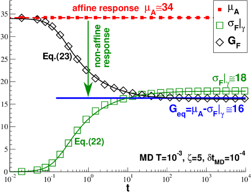
Figure 2: Affine shear elasticity $\mu_{\mathrm{A}}(t)$, shear stress fluctuations $\sigma_{\mathrm{F}}(t)|_{\gamma}$ and their difference $G_{\mathrm{F}}(t)=\mu_{\mathrm{A}}-\sigma_{\mathrm{F}}(t)|_{\gamma}$ as a function of the measurement time $t$ for one network of ideal springs in two dimensions ($\text{NV}\gamma\text{T}$-ensemble). The data have been sampled by MD simulation with time step $\delta t_{\mathrm{MD}}=10^{-4}$, temperature $T=10^{-3}$ and friction constant $\zeta=5$. The solid lines present a consistency check of $\sigma_{\mathrm{F}}(t)|_{\gamma}$ and $G_{\mathrm{F}}(t)$ with the correlation function $C(t)|_{\gamma}$ confirming Eq. (22) and Eq. (23).

Static properties at small finite temperatures.

We focus below on systems with a finite temperature $T=10^{-3}$. Since this temperature is rather small, one expects all static properties such as the pressure $P$ or the elastic modulus $G_{\mathrm{eq}}$ to be barely changed. As we have checked comparing various methods one confirms indeed that $P\approx P_{\mathrm{ex}}\approx 2$, $\mu_{\mathrm{A}}\approx 34$, $\sigma_{\mathrm{F}}|_{\gamma}\approx 18$ and $G_{\mathrm{eq}}\approx 16$ and the same applies to all small temperatures $T\ll 1$.

Convergence of stress-fluctuation formula.

How the shear modulus is obtained using the stress-fluctuating formula, Eq. (11), can be seen from Fig. 2 where we present data obtained by standard velocity-Verlet MD simulation Allen and Tildesley (1994); Frenkel and Smit (2002) using a (rather cautious) time step $\delta t_{\mathrm{MD}}=10^{-4}$. The temperature $T=10^{-3}$ is imposed by means of a Langevin thermostat with a large friction constant $\zeta=5$. We have used here one long production run over a time $t_{\mathrm{run}}=10^{5}$ for one equilibrated start configuration. Various properties, such as the instantaneous values of the shear stress $\hat{\tau}(t)$ or the affine shear elasticity $\hat{\mu}_{\mathrm{A}}(t)$, Eq. (10), have been written down at equidistant time steps $\delta t=10^{-2}$. The data correspond to averages taken first over a given time interval $[t_{0},t_{1}=t_{0}+t]$, i.e. using $1+t/\delta t$ entries, and taking then in a second step gliding averages over all times $t_{0}$ possible for $t$ Allen and Tildesley (1994). (Naturally, the error bars thus increase somewhat with $t$.) The horizontal axis in Fig. 2 indicates the interval length $t$. As one expects, the simple average $\mu_{\mathrm{A}}(t)$ becomes immediately constant (filled squares), i.e. $\mu_{\mathrm{A}}(t)=\mu_{\mathrm{A}}\approx 34$, as indicated by the dashed horizontal line foo (c). By contrast, the shear stress fluctuations $\sigma_{\mathrm{F}}(t)|_{\gamma}$ are seen to increase monotonously from zero to the asymptotic plateau $\sigma_{\mathrm{F}}|_{\gamma}\approx 18$. Interestingly, this plateau is only reached for surprisingly large times $t\gg 10^{3}$. The stress-fluctuation estimate $G_{\mathrm{F}}(t)\equiv\mu_{\mathrm{A}}-\sigma_{\mathrm{F}}(t)|_{\gamma}$ (diamonds) of the shear modulus $G_{\mathrm{eq}}$ decreases thus monotonously from $\mu_{\mathrm{A}}$ to its large-$t$ limit $G_{\mathrm{eq}}\approx 16$ indicated by the bold horizontal line. A too short production run thus leads to an overestimation of $G_{\mathrm{eq}}$. The two thin solid lines present a consistency check for $\sigma_{\mathrm{F}}(t)|_{\gamma}$ and $G_{\mathrm{F}}(t)$ integrating the shear stress autocorrelation function $C(t)|_{\gamma}$ as suggested by Eq. (22) and Eq. (23). The slow convergence of the stress-fluctuation relation $G_{\mathrm{F}}(t)$ noted in Refs. Schnell et al. (2011); Wittmer et al. (2013a) can thus be traced back to the sluggish $1/t$-decay of the second term in Eq. (23). We turn now to the description of $C(t)|_{\gamma}$ and other correlation functions.

IV.2 Computational test of key relation

Figure 3: Stress relaxation modulus $G(t)$ and stress autocorrelation functions $C(t)|_{\tau}$ (triangles) and $C(t)|_{\gamma}$ (squares) sampled by MD simulation. An affine strain $\gamma=10^{-2}$ is applied to determine $G(t)$. The filled triangles correspond to $C(t)|_{\tau}$ computed using one single trajectory with a slow MC shear-barostat with $\delta\gamma_{\mathrm{max}}=10^{-7}$, the crosses to a too large value $\delta\gamma_{\mathrm{max}}=10^{-5}$ for which $C(t)|_{\tau}$ is seen to decay rapidly due to additional relaxation pathways.

Introduction.

Having shown in Fig. 2 how a finite shear modulus $G_{\mathrm{eq}}\approx 16$ may be determined in the $\text{NV}\gamma\text{T}$-ensemble using the stress fluctuation formula, Eq. (11), we now demonstrate numerically our key relation, Eq. (4), by comparing the explicitly computed out-of-equilibrium stress relaxation modulus $G(t)$ with the equilibrium autocorrelation functions $C(t)|_{\gamma}$ and $C(t)|_{\tau}$. As before we show first in Fig. 3 data obtained by MD simulations using a high friction constant $\zeta=5$, which simplifies the data by enforcing a monotonic decay of the correlations. We discuss then results obtained using different friction constants and computational schemes.

Stress relaxation and autocorrelation functions.

The stress relaxation modulus $G(t)$ presented in Fig. 3 has been computed from the shear stress increment $\delta\hat{\tau}(t)$ measured after an affine shear strain $\gamma=10^{-2}$ was imposed at $t=0$ foo (b). We average over $10^{3}$ runs starting from independent reference configurations at $t=0^{-}$. The shear stress relaxation modulus $G(t)$ decreases (due to the strong damping) monotonously from $G(0^{+})=\mu_{\mathrm{A}}$ to a finite $G_{\mathrm{eq}}$. In contrast to this $C(t)|_{\gamma}$ (open squares) decays from $\sigma_{\mathrm{F}}|_{\gamma}$ to zero. Confirming Eq. (4), the vertically shifted autocorrelation function $C(t)|_{\gamma}+G_{\mathrm{eq}}$ (filled squares) is seen to collapse onto $G(t)$. The autocorrelation function $C(t)|_{\tau}$ (open triangles) has been obtained by preparing first an $\text{NV}\tau\text{T}$-ensemble of mean stress $\tau=0$ containing $10^{4}$ independent start configurations. We sample $\tilde{C}(t)|_{\gamma}$ and $\langle\hat{\tau}\rangle|_{\gamma}$ for each configuration keeping $\gamma$ constant and average then over all configurations, Eq. (12). Confirming Eq. (15) we observe $G(t)\approx C(t)|_{\tau}$.

Keeping the shear-barostat switched on.

As shown by the small filled triangles in Fig. 3, the same result is also obtained by sampling $\hat{\tau}(t)$ for every $\delta t=10^{-3}$ using an extremely slow shear-barostat for one single trajectory up to $t=10^{5}$. This large time is needed for a sufficient ensemble sampling. Otherwise, $\sigma_{\mathrm{F}}(t)|_{\tau}$ would remain below its asymptotic large-$t$ limit $\mu_{\mathrm{A}}=\sigma_{\mathrm{F}}|_{\tau}$ foo (c). We have used here a hyprid MD-MC scheme where after every MD step a Metropolis MC attempt was made to change the metric Wittmer et al. (2013a); foo (b) by a small amount $|\delta\gamma|\leq\delta\gamma_{\mathrm{max}}=10^{-7}$. Additional (non-universal) relaxation pathways become important if $\gamma(t)$ changes too strongly. If instead $\delta\gamma_{\mathrm{max}}=10^{-5}$ is used (all other parameters kept constant) this naturally leads to a rapid decay of $C(t)|_{\tau}$ (crosses). The conceptionally important point is here that in the limit of sufficiently small $\delta\gamma_{\mathrm{max}}$ Eq. (3) holds. The quenched $\text{NV}\tau\text{T}$-ensemble average $C(t)|_{\tau}$ (open triangles) is then obtained without completely switching off the shear-barostat. The detailed description of the presumably non-universal scaling of the additional relaxation pathways at larger $\delta\gamma_{\mathrm{max}}$ is of course also of interest. This should be addressed in future work.

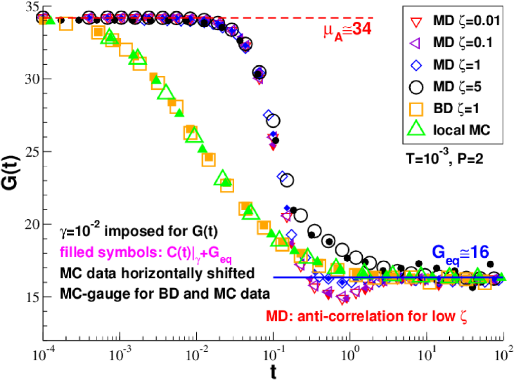
Figure 4: Stress relaxation modulus $G(t)$ (open symbols) and rescaled autocorrelation function $C(t)|_{\gamma}+G_{\mathrm{eq}}$ (filled symbols) for MD simulations for several friction constants $\zeta$, BD simulations with $\zeta=1$ and local MC moves. Shifting horizontally the MC data by a factor $1/8000$ allows to bring them to collapse onto the BD data.

Different numerical schemes.

The scaling collapse of $G(t)$ and $C(t)|_{\gamma}+G_{\mathrm{eq}}$ has been also obtained for different temperatures $T$ (not shown) and friction constants $\zeta$ as may be seen from Fig. 4. As one expects, the MD data decay more rapidly with decreasing $\zeta$ and reveal anti-correlations and oscillations for the lowest $\zeta$ probed. Also included in Fig. 4 is data obtained by (overdamped) BD simulations with a friction constant $\zeta=1$ and MC simulations with local monomer jump attempts uniformally distributed in a disk of radius $0.01$ Allen and Tildesley (1994). Both data sets for each simulation type are again found to collapse. Note that it is possible to collapse additionally the BD and MC data by shifting the MC data horizontally.

Gauge freedom for the instantaneous stress.

A technical point should finally be mentioned. While for our MD simulations the instantaneous shear stress $\hat{\tau}=\hat{\tau}_{\mathrm{id}}+\hat{\tau}_{\mathrm{ex}}$ comprises both an ideal contribution $\hat{\tau}_{\mathrm{id}}$ and an excess contribution $\hat{\tau}_{\mathrm{ex}}$ and correspondingly $\mu_{\mathrm{A}}=\mu_{\mathrm{A,id}}+\mu_{\mathrm{A,ex}}$ and $\sigma_{\mathrm{F}}|_{\gamma}=\sigma_{\mathrm{F,id}}|_{\gamma}+\sigma_{\mathrm{F,ex}}|_{\gamma}$ take ideal contributions $\mu_{\mathrm{A,id}}=\sigma_{\mathrm{F,id}}|_{\gamma}=P_{\mathrm{id}}$, this is not possible for BD and MC simulations. (Note that for the low temperature considered contributions of order $P_{\mathrm{id}}\approx 10^{-3}$ are in any case negligible.) Within the so-called “MC-gauge” Wittmer et al. (2013b), we thus set $\hat{\tau}_{\mathrm{id}}\equiv 0$ for BD and MC, i.e. the kinetic degrees of freedom are considered to be integrated out. Essentially we take advantage here of the general gauge freedom for the definition of instantaneous intensive variables foo (d). Note that for the demonstration of Eq. (4) we did not specify whether the state of the system is characterized by the positions and momenta of the particles (as in MD simulations) or only by their positions (as in BD and MC). To satisfy Eq. (4) it is just required that $\mu_{\mathrm{A}}$, $\sigma_{\mathrm{F}}|_{\gamma}$, $C(t)|_{\tau}$, $C(t)|_{\gamma}$ and $G(t)$ are measured consistently.

V Conclusion

Main results.

Focusing on permanent isotropic networks in thermal equilibrium (Sec. III) we have revisited theoretically (Sec. II.2) and numerically (Sec. IV.2) the linear-response relation between the shear stress relaxation modulus $G(t)$ and the shear stress autocorrelation functions $C(t)|_{\gamma}$ and $C(t)|_{\tau}$ computed, respectively, at imposed strain $\gamma$ and mean stress $\tau$. It has been demonstrated that according to Eq. (4) or Eq. (18) $G(t)=C(t)|_{\tau}$ and $C(t)|_{\gamma}$ must become different in the solid limit for $G_{\mathrm{eq}}>0$. While $G(t)$ may be determined numerically directly from $C(t)|_{\tau}$ using either a quenched $\text{NV}\tau\text{T}$-ensemble or an asymptotically slow shear-barostat for which Eq. (3) holds (Fig. 3), this is not possible alone from $C(t)|_{\gamma}$.

Digression.

More briefly, we have commented on self-assembled transient elastic networks characterized by a scission-recombination frequency $f$ for the springs (Sec. II.4). For a finite, but small frequency $f$ the shear modulus $G_{\mathrm{eq}}(f)$ must vanish for long sampling times. Following Ref. Sausset et al. (2010) we have argued that $G(t)=C(t)|_{\tau}=C(t)|_{\gamma}=G_{\mathrm{F}}(t)$ should reveal an intermediate plateau $G_{\mathrm{P}}$ and that this plateau is set by the finite shear modulus of the quenched network, $G_{\mathrm{P}}=G_{\mathrm{eq}}(f=0)$.

Discussion.

More generally, it is obviously often helpful to describe an observed intermediate plateau or shoulder of $G(t)$ in terms of a phenomenological shear modulus $G_{\mathrm{P}}$ of a dynamical model, such as the Maxwell model for viscoelastic fluids or the reptation model of entangled polymer melts Rubinstein and Colby (2003); Doi and Edwards (1986). However, such a model allowing the theoretical interpretation of the data should not be confused with the proper measurement procedure and the model parameter $G_{\mathrm{P}}$ should not be identified with the thermodynamic equilibrium modulus $G_{\mathrm{eq}}$ of the system. Note that the shear modulus $G_{\mathrm{eq}}$ of a Maxwell fluid or a linear polymer melt must vanish while the phenomenological parameter $G_{\mathrm{P}}$ describing the short or intermediate time stress response is finite. Since in this sense different operational “static” and “dynamical” definitions of the shear modulus are used for describing glass-forming liquids close to the glass transition Klix et al. (2012); Szamel and Flenner (2011); Yoshino (2012); Yoshino and Mézard (2010); Zaccone and Terentjev (2013), this may explain why qualitatively different temperature dependences (cusp singularity Yoshino and Mézard (2010); Zaccone and Terentjev (2013) vs. finite jump Götze (2009); Klix et al. (2012); Szamel and Flenner (2011); Ozawa et al. (2012)) have been predicted. Hence, while our recent attempts to determine $G_{\mathrm{eq}}(T)$ for two glass-forming model systems Wittmer et al. (2013a) are consistent with a continuous cusp, this is not necessarily in contradiction with a jump singularity for $G_{\mathrm{P}}(T)$ determined from $C(t)|_{\gamma}$ Klix et al. (2012); Ozawa et al. (2012).

Outlook.

It should be noted that generalizing Eq. (4) one obtains readily that

$$M(t)=C(t)|_{I}=C(t)|_{X}+M_{\mathrm{eq}}\ \mbox{ for }t>0$$ (29)

with $M(t)$ being the relaxation modulus of an intensive variable $I$, $M_{\mathrm{eq}}=\partial I/\partial X$ the associated equilibrium modulus and $C(t)=\beta V\langle\delta\hat{I}(t)\delta\hat{I}(0)\rangle$ the corresponding autocorrelation function for any (continuous) intensive variable $\hat{I}(t)$. We note finally that we are currently simulating transient elastic networks formed by dense, purely repulsive beads which are reversibly connected by harmonic springs. The preliminary results support Eq. (26) suggested in Sec. II.4, i.e. it is seen that $G(t)$, $C(t)|_{\gamma}$ and $G_{\mathrm{F}}(t)$ approach with decreasing, but finite scission-recombination frequency $f$, i.e. $G_{\mathrm{eq}}(f)=0$, an intermediate plateau given by the shear modulus $G_{\mathrm{eq}}(f=0)$ of the quenched reference network foo (g).