Numerical solution for the Schwinger–Dyson equation
at finite temperature in Abelian gauge theory

Abstract

We present the exact numerical solutions for the Schwinger–Dyson equations at finite temperature with general gauge in Abelian gauge theory. We then study the chiral phase transition on temperature from the obtained solutions. We find that, within the quenched Schwinger–Dyson equations, there exists substantial gauge dependence on the solutions and the critical temperature.

I Introduction

The chiral phase transition at finite temperature is an important and interesting phenomenon in gauge theories. The chiral symmetry is broken for low temperature in the strongly coupling system, and expected to be restored for high temperature. Then, it is interesting to investigate this critical behavior; in particular, the critical temperature on the chiral phase transition.

The Schwinger–Dyson equation (SDE) Dyson:1949ha is frequently used method for the studies on the above mentioned chiral phase transition. The SDE are the integral equations for the green functions, and the solutions lead the field strength renormalization and the dynamically generated mass (for reviews, see, Roberts:1994dr ; Roberts:2000aa ; Holl:2006ni ). A lot of works have been devoted to the analyses on the SDE at zero temperature Johnson:1964da ; Maskawa:1974vs ; FK76 ; Ball:1980ay ; Roberts:1989mj ; Curtis:1990zs ; Bando:1993qy ; Kizilersu:2009kg ; Kizilersu:2014ela and finite temperature Ikeda:2001vc ; Akiba:1987dr ; Kalashnikov:1987td ; Harada:1998zq ; Fukazawa:1999aj ; Fueki:2002mm ; Mueller:2010ah ; Nakkagawa:2011ci . The investigations at finite temperature are rather limited comparing to the ones at zero temperature, since it becomes difficult to solve the equations at finite temperature due to the separation of the time and space components LeBellac . Then the preceding works have mostly been done through employing some approximations on the equations in a specific gauge. However, it is possible to evaluate the equations without approximations Ikeda:2001vc . In this paper, we shall solve the SDE at finite temperature without approximations in general gauge. Thereafter we study the gauge dependence on the chiral phase transition with respect to temperature.

The plan of the paper is as follows. Section II presents the equations at finite temperature and the prescription of solving the equations. The numerical solutions and the critical behavior are shown in Secs. III and IV. The concluding remarks are given in Sec. V.

II Schwinger–Dyson equation

We will here present the SDE at finite temperature and the iteration method which is the numerical procedure employed in this letter.

II.1 The equations at finite temperature

The equation for the fermion self-energy $\Sigma(p)$ is given by

$$\Sigma(p)=ie^{2}\int\frac{{\mathrm{d}}^{4}q}{(2\pi)^{4}}\gamma^{\mu}D_{\mu\nu}(p-q)S(q)\Gamma^{\nu}(p,q),$$ (1)

with the coupling strength, $e$, the propagators for the photon and fermion, $D_{\mu\nu}(p-q)$ and $S(q)$, and the vertex function $\Gamma^{\nu}(p,q)$. For $D_{\mu\nu}$ and $\Gamma^{\nu}$, we use the following quenched forms

$$D_{\mu\nu}(k)=\frac{-g_{\mu\nu}}{k^{2}}+(1-\xi)\frac{k_{\mu}k_{\nu}}{k^{4}},$$ (2)

$$\Gamma^{\nu}(p,q)=\gamma^{\nu},$$ (3)

where $\xi$ is the gauge parameter and $k_{\mu}=p_{\mu}-q_{\mu}$.

The fermion propagator is defined by

$$S(p_{0},p)=\frac{1}{C(p_{0},p)\gamma_{0}p_{0}+A(p_{0},p)\gamma_{i}p^{i}-B(p_{0},p)}$$ (4)

with $p=|{\bf p}|$. Note that the time and space components are to be treated separately for the extension to finite temperature. In the imaginary time formalism, the continuous $q_{0}$ integral is replaced by the discretized summation due to the applied boundary condition LeBellac ,

$$\frac{1}{2\pi i}\int_{-\infty}^{\infty}\mathrm{d}q_{0}F(q_{0})\to T\sum_{m=-\infty}^{\infty}F(i\omega_{m})$$ (5)

where $T$ is the temperature of the system. The frequency, $\omega_{m}$, is taken as

$$\omega_{m}=(2m+1)\pi T$$ (6)

for the fermionic field.

After some algebras one obtains the following equations

$$C(\omega_{n},p)=1+\frac{\alpha}{\pi}T\sum_{m=-\infty}^{\infty}\int_{\lambda}^{\Lambda}\mathrm{d}q\,\left[{\mathcal{I}}_{CC}C(\omega_{m},q)+{\mathcal{I}}_{CA}A(\omega_{m},q)\right]\Delta(\omega_{m},q),$$ (7)

$$A(\omega_{n},p)=1+\frac{\alpha}{\pi}T\sum_{m=-\infty}^{\infty}\int_{\lambda}^{\Lambda}\mathrm{d}q\,\left[{\mathcal{I}}_{AC}C(\omega_{m},q)+{\mathcal{I}}_{AA}A(\omega_{m},q)\right]\Delta(\omega_{m},q),$$ (8)

$$B(\omega_{n},p)=m_{0}+\frac{\alpha}{\pi}T\sum_{m=-\infty}^{\infty}\int_{\lambda}^{\Lambda}\mathrm{d}q\,\left[{\mathcal{I}}_{B}B(\omega_{m},q)\right]\Delta(\omega_{m},q),$$ (9)

with $\alpha=e^{2}/(4\pi)$,

$$\Delta(\omega_{m},q)=\frac{1}{C^{2}(\omega_{m},q)\omega_{m}^{2}+A^{2}(\omega_{m},q)q^{2}+B^{2}(\omega_{m},q)}.$$ (10)

and

$${\mathcal{I}}_{CC}=-\xi_{+}\frac{{\omega_{m}}}{\omega_{n}}I_{1}+2\xi_{-}\frac{{\omega_{m}}}{\omega_{n}}{\omega^{\prime}_{m}}^{2}I_{2},$$ (11)

$${\mathcal{I}}_{CA}=\xi_{-}\frac{\omega^{\prime}_{m}}{\omega_{n}}I_{1}+\xi_{-}\frac{\omega^{\prime}_{m}}{\omega_{n}}\left[{\omega^{\prime}_{m}}^{2}-q^{2}+p^{2}\right]I_{2},$$ (12)

$${\mathcal{I}}_{AC}=-\xi_{-}\frac{{\omega_{m}}{\omega^{\prime}_{m}}}{p^{2}}I_{1}-\xi_{-}\frac{{\omega_{m}}{\omega^{\prime}_{m}}}{p^{2}}\left[{\omega^{\prime}_{m}}^{2}+q^{2}-p^{2}\right]I_{2},$$ (13)

$${\mathcal{I}}_{AA}=-\frac{2q^{2}}{p^{2}}-\frac{1}{2p^{2}}\left[\xi_{3}^{-}{\omega^{\prime}_{m}}^{2}+\xi_{+}(q^{2}+p^{2})\right]I_{1}-\frac{1}{2p^{2}}\xi_{-}\left[{\omega^{\prime}_{m}}^{4}-(q^{2}-p^{2})^{2}\right]I_{2},$$ (14)

$${\mathcal{I}}_{B}=-\xi_{3}^{+}I_{1},$$ (15)

$$I_{1}=\frac{q}{2p}\ln\frac{{\omega^{\prime}_{m}}^{2}+(q-p)^{2}}{{\omega^{\prime}_{m}}^{2}+(q+p)^{2}},$$ (16)

$$I_{2}=\frac{q}{2p}\left[\frac{1}{{\omega^{\prime}_{m}}^{2}+(q-p)^{2}}-\frac{1}{{\omega^{\prime}_{m}}^{2}+(q+p)^{2}}\right].$$ (17)

Here ${\omega^{\prime}_{m}}\equiv{\omega_{n}}-{\omega_{m}}$, $\xi_{\pm}\equiv 1\pm\xi$ and $\xi_{3}^{\pm}=3\pm\xi$, and we introduced the infrared and ultraviolet cutoffs, $\lambda$ and $\Lambda$. These equations are the set of the Schwinger–Dyson equations at finite temperature which are the straightforward extension from the equations at zero temperature with three dimensional momentum cutoff Kohyama:2015fta .

Once the solutions are obtained, we can evaluate the dynamical mass and the chiral condensate through the relations,

$$M(\omega_{n},p)=B(\omega_{n},p)/A(\omega_{n},p),$$ (18)

$$\phi=\langle\bar{\psi}\psi\rangle=-T\sum_{m=-\infty}^{\infty}\int\frac{\mathrm{d}^{3}q}{(2\pi)^{3}}{\rm tr}\left[\frac{B(\omega_{m},q)}{C^{2}(\omega_{m},q)\omega_{m}^{2}+A^{2}(\omega_{m},q)q^{2}+B^{2}(\omega_{m},q)}\right].$$ (19)

It should be noted that the chiral condensate becomes zero when the dynamical mass vanishes. Therefore one can see whether the chiral symmetry is broken, $\phi\neq 0$, from the value of $M(\omega_{n},p)$. Strictly, the phase transition should be evaluated at the minimum of the effective potential which is derived by integrating out the gap equation with respect to the order parameter. However, it is known to be adequate to see the solution of the gap equation in the system at zero chemical potential Harada:1998zq , then we search the critical temperature on the chiral phase transition by checking the value of the dynamical mass in this paper.

II.2 The iteration method

In this subsection, we discuss the numerical procedure for the integral equations. To briefly present the basic idea of the iteration method, we show the equations with the trapezoidal rule. (In the actual calculations, we used the Gauss-Legendre integration for the $q-$integration.)

In solving the equations, we discretize the integral to discrete summation as

$$C_{nj}^{(l)}=1+\frac{\alpha}{\pi}T\sum_{m=-N_{t}}^{N_{t}-1}\delta\sum_{k=0}^{N_{p}-1}\left[{\mathcal{I}}^{CC}_{njmk}C_{mk}^{(l-1)}+{\mathcal{I}}^{CA}_{njmk}A_{mk}^{(l-1)}\right]\Delta_{mk}^{(l-1)},$$ (20)

$$A_{nj}^{(l)}=1+\frac{\alpha}{\pi}T\sum_{m=-N_{t}}^{N_{t}-1}\delta\sum_{k=0}^{N_{p}-1}\left[{\mathcal{I}}^{AC}_{njmk}C_{mk}^{(l-1)}+{\mathcal{I}}^{AA}_{njmk}A_{mk}^{(l-1)}\right]\Delta_{mk}^{(l-1)},$$ (21)

$$B_{nj}^{(l)}=m_{0}+\frac{\alpha}{\pi}T\sum_{m=-N_{t}}^{N_{t}-1}\delta\sum_{k=0}^{N_{p}-1}\left[{\mathcal{I}}^{B}_{njmk}B_{mk}^{(l-1)}\right]\Delta_{mk}^{(l-1)},$$ (22)

with $\delta\equiv(\Lambda-\lambda)/N_{p}$. Note that we introduce the cutoff on the frequency summation since it is technically impossible to take the infinite number of summation. However, as will be confirmed by the numerical calculations in the next section, the contributions from the large number of $n$ and $m$ are negligible, then the artifact of setting $N_{t}$ does not affect the solutions if we choose large enough number for $N_{t}$. The matrix of the form $F_{njmk}$ indicates

$$F_{njmk}=F(\omega_{n},p,\omega_{m},q),\quad p=\lambda+\delta j,\quad q=\lambda+\delta k,$$ (23)

and the superscript $l$ in $F^{(l)}$ means the number of iteration. Therefore, the $l\,$th solutions, $F^{(l)}$, are derived from the equations with the previous solutions, $F^{(l-1)}$. By setting the initial conditions on $C^{(0)}$, $A^{(0)}$ and $B^{(0)}$ then carrying out the enough times of iterations, one can obtain the solutions.

III Numerical solution

Having presented the equations and the procedure of solving them, we are now ready to perform the numerical analyses. In this section, we are going to show the numerical solutions for $C$, $A$ and $B$ with respect to $\omega_{n}$, $p$, and temperature.

III.1 Solutions for $C(\omega_{n},p)$, $A(\omega_{n},p)$, $B(\omega_{n},p)$

Figure 1 displays the solutions of $C(\omega_{n},p)$, $A(\omega_{n},p)$, $B(\omega_{n},p)$ for $\alpha=3.5$, $\lambda=0.01\Lambda$, $m_{0}=0$ with $\xi=3$, $1$ and $0$ at temperatures $T=0.05\Lambda$ and $0.15\Lambda$. In carrying out the calculations, we took the number of frequency summation $N_{t}=50$ and performed the $100$ times of iterations. We have numerically confirmed that these numbers are good enough in our present analyses, namely the solutions well converge with $N_{t}=50$ and $N_{i}=100$. Then, we will persistently use this setting in what follows.

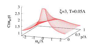
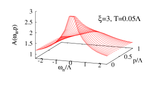
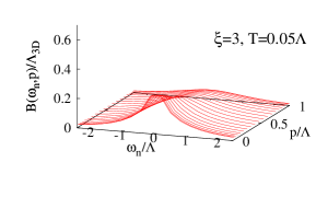
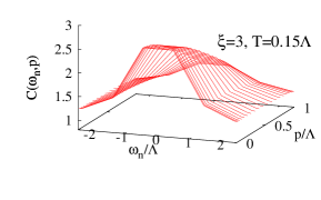
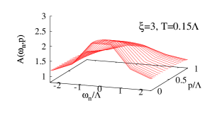
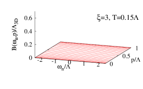
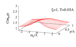
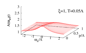
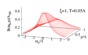
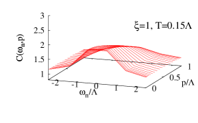
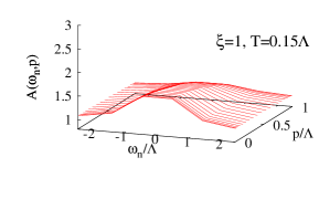
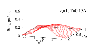
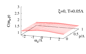
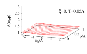
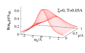
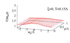
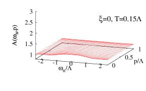
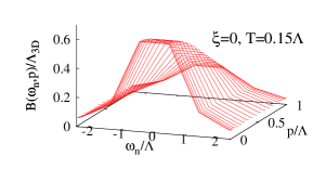
Figure 1: $C(\omega_{n},p)$, $A(\omega_{n},p)$, $B(\omega_{n},p)$ with $\alpha=3.5$, for $T=0.05\Lambda$ and $T=0.15\Lambda$.

From Fig. 1, one sees that $C$, $A$ and $B$ decrease with increasing temperature, and these shapes become smoother when temperature increases. This result on temperature can be understood easily, since the non-perturbative effect is expected to be suppressed at high temperature. Therefore the symmetry tends to be restored at high temperature, which can be confirmed by the obtained solutions. On the gauge dependence, the values of $C$ and $A$ are large for large $\xi$, while $B$ becomes smaller with respect to $\xi$. It is known from the $T=0$ analyses with the four dimensional momentum cutoff regularization that $C(=A)$ and $A$ become $1$ in the Landau gauge $\xi=0$. Then the deviation from $1$ is expected to become larger when $\xi$ increases, which is confirmed by the obtained results. On the other hand, the value of $B$ is small for large $\xi$. This comes from the fact that the denominator of the fermion propagator becomes larger when $C$ and $A$ raise up, then the integral in the equation for $B$ becomes small, leading smaller value for $B$ consequently.

III.2 Temperature dependence on the solutions

For the purpose to see the temperature dependence, it may be nice to display the figures with the temperature axis.

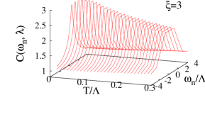
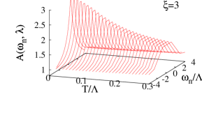
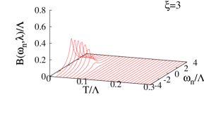
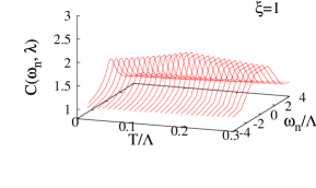
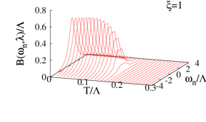
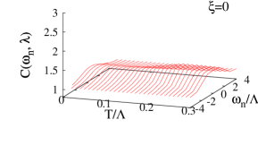
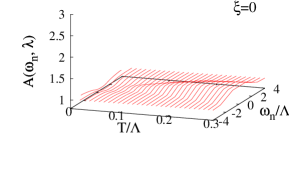
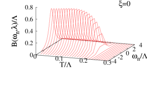
Figure 2: $C(\omega_{n},\lambda)$, $A(\omega_{n},\lambda)$, $B(\omega_{n},\lambda)$ for $\alpha=3.5$.

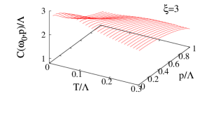
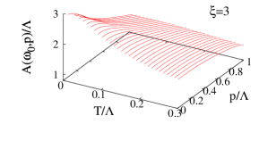
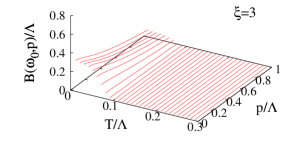
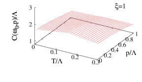
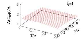
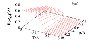
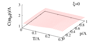
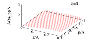
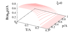
Figure 3: $C(\omega_{0},p)$, $A(\omega_{0},p)$, $B(\omega_{0},p)$ for $\alpha=3.5$.

Figures 2 and 3 show the temperature dependence on $C(\omega_{n},\lambda)$, $A(\omega_{n},\lambda)$, $B(\omega_{n},\lambda)$, and $C(\omega_{0},p)$, $A(\omega_{0},p)$, $B(\omega_{0},p)$. We observe that $C$ and $A$ slightly increases according to $T$ when $B\neq 0$, then decreases after $B$ vanishes. While the result of $B$ is easier to see; it stays almost constant for low $T$, then drops at certain $T$. This is the clear signal of the phase transition, where the mass factor $B$ becomes zero at some critical temperature $T_{c}$. The issue is interesting; we will discuss on this in more detail in the next section.

IV Chiral phase transition

We have shown rough shapes of the solutions by aligning the three dimensional figures in the previous section. We will now discuss the gauge dependence on the chiral phase transition in more detail focusing on the solutions at the lowest frequency and momentum, i.e., the values at $(\omega_{n},p)=(\omega_{0},\lambda)$.

IV.1 Gauge dependence on the solutions

Figure 4 shows how the solutions $C(\omega_{0},\lambda)$, $A(\omega_{0},\lambda)$, $B(\omega_{0},\lambda)$ and $M(\omega_{0},\lambda)$ changes with respect to $T$.

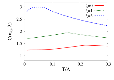
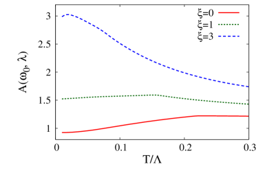
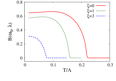
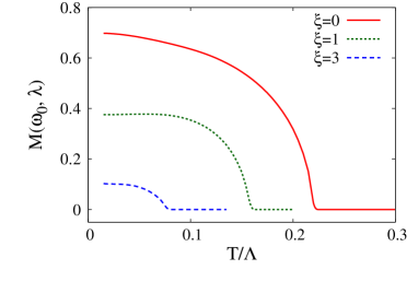
Figure 4: $C$, $A$, $B$ and $M$ as the functions of $T$ with $\alpha=3.5$ for $\xi=0$, $1$ and $3$ .

As we previously saw that $C$ increases with $T$ when $B$ is nonzero, then decreases after $B$ vanishes. $A$ shows the similar curves for $\xi=0$ and $1$, while it almost monotonously decreases for $\xi=3$. $B$ and $M$ become small for high $T$ as already observed in Figs. 2 and 3.

From the figure, one can clearly confirm the quantitative gauge dependence on the solutions. $C$ and $A$ are around $3$ for low $T$ with $\xi=3$, and within the range of around $1-2$ for $\xi=0$ and $1$. $M$ at $T=0$ is around $0.7$ for $\xi=0$ and it becomes considerably smaller for $\xi=3$. Thus, there exists the indispensable gauge dependence on the solutions for the quenched SDE.

IV.2 Critical temperature

Let us study the critical temperature, $T_{c}$, of the chiral phase transition here. We have discussed that the dynamically generated mass can be regarded as the order parameter of the transition in Sec. II.1. Then we shall carefully search the critical temperature of the chiral phase transition by evaluating the value of $M$.

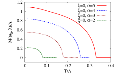
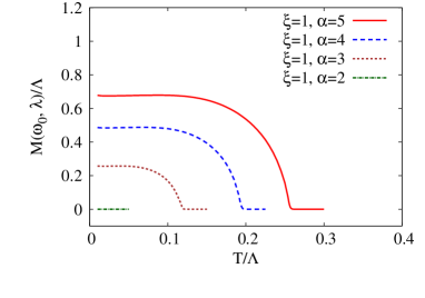
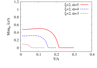
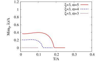
Figure 5: $M(\omega_{0},\lambda)$ as the functions of $T$ for various $\xi$ and $\alpha$.

Figure 5 displays the temperature dependence on the dynamical mass, $M(\omega_{0},\lambda)$, for various $\xi$ and $\alpha$. The critical temperature becomes larger when $\alpha$ increases. This can be easily understood since the system has stronger correlation for larger coupling. While $T_{c}$ is smaller for larger $\xi$. This comes from the effect of the field renormalization as we have seen from the preceding section. The explicit numbers of the critical temperature for various $\xi$ and $\alpha$ are aligned in Tab. 1.

Table 1: Critical temperature ($T_{c}/\Lambda$).

	$\alpha=2$	$\alpha=3$	$\alpha=4$	$\alpha=5$
$\xi=0$	$0.089$	$0.187$	$0.267$	$0.341$
$\xi=1$	—	$0.126$	$0.203$	$0.265$
$\xi=2$	—	$0.07$	$0.162$	$0.223$
$\xi=3$	—	—	$0.14$	$0.197$

Finally, we show $T_{c}$ as the function of $\alpha$ in Fig. 6.

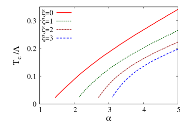
Figure 6: Critical temperature with respect to $\alpha$.

We again confirm that there exists substantial gauge dependence on the critical behavior. Note that we can not extend the curves for very low temperature within this formalism, since we need to take large number of frequency summation to get reliable results for low $T_{c}$ Chen:2009mv , which requires enormous calculation time. However one easily sees the limiting values on the critical coupling for $T_{c}\to 0$ from the figure, which are around $\alpha_{c}\simeq 1.2$, $2$, $2.6$ and $3$ for $\xi=0$, $1$, $2$ and $3$. It may be interesting to mention that these values are close to the ones obtained in the SDE with the four dimensional cutoff regularization at $T=0$, which leads $\alpha_{c}\simeq\pi/3$, $2$ and $3$ for $\xi=0$, $1$ and $3$ Kizilersu:2014ela .

V Concluding remarks

We have evaluated the numerical solutions for the SDE at finite temperature without approximations in Abelian gauge theory in this paper. There we observe the considerable gauge dependence on the solutions. We also analyzed the critical behavior of the chiral phase transition within the SDE approach. We confirm that the critical temperature as well drastically depends on the chosen gauge. This indicates that, when one investigates the chiral phase transition in the quenched SDE with using some approximations, one should be very careful on the set of assumptions. In particular, the field renormalization factors $C$ and $A$ nonnegligibly deviate from the unity for nonzero $\xi$.

Since we started from the SDE with the quenched form, then the gauge dependence as observed in this analysis is inevitable. This is clearly unsatisfactory feature of the quenched equations. Therefore the further analyses with generalized equations, such as the unquenched investigations Kizilersu:2014ela , or the extended vertex Ball:1980ay ; Curtis:1990zs ; Kizilersu:2009kg and coupling Roberts:1989mj , are obviously needed; this should be the future direction in the analyses based on the Schwinger–Dyson equation.

- (1) F. J. Dyson, Phys. Rev. 75, 1736 (1949). J. S. Schwinger, Proc. Nat. Acad. Sci. 37, 452 (1951).
- (2) C. D. Roberts and A. G. Williams, Prog. Part. Nucl. Phys. 33, 477 (1994).
- (3) C. D. Roberts and S. M. Schmidt, Prog. Part. Nucl. Phys. 45, S1 (2000).
- (4) A. Holl, C. D. Roberts and S. V. Wright, nucl-th/0601071.
- (5) K. Johnson, M. Baker and R. Willey, Phys. Rev. 136, B1111 (1964).
- (6) T. Maskawa and H. Nakajima, Prog. Theor. Phys. 52, 1326 (1974); ibid. 54, 860 (1975).
- (7) R. Fukuda and T. Kugo, Nucl. Phys. B 117, 250 (1976).
- (8) J. S. Ball and T. W. Chiu, Phys. Rev. D 22, 2542 (1980).
- (9) C. D. Roberts and B. H. J. McKellar, Phys. Rev. D 41, 672 (1990).
- (10) D. C. Curtis and M. R. Pennington, Phys. Rev. D 42, 4165 (1990).
- (11) M. Bando, M. Harada and T. Kugo, Prog. Theor. Phys. 91, 927 (1994).
- (12) A. Kizilersü and M. R. Pennington, Phys. Rev. D 79, 125020 (2009).
- (13) A. Kizilersü, T. Sizer, M. R. Pennington, A. G. Williams and R. Williams, Phys. Rev. D 91, no. 6, 065015 (2015); and references therein.
- (14) T. Ikeda, Prog. Theor. Phys. 107, 403 (2002).
- (15) T. Akiba, Phys. Rev. D 36, 1905 (1987).
- (16) O. K. Kalashnikov, Z. Phys. C 39, 427 (1988).
- (17) M. Harada and A. Shibata, Phys. Rev. D 59, 014010 (1999).
- (18) K. Fukazawa, T. Inagaki, S. Mukaigawa and T. Muta, Prog. Theor. Phys. 105, 979 (2001).
- (19) Y. Fueki, H. Nakkagawa, H. Yokota and K. Yoshida, Prog. Theor. Phys. 110, 777 (2003).
- (20) J. A. Mueller, C. S. Fischer and D. Nickel, Eur. Phys. J. C 70, 1037 (2010).
- (21) H. Nakkagawa, H. Yokota and K. Yoshida, Phys. Rev. D 85, 031902 (2012); ibid. 86, 096007 (2012).
- (22) M. L. Bellac, Thermal Field Theory (Cambridge University Press, 1996).
- (23) H. Kohyama, arXiv:1507.08231 [hep-ph].
- (24) J. W. Chen, K. Fukushima, H. Kohyama, K. Ohnishi and U. Raha, Phys. Rev. D 81, 071501 (2010).