On the construction of virtual interior point source travel time distances from the hyperbolic Neumann-to-Dirichlet map

Abstract

We introduce a new algorithm to construct travel time distances between a point in the interior of a Riemannian manifold and points on the boundary of the manifold, and describe a numerical implementation of the algorithm. It is known that the travel time distances for all interior points determine the Riemannian manifold in a stable manner. We do not assume that there are sources or receivers in the interior, and use the hyperbolic Neumann-to-Dirichlet map, or its restriction, as our data. Our algorithm is a variant of the Boundary Control method, and to our knowledge, this is the first numerical implementation of the method in a geometric setting.

1 Introduction

We consider the inverse boundary value problem for the acoustic wave equation on a domain or on a Riemannian manifold $M$. The problem is to recover a spatially varying sound speed $c$ inside the domain given the corresponding Neumann-to-Dirichlet map, or its restriction on a part of the boundary of the domain, say $\Gamma\subset\partial M$.

In the acoustic case, waves propagate in a domain $M$ with speed $c$, and the travel time of a wave between a pair of points $x$ and $y$ in $M$ is given by the Riemannian distance $d(x,y)$ when computed with respect to the travel time metric $c^{-2}dx^{2}$. For this reason, it is natural to formulate the inverse boundary value problem by using concepts from Riemannian geometry. This also allows us to consider anisotropic sound speeds in a unified way.

We present a new method to use the local restriction of the Neumann-to-Dirichlet map to determine travel time distances of the form $d(x,y)$ where $x$ is a point in the interior of the domain and $y\in\Gamma$, that is, $y$ is a point in the set where we have boundary measurements. We refer to these travel times as point source travel time data, since the distance $d(x,y)$ corresponds to the first arrival travel time from a (virtual) interior point source located at $x$ as recorded at the boundary at $y$. We emphasize that our method synthesizes the travel times from a point source in the interior of $M$ without requiring an actual receiver or source at that location.

Using the travel time distances we can introduce Dirac boundary sources which generate waves the singularities of which focus in a point. Such boundary sources have been referred to as focusing functions in reflection seismology [37].

To motivate our results, we note that travel times have previously been shown to determine a Riemannian manifold with boundary see e.g. [19]. In particular, in the full boundary data case, it has been shown that this determination is even stable [20]. Furthermore, it can be shown that travel times determine shape operators that appear as data for the generalized Dix method [14]. This is of particular interest in the isotropic case, since that method allows for the local nonlinear reconstruction of a sound-speed near geodesic rays.

Our method to determine boundary distances works by first using a variant of the Boundary Control method (BC method) to determine volumes of subdomains of $M$ referred to as wave caps. The volumes are computed by solving a collection of regularized ill-posed linear problems. The BC method originates from [6], where it was used to solve the inverse boundary problem for the acoustic wave equation. We note that [8] was the first variant of the BC method posed in a geometric setting. For a thorough overview of the BC method, we refer to [19] and [7]. Regularization theory was first combined with the BC method in [10], and the procedure that we use to determine volumes was developed in [28].

In the present paper, we introduce a procedure to construct point source travel time data from the volumes of wave caps, and hence reduce the inverse boundary value problem to the stable problem of determining the Riemannian manifold $(M,g)$ given the point source travel time data. In particular, our procedure splits the inverse boundary value problem to an ill-posed but linear step (the volume computation) and a non-linear but well-posed step (distance estimation and reconstruction of the manifolds).

We describe a computational implementation of our method, and provide a numerical example to demonstrate our technique. We remark that our numerical example provides the first computational realization of a geometric variant of the BC method. Moreover, we explain how the instability of the volume computation step is manifest in our numerical examples. All variants of the BC method that use partial data contain similar unstable steps, and we believe that the instability of the method reflects the ill-posedness of the inverse boundary value problem itself. However, contrary to Calderón’s problem, that is, the elliptic inverse boundary value problem [12, 34], it is an open question whether the inverse boundary value problem for the wave equation is ill-posed in general. For results concerning the stability of Calderón’s problem we refer to [1, 26].

Also, we point out that under favorable geometric assumptions, the hyperbolic inverse boundary value problem is known to have better stability properties than Calderón’s problem, see e.g. [9, 24, 27, 32, 33] and references therein. However, these geometric assumptions do not apply to the partial data problem that we consider here.

2 Statement of the Results

In this section we describe our data and assumptions, and what we intend to recover from the data.

2.1 Direct problem as a model for measurements

We work in the following setting,

Assumption 1.

$M$ is a smooth compact connected manifold with smooth boundary $\partial M$, and $g$ is an unknown smooth Riemannian metric on $M$.

Let $\mu\in C^{\infty}(\overline{M})$ be a strictly positive weight function, note that we do not require any additional information about $\mu$. We consider the following wave equation on $(M,g)$ with boundary source $f\in C_{0}^{\infty}((0,\infty)\times\partial M)$,

(1) $$\begin{array}[]{lr}\partial_{t}^{2}u(t,x)-\Delta_{g,\mu}u(t,x)=0,&(t,x)\in(0,\infty)\times M,\\ N_{\mu}u(t,x)=f(t,x),&(t,x)\in(0,\infty)\times\Gamma\\ u(0,\cdot)=0,\quad\partial_{t}u(0,\cdot)=0,&x\in M.\end{array}$$

The operator $\Delta_{g,\mu}$ is the weighted Laplace-Beltrami operator, given by,

$$\Delta_{g,\mu}w(x):=\mu^{-1}\operatorname{div_{g}}(\mu\operatorname{grad_{g}}(w)),$$

and, $N_{\mu}$ is the associated Neumann derivative,

$$N_{\mu}w:=-\mu\left\langle\nu,\operatorname{grad_{g}}(w)\right\rangle_{g},$$

where $\nu$ is the inward pointing unit normal vector to $\partial M$ in the metric $g$, $\operatorname{div_{g}}$ and $\operatorname{grad_{g}}$ are respectively the divergence and gradient on $(M,g)$, and $\langle\cdot,\cdot\rangle_{g}$ denotes the inner product with respect to the metric $g$. We remark that $\Delta_{g,\mu}$ is defined so that we can also handle the usual acoustic wave equation. Indeed, if we consider a domain $M\subset\mathbb{R}^{n}$ along with a strictly positive function $c\in C^{\infty}(\overline{M})$, then with respect to the conformally Euclidean metric $g=c^{-2}dx^{2}$, the weight $\mu=c^{n-2}$ yields $\Delta_{g,\mu}=c^{2}\Delta$.

We now introduce our data model. We denote the solution to (1) with Neumann boundary source $f$ by $u^{f}(t,x)$. For $T>0$, and $\Gamma\subset\partial M$ an open set, we define the local Neumann-to-Dirichlet operator associated with (1) by,

$$\Lambda_{\Gamma}^{2T}:f\mapsto u^{f}|_{(0,2T)\times\Gamma},\quad f\in C_{0}^{\infty}((0,2T)\times\Gamma).$$

The map $\Lambda_{\Gamma}^{2T}$ extends to a bounded operator on $L^{2}((0,2T)\times\Gamma)$, see for instance [22]. For data, we suppose that $\Lambda_{\Gamma}^{2T}$ is known. We note that $\Lambda_{\Gamma}^{2T}$ models boundary measurements for waves generated with acoustic sources and receivers located on $\Gamma$, where the waves are both generated and recorded on $\Gamma$ for $2T$ units of time. In addition, we note that in seismic applications the Neumman-to-Dirichlet map appears in simultaneous source acquisition.

Our primary interest is in constructing distances with respect to the Riemannian metric $g$, and we denote the Riemannian distance between the points $x,y\in M$ by $d(x,y)$. To simplify our distance computation procedure, we assume:

Assumption 2.

The distances $d(y,z)$ are known for $y,z\in\Gamma$ with $d(y,z)<T$.

We note that this is not a major limitation since for $y,z\in\Gamma$ with $d(y,z)<T$, the data $\Lambda_{\Gamma}^{2T}$ determines $d(y,z)$, see e.g. [13, Section 2.2].

2.2 Reconstruction of the point source travel time data

We define $R(M)$ to be the set of boundary distance functions on $M$,

(2) $$R(M)=\{r_{x}:x\in M,\text{ and for $z\in\partial M$, $r_{x}(z):=d(x,z)$}\}.$$

We note that, for $x\in M$ and $z\in\partial M$, $r_{x}(z)$ gives the minimum travel time from $x$ to $z$. With this interpretation, $r_{x}(z)$ represents the first arrival time at $z$ from a wave generated by a point source located at $x$.

In Section 3 we develop a method to synthesize values of $r_{x}$ from $\Lambda_{\Gamma}^{2T}$ for points $x$ indexed by a set of coordinates known as semi-geodesic coordinates. We refer to this procedure as forming point source travel time data, since our procedure reproduces the travel time information for a point source located at $x$ without having a source or receiver there.

The geometry of the supports of solutions to (1) inform our constructions. To be explicit, let $\tau$ be a function on $\Gamma$ satisfying $0\leq\tau(z)\leq T$ for all $z\in\Gamma$ and define the domain of influence of $\tau$,

$$M(\tau):=\left\{x\in M\ :\ \text{there exists a $z\in\bar{\Gamma}$ such that $d(x,z)\leq\tau(z)$}\right\}.$$

We depict $M(\tau)$ in Figure 1a. Consider the set

(3) $$S_{\tau}:=\{(t,z)\in(0,T)\times\bar{\Gamma}:\ t\in(T-\tau(z),T)\}.$$

We recall that solutions to (1) exhibit finite speed of propagation in the metric $g$, and specifically, if $\mathop{\operator@font supp}\nolimits(f)\subset S_{\tau}$ then $\mathop{\operator@font supp}\nolimits(u^{f}(T,\cdot))\subset M(\tau)$.

When $\tau$ is a multiple of an indicator function, we will occasionally use a special notation for $M(\tau)$. To be specific, we denote the indicator function of a set $S$ by $1_{S}$, and for $s\geq 0$ we will use the notation $M(\Gamma,s):=M(s1_{\Gamma})$ and $M(y,s):=M(s1_{\{y\}})$.

We denote the unit sphere bundle $SM:=\{\xi\in TM:\ |\xi|_{g}=1\}$, and define the inward/outward pointing sphere bundles by $\partial_{\pm}SM:=\{\xi\in\partial SM:\ (\xi,\pm\nu)_{g}>0\}$, where $\nu$ is the inner unit normal vector field on $\partial M$. We define the exit time for $(x,\xi)\in SM\setminus\overline{\partial_{+}SM}$, by

$$\tau_{M}(x,\xi):=\inf\{s\in(0,\infty):\ \gamma(s;x,\xi)\in\partial M\},$$

where $\gamma(\cdot;x,\xi)$ is the geodesic with the initial data $\gamma(0)=x$, $\dot{\gamma}(0)=\xi$.

For $y\in\Gamma$ we define $\sigma_{\Gamma}(y)$ to be the maximal arc length for which the normal geodesic beginning at $y$ minimizes the distance to $\Gamma$. That is,

$$\sigma_{\Gamma}(y) :=\max\{s\in(0,\tau_{M}(y,\nu)]:\ d(\gamma(s;y,\nu),\Gamma)=s\}.$$

We recall, see e.g. [19, p. 50] that $\sigma_{\Gamma}(y)>0$ for $y\in\Gamma$. Moreover, $\sigma_{\Gamma}$ is lower semi-continuous, see e.g. [23, Lemma 12]. We define

(4) $$x(y,s):=\gamma(s;y,\nu)\text{\quad for $y\in\Gamma$ and $0\leq s<\sigma_{\Gamma}(y)$.}$$

The mapping $(y,s)\mapsto x(y,s)$ is a diffeomorphism from $\{(y,s):y\in\Gamma,0\leq s<\sigma_{\Gamma}(y)\}$ onto its image, so we will refer to $(y,s)$ as semi-geodesic coordinates for $x(y,s)$. This is a slight abuse of terminology, since the pair $(y,s)$ belongs to $\Gamma\times[0,\infty)$ instead of a subset of $\mathbb{R}^{n}$. On the other hand, by selecting local coordinates on $\Gamma$ these “coordinates” can be made into legitimate coordinates.

Next, we recall the definition of the cut locus of $\Gamma$,

$$\mathcal{C} =\left\{x\left(y,\sigma_{\Gamma}(y)\right):\ y\in\Gamma\right\}.$$

We depict $\mathcal{C}$ in Figure 1b. Due to the lower semi-continuity of $\sigma_{\Gamma}$ and the boundedness of $\Gamma$, one sees that the distance between $\Gamma$ and $\mathcal{C}$ is positive.

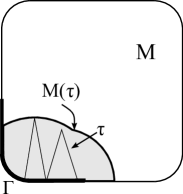
(a)

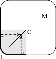
(b)

Fig. 1: (a) The domain of influence for a $\tau$ in $C(\overline{\Gamma})$ along with the profile of $\tau$. (b) The cut locus of $\Gamma$ along with a pair of equal length geodesics showing the break-down of the semi-geodesic coordinates at $\mathcal{C}$. The shaded region is the subset of $M$ that supports semi-geodesic coordinates.

We will use the following notions of volume: let $dV_{g}$ and $dS_{g}$ denote the Riemannian volume densities of $(M,g)$ and $(\partial M,g|_{\partial M})$ respectively. We remark that $dS_{g}$ is determined on $\Gamma$ by $\Lambda_{\Gamma}^{2T}$, see e.g. [13, Section 2.2] so we assume that it is known. We define the natural Riemannian volume density associated with $\Delta_{g,\mu}$ by $dV_{\mu}:=\mu dV_{g}$. We remark that its name derives from the fact that $\Delta_{g,\mu}$ is self-adjoint on $L^{2}(M;dV_{\mu})$ with domain $H_{0}^{1}(M)\cap H^{2}(M)$. The volume density $dV_{\mu}$ determines a volume measure which we denote $\operatorname{Vol_{\mu}}$. In addition, we will use the following shorthand notation for volumes of domains of influence $m(\tau):=\operatorname{Vol_{\mu}}(M(\tau))$.

We now describe a set of geometrically relevant subsets whose volumes will allow us to determine distances. Let $y\in\Gamma$, and let $s,h>0$ satisfy $s+h<\sigma_{\Gamma}(y)$. We define the wave cap,

$$\operatorname{cap}_{\Gamma}(y,s,h):=M(y,s+h)\setminus M^{\circ}(\Gamma,s),$$

where $M^{\circ}(\Gamma,s)=\{x\in M:d(x,\Gamma)<s\}$. Note that under the above hypotheses, $x(y,s)$ belongs to $\operatorname{cap}_{\Gamma}(y,s,h)$. We will use volumes of wave caps to determine distances.

Our main result is an algorithm to use the data $\Lambda_{\Gamma}^{2T}$ to construct distances of the form $r_{x(y,s)}(z)$ for $y,z\in\Gamma$ and $s>0$ with $d(x(y,s),z)<\min(\sigma_{\Gamma}(y),T)$. Our procedure can also be viewed as a constructive proof of the following known result, see e.g. [19]:

Theorem 1.

Let $y,z\in\Gamma$ and $s>0$ with $d(x(y,s),z)<\min(\sigma_{\Gamma}(y),T)$. Then $\Lambda_{\Gamma}^{2T}$ determines $r_{x(y,s)}(z)$.

The constructive proof will be given in Section 4. We note that this construction can also be viewed as a series of experiments. Following the proofs in Section 4.2, we provide an algorithmic overview of our distance computation procedure.

3 The Boundary Control method

In this section we describe the elements of the BC method required to determine $m(\tau)$ from $\Lambda_{\Gamma}^{2T}$. In addition, we briefly contrast our technique to alternative approaches to the BC method, and provide an overview of some computational aspects of the BC method.

The purpose of the BC method is to gain information about the interior of $M$ by processing boundary measurements for waves that propagate in $M$. To begin, we recall the control map, $W_{\tau}$, which takes a Neumann boundary source $f$ to the corresponding solution at time $T$. That is, let $\tau:\overline{\Gamma}\rightarrow[0,T]$ be continuous or a step function with open level sets and define,

$$W_{\tau}f:=u^{f}(T,\cdot),\quad W_{\tau}:L^{2}(S_{\tau})\rightarrow L^{2}(M).$$

The map $W_{\tau}$ is continuous, compact even, as a map from $L^{2}(S_{\tau})$ into $L^{2}(M)$, see e.g. [22, 36]. We will write $W:=W_{\tau}$ in the special case that $\tau\equiv T$, and we note that in this case, $S_{\tau}=(0,T)\times\Gamma$. Thus, for any other $\tau:\Gamma\rightarrow[0,T]$, $W_{\tau}$ can be viewed as a restriction of $W$ to sources supported in $S_{\tau}$.

One cannot directly observe the output of $W_{\tau}$ from boundary measurements because its output is a wave in the interior of $M$. Thus, in order to deduce information about the interior of $M$, one forms the connecting operator,

$$K_{\tau}:=W_{\tau}^{*}W_{\tau},\quad K:L^{2}(S_{\tau})\rightarrow L^{2}(S_{\tau}).$$

The continuity of $W_{\tau}$ implies that $K_{\tau}$ is a continuous operator on $L^{2}(S_{\tau})$. The practical utility of $K_{\tau}$ is that it can be computed by processing the boundary data, $\Lambda_{\Gamma}^{2T}$, see (6) below. This fact was first observed by Blagoveschenskii in the $1$+$1$-dimensional case [11]. We remark that $K_{\tau}$ derives its name from the fact that it connects the inner product on boundary sources with the inner product on waves in the interior. That is, for $f$, $h$ in $C_{0}^{\infty}(S_{\tau})$,

(5) $$(u^{f}(T,\cdot),u^{h}(T,\cdot))_{L^{2}(M;dV_{\mu})} =(f,Kh)_{L^{2}(S_{\tau};\,dt\otimes dS_{g})}.$$

We next recall the “Blagoveschenskii Identity,” which gives an expression for $K_{\tau}$ in terms of the data $\Lambda_{\Gamma}^{2T}$. In particular, we use the expression for $K_{\tau}$ appearing in [30],

(6) $$K_{\tau}=P_{\tau}\left(J\Lambda^{2T}_{\Gamma}\Theta-R\Lambda^{T}_{\Gamma}RJ\Theta\right)P_{\tau}.$$

Here, $\Theta:L^{2}((0,T)\times\Gamma)\rightarrow L^{2}((0,2T)\times\Gamma)$ is the inclusion (zero padding) given by:

$$\Theta f(t,\cdot):=\left\{\begin{array}[]{cl}f(t,\cdot)&0<t\leq T,\\ 0&T<t<2T,\end{array}\right.$$

$R:L^{2}((0,T)\times\Gamma)\rightarrow L^{2}((0,T)\times\Gamma)$ is the time reversal on $(0,T)$ given by:

$$Rf(t,\cdot):=f(T-t,\cdot)\quad 0<t<T,$$

$J:L^{2}((0,2T)\times\Gamma)\rightarrow L^{2}((0,T)\times\Gamma)$ is the time integration, given by:

$$Jf(t,\cdot):=\frac{1}{2}\int_{t}^{2T-t}f(s,\cdot)\,ds\quad 0<t<T,$$

and $P_{\tau}:L^{2}((0,T)\times\Gamma)\rightarrow L^{2}((0,T)\times\Gamma)$ is the orthogonal projection onto $L^{2}(S_{\tau})$ given by:

(7) $$P_{\tau}f:=1_{S_{\tau}}\cdot f.$$

We will use the special notation $K:=K_{\tau}$ when $\tau\equiv T$. In this case, the operator $P_{\tau}$ coincides with the identity and (5) can be written as $K=J\Lambda_{\Gamma}^{2T}\Theta-R\Lambda_{\Gamma}^{T}RJ\Theta$. Thus, for any $\tau$, the operator $K_{\tau}$ can be expressed as $K_{\tau}=P_{\tau}KP_{\tau}$.

3.1 Overview of BC method variants

There are several variants of the BC method, all of which are based on solving control problems of the form: Given a function $\phi$ on $M$, and a function $\tau:\overline{\Gamma}\rightarrow[0,T]$, find a boundary source $f$ such that

(8) $$W_{\tau}f=\phi.$$

In general, this problem is not solvable since the range of $W_{\tau}$ is generally not closed. On the other hand, it can be shown that approximate controllability holds, that is, there is a sequence $(f_{j})_{j=1}^{\infty}\subset C_{0}^{\infty}(S_{\tau})$ such that

(9) $$\lim_{j\to\infty}W_{\tau}f_{j}=1_{M(\tau)}\phi,\quad\text{in $L^{2}(M)$}.$$

The approximate controllability follows from the hyperbolic unique continuation result by Tataru [35] by a duality argument, see e.g. [19, p. 157].

The original version of the BC method [6] uses the Gram-Schmidt orthonormalization to find a sequence $(f_{j})_{j=1}^{\infty}$ satisfying (9). The method was implemented numerically in [5], and it requires choosing an initial system of boundary sources, see step 2 in [5, p. 233]. No constructive way to choose the initial boundary sources is given, and some choices may lead to an ill-conditioned orthonormalization process, see the discussion in [10].

More recently, Bingham, Kurylev, Lassas and Siltanen introduced a variant of the BC method where the Gram-Schmidt process is replaced by a quadratic optimization [10]. Their method is posed in the case $\Gamma=\partial M$, and is based on constructing a sequence $(f_{j})_{j=1}^{\infty}$ such that the limit (9) becomes focused near a point. To elaborate, their method considers an arbitrary $h\in L^{2}((0,T)\times\partial M)$ with $\phi$ chosen as $\phi=Wh$. For a point $y\in\partial M$ and small enough $0<s,r<T$, they choose appropriate $\tau$ to produce a sequence of sources $(f_{j})_{j=1}^{\infty}\subset S_{\tau}$ such that $Wf_{j}\rightarrow 1_{\operatorname{cap}_{\partial M}(y,s,r)}Wh$. However, no constructive procedure to choose the boundary source $h$ is given, and some choices may lead to sequences such that this limit vanishes also near the point where it should be focused, see the assumption on the non-vanishing limit in [10, Corollary 2]. We note that the method [10] has not been implemented numerically.

Our approach employs a quadratic optimization similar to [10] but differs from it by selecting $\phi=1$ in place of $Wh$. By solving the approximate control problems for this choice of $\phi$, we can compute volumes $m(\tau)$ for certain functions $\tau:\overline{\Gamma}\to[0,T]$. We note that the method we use to compute these volumes was developed in [28, 29], and it was applied to an inverse obstacle problem in [30]. Here we show how to compute the boundary distance functions from the volumes $m(\tau)$.

Our method contains only constructive choices of boundary sources, and it allows us to understand the numerical errors that we make in each step of the algorithm. In Section 5, we see that the dominating source of error in our numerical examples is related to the instability of the control problem (8) under the constraint $\mathop{\operator@font supp}\nolimits(f)\subset S_{\tau}$. This instability is inherent in all the variants of the BC method mentioned above.

In addition to [5], the only multidimensional implementation of a variant of the BC method, that we are aware of, is [31]. This variant is based on solving the control problem (8) without the constraint $\mathop{\operator@font supp}\nolimits(f)\subset S_{\tau}$. The target function $\phi$ is chosen to be harmonic, and the method exploits the density of products of harmonic functions in $L^{2}(M)$. Such an approach works only in the isotropic case, that is, in the case of the wave equation $\partial_{t}^{2}-c(x)^{2}\Delta$ where the sound speed $c(x)>0$ is scalar valued.

We also mention that the original version of the BC method [6] assumes the wave equation to be isotropic, and that in [24], an approach similar to [31] was shown to recover a lowpass version of the sound speed in a Lipschitz stable manner under additional geometric assumptions. Furthermore, we refer to [18] for a comparison of the BC method and other inversion methods in the $1$+$1$-dimensional case.

3.2 Regularized estimates of volumes of domains of influence

We now explain how we pose our approximate control problems, and how we use their solutions to compute volumes of domains of influence. To begin, let $\tau:\overline{\Gamma}\rightarrow[0,T]$ be either a step function with open level sets or $\tau\in C(\overline{\Gamma})$. We obtain an approximate solution to (8) with right-hand side $\phi=1$, by solving the following minimization problem: for $\alpha>0$ let

(10) $$f_{\alpha}:=\operatorname*{argmin}_{f\in L^{2}(S_{\tau})}\|u^{f}(T,\cdot)-1\|_{L^{2}(M;dV_{\mu})}^{2}+\alpha\|f\|_{L^{2}(S_{\tau};dt\otimes dS_{g})}^{2}.$$

As was shown in [28], for $\tau$ as above: this problem is solvable, the solution can be obtained by solving a linear problem involving $K_{\tau}$, and $u^{f_{\alpha}}(T,\cdot)\rightarrow 1_{M(\tau)}$ as $\alpha\rightarrow 0$. For the convenience of the reader, we outline the proof here, and moreover, we recall that the approximate control solutions, $f_{\alpha}$, can be used to compute $m(\tau)$.

To show that (10) has a solution we first recall two results about Tikhonov regularization. For proofs see e.g. [21, Th. 2.11] and [30], respectively.

Lemma 2.

Suppose that $X$ and $Y$ are Hilbert spaces. Let $y\in Y$ and let $A:X\to Y$ be a bounded linear operator. Then for all $\alpha>0$ there is a unique minimizer of

$$\left\|Ax-y\right\|^{2}+\alpha\left\|x\right\|^{2}$$

given by $x_{\alpha}=(A^{*}A+\alpha)^{-1}A^{*}y$.

Lemma 3.

Suppose that $X$ and $Y$ are Hilbert spaces. Let $y\in Y$ and let $A:X\to Y$ be a bounded linear operator with range $R(A)$. Then $Ax_{\alpha}\to Qy$ as $\alpha\to 0$, where $x_{\alpha}=(A^{*}A+\alpha)^{-1}A^{*}y$, $\alpha>0$, and $Q:Y\to\overline{R(A)}$ is the orthogonal projection.

Since $W_{\tau}$ is bounded, the first Lemma implies that (10) is solvable. To apply the second lemma to our current setting, we must describe the range of $W_{\tau}$ and compute $W_{\tau}^{*}1$. Toward that end, we recall that $\mathop{\operator@font supp}\nolimits(W_{\tau}f)\subset M(\tau)$ by finite speed of propagation. When $\tau$ is a step function, Tataru’s unique continuation [35] implies that the inclusion

(11) $$\{W_{\tau}f;\ f\in L^{2}(S_{\tau})\}\subset L^{2}(M(\tau)),$$

is dense, see e.g. [19, Th. 3.10]. The result was extended to the case of $\tau\in C(\overline{\Gamma})$ in [28]. Thus $\overline{R(W_{\tau})}=L^{2}(M(\tau))$ for the functions $\tau$ under consideration. To compute $W_{\tau}^{*}1$, we note an equality similar to (5) that is satisfied for $f\in L^{2}(S_{\tau})$:

(12) $$(u^{f}(T,\cdot),1)_{L^{2}(M;dV_{\mu})}=(f,P_{\tau}b)_{L^{2}((0,T)\times\partial M;dt\otimes dS_{g})}.$$

Here, $P_{\tau}$ is defined by (7), and $b(t,x):=T-t$ for $(t,x)\in(0,T)\times\Gamma$. Thus, $W_{\tau}^{*}1=P_{\tau}b$.

Applying Lemmas 2 and 3 to the observations above, we see that for each $\alpha>0$, equation (10) has a unique solution $f_{\alpha}$, given by:

(13) $$f_{\alpha}:=(W_{\tau}^{*}W_{\tau}+\alpha)^{-1}W_{\tau}^{*}1=(K_{\tau}+\alpha)^{-1}P_{\tau}b,$$

thus $f_{\alpha}$ is obtained from the data. Moreover, the waves $W_{\tau}f_{\alpha}$ satisfy $W_{\tau}f_{\alpha}\to Q_{\tau}1$ in $L^{2}(M)$ as $\alpha$ tends to zero, where $Q_{\tau}$ is the projection of $L^{2}(M)$ onto the subspace $\overline{R(W_{\tau})}=L^{2}(M(\tau))$. Note that $Q_{\tau}1=1_{M(\tau)}$. Using this fact and applying (12) to $f_{\alpha}$ we conclude,

(14) $$m(\tau)=\lim_{\alpha\to 0+}(f_{\alpha},P_{\tau}b)_{L^{2}((0,T)\times\partial M;dt\otimes dS_{g})}.$$

Thus we can compute $m(\tau)$ from operations performed on the data $\Lambda^{2T}_{\Gamma}$.

4 Constructing distances

In this section, we present our proof of Theorem 1. We accomplish this through a sequence of lemmas that are designed to illuminate the steps required to turn the theorem into an algorithm. In addition, we provide an alternative technique to determine distances, which we use in our computational implementation.

4.1 Constsructive proof of Theorem 1

The following lemma provides a bound on the distance between a point and a wave-cap,

Lemma 4.

Let $y\in\Gamma$, $s\in(0,\sigma_{\Gamma}(y))$, and $h\in(0,\sigma_{\Gamma}(y)-s)$. Let $z\in\Gamma$ and $r>0$. Then $d(z,\operatorname{cap}_{\Gamma}(y,s,h))<s+r$ if and only if

(15) $$m(s1_{\Gamma}+r1_{z}+h1_{y})-m(s1_{\Gamma}+r1_{z})<m(s1_{\Gamma}+h1_{y})-m(s1_{\Gamma}).$$

We note that (15) tests whether there is an overlap between the sets $\operatorname{cap}_{\Gamma}(y,s,h)$ and $\operatorname{cap}_{\Gamma}(y,s,r)$, see Figure 2a.

Proof.

As $h>0$ and $h<\sigma_{\Gamma}(y)-s$, we see that $\operatorname{cap}_{\Gamma}(y,s,h)$ contains a non-empty open set. In particular, it has strictly positive measure. Moreover, if $d(z,\operatorname{cap}_{\Gamma}(y,s,h))<s+r$ then the intersection of $\operatorname{cap}_{\Gamma}(y,s,h)$ and $M(z,s+r)$ contains a non-empty open set and has strictly positive measure.

Notice that $m(s1_{\Gamma}+h1_{y})$ is the measure of $M(y,s+h)\cup M(\Gamma,s)$ and that $m(s1_{\Gamma}+h1_{y})-m(s1_{\Gamma})$ is the measure of $\operatorname{cap}_{\Gamma}(y,s,h)$. Indeed,

$$\operatorname{Vol_{\mu}}(M(y,s+h)\cup M(\Gamma,s)) =\operatorname{Vol_{\mu}}((M(y,s+h)\cup M(\Gamma,s))\setminus M(\Gamma,s))$$

$$\quad+\operatorname{Vol_{\mu}}(M(\Gamma,s))$$

$$=\operatorname{Vol_{\mu}}(\operatorname{cap}_{\Gamma}(y,s,h))+\operatorname{Vol_{\mu}}(M(\Gamma,s)).$$

Analogously, $m(s1_{\Gamma}+r1_{z}+h1_{y})-m(s1_{\Gamma}+r1_{z})$ is the measure of

$$M(y,s+h)\setminus(M(\Gamma,s)\cup M(z,s+r))=\operatorname{cap}_{\Gamma}(y,s,h)\setminus M(z,s+r).$$

If $d(z,\operatorname{cap}_{\Gamma}(y,s,h))<s+r$ then the intersection of $\operatorname{cap}_{\Gamma}(y,s,h)$ and $M(z,s+r)$ has strictly positive measure, whence (15) holds.

On the other hand, if $d(z,\operatorname{cap}_{\Gamma}(y,s,h))\geq s+r$ then $\operatorname{cap}_{\Gamma}(y,s,h)\cap M(z,s+r)$ is contained in the topological boundary of $M(z,s+r)$ which is of zero measure [28]. Thus

$$m(s1_{\Gamma}+r1_{z}+h1_{y})-m(s1_{\Gamma}+r1_{z})=m(s1_{\Gamma}+h1_{y})-m(s1_{\Gamma}),$$

and (15) does not hold.   ∎

[1.5in]

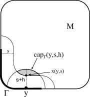
(a)

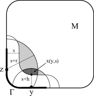
(a) $s+r>d(z,\operatorname{cap}_{\Gamma}(y,s,h))$

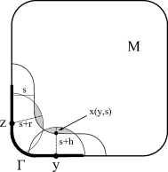
(b) $s+r\leq d(z,\operatorname{cap}_{\Gamma}(y,s,h))$

Fig. 3: The light gray regions indicate the wave caps used in Lemma 4 and the dark gray region indicates the overlap between the caps.

Fig. 2: A wave cap

[3.6in]

The next lemma demonstrates that when $s<\sigma_{\Gamma}(y)$, the wave caps $\operatorname{cap}_{\Gamma}(y,s,h)$ tend, in a set-theoretic sense, towards $x(y,s)$.

Lemma 5.

Let $y\in\Gamma$ and $s\in(0,\sigma_{\Gamma}(y))$. Then,

(16) $$\bigcap_{h>0}\operatorname{cap}_{\Gamma}(y,s,h)=\{x(y,s)\}.$$

Proof.

Let $y,s$ as above, and let $I(y,s)$ denote the left hand side of (16). Let $w$ be any point belonging to $I(y,s)$. Then $w\in\operatorname{cap}_{\Gamma}(y,s,h)$ for all $h>0$, so $s\leq d(\Gamma,w)$ and $d(y,w)<s+h$ for all $h>0$, thus $d(y,w)\leq s$. Since $y\in\Gamma$, we conclude $s=d(\Gamma,w)=d(y,w)$. On the other hand, if $w$ is a point in $M$ satisfying $s=d(\Gamma,w)=d(y,w)$, then $w\in\operatorname{cap}_{\Gamma}(y,s,h)$ for any $h>0$, hence $w\in I(y,s)$. We conclude,

(17) $$I(y,s)=\{w\in M:d(y,w)=d(\Gamma,w)=s\}.$$

Because $s<\sigma_{\Gamma}(y)$, we have $d(x(y,s),y)=d(x(y,s),\Gamma)=s$, so $x(y,s)\in I(y,s)$. It remains to show that no other points belong to $I(y,s)$.

Let $w$ belong to $I(y,s)$, we will show that $w=x(y,s)$. If we knew for certain that $w$ belonged to the image of the semi-geodesic coordinates, then this would be immediate from the definition of these coordinates. On the other hand, if we did not require $\Gamma$ to be open, then simple examples show that for points $y$ in the topological boundary of $\Gamma$ it is possible that $I(y,s)$ has many points. We demonstrate that when $\Gamma$ is open this cannot happen.

Since $M$ is a compact connected metric space with distance arising from a length function, the Hopf-Rinow theorem for length spaces applies and we conclude that there is a minimizing path $\beta:[0,l]\rightarrow M$ from $y$ to $w$. By [2], $\beta$ is $C^{1}$ and we may assume that it is unit speed parameterized. Hence $l=s$. As $\beta$ is minimizing from both $y$ and $\Gamma$ to $w$, we see that $\dot{\beta}(0)=\nu$. Thus $\beta$ coincides with $x(y,t)$ for $t\leq\min(s,\tau_{M}(y,\nu))$. But $s<\sigma_{\Gamma}(y)$, hence $s<\tau_{M}(y,\nu)$. Thus we see that $w=\beta(s)=x(y,s)$.   ∎

We use the preceding lemma to show that, when $h$ is small, the distance between a point $z\in\Gamma$ and the wave cap $\operatorname{cap}_{\Gamma}(y,s,h)$ surrounding $x(y,s)$ yields an approximation to $d(z,x(y,s))$. We depict this approximation in Figure 4.

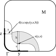
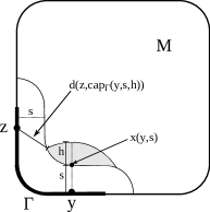
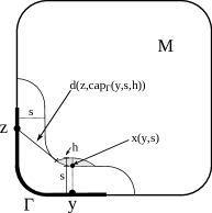
Fig. 4: Cartoon demonstrating that $d(z,\operatorname{cap}_{\Gamma}(y,s,h))\rightarrow d(z,x(y,s))$ as $h\rightarrow 0$.

Lemma 6.

For $y,z\in\Gamma$, and $s<\sigma_{\Gamma}(y)$, $d(z,\operatorname{cap}_{\Gamma}(y,s,h))\rightarrow d(z,x(y,s))$ as $h\rightarrow 0$.

Proof.

Let $\{h_{j}\}\subset\mathbb{R}_{+}$ be a sequence for which $h_{j}\downarrow 0$. Then each $\operatorname{cap}_{\Gamma}(y,s,h_{j})$ is compact, so there exists $w_{j}\in\operatorname{cap}_{\Gamma}(y,s,h_{j})$ such that $d(z,w_{j})=d(z,\operatorname{cap}_{\Gamma}(y,s,h_{j}))$. Because $M$ is a compact manifold, the sequence $\{w_{j}\}$ has a convergent subsequence $\{w_{j_{k}}\}$ converging to a point $w$. Since the wave caps $\operatorname{cap}_{\Gamma}(y,s,h)$ nest, the tail of $\{w_{j_{k}}\}$ belongs to the closed set $\operatorname{cap}_{\Gamma}(y,s,h_{j_{k}})$ for each $j_{k}$, hence $w\in\operatorname{cap}_{\Gamma}(y,s,h)$ for each $h>0$. By the previous lemma, we conclude $w=x(y,s)$.

Together, continuity of the distance function and the particular choice of the $w_{j_{k}}$ imply that, $d(z,\operatorname{cap}_{\Gamma}(y,s,h_{j_{k}}))=d(z,w_{j_{k}})\rightarrow d(z,x(y,s)).$ Since the wave caps nest, the sequence $\{d(z,w_{j})\}$ is monotone non-decreasing, and since it is bounded above it has a limit. In particular, any subsequential limit coincides with the limit. Thus we conclude that $d(z,\operatorname{cap}_{\Gamma}(y,s,h_{j}))\rightarrow d(z,x(y,s))$ as $j\rightarrow\infty$, and in turn, $d(z,\operatorname{cap}_{\Gamma}(y,s,h))\rightarrow d(z,x(y,s))$ as $h\rightarrow 0$.   ∎

The volumes appearing in Lemma 4 cannot be computed directly with the $\tau$’s appearing in the regularized volume determination. That is, the lemma requires us to compute volumes such as $m(s1_{\Gamma}+r1_{z}+h1_{y})$, but the function $\tau=s1_{\Gamma}+r1_{z}+h1_{y}$ is equivalent to $s1_{\Gamma}$ in $L^{2}((0,T)\times\Gamma)$. As a result, the set $L^{2}(S_{\tau})$ will produce waves that fill $L^{2}(M(s1_{\Gamma}))$ as opposed to the desired set $L^{2}(M(\tau))$. The problem is that the spikes $h1_{y}$ and $r1_{z}$ have supports with $dS_{g}$ measure zero. The remedy is to replace the spikes by functions that produce the same domains of influence but have better supports. To accomplish this, for $y\in\Gamma$ and $R\in[0,\infty)$, we define $\tau_{y}^{R}$ on $\Gamma$ by:

(18) $$\tau_{y}^{R}(z):=R-d(z,y)\text{\quad for $z\in\Gamma$}.$$

Note that $\tau_{y}^{R}$ is continuous. We recall that under Assumption 2 the distances $d(y,z)$ for $y,z\in\Gamma$ with $d(y,z)<T$ are known (or, alternatively, that they have been computed in some other fashion from $\Lambda_{\Gamma}^{2T}$). Thus under our assumptions the functions $\tau_{y}^{R}$ are known.

Lemma 7.

Let $y,z\in\Gamma$, $s,r,h>0$. We will use the notation $f\vee g$ to denote the function obtained by taking the pointwise maximum of $f$ and $g$. Then, we have the following equalities,

(19) $$M(\tau_{y}^{r}) =M(r1_{y}),$$

(20) $$M(\tau_{y}^{s+h}\vee\tau_{z}^{s+r}\vee s) =M(h1_{y}+r1_{z}+s1_{\Gamma}),$$

(21) $$M(\tau_{z}^{s+r}\vee s) =M(s1_{\Gamma}+r1_{z}).$$

Proof.

Let $x\in M(r1_{y})$, then $d(y,x)<r$. Since $\tau_{y}^{r}(y)=r$, we have that $d(y,x)<\tau_{y}^{r}(x)$, hence $x\in M(\tau_{y}^{r})$. Now let $x\in M(\tau_{y}^{r})$. Then there is a point $z\in\Gamma$ for which $d(x,z)<\tau_{y}^{r}(z)$. Applying the definition of $\tau_{y}^{r}$, we find $r>d(x,z)+d_{\Gamma}(y,z)\geq d(x,z)+d(y,z)\geq d(x,y)$. Hence $x\in M(r1_{y})$. We conclude that $M(\tau_{y}^{r})=M(r1_{y})$.

We demonstrate equality (20) and note that (21) is proved in an analogous fashion. Let $\tau=\tau_{y}^{s+h}\vee\tau_{z}^{s+r}\vee s$. Then $x\in M(\tau)$ just in case $d(x,p)<\tau(p)$ for some $p\in\Gamma$, which happens if and only if $d(x,p)$ is less than $\tau_{y}^{s+h}(p),\tau_{z}^{r+h}(p)$, or $s$. The preceding paragraph implies that this happens just in case $x$ belongs to $M((s+h)1_{y}),M((s+r)1_{z}),$ or $M(s1_{\Gamma})$, which happens if and only if $x\in M(s1_{y}+r1_{z}+s1_{\Gamma})$.   ∎

We are finally in a position to prove Theorem 1.

Proof. [Of Theorem 1] First, let $r$ and $h$ be positive numbers satisfying $s+r<T$ and $s+h<T$. Define functions $\tau_{1}=s$, $\tau_{2}=\tau_{y}^{s+h}\vee s$, $\tau_{3}=\tau_{z}^{s+r}\vee s$, and $\tau_{4}=\tau_{y}^{s+h}\vee\tau_{z}^{s+r}\vee s$. Using the regularized volume determination from equation (14), we compute the volumes $m(\tau_{i})$ for $i=1,\ldots,4$. Then, Lemma 7 implies that $m(\tau_{1})=m(s1_{\Gamma})$, $m(\tau_{2})=m(s1_{\Gamma}+h1_{y})$, $m(\tau_{3})=m(s1_{\Gamma}+r1_{z})$, and $m(\tau_{4})=m(s1_{\Gamma}+h1_{y}+r1_{z})$, thus we have determined the volumes appearing in (15). By Lemma 4 we can compute $d(z,\operatorname{cap}_{\Gamma}(y,s,h))$ by

(22) $$d(z,\operatorname{cap}_{\Gamma}(y,s,h))=s+\inf\{r:0\leq r<T-s,\text{ and (\ref{eqn:VolumeComparison}) holds\}}.$$

Finally, by Lemma 6, we can compute $d(z,x(y,s))$ by

(23) $$d(z,x(y,s))=\lim_{h\rightarrow 0}d(z,\operatorname{cap}_{\Gamma}(y,s,h)).\qquad\end@proof$$

4.2 Alternative distance estimation method

The method to estimate distances derived from Theorem 1 uses the fact that, under the hypotheses of the theorem, the distance between a point $z\in\Gamma$ and the wave cap $\operatorname{cap}_{\Gamma}(y,s,h)$ serves as an approximation to $d(z,x(y,s))$, and that this approximation improves as $h\rightarrow 0$. However, in the case where $g$ is the Euclidean metric, $d(z,\operatorname{cap}_{\Gamma}(y,s,h))$ converges to $d(z,x(y,s))$ with the rate $\mathcal{O}(h^{1/2})$. Thus the convergence is typically slow. In this section, we provide another technique to estimate the distance to points which we find, for a given nonzero $h$, tends to provide better distance estimates.

The idea of this alternative distance estimation method is to once again check for overlap between the sets $\operatorname{cap}_{\Gamma}(y,s,h)$ and $\operatorname{cap}_{\Gamma}(z,s,r)$, but instead of seeking the minimum $r$ for which these wave caps overlap, we seek $r$ for which $\operatorname{Vol_{\mu}}(\operatorname{cap}_{\Gamma}(y,s,h)\cap\operatorname{cap}_{\Gamma}(z,s,r))$ is half of $\operatorname{Vol_{\mu}}(\operatorname{cap}_{\Gamma}(y,s,h))$.

Before proving that our alternative distance estimation procedure is valid, we provide a lemma that shows that the diameter of a wave cap vanishes as the height of the cap goes to zero.

Lemma 8.

Let $y,z\in\Gamma$, $s\in(0,\sigma_{\Gamma}(y))$. Then,

(24) $$\lim_{h\rightarrow 0}\operatorname{diam}(\operatorname{cap}(y,s,h))=0.$$

Proof.

Suppose the claim were false. Then there exists a sequence of positive real numbers $h_{i}\downarrow 0$ and points $p_{i}\in\operatorname{cap}_{\Gamma}(y,s,h_{i})$ such that $d(x(y,s),p_{i})\not\rightarrow 0$. Since $M$ is compact, the sequence $\{p_{i}\}$ has a convergent subsequence. Relabeling this subsequence by $p_{i}$ we have that there exists $p\in M$ such that $p_{i}\rightarrow p$. But this implies that $d(p,x(y,s))\neq 0$, hence $p\neq x(y,s)$. On the other hand, since $p_{i}\in\operatorname{cap}_{\Gamma}(y,s,h_{i})$ we must have that $p\in\bigcap_{h>0}\operatorname{cap}_{\Gamma}(y,s,h)$, but this gives a contradiction, since by Lemma 5 this implies that $p=x(y,s)$.   ∎

We now present our alternative distance estimation method.

Lemma 9.

Let $y,z\in\Gamma$, $s\in(0,\sigma_{\Gamma}(y))$, and $0<h<\sigma_{\Gamma}(y)-s$. Let $r_{h}$ be the solution to,

(25) $$\operatorname{Vol_{\mu}}(\operatorname{cap}_{\Gamma}(y,s,h)\cap\operatorname{cap}_{\Gamma}(z,s,r_{h}))=\frac{1}{2}\operatorname{Vol_{\mu}}(\operatorname{cap}_{\Gamma}(y,s,h)).$$

Then, for $d_{h}:=s+r_{h}$, we have that $d_{h}\rightarrow d(z,x(y,s))$ as $h\rightarrow 0$.

Proof.

First, we recall that for $s$ and $h$ as above, $\operatorname{cap}_{\Gamma}(y,s,h)$ will contain a non-empty open set, hence the right-hand side of (25) will be nonzero. Thus, from the definition of $r_{h}$, we conclude that $\operatorname{cap}_{\Gamma}(y,s,h)\cap\operatorname{cap}_{\Gamma}(z,s,r_{h})$ is a non-empty and proper subset of $\operatorname{cap}_{\Gamma}(y,s,h)$. Using the definition of $\operatorname{cap}_{\Gamma}(z,s,r_{h})$ and $r_{h}$ we conclude that $s+r_{h}\geq d(z,\operatorname{cap}_{\Gamma}(y,s,h))$. On the other hand, since the intersection between the wave caps is a proper subset of $\operatorname{cap}_{\Gamma}(y,s,h)$ we see that there exists $p\in\operatorname{cap}_{\Gamma}(y,s,h)\setminus\operatorname{cap}_{\Gamma}(z,s,r_{h})$. In particular, this implies that $s+r_{h}\leq d(z,p)\leq\operatorname{dist}(z,\operatorname{cap}_{\Gamma}(y,s,h))+\operatorname{diam}(\operatorname{cap}_{\Gamma}(y,s,h))$. Hence,

$$d(z,\operatorname{cap}_{\Gamma}(y,s,h))\leq d_{h}\leq d(z,\operatorname{cap}_{\Gamma}(y,s,h))+\operatorname{diam}(\operatorname{cap}_{\Gamma}(y,s,h)).$$

Since $d(z,\operatorname{cap}_{\Gamma}(y,s,h))\rightarrow d(z,x(y,s))$ and $\operatorname{diam}(\operatorname{cap}_{\Gamma}(y,s,h))\rightarrow 0$ as $h\rightarrow 0$, we conclude that $d_{h}\rightarrow d(z,x(y,s))$ as $h\rightarrow 0$.   ∎

We summarize the steps of the proof in an algorithmic form in Algorithm 1.

let: $y,z\in\Gamma$ and $s>0$ with $r_{x(y,s)}(z)<T.$

let: $h_{0}>0$ small enough that $s+h_{0}<\min\{\sigma_{\Gamma}(y),T\}$.

for $0<h<h_{0}$:

       for $0<r<T-s$:

             let: $\tau_{1}=s1_{\Gamma}$, $\tau_{2}=\tau_{y}^{s+h}$, $\tau_{3}=\tau_{z}^{s+r}$, $\tau_{4}=\tau_{1}\vee\tau_{2}\vee\tau_{3}$

             for $\alpha>0$:

                   for $i=1,\ldots,4$:

                         let: $f_{\alpha,i}$ solve:

$$(K_{\tau_{i}}+\alpha)P_{\tau_{i}}f=P_{\tau_{i}}b$$

                        

                  

                  

            

             for $i=1,\ldots,4$:

                   compute:

$$m(\tau_{i})=\lim_{\alpha\rightarrow 0}(f_{\alpha,i},b)_{L^{2}(S_{\tau};\,dt\otimes dS_{g,\mu})}$$

                  

            

             compute:

$$\begin{array}[]{rcl}m_{\text{target cap}}(h)&:=&m(\tau_{2})-m(\tau_{1})\\ m_{\text{overlap}}(h,r)&:=&m(\tau_{4})-m(\tau_{3})-m(\tau_{2})+m(\tau_{1})\\ \end{array}$$

            

      

       compute: $r_{h}$ by either:

method 1: let $r_{h}$ satisfy:

$$r_{h}=\inf\{r>0:m_{\text{overlap}}(h,r)>0\}.$$

      method 2: let $r_{h}$ be the solution to:

$$m_{\text{overlap}}(h,r)=\frac{1}{2}m_{\text{target cap}}(h).$$

      

compute: $r_{x(y,s)}(z)$ by:

$$r_{x(y,s)}(z)=s+\lim_{h\rightarrow 0}r_{h}.$$

Algorithm 1 Continuum level description of distance determination algorithm.

5 Computational experiment

In this section we present a numerical example that demonstrates the distance determination procedure that we have described in the previous sections. For computational simplicity, we demonstrate our procedure in the Euclidean setting. However, we stress that our method can be applied in the general Riemannian setting.

5.1 Numerical method for the direct problem

For our numerical example, we take the manifold $M$ to be the $2$-dimensional Euclidean lower half-space equipped with the canonical metric and a unit weight function, $\mu\equiv 1$. Under these particular choices, the weighted Laplace-Beltrami operator reduces to the Euclidean $2$-dimensional Laplacian. Hence, for our example, the Riemannian wave equation (1) simplifies to the standard $2+1$-dimensional wave equation with constant sound-speed, $c\equiv 1$. In order to simulate the situation of partial, local illumination, for our source/receiver set, $\Gamma$, we take $\Gamma=[-L,L]\times\{0\}\subset\partial M$ with $L=2.232$. We simulate waves propagating for $2T$ time units, where $T=1.249$.

For sources, we use a basis of Gaussian pulses with the form

$$\varphi_{i,j}(t,x)=C\exp\left(-a_{t}(t-t_{i})^{2}-a_{x}(x-x_{j})^{2}\right),$$

with parameters $a_{t}=a_{x}=4\cdot 10^{3}$, and where we have selected the constant $C$ to normalize the $\varphi_{i,j}$. Sources are applied on the regular grid:

$$\left\{(t_{s,i},(x_{s,j},0)):\begin{array}[]{ll}t_{s,i}=t_{s,1}+(i-1)\Delta t_{s}&i=1,\ldots,N_{t,s},\\ x_{s,j}=x_{s,1}+(j-1)\Delta x_{s}&j=1,\ldots,N_{x,s}\end{array}\right\},$$

where the source offset $\Delta x_{s}$ and time between source applications $\Delta t_{s}$ are both selected as $\Delta x_{s}=\Delta t_{s}=.0147$. At each of the $N_{x,s}=309$ source positions we apply $N_{t,s}=78$ sources. For each basis function, we record the Dirichlet trace data on the regular grid:

$$\left\{(t_{r,l},(x_{r,k},0)):\begin{array}[]{ll}t_{r,l}=t_{r,1}+(l-1)\Delta t_{r}&l=1,\ldots,N_{t,r},\\ x_{r,k}=x_{r,1}+(k-1)\Delta x_{r}&k=1,\ldots,N_{x,r}\end{array}\right\}.$$

The receiver offset $\Delta x_{r}$ has been taken to be half the source offset, resulting in $N_{x,r}=633$ receiver positions. The time between receiver measurements, $\Delta t_{r}$, is $1/10$ the source time between source applications, resulting in $N_{t,r}=1701$ receiver measurements at each receiver position.

We discretize the Neumann-to-Dirichlet map by solving the forward problem for each source $\varphi_{i,j}$ and recording its Dirichlet trace at the receiver positions and times described above. That is, we compute the following data,

(26) $$\left\{\Lambda^{2T}\varphi_{i,j}(t_{r,l},x_{r,k})=u^{\varphi_{i,j}}(t_{r,l},x_{r,k}):\begin{array}[]{l}i=1,\ldots,N_{t,s},~{}j=1,\ldots,N_{x,s},\\ l=1,\ldots,N_{t,r},~{}k=1,\ldots,N_{x,r}\end{array}\right\}.$$

To perform the forward modelling, we use the continuous Galerkin finite element method with piecewise linear Lagrange polynomial elements and implicit Newmark time-stepping. In particular, we use the FEniCS package [25]. We use a regular triangular mesh, where the time step and mesh spacing are selected so that $8$ points per wavelength (in directions parallel to the grid axes) are used at the frequency $f_{0}$ where the spectrum of the temporal portion of the source falls below $10^{-6}$ times its maximum value.

5.2 Solving the control problem

We discretize the connecting operator $K$ by approximating its action as an operator on $\operatorname{span}\{\varphi_{i,j}\}$. That is, we use the discrete Neumann-to-Dirichlet data, (26), to discretize $K_{\tau}$ by formula (6), where $\tau\equiv T$. To be specific, we first compute the Gram matrix $[G]_{ij}=(\varphi_{i},\varphi_{j})$ and its inverse $[G^{-1}]$, and then compute the matrices for the operators $J\Lambda_{\Gamma}^{2T}$, $R\Lambda_{\Gamma}^{T}$ and $RJ$ acting on $\operatorname{span}\{\varphi_{i,j}\}$ as follows:

$$[J\Lambda_{\Gamma}^{2T}]_{ij} =\sum_{k}[G^{-1}]_{ik}(\varphi_{k},J\Lambda_{\Gamma}^{2T}\varphi_{j}),$$

$$[R\Lambda_{\Gamma}^{T}]_{ij} =\sum_{k}[G^{-1}]_{ik}(\varphi_{k},R\Lambda_{\Gamma}^{T}\varphi_{j}),$$

$$[RJ]_{ij} =\sum_{k}[G^{-1}]_{ik}(\varphi_{k},RJ\varphi_{j}).$$

Using these operators we can compute the matrix for $K$,

(27) $$[K]=[J\Lambda_{\Gamma}^{2T}]-[R\Lambda_{\Gamma}^{T}][RJ].$$

In Table 1 we demonstrate the effect of the constituent matrices in (27) on a source $f$ and how these combine to form $Kf$.

(a)
(b)
(c)
(d)
(e)

Table 1: Demonstration of the action of the operators appearing in (27), (a) a source $f$, (b) $RJf$, (c) $R\Lambda_{\Gamma}^{T}RJf$, (d) $J\Lambda_{\Gamma}^{2T}f$, and (e) $Kf$. Note that all plots are on the function level, and each function depicted was obtained from coefficients that were computed as described in Section 5.2.

For $\tau\in C(\Gamma)$, with $0\leq\tau\leq T$, we obtain the matrix $[K_{\tau}]$ discretizing the connecting operator $K_{\tau}$ by masking the entries in $[K]$ that correspond to basis functions $\varphi_{i,j}$ with centers $(t_{s,i},x_{s,j})\not\in S_{\tau}$. We note that, in practice, we find that this tends to provide a better approximation to $K_{\tau}$ than computing the matrix $[P_{\tau}]$ and computing the product $[P_{\tau}][K][P_{\tau}]$.

We consider the discretized control problem

(28) $$([K_{\tau}]+\alpha[P_{\tau}])[f_{\alpha}]=[P_{\tau}][b],$$

where we use the matrix $[P_{\tau}]$ to refer to the mask described above, and use $\alpha=10^{-5}$. Recall that $b$ is the function given by $b(t,x)=T-t$, as defined beneath (12). To solve (28) for $[f_{\alpha}]$, we use restarted GMRES. In Figure 5 and Table 2 we depict control solutions $f_{\alpha}=\sum_{i}[f_{\alpha}]_{i}\varphi_{i}$ and their associated wavefields $u^{f_{\alpha}}(T,\cdot)$. A volume estimate $\hat{m}(\tau)$ for $m(\tau)$ is obtained from $[f_{\alpha}]$ by computing the discretized inner product $\hat{m}(\tau)=[f_{\alpha}]^{T}[G][b]$, which approximates $m(\tau)$ as in (14). For the remainder of this paper we will continue to use the notation $\hat{m}(\tau)$ to indicate the approximation to $m(\tau)$ computed in this fashion.

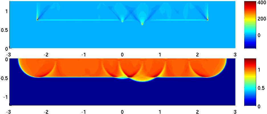
Fig. 5: Illustration of a source $f_{\alpha}$ and the corresponding wavefield $u^{f_{\alpha}}(T,\cdot)$ for which $u^{f_{\alpha}}(T,\cdot)\approx 1_{M(\tau)}$. Here, $\tau$ corresponds to $\tau_{4,1}$ from Table 2. Note that, to show both plots with the same horizontal axis, we have extended $f_{\alpha}$ to zero outside of $[0,T]\times\Gamma$.

5.3 Estimating distances

$\tau$	$f_{\alpha}$	$u^{f_{\alpha}}(T,\cdot)$
$\tau_{1}$
$\tau_{2}$
$\tau_{3,1}$
$\tau_{4,1}$
$\tau_{3,2}$
$\tau_{4,2}$
$\tau_{3,3}$
$\tau_{4,3}$

Table 2: Illustration of the essential features of sources and waves used in distance estimation procedure. Solutions, $f_{\alpha}$, to the discretized control problem plotted next to their associated wavefields $u^{f_{\alpha}}(T,\cdot)$ approximating $1_{M(\tau)}$. Plotted for $\tau$ of the form $\tau_{1}=s1_{\Gamma}$, $\tau_{2}=\tau_{y}^{s+h}$, $\tau_{3,j}=\tau_{z}^{s+r_{j}}$, and $\tau_{4,j}=\tau_{1}\vee\tau_{2}\vee\tau_{3,j}$, where $y=(0,0)$, $z=(0.529,0)$, $h=.05$, and $r_{j}=0.118,0.235,0.338$.

We estimate distances between $z\in\Gamma$ and points of the form $x(y,s)$ where $y=(0,0)$. In particular, for each fixed $s$ we estimate the distances $d(x(y,s),(z_{i},0))$ for uniformly spaced $(z_{i},0)\in[-1.175,1.175]\times\{0\}\subset\Gamma$. We take the offset $\Delta z$ between the points $z_{i}$ equal to $\Delta z=4\Delta x_{s}=.0588$, and select the points $(z_{i},0)$ to coincide with every fourth source position. As a proxy for estimating the distance to $x(y,s)$, we use a target wave cap of the form $\operatorname{cap}_{\Gamma}(y,s,h)$ with height $h=.025$, and estimate the distances $r_{x(y,s)}((z_{i},0))$ for $s=.125,.25,.375,.5$.

For each $s$ we solve the discrete control problem (28) in order to obtain estimates $\hat{m}(s1_{\Gamma})$ and $\hat{m}(\tau_{y}^{s+h})$ for the respective volumes of $M(\Gamma,s)$ and $M(y,s+h)$. From these, we estimate the volume of the target cap by,

$$\hat{m}_{\text{target cap}}=\hat{m}(\tau_{y}^{s+h})-\hat{m}(s1_{\Gamma}).$$

For each point $(z_{i},0)$, we also solve control problems to obtain volume estimates $\hat{m}(\tau_{(z_{i},0)}^{r_{j}+s})$ and $\hat{m}(\tau_{(z_{i},0)}^{r_{j}+s}\vee\tau_{y}^{s+h}\vee s1_{\Gamma})$, where we select the parameters $r_{j},j=1,\ldots,N_{r}$ so that the two sets $\{s+r_{j}:j=1,\ldots,N_{r}\}=\{t_{s,k}:t_{s,k}>r\}$ coincide. We implement the distance estimation procedure described in Lemma 9 to estimate $r_{x(y,s)}((z_{i},0))$ as follows: for each $r_{j}$ we estimate the volume of $\operatorname{cap}_{\Gamma}(y,s,h)\cap\operatorname{cap}_{\Gamma}((z_{i},0),s,r_{j})$ by first computing,

$$\hat{m}_{\text{overlap},j}=\hat{m}(\tau_{(z_{i},0)}^{r_{j}+s}\vee\tau_{y}^{s+h}\vee s1_{\Gamma})-\hat{m}(\tau_{(z_{i},0)}^{r_{j}+s})-\hat{m}(\tau_{y}^{h+s})+\hat{m}(s1_{\Gamma}).$$

We then find the indices $j,j+1$ for which

(29) $$\hat{m}_{\text{overlap},j}\leq\frac{1}{2}\hat{m}_{\text{target cap}}\leq\hat{m}_{\text{overlap},j+1},$$

and estimate $r_{h}$ by linearly interpolating between $r_{j}$ and $r_{j+1}$. This procedure approximates (25). We depict the results of the volume overlap estimation in Table 3. Since the volumes in these images have all been normalized by the target cap volumes, computing $r_{h}$ by (29) corresponds to finding the $x$-value where the curve connecting the data points passes through the line $y=0.5$. We depict the distance estimation results in Figure 6.

Table 3: Plots of relative overlap volumes, $\hat{m}_{\text{overlap}}/\hat{m}_{\text{target cap}}$, vs. $r$. Plotted for $s=.25$, $h=.025$ and (clockwise from the top left) $z=0.176\cdot i$, $i=0,\ldots,3$. The markers denote the relative overlap volumes estimated in the distance determination procedure, and the lines indicate the analytical relative overlap volumes.

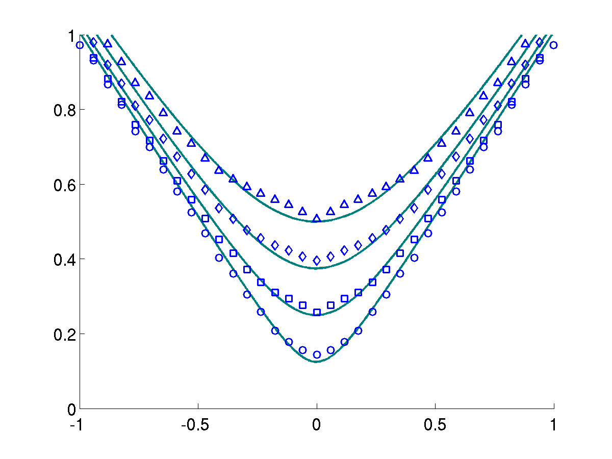
Fig. 6: Distance estimates (markers) for $d(x(y,s),(z_{i},0))$ for $y=(0,0)$ and $s=.125,.25,.375,.5$, plotted along with the true distances (solid curves).

5.4 Discussion of sources of numerical errors and instability

Examining Figure 6, one can see that in each of the estimated distance curves, the distances are over-estimated for $z=(z_{i},0)$ near $y=(0,0)$. This error results in part from the distance estimation method. For example, when $z=y$ the correct distance $d=r+s$ would be obtained by taking $r=0$. On the other hand, when $z=y$, both of the wave caps used in the distance estimation procedure are centered on the same point, so for $0\leq r\leq h$ the variable wave cap, $\operatorname{cap}_{\Gamma}(z,s,r)$, coincides with $\operatorname{cap}_{\Gamma}(z,s,r)\cap\operatorname{cap}_{\Gamma}(y,s,h)$. From the definition of $r_{h}$, we find that we will have $0<r_{h}<h$. Thus the distance estimate $d_{h}$ will necessarily over-estimate $d(y,x(y,s))$. Similar remarks apply for estimating $d((z_{i},0),x(y,s))$ for $(z_{i},0)$ near $y$, although the strength of this effect decreases as $(z_{i},0)$ gets further from $y$. We call this source of error geometric distortion, since it results entirely from the geometry of our distance estimation procedure and is independent of errors arising from the control problems. In Figure 7 we depict the geometric distortion by repeating our distance estimation technique with exact volume measurements. Note that the distances in Figure 7 are overestimated at all points, which contrasts most with the distances estimated at large offsets in Figure 6.

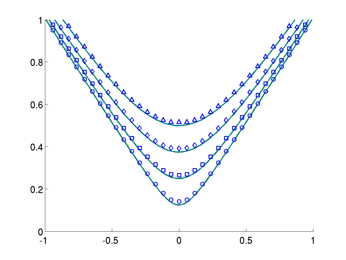
Fig. 7: Demonstration of geometric distortion. Distances (markers) are estimated by using the distance estimation technique on exact volumes and plotted for $d(x(y,s),(z_{i},0))$ for $y=(0,0)$ and $s=.125,.25,.375,.5$, along with the true distances (solid curves).

Our numerical tests suggest that the dominant source of error comes from the control step. In order to discuss this instability, we return to considering the continuum problem. Taking $\tau\in C(\overline{\Gamma})$, we can ask whether there exists $f\in H^{s}(S_{\tau})$ for some $s\in\mathbb{R}$ for which $W_{\tau}f=1_{M(\tau)}$. This question can be answered by considering the more general problem of exact controllability, in which one seeks to determine when the equation $(u^{f}(T,\cdot),\partial_{t}u^{f}(T,\cdot))=(w_{0},w_{1})$ has a solution in $H^{s}(S_{\tau})$ for any $(w_{0},w_{1})$ belonging to an appropriate space of Cauchy data for the wave equation.

In [4], the question of exact controllability is considered. One of the main results of that paper is that the ray geometry of the wave equation can be used to determine necessary and sufficient conditions for exact controllability. Using the same set of ideas to those in [4], it is shown in [3] that in order for exact controllability to hold for $W_{\tau}$ in $M(\tau)$ from $S_{\tau}$, the following geometric controllability condition must hold:

Each generalized bicharacteristic $(x(t),t)$ satisfying $x(T)\in M(\tau)$, passes over $S_{\tau}\cup S_{\tau}^{\prime}$ in a non-diffractive point.

Here, $S_{\tau}^{\prime}=\{(t,x)\in\Gamma\times(T,2T):T\leq t\leq T+\tau(x)\}$. We recall that $S_{\tau}$ is defined by (3), and note that $S_{\tau}^{\prime}$ is the temporal reflection of $S_{\tau}$ across $t=T$. For a generalized bicharacteristic $(x(t),t)$, the path $x(t)$ is a unit speed geodesic in the interior of M and it is reflected according to Snell’s law when it intersects the boundary $\partial M$ transversally. Tangential intersections with the boundary can cause the path to glide along the boundary, and in the case of an infinite-order contact, the path $x(t)$ can be continued in many ways, see [4]. We refer also to [4] for the definition of non-diffractive points. The geometric controllability condition is necessary for exact control to hold from $S_{\tau}$, since when it fails for $(x,\xi)\in S^{*}(M(\tau))$, propagation of singularities implies that for any $s\in\mathbb{R}$ and any $f\in H^{s}(S_{\tau})$, $(x,\xi)\not\in\operatorname{WF}(u^{f}(T,\cdot))$, see e.g. [15, Section 23]. Here, $\operatorname{WF}(u^{f}(T,\cdot))$ denotes the wave front set of $u^{f}(T,\cdot)$, and we refer to [16, Def. 8.1.2] for its definition. We have also provided the definition of wave front set in Appendix A. Thus, if $w\in L^{2}(M(\tau))$ has $(x,\xi)\in\operatorname{WF}(w)$ then, for each $s\in\mathbb{R}$, there does not exist $f\in H^{s}(S_{\tau})$ for which $W_{\tau}f=w$.

In our computational experiment, the geometric controllability condition actually fails over every point in $M(\tau)$. This is due to the fact that at each $x\in M(\tau)$ there exists a family of unit-speed geodesic rays with $(\gamma(T),\dot{\gamma}(T))=(x,\xi)\in S_{x}(M)$ and $\xi$ belonging to a cone over $x$, for which the corresponding geodesics $\gamma$ fail to pass over $S_{\tau}\cup S_{\tau}^{\prime}$. In our computational experiment, we observe instabilities near those $x\in M(\tau)$ where $\operatorname{WF}(1_{M(\tau)})$ meets the cone over which exact control fails. In the case of $\tau=\tau_{y}^{s+h}\vee s1_{\Gamma}$, these effects occur where $\partial M(\tau)$ fails to be $C^{\infty}$ smooth and $\{x\}\times(\mathbb{R}^{n}\setminus 0)\subset\operatorname{WF}(1_{M(\tau)})$ . We refer to Appendix A for further analysis. In particular these effects occur for $x$ in the bottom left and right edges of $\operatorname{cap}_{\Gamma}(y,s,h)$, where $\partial M(\tau)$ fails even to be $C^{1}$. In addition, we similarly observe instabilities near the points $(\pm L,-s)$, where the flat portion of $\partial M(\tau)$ transitions into a circle and fails to be $C^{2}$.

We demonstrate these effects in Figure 8, by plotting a wavefield $u^{f}(T,\cdot)$ approximating $1_{M(\tau)}$ for $y=(0,0),s=.5$, and $h=.2$. The former instabilities occur near the points $(\pm.5,-.5)$, and the latter instabilities occur near $(\pm 1.15,-.5)$. We contrast this with the case where $\tau=\tau_{y}^{s+h}$, which we show in Figure 8. In this second example, the domain of influence is a disk and every co-vector in $\operatorname{WF}(1_{M(\tau)})$ can be controlled, and unlike the first example, we observe no instabilities. Note that in all of the examples in Figure 8 we use a smaller $\Gamma$ than in our distance calculations, using $L=1.153$ and a finer basis with $a_{t}=a_{x}=16\cdot 10^{3}$.

[figure]subcapbesideposition=center

[]

[]

[]

[]

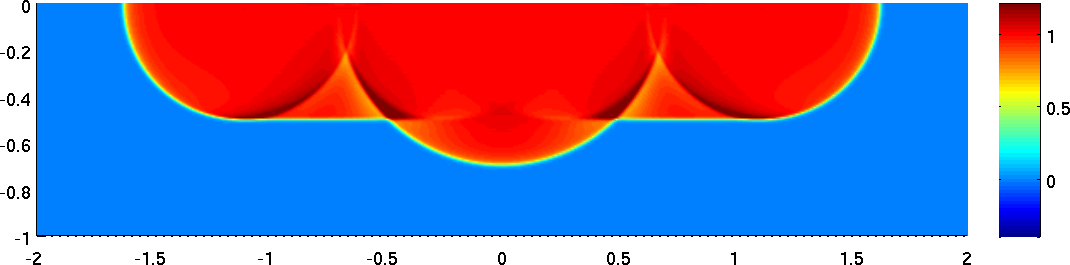
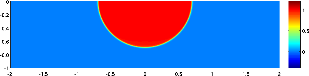
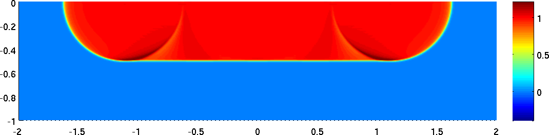
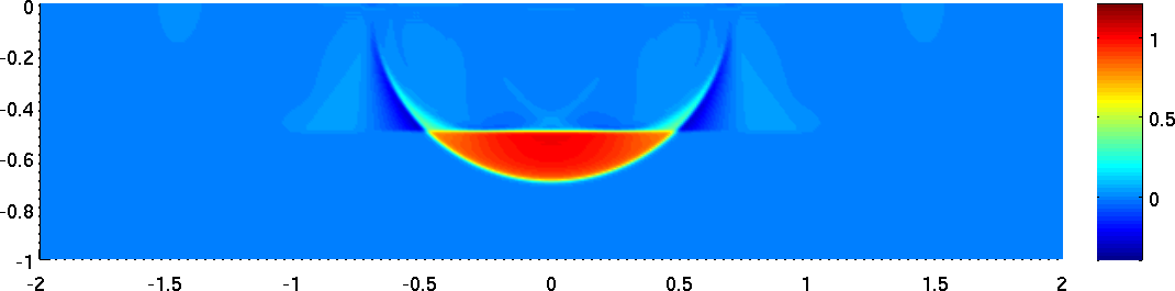
Fig. 8: (a) wavefield demonstrating instability of the solution to the control problem when $\operatorname{WF}(1_{M(\tau)})$ contains uncontrollable directions over $(\pm.5,-.5)$ and $(\pm 1.15,-.5)$ (b) A wavefield for which all directions in $\operatorname{WF}(1_{M(\tau)})$ are controlled. (c) Another wavefield demonstrating instability, with uncontrollable directions in $\operatorname{WF}(1_{M(\tau)})$ over $(\pm 1.15,-.5)$. (d) The difference between the wavefields in (a) and (c), note that this corresponds to an approximation to $1_{M(\operatorname{cap}(y,s,h))}$ as used in the distance estimation procedure. Moreover, the instabilities in (a) and (c) located over $(\pm 1.15,-.5)$ cancel each other.

In Figure 8 we plot the wavefield $u^{f}(T,\cdot)$ that approximates $1_{M(s1_{\Gamma})}$. Note that as in the case of $\tau=\tau_{y}^{s+h}\vee s1_{\Gamma}$, we observe instabilities near the points $(\pm 1.15,-.5)$. In Figure 8 we plot the difference between the wave fields approximating $1_{M(\tau_{y}^{s+h}\vee s1_{\Gamma})}$ and $1_{M(s1_{\Gamma})}$, and note that this difference yields an approximation to the characteristic function of $\operatorname{cap}_{\Gamma}(y,s,h)$. In particular, notice that the instabilities observed near $(\pm 1.15,-.5)$ in Figures 8 and 8 completely cancel in Figure 8. Since our distance determination relies primarily on the volumes of wave caps, which are obtained by taking differences in this fashion, we find that the instabilities near the cap bases tend to provide the main source of error for our distance estimation procedure.

6 Conclusions

In this paper we have demonstrated a method to construct distances between boundary points and interior points with fixed semi-geodesic coordinates. The procedure is local in that it utilizes the local Neumann-to-Dirichlet map for an acoustic wave equation on a Riemannian manifold with boundary. Our procedure differs from earlier results in that it utilizes volume computations derived from local data in order to construct distances. Finally, we have provided a computational experiment to demonstrate the implementation of our distance determination procedure and we have discussed the main sources of numerical error.

Appendix A Wave front set of $1_{M(\tau)}$

In Section 5 all of the functions $\tau$ that we consider give rise to sets $M(\tau)$ with piecewise smooth boundary. For all such $\tau$, if $x\in\partial M(\tau)$ is a point for which $\partial M(\tau)$ is not smooth at $x$, then either $\partial M(\tau)$ is not $C^{1}$ at $x$, or $\partial M(\tau)$ fails to be $C^{2}$ at $x$. In this section, we examine the former case, by computing the wave front set of $1_{M(\tau)}$ over a point $x$ where $\partial M(\tau)$ fails to be $C^{1}$. The other case is similar and we omit it. In particular, we will show the following lemma:

Lemma 10.

Let $h:\mathbb{R}\to\mathbb{R}$ be continuous, and suppose that $h$ is smooth on $(-\infty,0)$ and on $(0,\infty)$, and that $h$ does not belong to $C^{1}(\mathbb{R})$. Let $A$ be the set, $A=\{(x^{1},x^{2})\in\mathbb{R}^{2}:\ x^{2}\leq h(x^{1})\}.$ Then, $\{0\}\times(\mathbb{R}^{2}\setminus 0)\subset\operatorname{WF}(1_{A})$.

From the lemma, it follows that if $\tau$ is one of the functions considered in Section 5 and $\partial M(\tau)$ fails to be $C^{1}$ at $x\in\partial M(\tau)$, then $\{x\}\times(\mathbb{R}^{2}\setminus 0)\subset\operatorname{WF}(1_{M(\tau)})$. Put differently, $\operatorname{WF}(1_{M(\tau)})$ contains all cotangent directions above the point $x$.

Before proceeding with the proof, we recall the definition of wave front set,

Definition 11.

Let $X\subset R^{n}$ open. If $u\in\mathcal{D}^{\prime}(X)$, then the closed subset of $X\times(\mathbb{R}^{n}\setminus 0)$ defined by,

$$\operatorname{WF}(u)=\{(x,\xi)\in X\times(\mathbb{R}^{n}\setminus 0):\xi\in\Sigma_{x}(u)\}$$

is called the wave front set of $u$, where $\Sigma_{x}(u)$ is the set

$$\Sigma_{x}(u)=\bigcap_{\phi}\Sigma(\phi u),\quad\phi\in C_{0}^{\infty}(X),~{}\phi(x)\neq 0,$$

and, for $v\in\mathcal{D}^{\prime}(X)$, $\Sigma(v)$ is the complement of the set of $\eta$ in $\mathbb{R}^{n}\setminus 0$ for which there exists a conic neighborhood $V$ of $\eta$ such that for each $N\in\mathbb{N}$ there exist $C_{N}>0$ such that, for all $\xi\in V$,

$$|\hat{v}(\xi)|\leq C_{N}(1+|\xi|)^{-N}.$$

To prove Lemma 10, we require the following result,

Lemma 12.

Let $h\in\mathbb{R}$, $u\in C_{0}^{\infty}(\mathbb{R})$. Suppose that $\phi\in C^{\infty}(\mathbb{R})$ is real valued and has no critical points in $\mathop{\operator@font supp}\nolimits(u)$. Then

$$\int_{-\infty}^{h}u(x)e^{-i\lambda\phi(x)}dx=\frac{iu(h)e^{-i\lambda\phi(h)}}{\lambda\phi^{\prime}(h)}+\frac{\left.\partial_{x}(u/\phi^{\prime})\right|_{x=h}e^{-i\lambda\phi(h)}}{\lambda^{2}\phi^{\prime}(h)}+\frac{R(\lambda,h,\phi,u)}{\lambda^{3}},$$

where $|R|$ is bounded by a constant that depends only on $\mathop{\operator@font supp}\nolimits(u)$, $\min_{x\in\mathop{\operator@font supp}\nolimits(u)}|\phi^{\prime}(x)|$ and the $C^{3}$ norms of $u$ and $\phi$.

Proof. We define the differential operator $L=i\phi^{\prime-1}\partial_{x}$. Then

$$\int_{-\infty}^{h}ue^{-i\lambda\phi}dx=\frac{1}{\lambda}\int_{-\infty}^{h}uLe^{-i\lambda\phi}dx$$

$$\quad=\left.\frac{iue^{-i\lambda\phi}}{\lambda\phi^{\prime}}\right|_{x=h}+\frac{1}{\lambda}\int_{-\infty}^{h}(L^{*}u)e^{-i\lambda\phi}dx.$$

Notice, $L^{*}u=-i\partial_{x}(u/\phi^{\prime})$. Then,

$$\frac{1}{\lambda}\int_{-\infty}^{h}(L^{*}u)e^{-i\lambda\phi}dx=\frac{1}{\lambda^{2}}\int_{-\infty}^{h}(L^{*}u)Le^{-i\lambda\phi}dx$$

$$\quad=\left.\frac{\partial_{x}(u/\phi^{\prime})e^{-i\lambda\phi}}{\lambda^{2}\phi^{\prime}}\right|_{x=h}+\frac{1}{\lambda^{2}}\int_{-\infty}^{h}((L^{*})^{2}u)e^{-i\lambda\phi}dx.$$

Finally,

$$\frac{1}{\lambda^{2}}\int_{-\infty}^{h}((L^{*})^{2}u)e^{-i\lambda\phi}dx=\frac{1}{\lambda^{3}}\int_{-\infty}^{h}((L^{*})^{2}u)Le^{-i\lambda\phi}dx$$

$$\quad=\left.\frac{i((L^{*})^{2}u)e^{-i\lambda\phi}}{\lambda^{3}\phi^{\prime}}\right|_{x=h}+\frac{1}{\lambda^{3}}\int_{-\infty}^{h}((L^{*})^{3}u)e^{-i\lambda\phi}dx.\qquad\end@proof$$

of Lemma 10.

Let $u\in C_{0}^{\infty}(\mathbb{R}^{2})$ and suppose that $u=1$ near the origin. We consider the Fourier transform

$$\widehat{u1_{A}}(\lambda\xi) =\int_{\mathbb{R}^{2}}u(x)1_{A}(x)e^{-i\lambda\xi x}dx$$

$$=\int_{-\infty}^{+\infty}e^{-i\lambda\xi_{1}x^{1}}\int_{-\infty}^{h(x^{1})}u(x)e^{-i\lambda\xi_{2}x^{2}}dx^{2}dx^{1},$$

where $\xi$ is a unit vector and $\lambda>0$.

Suppose first that $\xi_{2}\neq 0$. Then

$$\int_{-\infty}^{h(x^{1})}u(x)e^{-i\lambda\xi_{2}x^{2}}dx^{2}=\frac{iw(x^{1})e^{-i\lambda\xi_{2}h(x^{1})}}{\lambda\xi_{2}}+\frac{v(x^{1})e^{-i\lambda\xi_{2}h(x^{1})}}{\lambda^{2}\xi_{2}^{2}}+\frac{R}{\lambda^{3}},$$

where $w(x^{1})=u(x^{1},h(x^{1}))$ and $v(x^{1})=\partial_{x^{2}}u(x^{1},h(x^{1}))$. Note that $R$ is compactly supported with respect to $x^{1}$ since $u$ is. Note also that $w$ and $v$ are compactly supported and $w=1$ near the origin. If $\mathop{\operator@font supp}\nolimits(u)$ is small then $\mathop{\operator@font supp}\nolimits(w)$ and $\mathop{\operator@font supp}\nolimits(v)$ are also small. Moreover, if $\mathop{\operator@font supp}\nolimits(w)\cup\mathop{\operator@font supp}\nolimits(v)$ is small enough then $h$ is smooth in $(\mathop{\operator@font supp}\nolimits(w)\cup\mathop{\operator@font supp}\nolimits(v))\setminus 0$. In particular, $w$ and $v$ are smooth then.

We define $\phi(x^{1})=\xi_{1}x^{1}+\xi_{2}h(x^{1})$, $\phi_{\pm}=\phi|_{\pm x^{1}>0}$, and define also $h_{\pm}$ analogously. Suppose that $\phi_{-}^{\prime}(0)=\xi_{1}+h_{-}^{\prime}(0)\xi_{2}\neq 0$. Then $\phi$ has no critical points in the set $\{x^{1}<0\}\cap\mathop{\operator@font supp}\nolimits(w)$ if $\mathop{\operator@font supp}\nolimits(w)$ is small enough. Therefore

$$\int_{-\infty}^{0}we^{-i\lambda\phi}dx^{1}=\frac{i}{\lambda\phi_{-}^{\prime}(0)}+\frac{R_{+}(\lambda,h,\phi,u)}{\lambda^{2}}.$$

Likewise, if also $\phi_{+}^{\prime}(0)\neq 0$, then

$$\int_{0}^{+\infty}we^{-i\lambda\phi}dx^{1}=\frac{-i}{\lambda\phi_{+}^{\prime}(0)}+\frac{R_{-}(\lambda,h,\phi,u)}{\lambda^{2}}.$$

So,

$$\int_{-\infty}^{+\infty}we^{-i\lambda\phi}dx^{1}=i\left(\frac{1}{\phi_{-}^{\prime}(0)}-\frac{1}{\phi_{+}^{\prime}(0)}\right)\lambda^{-1}+\mathcal{O}(\lambda^{-2}).$$

An analogous argument applies to $v$, showing that,

$$\int_{-\infty}^{+\infty}ve^{-i\lambda\phi}dx^{1}=\mathcal{O}(\lambda^{-1}).$$

Hence, we conclude,

$$\widehat{u1_{A}}(\lambda\xi)=\frac{1}{\xi_{2}}\left(\frac{1}{\phi_{+}^{\prime}(0)}-\frac{1}{\phi_{-}^{\prime}(0)}\right)\lambda^{-2}+\mathcal{O}(\lambda^{-3}).$$

Thus $\widehat{u1_{A}}$ does not decay rapidly if $\phi_{+}^{\prime}(0)\neq\phi_{-}^{\prime}(0)$ which again is equivalent to $h_{+}^{\prime}(0)\neq h_{-}^{\prime}(0)$.

To summarize, if $h_{+}^{\prime}(0)\neq h_{-}^{\prime}(0)$ then all the directions except possibly $(1,0)$ and the four directions

$$(-h_{\pm}^{\prime}(0)\xi^{2},\xi^{2}),\quad\text{where}\quad|\xi_{2}|=(|h_{\pm}^{\prime}(0)|^{2}+1)^{-1/2},$$

are in $\Sigma_{0}(1_{A})$. Finally, since $\Sigma_{0}(1_{A})$, is a closed conic subset of $\mathbb{R}^{2}\setminus 0$, we conclude that $\Sigma_{0}(1_{A})=\mathbb{R}^{2}\setminus 0$, and hence $\{0\}\times(\mathbb{R}^{2}\setminus 0)\subset\operatorname{WF}(1_{A})$.   ∎

References

- [1] G. Alessandrini, Stable determination of conductivity by boundary measurements, Appl. Anal., 27 (1988), pp. 153–172.
- [2] R. Alexander and S. Alexander, Geodesics in riemannian manifolds-with-boundary, Indiana University Math Journal, 30 (1981), pp. 481–488.
- [3] C. Bardos and M. Belishev, The wave shaping problem, in Partial Differential Equations and Functional Analysis, J. Cea, D. Chenais, G. Geymonat, and J. Lions, eds., vol. 22 of Progress in Nonlinear Differential Equations and Their Applications, Birkhäuser Boston, 1996, pp. 41–59.
- [4] C. Bardos, G. Lebeau, and J. Rauch, Sharp sufficient conditions for the observation, control, and stabilization of waves from the boundary, SIAM J. Control Optim., 30 (1992), pp. 1024–1065.
- [5] M. Belishev and Y. Y. Gotlib, Dynamical variant of the BC-method: theory and numerical testing., Journal of Inverse & Ill-Posed Problems, 7 (1999), p. 221.
- [6] M. I. Belishev, An approach to multidimensional inverse problems for the wave equation, Dokl. Akad. Nauk SSSR, 297 (1987), pp. 524–527.
- [7] , Boundary control in reconstruction of manifolds and metrics (the BC method), Inverse Problems, 13 (1997), pp. R1–R45.
- [8] M. I. Belishev and Y. V. Kurylev, To the reconstruction of a Riemannian manifold via its spectral data (BC-method), Comm. Partial Differential Equations, 17 (1992), pp. 767–804.
- [9] M. Bellassoued and D. Dos Santos Ferreira, Stability estimates for the anisotropic wave equation from the Dirichlet-to-Neumann map, Inverse Probl. Imaging, 5 (2011), pp. 745–773.
- [10] K. Bingham, Y. Kurylev, M. Lassas, and S. Siltanen, Iterative time-reversal control for inverse problems, Inverse Probl. Imaging, 2 (2008), pp. 63–81.
- [11] A. S. Blagoveshchenskii, The local method of solution of the nonstationary inverse problem for an inhomogeneous string, Trudy Mat. Inst. Steklov., 115 (1971), p. 28–38.
- [12] A.-P. Calderón, On an inverse boundary value problem, in Seminar on Numerical Analysis and its Applications to Continuum Physics, Soc. Brasil. Mat., Rio de Janeiro, 1980, pp. 65–73.
- [13] M. Dahl, A. Kirpichnikova, and M. Lassas, Focusing waves in unknown media by modified time reversal iteration, SIAM Journal on Control and Optimization, 48 (2009), pp. 839–858.
- [14] M. de Hoop, S. Holman, E. Iversen, M. Lassas, and B. Ursin, Reconstruction of a conformally Euclidean metric from local boundary diffraction travel times, SIAM Journal on Mathematical Analysis, 46 (2014), pp. 3705–3726.
- [15] L. Hörmander, The analysis of linear partial differential operators. III, vol. 274 of Grundlehren der Mathematischen Wissenschaften, Springer-Verlag, Berlin, 1985.
- [16] , The analysis of linear partial differential operators. I, vol. 256 of Grundlehren der Mathematischen Wissenschaften, Springer-Verlag, Berlin, 1990.
- [17] P. Hubral and T. Krey, Interval Velocities from Seismic Reflection Time Measurements, Society of Exploration Geophysicists, 1980.
- [18] S. I. Kabanikhin, A. D. Satybaev, and M. A. Shishlenin, Direct methods of solving multidimensional inverse hyperbolic problems, Inverse and Ill-posed Problems Series, VSP, Utrecht, 2005.
- [19] A. Katchalov, Y. Kurylev, and M. Lassas, Inverse boundary spectral problems, vol. 123 of Monographs and Surveys in Pure and Applied Mathematics, Chapman & Hall/CRC, Boca Raton, FL, 2001.
- [20] A. Katsuda, Y. Kurylev, and M. Lassas, Stability of boundary distance representation and reconstruction of Riemannian manifolds, Inverse Problems and Imaging, 1 (2007), pp. 135–157.
- [21] A. Kirsch, An Introduction to the Mathematical Theory of Inverse Problems, Springer, New York, 2011.
- [22] I. Lasiecka and R. Triggiani, Sharp regularity theory for second order hyperbolic equations of Neumann type. part 1. nonhomogeneous data, Annali di Mathematica Pura ed Applicata, 157 (1990).
- [23] M. Lassas and L. Oksanen, Inverse problem for the Riemannian wave equation with Dirichlet data and Neumann data on disjoint sets, Duke Math. J., 163 (2014), pp. 1071–1103.
- [24] S. Liu and L. Oksanen, A Lipschitz stable reconstruction formula for the inverse problem for the wave equation, Trans. Amer. Math. Soc. (to appear). Preprint arXiv:1210.1094, (2012).
- [25] A. Logg, K.-A. Mardal, G. N. Wells, et al., Automated Solution of Differential Equations by the Finite Element Method, Springer, 2012.
- [26] N. Mandache, Exponential instability in an inverse problem for the Schrödinger equation, Inverse Problems, 17 (2001), pp. 1435–1444.
- [27] C. Montalto, Stable determination of a simple metric, a covector field and a potential from the hyperbolic dirichlet-to-neumann map, Communications in Partial Differential Equations, 39 (2014), pp. 120–145.
- [28] L. Oksanen, Solving an inverse problem for the wave equation by using a minimization algorithm and time-reversed measurements, Inverse Problems and Imaging, 5 (2011), pp. 731–744.
- [29] L. Oksanen, Inverse obstacle problem for the non-stationary wave equation with an unknown background, Communications in Partial Differential Equations, 38 (2013), pp. 1492–1518.
- [30] , Solving an inverse obstacle problem for the wave equation by using the boundary control method, Inverse Problems, 29 (2013), pp. 035004, 12.
- [31] L. Pestov, V. Bolgova, and O. Kazarina, Numerical recovering of a density by the BC-method, Inverse Probl. Imaging, 4 (2010), pp. 703–712.
- [32] P. Stefanov and G. Uhlmann, Stability estimates for the hyperbolic Dirichlet to Neumann map in anisotropic media, Journal of Functional Analysis, 154 (1998), pp. 330 – 358.
- [33] P. Stefanov and G. Uhlmann, Stable determination of generic simple metrics from the hyperbolic Dirichlet-to-Neumann map, Int. Math. Res. Not., (2005), pp. 1047–1061.
- [34] J. Sylvester and G. Uhlmann, A global uniqueness theorem for an inverse boundary value problem, Ann. of Math. (2), 125 (1987), pp. 153–169.
- [35] D. Tataru, Unique continuation for solutions to pde’s; between Hörmander’s theorem and Holmgren’s theorem, Communications in Partial Differential Equations, 20 (1995), pp. 855–884.
- [36] D. Tataru, On the regularity of boundary traces for the wave equation, Ann. Scuola Norm. Sup. Pisa Cl. Sci. (4), 26 (1998), pp. 185–206.
- [37] K. Wapenaar, J. Thorbecke, J. van der Neut, F. Broggini, E. Slob, and R. Snieder, Marchenko imaging, GEOPHYSICS, 79 (2014), pp. WA39–WA57.