Visualization and analysis of the Kohn-Sham kinetic energy density and its orbital-free description in molecules

Abstract

We visualize the Kohn-Sham kinetic energy density (KED), and the ingredients – the electron density, its gradient and Laplacian – used to construct orbital-free models of it, for the AE6 test set of molecules. These are compared to related quantities used in metaGGA’s, to characterize two important limits – the gradient expansion and the localized-electron limit typified by the covalent bond. We find the second-order gradient expansion of the KED to be a surprisingly successful predictor of the exact KED, particularly at low densities where this approximation fails for exchange. This contradicts the conjointness conjecture that the optimal enhancement factors for orbital-free kinetic and exchange energy functionals are closely similar in form. In addition we find significant problems with a recent metaGGA-level orbital-free KED, especially for regions of strong electron localization. We define an orbital-free description of electron localization and a revised metaGGA that improves upon atomization energies significantly.

I Introduction

The Kohn-Sham kinetic energy density (KED) – the kinetic energy per volume defined by the orbitals generated by the Kohn-Sham equation – plays a central role in the development of density functional theory (DFT). In the “Jacob’s Ladder” paradigm for characterizing the exchange-correlation (XC) energy in density functional theory, Perdew and Schmidt (2001) the KED is the key variable of the central, metaGGA rung of functionals. Becke (1998); Perdew et al. (1999); Tao et al. (2003); Zhao and Truhlar (2006) As a local energy density, it provides information about electronic structure complementary to that provided by the local electron density and its derivatives that describe lower rungs of DFT. Particularly important is its ability to distinguish between regions of electron localization,Becke and Edgecombe (1990); Sun et al. (2013); Hao, Armiento, and Mattsson (2014) for which self-interaction error is important, and regions of delocalization such as metals where they are not.

The centrality of the KED in DFT development is highlighted by the implicit role it plays in the rungs of DFT lower than the metaGGA. These may be thought of as a Jacob’s ladder of approximations to the KED as much as one of approximations to the exchange-correlation energy. The lowest rung of the XC ladder, the local density approximation or LDA, Kohn and Sham (1965) corresponds to the Thomas-Fermi approximation Thomas (1927); Fermi (1928) to the KED. The more commonly used generalized gradient approximation (GGA) introduces, in addition to the local density, the gradient of the density as a variable in XC functional construction. The same information is contained in the von Weizsäcker KED Weizsäcker (1935) that describes the KE of localized electron pairs. It has been used to generate a large number of GGA’s for the KED, both empirical Karasiev et al. (2009); Tran and Wesolowski (2002); Lacks and Gordon (1994); Thakkar (1992) and nonempirical, Constantin et al. (2011); Karasiev et al. (2013) though not with the success they have enjoyed in describing the XC energy. To describe the XC energy at the next, metaGGA, level of the theory, not only the KED, but also the Laplacian of the density Jemmer and Knowles (1995); Cancio, Wagner, and Wood (2012); Pittalis and Räsänen (2009, 2010) may be used as an additional variable in functional construction. A metaGGA description of the KED is thus possible, using the Laplacian.Perdew and Constantin (2007); Karasiev et al. (2009); Laricchia et al. (2014) The similarity of the KED and XC functional ladders leads to a conjointness conjectureLee, Lee, and Parr (1991) that the optimal orbital-free correction to the Thomas-Fermi KE is similar in form to that for LDA exchange. More importantly, it enables one to apply lessons learned in constructing the one functional to constructing the other. This is important for orbital-free DFT, in which the Kohn-Sham KED is replaced by an explicit functional of the density, removing completely the need for orbitals.

The orbital-free modeling of the KED has taken on increasing importance in recent years. Karasiev, D.Chakraborty, and Trickey (2013); Akimov and Prezhdo (2015) Given a cubic scaling in the number orbitals, the Kohn-Sham method becomes prohibitively expensive for large-scale applications that require the accuracy of atomistic simulation. These involve applications such as the dynamics of nanoscale materials Akimov and Prezhdo (2015) requiring intrinsically large system size, high throughput as in alloy design, or a need for large number of excited states, as can occur for finite-temperature applications such as warm dense matter (WDM). Graziani (2014); Karasiev et al. (2014) A completely orbital-free density functional theory (OFDFT), using an orbital-free expression for the kinetic energy, becomes an important tool in these cases. Unfortunately, OFDFT is inherently less accurate than Kohn-Sham DFT; for example, the Thomas-Fermi approximation is unable to predict molecular binding, Teller (1962) something the LDA has no problem doing. Nevertheless, nonlocal models Wang, Govind, and Carter (1999, 2001); Huang and Carter (2010); Ke et al. (2014) have achieved reasonably high accuracy, allowing for impressive calculations for solid-state applications, Hung and Carter (2011); Shin and Carter (2013) albeit within the limitation of requiring different functionals for different material classes. And, with a focus on improving potentials and thus forces in the context of WDM, a number of GGA-level OFDFT’s have been developed in recent years. Karasiev et al. (2009, 2013); Karasiev, D.Chakraborty, and Trickey (2013) These coincide with improvements in infrastructure for practical calculations. Karasiev and Trickey (2012); Hung et al. (2010)

A third role of the KED has been as a tool for visualizing the electronic structure of the chemical bond. The kinetic energy density has been the subject of investigation Ruedenberg and Schmidt (2009); Tachibana (2001) particularly as a localized-orbital locator (LOL), Schmider and Becke (2000); Jacobsen (2013) and an impressive number of related quantities have been defined and investigated as well. Anderson, Ayers, and Hernandez (2010) Perhaps the most popular is the electron localization factor ELF, which is based upon a comparison of the Kohn-Sham to Thomas-Fermi and von Weizsäcker KED’s. Becke and Edgecombe (1990); Silvi and Savin (1994); Burnus, Marques, and Gross (2005) It is of particular importance for the development of metaGGA’s for the XC energy and in the conceptual understanding of why they work. Hao, Armiento, and Mattsson (2014); Sun et al. (2013) Also of note is the quantum theory of atoms in molecules (QTAIM),Bader (1990, 1991); Matta, Massa, and Keith (2011) an approach to visualization which is in some ways an orbital-free version of ELF analysis, using gradients and Laplacians of the density to analyze bonding structures.

Despite the strong connection between the arguments used to build XC metaGGA’s Becke (1998); Tao et al. (2003); Perdew et al. (2009); Sun et al. (2013) and those used to visualize the chemical bond, the tool of visualization has not often been used to provide feedback into DFT development. The properties of the exchange-correlation hole, describing the hole around an electron caused by Pauli exclusion and Coulomb repulsion have been an important tool in the construction of both GGA’s and their successors. Perdew, Burke, and Wang (1996); Becke (1983); Burke et al. (2014) In particular, the visualization of the hole has been a valuable tool in assessing the accuracy of DFT’s. Hood et al. (1997); Cancio and Fong (2012) However, the exchange-correlation hole is a difficult many-body calculation, and the dependence of measurables like the atomization energy or bond length on the nature of the XC hole occurs implicitly through the mediation of complex functionals and thus is hard to determine. (But connections can sometimes be made. Cancio, Chou, and Hood (2001); Cancio and Chou (2006)) In the case of the KED, however, visualization is of direct help Xia and Carter (2015a); Trickey, Karasiev, and Chakraborty (2015); Xia and Carter (2015b) – how an orbital-free density functional theory for the Kohn-Sham KED actually compares to the real thing requires no more than running a standard DFT code and visualizing the results.

In this paper, we perform highly converged Kohn-Sham DFT calculations and visualize the electron density, its gradient and Laplacian, the KED and some approximations for these used in DFT, for the AE6 test set of molecules, in a pseudopotential plane wave approach.

The AE6 test set Lynch and Truhlar (2003) is a set of 6 molecules – Cyclobutane ($\mathrm{C_{4}H_{8}}$), Propyne ($\mathrm{C_{3}H_{4}}$), Glyoxal ($\mathrm{C_{2}H_{2}O_{2}}$), Silicon Monoxide (SiO), Disulfur (S₂), and Silicon Tetrahydride ($\mathrm{SiH_{4}}$) – chosen for their ability to reproduce the average atomization energy of common DFT’s over much larger test sets. For such a small set the AE6 shows a richness of bonding scenarios – single, double, and triple bonds, covalent to nearly ionic, including first and second row atoms, and a large-cation, small-anion system similar to important semiconductors like GaN. Thus it covers many situations commonly seen in organic chemistry and in semiconductors as well.

Our motive for using pseudopotentials is two-fold. First of all, many current OFDFT applications rely upon the use of pseudopotentials, Huang and Carter (2010); Ke et al. (2014) although more accurate approaches do exist. Lehtomäki et al. (2014) More importantly, the pseudopotential plane-wave approach permits an arbitrary convergence of the particle density associated with the pseudopotential and thus a map between a $v-$representable density and the related KE density that is as accurate as possible. It thus gives insight into the universal map between kinetic energy and density that is a corollary of the Hohenberg-Kohn theorem. Although the method does not produce the correct density for real molecules, and thus introduces errors into the chemical characterization of the test set, it arguably gives us simpler problem to model, and much of what is learned for pseudopotential systems should help to construct functionals for the all-electron case. KT (1) The use of pseudopotentials enables particularly the study of asymptotic features not possible with a typical gaussian basis set.

Finally, the choice of exchange-correlation functional is irrelevant to the universal mapping between the Kohn-Sham kinetic energy and the charge density, in which the electrostatic potential energy plays no role. We work with the LDA and PBE exchange-correlation functionals, which produce reasonably accurate bond lengths for the test set and should produce densities and orbitals close to the exact ones for pseudopotential systems.

In our visualization, we have deemphasized (but do not ignore) the ELF, already studied extensively for a large number of molecular systems. We look rather at the basic ingredients of the orbital-free KED, the electron density $n$, and related derivatives $\left|\nabla n\right|^{2}/n$ and $\nabla^{2}n$, focusing especially on applications of their use in DFT. One is a common approximation based upon the gradient expansion in the limit of slowly varying densities used in many metaGGA’s to replace $\nabla^{2}n$, a natural descriptor in this limit, for $\tau_{KS}$. The second is a sophisticated metaGGA-level orbital-free model of the Kohn-Sham KED, the mGGA. Perdew and Constantin (2007) This takes advantage of lessons learned in developing metaGGA’s for exchange, particularly of defining and respecting key constraints and limiting cases for the kinetic energy. Despite the promise of its design philosophy, the mGGA has deficiencies – its potential does not bind molecules Karasiev et al. (2009) and even used non-self-consistently fails to improve upon Thomas-Fermi predictions of atomization energies.Laricchia et al. (2014) However, it is of value as a starting point of thinking how to construct a metaGGA; and since it is a model of the kinetic energy density as such, it is directly testable by visualization of this quantity. Our investigation of the mGGA shows, despite its excellent description of atomic KED’s, surprising failures in its description of the KED of bonds, and thus in its prediction of atomization energies. Our visualization work makes it easy to diagnose and suggest a fix to this problem, one which defines, and demonstrates at least in an ad hoc fashion, a potential lower bound to the KED.

The rest of this paper is organized as follows: Sec. II describes the theoretical background of the paper – the density functional theory of the kinetic energy and its relation to exchange in metaGGA’s. Sec. III covers the basic methodology used. Sec. IV details the chief results of visualization, while Sec. V applies the lessons learned to construct and make preliminary tests of a correction to the Perdew-Constantin mGGA and Sec. VI presents our conclusions.

II Theory

The positive definite form of the kinetic energy density in Kohn-Sham theory is given by

$$\tau_{KS}=\frac{1}{2}\sum_{i}^{occup}f_{i}\left|\nabla\phi_{i}\right|^{2},$$ (1)

where $\phi_{i}$ are Kohn-Sham orbitals from which the electron density is constructed:

$$n=\sum_{i}^{occup}f_{i}\left|\phi_{i}\right|^{2},$$ (2)

and $f_{i}$ is the occupation number of each orbital. Integration over all space gives the kinetic energy

$$T_{KS}[n]=\int\tau_{KS}({\bf r})d^{3}r.$$ (3)

A generalization in terms of the spin density and spin-decomposed KED’s is easily constructed by restricting the sums in the equations above to a specific spin species but will not be considered here. The KED is well defined only up to the arbitrary addition of a divergence of a vector function – the integration of such an addition is zero and leaves the physical measurable $T_{KS}$ unchanged. Thus any number of physically equivalent KED’s may be constructed, with a common alternative to Eq. (1) being

$$\tau_{KS}^{\prime}=-\frac{1}{2}\sum_{i}^{occup}f_{i}\phi_{i}^{*}\nabla^{2}\phi_{i}=\tau_{KS}-\frac{1}{4}\nabla^{2}n.$$ (4)

The value of Eq. (1) is that it is positive-definite like the particle density, and that a number of properties of the KE are conveniently framed in terms of it.

The key principle for this paper is that since $T_{KS}[n]$ is a functional of the ground state electron density $n$, $\tau_{KS}$ must be one too. There exists some map $\tau_{KS}[n]$ from Eq. (2) to Eq. (1) that need not explicitly rely on orbitals. However the form of this map is unknown, and unlike the exchange-correlation functional of standard Kohn-Sham theory, approximate functionals are often far from satisfactory. Specifically, as is done in the lower rungs of the XC ladder of approximations, we can define a “semilocal” model of $T_{KS}[n]$, in terms of functions of the local density and its derivatives:

$$T_{KS}^{approx}[n]=\int\tau^{approx}[n({\bf r}),\nabla n({\bf r}),\nabla^{2}n({\bf r})]d^{3}r$$ (5)

This is the take-off point for many orbital-free functionals for $T_{KS}$, Laricchia et al. (2014); Karasiev et al. (2013, 2009); Tran and Wesolowski (2002); Lacks and Gordon (1994); Thakkar (1992); Perdew and Constantin (2007) and the point of view considered in this paper. At the same time, nonlocal functionals Jones and Gunnarsson (1989); Wang and Teter (1992); Wang, Govind, and Carter (1999, 2001); Huang and Carter (2010) take the form

$$T_{KS}[n]=\int\int n^{\alpha}({\bf r})W({\bf r},{\bf r}^{\prime})n^{\beta}({\bf r}^{\prime})d^{3}rd^{3}r^{\prime}$$ (6)

which may be related to the semilocal picture through an expansion of the kernel $W({\bf r},{\bf r}^{\prime})$ for small ${\bf r}-{\bf r}^{\prime}$. Hohenberg and Kohn (1964)

The lowest level of semilocal functional – the equivalent to the LDA in XC functionals – is the Thomas-Fermi model,

$$\tau_{TF}=\frac{3}{10}k_{F}^{2}n\!\sim\!n^{5/3},$$ (7)

with $k_{F}=(3\pi^{2}n)^{1/3}$ the fermi wavevector of the homogeneous electron gas (HEG). At the next level of approximation, the gradient expansion approximation (GEA) Kirzhnits (1957); Brack, Jennings, and Chu (1976) of the KED is given by:

$$\tau_{GEA}=\tau_{TF}+\frac{1}{72}|\nabla n|^{2}/n+\frac{1}{6}\nabla^{2}n+O(\nabla^{4}).$$ (8)

Terms up to fourth Hodges (1973) and sixth order Murphy (1981) in this expansion are known.

As is the case with exchange, in order to preserve the proper scaling of $T_{KS}$ under the uniform scaling of the charge density, the form of an orbital-free functional for the KED is restricted to that of a function of scale-invariant quantities times the local density approximation. Thus the GEA can be recast as

$$\tau_{GEA}=\left[1+\frac{5}{27}p+\frac{20}{9}q\right]\tau_{TF},$$ (9)

in terms of invariant quantities:

$$p = \frac{\left|\nabla n\right|^{2}}{4k_{F}^{2}n},$$ (10)

$$q = \frac{\nabla^{2}n}{4k_{F}^{2}n}.$$ (11)

Similarly, the most general form for a semilocal functional is a generalization of the GEA form in terms of an enhancement factor $F_{S}$ modifying $\tau_{TF}$:

$$\tau_{semilocal}\!=\!F_{S}(p,q)\tau_{TF}.$$ (12)

The enhancement factor $F_{S}$ for the kinetic energy plays a similar role to that for exchange, $F_{X}$, in conventional GGA’s, where the exchange energy density is expressed as a correction to the LDA in the form $F_{X}e_{X}^{LDA}$.

In constructing generalized gradient functionals, it is conventional to omit the term proportional to $\nabla^{2}n$ in the GEA expansion as this integrates to zero and does not contribute to the overall kinetic energy. Kirzhnits (1957) Then, by approximating the gradient expansion to all orders in the remaining variable $p$, one obtains the next natural step, the GGA. Thakkar (1992) However, our goal is to visualize the local quantity $\tau_{KS}({\bf r})$, and for this purpose, the $\nabla^{2}n$ term in its gradient expansion cannot be ignored. Moreover, keeping it is necessary to implement local constraints on orbital-free approximation to $\tau_{KS}$ (and thus constraints on $T_{KS}$) correctly, and we do so in the work that follows. $\nabla^{2}n$ is normally considered as a higher-order variable whose introduction in a functional defines the next, metaGGA, rung of functionals.

Up to this level of approximation, the process of building a kinetic energy functional mirrors that for exchange, so that the conjointness conjecture has been made Lee, Lee, and Parr (1991) that the optimal form for each functional at a given level of approximation are closely related: $F_{S}\!\sim\!F_{X}$. This relationship has never been explicitly defined, but is normally taken to be that of nearly identical functional forms with different constants. Tran and Wesolowski (2002); Lacks and Gordon (1994); Thakkar (1992) This strict conjecture has been demonstrated to be wrong, Karasiev, Trickey, and Harris (2006) but a philosophy of conjointness, using the experience of designing exchange-correlation functionals to inform the design of KE functionals, is common practice. Constantin et al. (2011); Karasiev et al. (2013); Laricchia et al. (2014)

Nevertheless, there are fundamental differences between the two functionals, particularly in the physics of the large inhomogeneity limit $p,|q|\!\gg\!1$. For the Kohn-Sham KED in real systems, the most crucial issue is the limit of a one-particle system or two-particle spin-singlet system. In this case it reduces to the the von Weizsäcker Weizsäcker (1935) functional:

$$\tau_{vW}=\frac{1}{8}\frac{\left|\nabla n\right|^{2}}{n}.$$ (13)

This is the exact result for a system of $N$ particles obeying Bose statistics, so that in the ground state they occupy a single ground state orbital, $\phi_{0}\!=\!\sqrt{n}/N.$ The KED needed to create the density $n({\bf r})$ with fermions, that is, the energetic cost of Pauli exclusion, is given by the difference between the Kohn-Sham and Wigner KED’s and must be positive definite: Herring (1986)

$$\tau_{Pauli}=\tau_{KS}-\tau_{vW}\geq 0.$$ (14)

Notably, this von Weizsäcker lower bound is not respected by the GEA. If we rewrite Eq. (13) in terms of an enhancement factor, we find $F_{S}^{vW}=5p/3$ – a dependence on $p$ that is nine times faster than that of the GEA. For $q\!=\!0$, $\tau_{GEA}$ falls below $\tau_{vW}$ for the relatively modest value of $p\!=\!27/40$. The constraint can be imposed by changing the coefficient in the gradient expansion to 5/3, in which case the slowly-varying limit is incorrect. In contrast, exchange is constrained by the Lieb-Oxford bound Lieb and Oxford (1981) that limits the contribution from the low density tail outside the classically allowed range of electron. This limit has no intrinsic tie to the single-orbital limit and we shall see that the KED behaves very differently from exchange in this limit.

Recently a metaGGA-level KED functional of the form of Eq. (12), the Perdew-Constantin mGGA, Perdew and Constantin (2007) has been developed by applying lessons learned in constructing constraint-based exchange-correlation functionals. It satisfies the gradient expansion up to fourth-order in the limit of slowly varying density and the von Weizsäcker bound and other constraints for large values of $p$ and $q$. The function interpolates between the gradient expansion and von Weizsäcker limits using a nonanalytic but smooth interpolating function that depends on an effective localization measure $z\!=\!F_{GE4-M}\!-\!F_{vW}$, with $F_{GE4-M}$ a metaGGA designed to be the best-possible analytic functional built from the starting point of the slowly varying electron gas. This is explicitly a model of the kinetic energy density, designed to take the place of the KED in exchange-correlation metaGGA’s, and thus is meaningfully tested by means of visualization of the KED.

So far, the Jacob’s Ladder of approximations of the Kohn-Sham KED parallels the development of exchange functionals. A divergence now occurs in that, for exchange and correlation, the KED itself can be used as a variable for building further approximations. In the standard approach Becke (1998) to constructing metaGGA’s for exchange, the Laplacian of the density, which appears irreducibly in fourth and higher-order terms in the gradient expansion is introduced implicitly through the use of the Kohn-Sham KED. This is achieved by rewriting the gradient expansion for $\tau_{KS}$, [Eqs. (8–9)], to construct a replacement for $\nabla^{2}n$, good to second order in this expansion. This “pseudo-Laplacian” is given by:

$$\overline{\nabla^{2}n}=6\left(\tau_{KS}-\tau_{TF}\right)-\frac{1}{12}|\nabla n|^{2}/n,$$ (15)

which then replaces $\nabla^{2}n$ in the construction of the metaGGA. $\overline{\nabla^{2}n}$ approaches $\nabla^{2}n$ in the limit of slowly varying density, deviating from it only where the $\nabla^{2}n$ gets large, such as at the cusp in the electron density at the nucleus. It is unknown how well this approximation works in practice for features of electronic structure like covalent bonds, which locally may have small $p$ and $q$ but are part of systems that are far from the slowly-varying limit globally. This quantity can then serve to test the quality of the GEA.

Perhaps the most physically significant role played by the KED in a metaGGA is as a measure of electron localization. Becke (1998); Sun et al. (2013) This is done by taking the ratio of the Pauli contribution to the Kohn-Sham KED to that of the Thomas-Fermi model,

$$\alpha=\frac{\tau_{KS}-\tau_{vW}}{\tau_{TF}}.$$ (16)

In regions where the KE density is determined predominantly by a single molecular orbital, $\tau_{KS}$ approaches $\tau_{vW}$ and $\alpha\!\rightarrow\!0$. This limit describes single covalent bonds and lone pairs, and generally situations in which the self-interaction errors in the GGA and LDA are most acute. The HEG, and presumably systems formed by metallic bonds, corresponds to $\tau_{KS}~{}\!=\!~{}\tau_{TF}$, $\tau_{vW}\!\sim\!0$ and $\alpha\!\sim\!1$. Between atomic shells and at low density, $\alpha\!\gg\!1$, potentially tending to $\infty$ for an exponentially decaying density if $\tau_{Pauli}$ vanishes more slowly than $n^{5/3}$. This limit can be used to detect weak bonds such as van der Waals interactions and define interstitial regions in semiconductor systems. The information on local environment can then be used to customize gradient approximations for specific subsystems. Sun et al. (2013)

It is a short step from $\alpha$ to the electron localization factor or ELF Becke and Edgecombe (1990) used in the visualization of electronic structure:

$$ELF=\frac{1}{1+\alpha^{2}}.$$ (17)

This converts the information contained in $\alpha$ to a function between one, when $\alpha\!=\!0$, to zero ($\alpha\!\rightarrow\!\infty$), useful for visualization, but less so in functional construction. The related LOL Schmider and Becke (2000) is closer in form to $\overline{\nabla^{2}n}$, and is basically the enhancement factor $F_{KS}\!=\!\tau_{KS}/\tau_{TF}$ recast into a convenient form: $LOL=1/(1+F_{KS})$.

Finally we note that the $\alpha$ used in defining the ELF is also the enhancement factor for the Pauli KE: $\tau_{Pauli}=\alpha\tau_{TF}$. And thus one can consider the project of constructing OFDFT as intimately tied to the project of visualizing electronic structure – constructing orbital-free models to the ELF and the information on electron localization it contains. This has been the perspective of several recent studies of the KED. Finzel (2015); Xia and Carter (2015a)

III Methodology

As noted in the introduction, we use the plane-wave pseudopotential method for performing DFT calculations – this allows us to solve nearly exactly the Kohn-Sham equation for a model system and acquire highly accurate orbitals, but for an approximate system. For this purpose, the ABINIT plane-wave pseudopotential code et. al. (2005); Gonze et al. (2002); Payne et al. (1992) was employed with an LDA and PBE XC functionals. Standard Troullier-Martins pseudopotentials Troullier and Martins (1991) from the ABINIT library were used for both. Geometries were optimized using the Broyden-Fletcher-Goldfarb-Shanno algorithm, Schlegel (1982) to a force tolerance of $5\times 10^{-5}$ hartree/bohr.

The main convergence error in our calculations was that of using a finite-sized periodic simulation cell, necessitated by the use of a plane-wave expansion. The simulation cell size was chosen so that total energies were converged to within $3\times 10^{-5}$ hartree. Errors in nearest-neighbor bond-lengths due to finite system size are less than $5\times 10^{-5}$ Å. In order to get good spatial resolution of plots, we took a plane-wave cutoff of 99 hartree for all systems, well above that needed for convergence of energies to chemical accuracy ($<\!40$ hartree) in the pseudopotential systems. The convergence errors in total energy from the finite plane-wave cutoff range from 10^-7 hartree for $\mathrm{SiH_{4}}$ to 10^-6 for $\mathrm{C_{4}H_{8}}$ and the error in nearest-neighbor bond-lengths, from 10^-7 to 10^-6 Å. Converged simulation-cell parameters for each molecule may be found in the supplementary information.

Given a periodic cell, the density and related expectations should suffer boundary effects. Most notably, whereas the density and its derivatives and the kinetic energy density should decay exponentially to zero in a finite system, these will approach a small finite value at the cell boundary. For the cell sizes used, this minimum value of the density is on the order of 10^-8 a.u., for systems with maximum densities on the order of an a.u.; a significant distortion from exponential decay is observable only within two bohr of the location of the minimum.

The ABINIT code outputs density and KE density as a three-dimensional uniform grid over the periodic simulation cell, with grid spacing determined by the dimensions of the fast Fourier transform used in the plane-wave code. The real-space grid used to accommodate a 99 hartree plane-wave cutoff has a resolution of 0.11 bohr, defining the resolution of our plots. The Laplacian and gradient of density were evaluated numerically on this grid using a Lagrange-interpolating polynomial method. Color surface plots and contours were generated using gnuplot and the associated pm3d utility.

IV Results

First of all, to assess the quality of data within the plane-wave pseudopotential approach, we show results for basic structural properties for the AE6 test set. Table 1 shows the mean relative error (MRE) and mean absolute relative error (MARE) of LDA and PBE pseudopotential predictions of bond lengths for the AE6 test set, as compared to experimental data. The LDA gives an excellent fit to double and triple bonds and about a 1% over-binding of single bonds, in line with other results for the LDA. Lynch and Truhlar (2003); Staroverov et al. (2004); Zhao and Truhlar (2008) An atypical tendency to under-bind for C–H bonds leads to a MRE whose accuracy we suspect would not hold for larger test sets. The overall tendency of the PBE is to increase bond lengths relative to the LDA, again the expected trend, which results in a slightly better absolute agreement with experiment.

	LDA	PBE
MRE (%)	-0.006	-0.087
MARE (%)	0.68	0.53

Table 1: Performance of pseudopotential DFT calculations for the bond lengths of the AE6 test set – mean relative error (MRE) and absolute relative error (MARE) in angstroms compared to experimental data from Ref. CCC, 2002.

The summary performance of DFT predictions for atomization energies is shown in Table 2. Again the trend of the LDA is to over-bind with respect to experiment and that of the PBE to remove much of this error. The LDA does worst energetically for systems with a double or triple bond: S₂, SiO and C₂H₂O₂. Our pseudopotential estimate of the MAE for the PBE functional on the AE6 test set compares reasonably well with those obtained from all-electron calculations Haas et al. (2011); Ruzsinszky, Csonka, and Scuseria (2009) using gaussian basis sets. The two approaches agree for singly-bonded systems while our pseudopotential approximation overestimates the atomization energy of molecules with double bonds by about 10 kcal/mol per double-bond. A purely numerical calculation on an ultrafine grid Zhao and Truhlar (2008) reports a MAE of 3.0 kcal/mol per bond for the PBE functional as compared to 3.6 kcal/mol per bond here, indicating that use of a pseudopotential overestimates binding but perhaps not by as much as indicated by the gaussian basis-set calculations. In any case, this error is minute in comparison to the large errors between orbital-free and Kohn-Sham kinetic energies.

Further information about the convergence with respect to the finite size of the cell is shown in the supplementary material for this paper, sup including converged finite-size cell parameters for each molecule in Table S-I and finite cell boundary errors for $\mathrm{S_{2}}$ in Fig. S-1. Table S-II shows per-molecule data from LDA and PBE pseudopotential calculations of the bond lengths of the AE6 test set, compared to experimental data, and S-III does the same for atomization energies.

	LDA	PBE	PBE-ae
MSE	67.1	20.8	12.0
MAE	67.1	23.0	15.1
MARE (%)	16.0	7.4	4.4

Table 2: Summary errors (mean signed, mean absolute and mean absolute error in percent) of pseudopotential DFT calculations, and of an all-electron PBE calculation Haas et al. (2011) for the atomization energy of the AE6 test set, measured relative to experimental data from Ref. Lynch and Truhlar, 2003. In kcal/mol.

IV.1 Electronic structure: atoms

Before showing results for molecules, it is instructive to compare pseudopotential and all-electron results for atoms. Fig. 1 demonstrates this comparison for the density, its gradient and Laplacian and the Kohn-Sham KED of the C atom. In order to make a clean comparison between quantities, we convert the first three functions into equivalent kinetic-energy density models: $\tau_{TF}\!\sim\!n^{5/3}$, $\tau_{vW}\!=\!\left|\nabla n\right|^{2}/8n$, and $u_{vW}\!=\!\nabla^{2}n/4$. The last is generated by taking the functional derivative of $\tau_{vW}$ with respect to density.

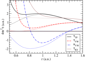
Figure 1: (color online) Comparison of all-electron and pseudopotential kinetic energy densities for the carbon atom. Shown are the radial probability density versus distance from nucleus for the Thomas Fermi (solid line), von Weizsäcker (dashed), and Kohn-Sham KED (lighter solid) as well as the quantity $u_{vW}$ (dot-dashed) defined in the text. The equivalent pseudopotential quantity for each is shown as a dotted line, matching at the cutoff radius 1.498 $a_{B}$.

The pseudopotentials for C are designed so that the pseudo-valence density matches the all-electron density after a cutoff radius of 1.498 $a_{B}$. This match is respected for the other quantities as well. However the pseudodensity and thus $\tau_{TF}$ continue to match the real density with reasonable agreement almost to the core-valence transition radius at about 0.8 $a_{B}$. The other pseudo-quantities deviate from their all-electron equivalents much more quickly, especially $\tau_{KS}$ and $u_{vW}$. In the all-electron case, core orbitals smooth out the density and thus reduce the magnitude of the $\nabla^{2}n\!<\!0$ peak in the valence shell, and they add extra terms to $\tau_{KS}$. The quantitative impact on $\nabla^{2}n$ is quite significant: the region of peak negative $\nabla^{2}n$ (the valence shell charge concentration or VSCC in QTAIM analysis) is broader in extent and the position of the critical point about 40% closer to the nucleus than in all-electron calculations. The maximum negative value of $\nabla^{2}n$ is typically three times larger than its all-electron equivalent, with similar errors for the VSCC’s of molecules. Plots shown below for $\nabla^{2}n$ and $\tau_{KS}$ in molecules do faithfully reproduce the qualitative topological features of the all-electron case, and are quantitatively accurate at bond centers and asymptotically; but they must be treated with caution with respect to other quantitative details.

IV.2 Electronic Structure: molecules

Figures 2, 3, 4 and 5 show contour plots for the density and related quantities for pseudopotential models of several of the molecules of the test set: $\mathrm{C_{3}H_{4}}$, $\mathrm{C_{2}H_{2}O_{2}}$ and $\mathrm{SiH_{4}}$. and SiO. In Fig. 2, we show in the first row (a) the ground-state pseudo-density $n$ and (b) the gradient factor $\left|\nabla n\right|^{2}/n$ that appears in the gradient expansion of $\tau_{KS}$ [Eq. (8)] and the von-Weizsäcker KED [Eq. (13)]. The second row shows (c) the Laplacian of the density $\nabla^{2}n$, and the gradient-expansion derived pseudoLaplacian [Eq. (15)] used in metaGGA’s. The third row shows (e) the Kohn-Sham KED $\tau_{KS}$ and (f), the Perdew-Constantin mGGA model for the same. All quantities are plotted in hartree atomic units; all except (a) are thus dimensionally energy densities. The other figures show subsets of this suite of data, as identified by subcaptions, for the other three molecules.

Each figure shows a two-dimensional slice through the molecule, with a color surface plot with values ranging from blue (minimum value shown) to red (maximum). The numerical scales for the surface plots are shown in the bar to the right of each subplot. Superimposed upon these are contour plots. Thicker contour lines for the Laplacian and pseudo-Laplacian [Fig. 2(c) and (d)] indicate the zero contour; the other four functions plotted are positive definite. The contours are adjusted to bring out details of bonding regions, and do not cover the atom cores. Contour values and ranges for the equivalent quantities of Laplacian and pseudo-Laplacian are identical, as are those for the two KED’s in subplots (e) and (f). Atoms and bonds in the plane of a plot are indicated by black dots and thick black lines; projections of out-of-plane atoms and bonds onto the plane of the plot are shown as open circles and thick dashed lines.

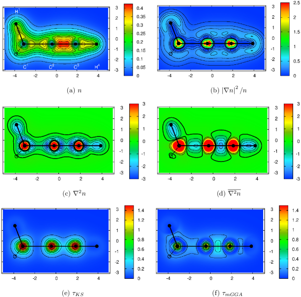
Figure 2: Functionals of the density for $\mathrm{C_{3}H_{4}}$ within the pseudopotential approximation, showing cut through the C–C–C bond axis and two hydrogens. In-plane atoms and bonds are shown as black disks and line segments; specific atoms are identified by labels. Out-of-plane ones shown as dashed lines and open disks. Contour levels for Laplacian (c) and pseudo-Laplacian of Eq. (15) (d) are identical, with thick contour at zero. Contour levels for mGGA KED (f) are the same as those of the Kohn-Sham KED (e).

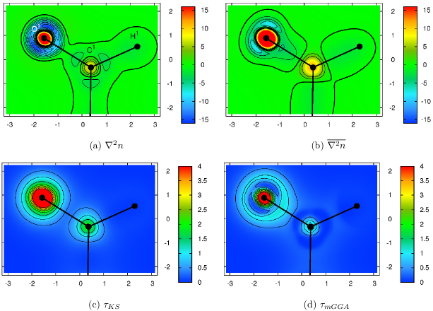
Figure 3: Functionals of the density for pseudo-$\mathrm{C_{2}H_{2}O_{2}}$, showing cut through the bond plane and an oxygen, carbon, and hydrogen atom. Details are the same as in Fig. 2.

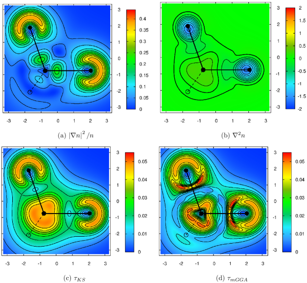
Figure 4: Functionals of the density for pseudo-$\mathrm{SiH_{4}}$, showing cut through a plane containing a Si atom at center and two tetrahedrally bonded hydrogens. Details are the same as in Fig. 2.

We start out with a discussion of the four direct measures of electronic structure – the density, $\left|\nabla n\right|^{2}/n$, $\nabla^{2}n$, and $\tau$ and consider the two approximations $\overline{\nabla^{2}n}$ and $\tau_{mGGA}$ in following subsections.

The subject of Fig. 2, $\mathrm{C_{3}H_{4}}$, is perhaps the richest example of the test set, illustrating several types of bonds. Three hydrogens (H¹ to H³) bond with a tetrahedral geometry to a carbon (C¹), which is joined to the second carbon ($C^{2}$) through a single bond, the second carbon shares a triple bond with the third (C³), and this is terminated with a final carbon-hydrogen bond. Our plots show a cut through the three central carbon pseudo-atoms aligned along the $x$-axis and one hydrogen on either end; the other two hydrogens extend out on either side of the far left-hand side of the plane.

The valence particle density (a) shows some features common to each molecule of the set. As in the single-atom case (Fig. 1), the density tends smoothly to a minimum at the center of each carbon pseudo-atom. In contrast, the hydrogen atom has no core electrons and the effect of the pseudopotential is simply to smooth out the cusp in the density at the nucleus. The highest electron density is thus naturally within bonds – especially the triple bond ($\mathrm{C}^{2}-\mathrm{C}^{3}$). The gradient-squared of the density (b) is nearly zero in regions with bonding, where the Laplacian (c) shows most structure, and is largest in the pseudo-atom core and at the edges of the molecule where $\nabla^{2}n$ is zero, as indicated by the thicker contour line in (c). The Laplacian is negative almost entirely along the center except for the interior of each carbon pseudo-atom. This is a hallmark of covalent bonding in QTAIM analysis Bader (1991); Bader and Essén (1984) – the center of a bond is a saddle critical point for the particle density, with a negative value for a covalent bond because of the the buildup of charge between atoms. The value of $\nabla^{2}n$ at the C¹–C² bond critical point is -0.700 and that for C²–C³ is -1.143, reasonable values for C–C bonds. Bader and Essén (1984) $\nabla^{2}n$ is positive in the pseudo-atom core, where the density is at a local minimum, and in the classically forbidden region far from the molecule. The Kohn-Sham kinetic energy density (e), is the smoothest and least structured of the measures of the Kohn-Sham system shown. As its relationship to the electron density is nontrivial, it not surprisingly appears to have little apparent correlation with it. It is primarily concentrated in the pseudo-atom cores with a strong peak at the center of the pseudo-atom. This follows the qualitative trend of the KED of all-electron systems, Jacobsen (2013) except for the absence of shell structure. Otherwise it is significantly larger in the triple bond than in the single bonds, where it is nearly zero.

Fig. 3 shows Laplacian and KED quantities for the $\mathrm{C_{2}H_{2}O_{2}}$ pseudo-molecule. This has a trigonal-planar form with a line of symmetry through the center of the molecule. The oxygens share polar double bonds with the carbons, and the carbons form covalent single sp² bonds with each other and the hydrogens. There are two lone pairs of electrons present on each oxygen. The plot shows one oxygen, carbon and hydrogen, and part of the C–C bond at the bottom of the plot. The single C–C and C–H bonds are very similar to those in $\mathrm{C_{3}H_{4}}$, so that the scale is adjusted to favor the oxygen atom which has a much larger density and KE density.

The C–O bond, being polar, exhibits several features not seen in $\mathrm{C_{3}H_{4}}$. The density gradient is nonzero in the bond – the push of density towards the more electronegative oxygen causes a local saddle point in the gradient on the oxygen side. VSCC lobes due to two sets of unpaired electrons are identifiable on the oxygen, but none on the bond axis, a reflection of the change in character of the bond. However, the VSCC lobes of peak negative $\nabla^{2}n$ (a) around the carbon atom are similar to those of the pure covalent bond. The kinetic energy density, as for $\mathrm{C_{3}H_{4}}$, is concentrated in atom cores with little contribution from within the bond, and thus the bond’s polar character causes no observable change from that of the covalently bonded system.

Next we consider $\mathrm{SiH_{4}}$, a nearly spherical molecule closely resembling a filled-shell atom in structure. It exhibits straightforward tetrahedral bonding, with sp³ hybridization of the silicon orbitals and covalent Si-H bonds. Fig. 4 shows a cut through a plane containing three of the atoms (H, Si, H) of the pseudo-molecule. A pair of hydrogen atoms is located above and below the plot plane as indicated by the open circles.

An item of interest is the comparison between $\tau_{KS}$ (c) and $\left|\nabla n\right|^{2}/n$ (a). Recalling that the von Weizsäcker KED [Eq. (13)] is $\left|\nabla n\right|^{2}/8n$, we set the color scales of (a) and (c) to an exact 8:1 ratio so that a comparison of $\tau_{KS}$ relative to $\tau_{vW}$ can be made. (For the other molecules, such a scheme wipes out almost all information about the gradient of the density, because $\tau_{KS}$ is much larger than $\tau_{vW}$.) Here it is apparent that the Kohn-Sham KED reaches the von Weizsäcker limit everywhere in the vicinity of a hydrogen atom. This seems reasonable in that each hydrogen atom has a single occupied orbital, and is in a sense a paradigm for the von Weizsäcker limit in fermionic systems. The Laplacian for the Si–H bond (b) heavily emphasizes the H atom because of the more dispersed nature of Si valence orbitals as compared to those of H.

A final example from the test set is SiO, which features a double bond that should be polar covalent given an electronegativity difference of 1.6. Fig. 5 shows a surface plot of the Laplacian of the density for a cut through the pseudo-molecule Si–O bond. Other quantities are available for SiO in the supplementary material. The valence electrons that participate in this bond heavily favor oxygen, the more electronegative atom, leaving the silicon atom hypovalent. CCC (2002)

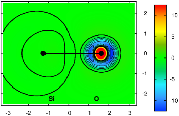
Figure 5: Laplacian of the density for pseudo-SiO, showing cut through the bond axis. Details same as for Fig. 2(c).

The zero contour (thicker contour) of $\nabla^{2}n$ is of interest for this system as it indicates a bond topology qualitatively different from the other cases. The orientation of the zero contour, crossing the bond perpendicularly to the bond axis, indicates that $\nabla^{2}n\!>\!0$ in the bond center – specifically in the region between the two closed contours surrounding Si and O respectively. This indicates in QTAIM analysis that the bond is ionic; the maximum value of $\nabla^{2}n\!=\!0.194$ is comparable to that of NaCl. Bader and Essén (1984) There is essentially a catastrophe in the topology of the zero contours whereby the Si–O bond cannot be mapped to a polar-covalent geometry, such as the C–O bond in $\mathrm{C_{2}H_{2}O_{2}}$, without breaking and rejoining contours.

Surface plots for the last two molecules of the AE6 test set ($\mathrm{S_{2}}$ and $\mathrm{C_{4}H_{8}}$) are not shown in this paper but are available in the supplementary data. sup Although they repeat themes already discussed for the other molecules, they have individual characteristics that should benefit from further investigation. The triplet ground state of $\mathrm{S_{2}}$, with a double bond and two lone pairs per atom, is similar in structure to $\mathrm{C_{3}H_{4}}$ and $\mathrm{C_{2}H_{2}O_{2}}$. Nevertheless, the KED shows interesting structure near the valence shell peak and in the bond. Cyclobutane ($\mathrm{C_{4}H_{8}}$) is a cyclic molecule with a ring of four carbons and two hydrogens bonded to each. Unique to this system is the low-density region inside the carbon ring where the gradient of the density is zero but the Laplacian and KED are not. This topology is similar to that of the bond-center of a nearly dissociated molecule, and not found elsewhere (at equilibrium geometry) in the test set. Such regions have been of interest for QTAIM analysis Bader (1991) and may provide a glimpse into how well approximated KED’s perform in predicting binding.

IV.3 Gradient expansion for the Laplacian

The subfigure (d) of Fig. 2 and (b) of Fig. 3 show the pseudo-Laplacian $\overline{\nabla^{2}n}$ [Eq. (15)] which approximates the Laplacian in terms of the electron density, its gradient and the kinetic energy density. Up to a small correction proportional to $\left|\nabla n\right|^{2}/n$, this quantity is simply $6(\tau_{KS}\!-\!\tau_{TF})$; given that $\tau_{TF}$ is a power of the particle density, it interprets the Laplacian as roughly a measure of the difference between the kinetic energy and particle densities. As seen especially in Fig. 2, our data support this qualitative picture. The Laplacian (c) is positive and large in the carbon pseudo-cores, precisely where the kinetic energy density (e) is largest and the charge density (a) is at a minimum; it is most negative in the bond regions where the situation is reversed. As a result, $\overline{\nabla^{2}n}$, plotted in (d) with the identical set of contours as $\nabla^{2}n$, captures the basic qualitative trends of this quantity, and on average, its relative magnitude in each bond. In contrast, the zero contour of $\nabla^{2}n$ and $\overline{\nabla^{2}n}$, shown as thicker black contours, have qualitatively different topologies. However, it seems reasonable to expect that, given their qualitative similarity, they could produce similar results if used as parameters in a functional for an integrated quantity such as the exchange energy. Notably, the contour of $\overline{\nabla^{2}n}\!=\!0$ closely matches the shape of the $1/2$-contour of the LOL, a close equivalent when density gradients are small. Jacobsen (2013)

A check on the quality of this approximation can be obtained by the sum rule for $\nabla^{2}n$. Since it is an exact derivative, the integral of $\nabla^{2}n$ over the entire unit cell should be exactly zero. While the integral for $\nabla^{2}n$ is zero to within round-off error, that for $\overline{\nabla^{2}n}$ ranges from about 0.1 hartree for $\mathrm{SiH_{4}}$ to about 20 hartree for the largest molecules. This is a reflection of the very large difference between the integrated Kohn-Sham kinetic energy and that of the Thomas-Fermi approximation. Energy densities can differ by several orders of magnitude in the pseudo-atom cores, an effect beyond the scale of our surface plots, but clearly shown in the log plots in Sec. IV.5.

IV.4 The mGGA model for the kinetic energy density

The final quantity for which we have made surface plots is the mGGA orbital-free KED. Perdew and Constantin (2007) It is shown for three molecules, subfigure (f) of Fig. 2 and (d) of Fig. 3 and 4, with contours and color scale that duplicate those of the Kohn-Sham KED. The agreement between the two is generally not good. For $\mathrm{C_{3}H_{4}}$ (Fig. 2) the mGGA, like the true KED, peaks in the pseudo-atom core, but is much smaller in magnitude. It is too large in the center of bonds, particularly the C²–C³ multiple bond. The most striking difference is the dramatic drop in magnitude in the mGGA in the region of peak valence charge concentration surrounding each carbon atom. The shape of these zeroed-out regions correlates with the VSCC lobes of the Laplacian accentuating regions of peak density. The identical pattern shows up in $\mathrm{C_{2}H_{2}O_{2}}$ (Fig. 3), with the KED zeroing out in VSCC regions for both oxygen and carbon, almost perfectly matching the contours of $\nabla^{2}n$ for the two lone oxygen pairs. This pattern occurs around the carbon atoms of $\mathrm{C_{4}H_{8}}$, the two lone pairs of each S atom in $\mathrm{S_{2}}$ and of the oxygen atom of SiO, indicating a global trend.

$\mathrm{SiH_{4}}$, shown in Fig. 4, is a case in which the mGGA works. In this case, much of the system is already very close to the von Weizsäcker limit, which the mGGA is designed to capture exactly. Moreover, errors in the mGGA in different regions, such as in the Si atom core and near the hydrogen atom, almost exactly cancel, leading to a qualitatitively much better match of the mGGA to the exact KED than for the other five cases. (Notably, the Si pseudo-atom lacks the strong VSCC lobes associated with unusually low mGGA KED in $\mathrm{C_{3}H_{4}}$ and $\mathrm{C_{2}H_{2}O_{2}}$.)

IV.5 Plots through bond axes

In this section, we focus on the quantitative comparison of various models for the kinetic energy density, for which linear plots are convenient. We plot the enhancement factor $F_{S}=\tau/\tau_{TF}$, which avoids excessive differences in scale between atoms. We are also interested in the measure of electron localization $\alpha$ [Eq. (16)], that can also be thought of as the Pauli contribution to the enhancement factor.

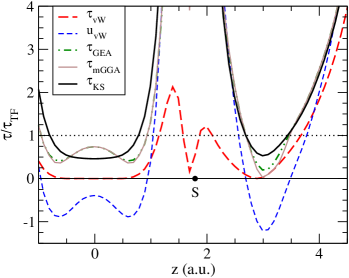
Figure 6: (color online) The enhancement factor $F_{S}=\tau/\tau_{TF}$ for the Kohn-Sham kinetic energy density (solid black line) and various orbital-free models, within the pseudopotential approximation, versus position along the bond axis $z$ for $\mathrm{S_{2}}$. Also shown is $F_{S}$ for $u_{vW}\!=\!\nabla^{2}n/4$. The Thomas-Fermi result, trivially one, is shown as a dotted line. Location of the sulfur atom noted by solid dot.

In Fig. 6 we show $F_{S}$ of several model KED’s for the pseudopotential approximation to the disulfur molecule $\mathrm{S_{2}}$ as a function of displacement $z$ from the molecule center along the bond axis. The focus is on a single sulfur pseudo-atom, marked by the black dot on the $F_{S}\!=\!0$ axis; the molecule has a mirror-symmetry plane through the bond center at $z\!=\!0$. The Thomas-Fermi result is the horizontal line $F_{S}\!=\!1$. The von Weizsäcker enhancement factor, $\tau_{vW}/\tau_{TF}\!=\!5p/3$, is nearly zero in the bond region and again at the density peak associated with the lone pair behind the bond. The related expectation $u_{vW}$ has an enhancement factor equal to $10q/3$. It is negative in the covalent bond and the lone-pair behind the sulfur atom, and positive in the pseudopotential core and asymptotically.

Both the gradient expansion $\tau_{GEA}$ and the more sophisticated $\tau_{mGGA}$ are positive definite, in agreement with the required behavior of $\tau_{KS}$. Each is at a minimum in the bond and lone-pair regions, reach local maxima in the core and tend to $\infty$ asymptotically. However, $\tau_{KS}$ is smooth and featureless, lacking the oscillatory structure of the gradient and Laplacian of the density. The mGGA, where it differs from the GEA, does a slightly worse job in describing the Kohn-Sham value. In the lone-pair region around $z\!=\!3$ a.u., it suffers from the extinction effect seen in the surface plots for $\mathrm{C_{3}H_{4}}$ and $\mathrm{C_{2}H_{2}O_{2}}$. Here, $u_{vW}/\tau_{TF}\!<\!-1$, equivalent to $q\!<\!-0.3$, which proves to be a significant criterion for this problem to occur in the mGGA. Overall, the mGGA fares better for $\mathrm{S_{2}}$ than for other molecules, perhaps because this error in its enhancement factor is cancelled by a reverse effect at the center of the double bond. The electron-localization measure $\alpha$, not shown in Fig. 6, is available in Fig. S-1 of the supplementary material. sup

Fig. 7 shows enhancement factors for pseudo-SiO. As noted previously, this is the most polar molecule in the test set and gives a structural contrast to the more covalent molecules. As such we focus on $\tau_{vW}$ and $u_{vW}$ as stand-ins for the gradient and Laplacian of the density, and related variables $p$ and $q$, as compared to the Kohn-Sham KED.

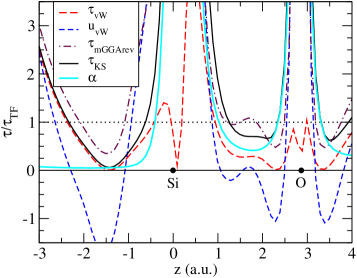
Figure 7: (color online) The enhancement factor $F_{S}\!=\!\tau/\tau_{TF}$ for the Kohn-Sham and von Weizsäcker KED’s, compared to the difference between the two, $\alpha$, versus position along the bond axis $z$ for pseudo-SiO. Also shown is $F_{S}$ for $u_{vW}\sim\nabla^{2}n$ and the mGGArev discussed in Sec. V.3; dotted line indicates the Thomas-Fermi result. Location of each atom on bond axis noted by a solid dot.

The gradient squared of the density ($\sim\!\tau_{vW}$) does not vanish in the bond, as the density steadily increases from the Si valence shell to the O. The Laplacian ($\sim\!u_{vW}$) is positive at the center of bond, the QTAIM indication of ionic character. It is also instructive to plot the electron localization measure $\alpha$, shown as the lighter (cyan) solid line in Fig. 7. In the SiO bond, this measure approaches 0.5, equivalent to an ELF of 0.67, which is the value approached by the other double bonds in the test set. A more telling structure occurs behind the Si atom, where $\alpha$ falls nearly to zero over an extended region of space. The value $\alpha\!\sim\!0$ (ELF of one) indicates that there is at most one occupied orbital so that $\tau_{KS}$ reaches von Weizsäcker limit almost perfectly. It also coincides with an abnormally low minimum in $\tau_{KS}$. This probably is a reflection of the hypovalent character of Si in this molecule; however restricting the plot to the bond axis also eliminates the contribution of two $\pi$-bond orbitals to the KED.

Fig. 8 shows enhancement factors for the $\mathrm{C_{3}H_{4}}$ pseudo-molecule, for points through the axis joining the three C atoms and the on-axis terminal hydrogen (H⁴). We plot $F_{S}$ on a log scale to focus on the situation at low densities, characterized by the carbon pseudo-atom cores and the asymptotic region far from the molecule.

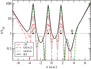
Figure 8: (color online) The enhancement factor $F_{S}=\tau/\tau_{TF}$, plotted on a log scale for various kinetic energy densities versus position along the carbon-carbon bond axis $z$ for the $\mathrm{C_{3}H_{4}}$ (propyne) pseudo-molecule. Location of atoms on axis noted by a solid dot. The Thomas-Fermi limit $F_{S}\!=\!1$ is shown as dotted line.

The asymptotic behavior of the Kohn-Sham and other KED’s is dominated by linear trend of $\log{(F_{S})}$ to infinity far from the molecule ($|z|\!>\!5$). This is consistent with exponential decay of the charge density – and with $\tau_{TF}\sim n^{5/3}$ decaying more rapidly than any other model. The three orbital-free models shown – the von Weizsäcker model, the GEA and the mGGA – have roughly the same decay constant, and for the most part match up quite well with the Kohn-Sham value. Interestingly, the GEA is the best predictor of $\tau_{KS}$, performing better than the mGGA almost everywhere. The von Weizsäcker form almost matches the Kohn-Sham case for the asymptotic edge near the lone hydrogen ($z\!>\!5$) – an indication that a single frontier orbital dominates the behavior of $\tau_{KS}$ in this region. On the other edge of the bond axis ($z\!<\!-5$) $\tau_{KS}$ is roughly twice as large as $\tau_{vW}$. This area sees the intersection of three frontier orbitals, one from each of the three C–H bonds that form tetrahedrally off the central bond axis. This is enough to detach $\tau_{KS}$ from the single occupied-orbital limit.

An interesting story also occurs in the pseudopotential cores of the carbon atoms, with similar behavior seen for other atoms that have had core electrons replaced by pseudopotentials. Although this is arguably the least physical region of the molecule, it does represent one of rapidly varying low density, but negligible density gradient, a topology that occurs in noncovalent bonds and the interstitial regions of solids. Here again the Kohn Sham KED is much larger than the Thomas Fermi value – as noted before, the charge and kinetic energy densities of our pseudopotential systems observe a kind of complementarity, with one being large where the other is small. Of the three model KED’s, it is the GEA that reproduces the KS value most accurately. The von Weizsäcker model peaks at the edge of the core region where $\left|\nabla n\right|^{2}$ is large, disappearing in the center of the pseudopotential core where it goes to zero. The GEA here closely follows $\nabla^{2}n$ which has a local maximum in the core and thus the correct qualitative behavior; surprisingly, the result is even quantitatively accurate. The mGGA trends more with $\tau_{vW}$, and is severely deficient in magnitude.

It is also useful for assessing approximate KED’s to plot the approximation to the electron-localization factor $\alpha$ obtained within a given model $\tau_{approx}$:

$$\alpha_{approx}=(\tau_{approx}-\tau_{vW})/\tau_{TF}.$$ (18)

Focusing again on $\mathrm{C_{3}H_{4}}$, which has the richest electronic structure of the test set, we plot in Fig. 9 the $\alpha$ for several model KED’s on a log scale versus position $z$ along the central bond-axis. For the exact Kohn-Sham $\tau$, we find three regions with $\alpha\!<\!1$, an indication of electron localization – the two carbon-carbon bonds and single terminating hydrogen atom. The other limit, $\alpha\!\gg\!1$, occurs inside the pseudo-atom cores and asymptotically. The degree of localization of each small-$\alpha$ region is consistent with the character of that region. It is weakest ($\alpha\!\sim\!0.5$) for the triple bond between the second and third carbons, stronger ($\alpha\!\sim\!0.3$) for the single bond between the first two carbon atoms and extreme ($\alpha\!\sim\!0.05$) for the final hydrogen atom where only a single orbital is occupied. As expected from the other figures shown, no approximate model does very well in these important situations.

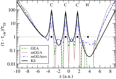
Figure 9: (color online) The electron localization measure $\alpha_{approx}=(\tau-\tau_{vW})/\tau_{TF}$, plotted on a log scale for various kinetic energy densities versus position along the carbon-carbon bond axis $z$ for the $\mathrm{C_{3}H_{4}}$ (propyne) pseudo-molecule. Location of atoms on axis noted by a solid dot. The Thomas-Fermi value $\alpha\!=\!1$ is shown as dotted line. The mGGArev is defined in Sec. V.

Two subtle order-of-limits issues come into play asymptotically. The approximate GEA and mGGA both do considerably worse in predicting the asymptotic trend of $\alpha$ in Fig. 9 than they do the enhancement factor of $\tau_{KS}$, in Fig. 8. $\alpha$ measures a difference between two models of $\tau$, and this difference is an order of magnitude smaller than the value of either model far from the molecule. It is thus a more sensitive probe of error in orbital-free models. Secondly, while the GEA has the correct asymptotic behavior (although consistently three times too large), the mGGA has incorrect behavior as $|z|\rightarrow\infty$. To understand this, note that $\alpha$ asymptotically can tend to anything from 0 to $\infty$. By the IP theorem, the numerator in Eq. (16) must vanish as the system tends to a one-electron state and $\tau_{KS}\!\rightarrow\!\tau_{vW}$, but the denominator also vanishes, as $n^{5/3}$, leaving the ratio undetermined. While the asymptotic value of $\alpha$ is one in the mGGA, for almost all the cases we have tested (SiO seems an exception) the observed limit is infinity. This perhaps indicates only that $\tau_{TF}$ is an infinitely bad predictor of $\tau_{Pauli}$ for a region in which the Thomas-Fermi approximation fails.

V Analysis

V.1 The GEA and asymptotic behavior of the KED

It is worth analyzing in some depth what happens in the region of asymptotic decay far from the molecule, as demonstrated especially in Fig. 8, and to some degree in Fig. 6. It is striking that $\tau_{KS}$ and $\tau_{GEA}$ match each other almost perfectly in this limit, within 3% at higher densities and no more than 15% at the lowest densities we can obtain. Consequently $\nabla^{2}n$ and its GEA-level approximation, $\overline{\nabla^{2}n}$, also agree almost exactly for this region. This close agreement occurs for all systems studied, for example, for SiO as one either moves away from the hypovalent Si atom or from the nearly filled O atom. This is quite surprising since the GEA is designed for a completely different situation, that of the slowly varying electron gas, which is presumably unsuitable for a classically forbidden region of space. Formally, the regime of validity of the slowly varying electron gas is for systems for which the inhomogeneity measures $p$ and $q$ are everywhere $\ll 1$. Obviously this criterion cannot be exactly met for a molecule, but one might expect that, in any extended region where these parameters are small, $\tau_{KS}$ should approach $\tau_{GEA}$. In fact, the opposite proves true: regions of space like covalent bonds, where $p$ and $q$ are consistently smallest, are where the GEA does the worst, while the classically forbidden asymptotic region, where both $p$ and $q$ are much greater than one, is where it performs best. (To compare with the quantities shown in Figs. 8 and 9, recall $\tau_{vW}/\tau_{TF}\!=\!5p/3$ and $u_{vW}/\tau_{TF}\!=\!10q/3$.) Thus we have to conclude that some other phenomenon than the physics of the slowly-varying electron gas must explain the agreement asymptotically.

It is not hard to find one, at least qualitatively. This region is characterized by an exponential decay of the density, $n\!\sim\!\exp{(-2kr)}$, where $k=\sqrt{2I}$ gives the decay rate of the frontier orbitals, which have the highest eigenenergy, equal to the ionization potential $I$, and tunnel farthest into the vacuum. As a result, the Kohn-Sham KED should behave as $k^{2}n$, decaying at a rate proportional to the local particle density. In contrast the Thomas-Fermi KED varies as $k_{F}^{2}n$ with $k_{F}\!\sim\!n^{1/3}$. The enhancement factor $F_{S}$ needed to correct $\tau_{TF}$ to the Kohn-Sham value then scales as $k^{2}/k_{F}^{2}$, causing the exponential growth seen in Figs. 6 and 8. It is notable that the second-order gradient expansion reproduces this scaling behavior. The inhomogeneity variable $p$ is equal to $(k/k_{F})^{2}$ for any exponentially decaying particle density – and $q$ is also, up to a correction due to curvature. The form of $\tau_{GEA}$ [Eq. (8)] gives its enhancement factor the correct limiting behavior as $r\!\rightarrow\!\infty$. In contrast, the fourth-order correction has terms which scale like $p^{2}\!=\!k^{4}/k_{F}^{4}$, which blow up exponentially as $r\!\rightarrow\!\infty$. And a GGA, a closed expression summing over all orders of the gradient expansion, is not necessary to capture order-of-magnitude trends and can actually be less accurate than the second-order GEA.

This is in stark contrast to what happens for the exchange energy: the energy density associated with a single frontier orbital behaves asymptotically as $(\frac{1}{2r})n$ while the LDA scales as $k_{F}n$. Applying the second-order gradient expansion to the LDA creates an exchange energy density that scales incorrectly as $(k^{2}/k_{F})n$ and a potential that diverges exponentially. A GGA is needed to produce an accurate exchange energy and a potential that is finite (if not with the correct $1/r$ form.) This contrast between the correction needed for LDA exchange $\sim n^{4/3}$ and Thomas-Fermi KED $\sim n^{5/3}$ contradicts the conjointness conjecture in its usual formulation – the same form of enhancement factor cannot be optimal for both cases.

V.2 Revisiting the mGGA

It is not hard to diagnose why the mGGA KED has difficulty modeling the molecular bond. The mGGA was tested primarily for closed-shell atoms and several model one-dimensional systems. Perdew and Constantin (2007) The most serious defects of the mGGA seen in the current study are associated with regions of of joint $\{p,q\}$ space that these systems do not access. The issue of vanishing KED is strongly correlated with regions where $p\!\sim\!0$ and $q$ is negative and of the order of unity, a combination that does not happen with atoms. Cancio and Wagner (2013) A second problem is the mGGA’s large underestimate in the pseudopotential core where $p\!\sim\!0$ and $q\!>>\!0$; in atoms, a large $q\!>\!0$ is associated with finite and normally large $p$, and occurs primarily in the asymptotic region far from the atom where both tend to $\infty$. loo While both these errors lead to underestimates of the KE, the former is a failure to model the KED in the valence shell of an atom or molecule and should have a large impact on the model’s ability to predict molecular structure.

The common thread here is the behavior of the KED as a function of $q$ for values of $p\ll|q|$ and near to zero. In Fig. 10 we plot the $p=0$ limit of the KED enhancement factor, $F_{S}(0,q)$, for several KED models as a function of the scale-invariant factor $q$. By definition, $F_{S}\!=\!1$ for $\tau_{TF}$, as shown by the dotted horizontal line. Likewise, the von Weizsäcker KED for $p\!=\!0$ is zero for all $q$. The $F_{S}$ of the fourth-order gradient expansion approximation reduces to $1+(20/9)q+(8/81)q^{2}$. This is nearly indistinguishable to the second-order gradient expansion, linear in $q$, because the fourth order coefficient is so small. The model of interest is the solid red line, that of Perdew and Constantin. It starts off with the gradient expansion and applies further constraints. First, the von Weizsäcker bound requires that the enhancement factor be greater than $F_{vW}$, in effect greater than zero. For $q\!<\!0$ the KED must transition fairly quickly from GEA-like behavior to zero, as the GEA breaks this constraint at $q\!\sim\!-0.45$. The second imposed limit is that the enhancement factor goes to $1+F_{vW}$ in the limit of large positive $q$, seen for example in our data in pseudo-atom cores, but not shown in Fig. 10.

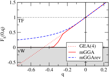
Figure 10: (color online) Kinetic energy density enhancement factor $F_{S}(p,q)$ for orbital free kinetic energy density models, plotted versus gradient-expansion parameter $q$ for $p\!=\!0$. Thomas-Fermi limit $(F_{S}\!=\!1)$ indicated by dotted line. Gray shaded region shows values of $F$ disallowed by the von Weizsäcker bound given by $F_{S}\!=\!0$.

The flaws in the mGGA seem to be caused by its implementation of these constraints. The most important, the extinction of KED for negative $q$ and small $p$, is clearly the result of a transition from $\tau_{GEA}$ to $\tau_{vW}$ that zeroes out the KED for $q\!<\!-0.30$, a value of $q$ achievable in the vicinity of an atomic lone-pair or a covalent bond, especially in a pseudopotential system. This transition scheme implicitly invokes an order of bounds as follows:

$$\tau_{GEA}\geq\tau_{KS}\geq\tau_{vW}$$ (19)

That is, it seeks an interpolation between the two limiting cases, which leaves very little room for smoothing out the transition. Wig It makes more sense to try an interpolation above the two limiting cases, assuming a constraint

$$\tau_{KS}\geq\mathrm{max}(\tau_{GEA},\tau_{vW}),$$ (20)

demonstrated by the blue dashed curve in Fig. 10. Such a transition is smoother and thus more physically appealing, and has the effect of enhancing rather than reducing the KED in high-density, low-$q$, regions. A smoother transition to zero should also produce a smoother kinetic energy potential which is important for a self-consistent density functional minimization. Abrupt changes in the enhancement factor of a Laplacian-based density functional can be disastrous when taking functional derivatives with respect to $\nabla^{2}n$, since these involve derivatives of the density up to $\nabla^{4}n$. Cancio, Wagner, and Wood (2012)

The mGGA model can also be improved by relaxing the large-$q$ cutoff that it imposes. As seen especially in Fig. 9, the mGGA clearly overcorrects for the regions where $q\!\gg\!1$, in the pseudo-atom core and asymptotically. In both cases, the second-order GEA is a better approximation to $\tau_{KS}$ and there is less motivation for a GGA correction to it than is the case for exchange.

V.3 Revision of the mGGA and application to atomization energy

We propose to make a revised mGGA following two simple points: imposing the von Weizsäcker lower bound by means of Eq. (20) and relying on the second-order gradient expansion otherwise. This satisfies the constraints for the two main limiting cases of the KED – that of delocalized electrons with slowly-varying density and that of strong electron localization, and otherwise keeps physically reasonable behavior for regions of high inhomogeneity – pseudo-atom cores and asymptotic decay. We first define a measure of electron localization $z$ that depends upon the difference between GEA and vW enhancement factors for the KED:

$$z=F_{GEA}-F_{vW}-1=\frac{20}{9}q-\frac{40}{27}p$$ (21)

The factor $z$ can be thought of as a poor-man’s electron localization factor – an orbital-free expression for the $\alpha$ used to describe electron localization in metaGGA’s and from which the ELF is constructed. We then look for the simplest possible asymptotic transition between $F_{GEA}$ and $F_{vW}$ that imposes the von Weizsäcker bound, which occurs for $z\!\leq\!-1$. Adapting a form recently used to construct a $\nabla^{2}n$-based exchange function Cancio and Wagner (2013) results in an enhancement factor

$$F^{mGGArev}_{S}=F_{vW}+1+z\left\{1-\exp{\left(\frac{1}{z}\right)}\left[1-H(z)\right]\right\}$$ (22)

where $H$ is the Heaviside step function. This is shown in Fig. 10 as a function of $q$ for $p\!=\!0$.

The limiting behavior of this correction can be characterized by three cases, roughly analogous to those defined by the ELF:

1. If $z\rightarrow 0$, then both $p$ and $q$ must become small. The density is slowly varying, and close to the homogeneous gas limit, typical of metallic bonds. In this case, $F_{S}$ goes to the gradient expansion form:

   $$F_{S}\!\sim\!F_{vW}+1+z=F_{GEA}$$ (23)

2. If $z\!<\!0$, this means that either $q$ becomes negative or $p\rightarrow+\infty$ with a finite $q$. In this case, $F_{S}$ approaches the von Weizsäcker limit:

   $$F_{S}\rightarrow F_{vW}+O(1/z).$$ (24)

   This is the proper description of a region with strong electron localization, such as a covalent bond.

3. If $z\!\gg\!0$, we get the same result as for $z$ small:

   $$F_{S}\rightarrow F_{GEA}.$$ (25)

   The primary situation for which this limit applies is an exponentially decaying density, for which $p\!\sim\!q\rightarrow\infty$ and $z\rightarrow 20q/27$.

The final case also describes a situation with $q\!\gg\!1$ and finite $p$, seen here in pseudo-atom cores, and in the transition between atomic shells in real atoms.

Also of interest for real atoms is the limit $q,z\!\rightarrow\!-\infty$ which occurs near the nucleus and is caused by the cusp in the electron density. The functional derivative $\delta\tau/\delta n({\bf r})$, used for the self-consistent determination of the charge density in OFDFT, must tend to $Z/r$ near the nucleus so as to cancel the $-Z/r$ contribution from the electron-nucleus potential. This behavior is exactly given by the functional derivative of $\tau_{vW}$, and thus by $\tau_{mGGArev}$ as well. The leading correction to $\tau_{vW}$ is of order $1/q$; its functional derivative is known to be finite, Umrigar and Gonze (1994) but it can cause a sizable error in the cusp of $\tau$ at the nucleus.

To evaluate the effects of this revised mGGA, we plot its enhancement factor for SiO in Fig. 7 and its approximation to $\alpha$ using Eq. (18) for propyne in Fig. 9. As shown in the latter, the mGGArev by construction follows the GEA curve almost everywhere in space – except for regions of electron localization, where it enhances the magnitude of the KED considerably over the GEA. It is thus an improvement over both GEA and mGGA. However the mGGArev overcorrects for situations of strongest electron localization. For the single C¹-C² bond of propyne, with a small $\alpha$ of 0.3, the mGGArev gives a modest average overcorrection. It severely overcorrects for the most localized situations, where $\alpha\!<\!0.1$: near the terminal H⁴ atom in propyne and behind the hypovalent Si atom in SiO. This problem may be ameliorated by tinkering with the rate of transition between GEA and vW limits in Eq. (22) – in the current form (Fig. 10), it is probably too slow. One region that shows little change from the mGGA is behind the C¹ atom ($z\!\sim\!-4$) in Fig. 9. This is not a region of electron localization since it feels the overlap of three neighboring C–H bond orbitals so the model has no criterion to correct for the error of the GEA.

In Table 3 we show errors with respect to the integrated Kohn-Sham KE averaged over the test set, as a measure of the overall quality of the models discussed in this paper. A net trend across all models is the underestimation of the KE by roughly 10%. Unfortunately, by the virial theorem, the total KE is equal in magnitude to the total energy, which varies from 3.5 hartree for the valence shell of $\mathrm{SiH_{4}}$ to 31 hartree for that of $\mathrm{C_{2}H_{2}O_{2}}$. Absolute errors in KE can thus be as large as several hartrees. While the second-order GEA is a modest improvement over the Thomas-Fermi result, the mGGA, in attempting to address the limitations of the GEA, actually loses some of the ground gained by it. The revised mGGA introduced here is more consistently an improvement. One situation in which it is not, $\mathrm{SiH_{4}}$, results in the maximum RE being three times the MARE, and an overestimate, not an underestimate. As shown in Fig. 4, this molecule is marked by a substantial region that is near the von Weizsäcker limit, $\alpha\!\sim\!0$, for which the mGGArev overestimates the KED. This again indicates a need for further exploration of how to manage the transition from delocalized to localized electronic systems.

	TF	GEA	mGGA	mGGArev	VT84F
MRE	-0.162	-0.112	-0.124	0.0021	0.229
MARE	0.162	0.112	0.139	0.0873	0.229
Max RE	-0.202	-0.159	-0.178	0.233	0.550

Table 3: Mean relative error (MRE), absolute relative error (MARE) and maximum relative error (Max RE) for various orbital-free estimates of the Kohn-Sham kinetic energy.

To further characterize the quality of our revised mGGA, we calculate the atomization energies of the AE6 test set. This helps gauge the extent to which systematic errors in the total energy are cancelled out in taking energy differences. This is done not self-consistently, using conventional PBE Kohn-Sham densities and bond lengths (Table 1). The results are shown in Table 4.

System	Exp.	KS	VT84F	mGGA-	mGGA	GEA	TF
				rev
$\mathrm{SiH_{4}}$	322.4	315.9	-178.1	-14.9	57.2	-183.8	-174.9
$\mathrm{S_{2}}$	101.7	124.4	140.9	17.7	-101.5	-72.1	-100.6
SiO	192.1	205.4	-4.8	-4.5	-169.3	-97.6	-213.7
$\mathrm{C_{2}H_{2}O_{2}}$	633.4	680.6	476.6	240.2	-422.8	-119.0	-416.6
$\mathrm{C_{3}H_{4}}$	704.8	726.6	581.9	572.3	24.2	115.9	35.7
$\mathrm{C_{4}H_{8}}$	1149	1175.3	1072.4	811.8	142.6	96.0	-53.3
MAE	–	23.0	182.1	246.8	595.5	560.7	671.1

Table 4: Atomization energies for the AE6 test set in kcal/mol. Shown are experimental values from Ref. Lynch and Truhlar, 2003, self-consistent Kohn-Sham results, and results of orbital-free models evaluated with the Kohn-Sham density. Also shown is the mean absolute error with respect to experiment.

First we note how far the Thomas-Fermi atomization energy is from experiment, with an MAE ten times worse than the LDA and over thirty times worse than the PBE Kohn-Sham models. It almost always fails to predict binding, at best giving a marginal binding energy. The second-order GEA does provide a modest improvement over the TF case, but again shows severe under-binding. By respecting the von Weizsäcker lower bound, the mGGA ought to significantly improve GEA atomization energies. Instead it performs worse for the majority of the test set, and in some cases worse than Thomas-Fermi. In constrast, the mGGArev does show the expected improvement over Thomas-Fermi and GEA. It binds all but one molecule, $\mathrm{SiH_{4}}$, the standout worst case in Table 3, and the one case that the mGGA binds. On average it removes 60% of the AE error of the TF and for one or two systems almost approaches the LDA in quality. However its MAE is still an order of magnitude worse than the PBE and a factor of three worse than the LDA.

To put these results in perspective, we perform calculations for the VT84F, Karasiev et al. (2013) a nonempirical GGA for the kinetic energy. This applies the key constraints of the mGGA – respecting the gradient expansion in the small-$p$ limit and requiring the von Weizsäcker constraint for all $p$; in addition it enforces the non-negativity Levy and Ou-Yang (1988) of the Pauli potential, $\delta\tau_{Pauli}/\delta n({\bf r})\geq 0$. The VT84F total kinetic energy (Table 3) is by a large margin the least accurate of all models considered, including the Thomas-Fermi model. However it has the overall best prediction of atomization energies (Table 4), and fails significantly only for $\mathrm{SiH_{4}}$. It may be hard to enforce both the GEA and the constraint $\tau>\tau_{vW}$ with only access to $\left|\nabla n\right|^{2}$ as a variable and not overestimate the total KE. However enforcing constraints on the potential – an infinitesimal energy difference – seems to help for predicting accurate finite-energy differences. It is reassuring that the simple metaGGA we present here is comparable in quality to the VT84F without (as yet) taking the potential into consideration.

VI Discussion and Conclusions

We present highly converged DFT calculations for the AE6 test set of molecules, within a plane-wave pseudopotential approach. We use these to visualize the Kohn-Sham kinetic energy density and related quantities that are ingredients of modern DFT’s, specifically metaGGA models for the exchange-correlation energy, and orbital-free models for the KED. By providing a highly accurate map between density and kinetic energy density for physically reasonable model systems, our data enables the use of visualization techniques employed in the qualitative analysis of electronic structure to test approximations to this critical ingredient for DFT. The pseudopotential method works especially well in characterizing the classically forbidden region far from nuclei, and is reasonable in its description of bonds; its main limitation is the loss of knowledge of the core region, most importantly, the character of the core-valence transition that plays a key role in determining bond lengths.

The choice of the AE6 test set does not break new ground in visualization of electronic structure, but does an excellent job of illustrating many of the lessons learned from QTAIM and other visualization approaches, particurly the role of $\nabla^{2}n$ in understanding valence electronic structure and the KED in measuring electron localization. The SiO molecule is perhaps of most interest structurally, given the relationship between the hypovalent character of Si and the strong indication of electron localization in the Si valence shell; also of interest is the identification of the bond as ionic rather than polar covalent by QTAIM criteria.

A major finding of the paper is the surprising success of the gradient expansion expression for the Kohn-Sham KED. The gradient expansion approximation $\nabla^{2}n\!\sim\!6(\tau_{KS}\!-\!\tau_{TF})$ used in modern metaGGA’s is at least qualitatively very good – $\nabla^{2}n$ to some degree picks up the complementary behavior of the kinetic and particle densities, and detects regions where one is larger than the other. Rather surprisingly, this approximation is the most accurate in the lowest density regions, in the classically forbidden regions far from nuclei. This is because it has the exact asymptotic behavior with respect to distance from nuclei and not too bad quantitative values for all systems considered.

The asymptotic exactness of the GEA, although not news, is worthy of note since it points out the limitations of the idea of conjointness between exchange-correlation and kinetic energy functionals, both as a conjecture and as a design philosophy. Lessons learned in designing functionals for the former case do not necessarily transfer over to the latter. The very different behavior of the gradient expansion for exchange in the asymptotic limit necessitates a fundamentally different functional form for exchange energy GGA’s and kinetic energy GGA’s. The gradient expansion of the former must be controlled by some form of cutoff at large values of reduced density gradient $p$ while that of the latter, as best we can see, is better off mostly untouched.

A second point underscores the difficulty in building orbital-free models of the KE – the gradient expansion behaves worst in describing “slowly varying” regions of space – where the inhomogeneity parameters $p$ and $q$ used to describe it are small. For the KE density, there seems not to be a good “semilocal” approximation for real systems – one cannot rely on $p$ and $q$ being small locally to predict that the gradient expansion should hold locally, in contrast with the XC energy density. When taken separately, exchange and correlation energy densities have similar problems to those we see here for the KED; however, there is a notable cancellation of error between the two that makes semilocal approximations work better than might be expected. Hol What the KED lacks then is a companion mechanism such as correlation by which deviations from the GEA can be cancelled out. This failure does not contradict the idea of the gradient expansion. The limit in which it is exact is that of globally small $p$ and $q$, with the result of delocalized electronic orbitals almost everywhere, a condition that is not met by any molecule.

The other major finding of this paper relates to the Perdew-Constantin mGGA model of the kinetic energy density. We have found a number of problems which degrade its performance with respect to the Thomas-Fermi model. Its description of the KED in regions of high inhomogeneity and low density are less effective than the simpler second-order GEA. More importantly, it is subject to an “extinction” effect for large negative values of the reduced Laplacian $q$, causing it to plummet to zero in regions of covalent bonding. This effect is caused by the particular form used in the imposition of the constraint $\tau\!>\!\tau_{vW}$, which becomes important in regions of electron localization, such as covalent bonds. It is aggravated by the use of pseudopotentials, which exaggerate the magnitude of negative-$\nabla^{2}n$ or VSCC regions in comparison to their all-electron counterparts. The correlation between this effect and electron localization seems responsible for the poor binding seen with this model. The formation of bonds can reduce electron localization and thus reduce the extinction effect relative to the isolated atom case, leading to a lack of error cancellation in taking energy differences. Notably, the cases in which the mGGA gives improved binding energies, $\mathrm{SiH_{4}}$ and $\mathrm{C_{4}H_{8}}$, are the ones with exclusively single bonds and thus roughly the same degree of electron localization in molecule and atom.

This work points to several avenues of future research. The mGGArev form we propose for the KED is the simplest, not best, form that can fit the constraints imposed in Sec. V and should perhaps be used not as a finished functional but as an indication of how to proceed in developing one. Particularly, the use of an “orbital-free ELF”, using derivatives of the density to approximate the ELF and its ability to distinguish between different kinds of bonds, seems worthy of further investigation. However, in its current form, our model regresses on the mGGA’s capacity to handle covalently bonded hydrogen atoms and other situations of nearly perfectly localized electrons. Notably, our proposed constraint, that $\tau\!>\!\tau_{GEA}$ when $\tau\!\rightarrow\!\tau_{vW}$, is not universal – it fails for the 1s shell of atoms, as shown in Ref. Perdew and Constantin, 2007. Not surprisingly, the mGGA functional, with $\tau\!<\!\tau_{GEA}$ in this limit was arrived at partly through the consideration of this case. However our constraint does appear to be valid for any other shell of an all-electron atom – and it is responsible for our current revision’s relative success in predicting binding energies of the AE6 test set. Any more sophisticated model will thus have to ameliorate somehow the problems for hydrogen encountered by the mGGArev while keeping its nice features for bonding.

A second notable issue is the large deviation of $\nabla^{2}n$ and $\tau_{KS}$ obtained with pseudopotentials from their all-electron values just inside the pseudopotential cutoff radius. As noted earlier, the resulting exaggeration of the negative value of $\nabla^{2}n$ in VSCC’s contributes to the failure of the mGGA to predict binding in pseudopotential systems. But, given the sudden switching behavior that the mGGA shows for negative $q$ (Fig. 10), it is quite possible that with the smaller $q$ values of all-electron systems, this effect would not be an issue. This raises the question of how much pseudopotentials that have been constructed to match valence density alone can be trusted in metaGGA or OFDFT applications that rely upon variables that are more sensitive to changes in electronic structure.

In the big picture, the ability to get orbital-free DFT’s that are competitive with Kohn-Sham approaches remains a challenge. However, some progress towards functionals useful in extreme situations where Kohn-Sham approaches are impractical may yet be done with metaGGA’s working with semilocal properties of the density. Visualization can be a useful tool in this process, fruitfully bringing together strands of qualitative and quantitative thinking about electronic structure.