A martingale analysis of first passage times of time-dependent Wiener diffusion models

Abstract

Research in psychology and neuroscience has successfully modeled decision making as a process of noisy evidence accumulation to a decision bound. While there are several variants and implementations of this idea, the majority of these models make use of a noisy accumulation between two absorbing boundaries. A common assumption of these models is that decision parameters, e.g., the rate of accumulation (drift rate), remain fixed over the course of a decision, allowing the derivation of analytic formulas for the probabilities of hitting the upper or lower decision threshold, and the mean decision time. There is reason to believe, however, that many types of behavior would be better described by a model in which the parameters were allowed to vary over the course of the decision process.

In this paper, we use martingale theory to derive formulas for the mean decision time, hitting probabilities, and first passage time (FPT) densities of a Wiener process with time-varying drift between two time-varying absorbing boundaries. This model was first studied by Ratcliff (1980) in the two-stage form, and here we consider the same model for an arbitrary number of stages (i.e. intervals of time during which parameters are constant). Our calculations enable direct computation of mean decision times and hitting probabilities for the associated multistage process. We also provide a review of how martingale theory may be used to analyze similar models employing Wiener processes by re-deriving some classical results. In concert with a variety of numerical tools already available, the current derivations should encourage mathematical analysis of more complex models of decision making with time-varying evidence.

1 Introduction

Continuous time stochastic processes modeling a particle’s diffusion (with drift) towards one of two absorbing boundaries have been used in a wide variety of applications including statistical physics (Farkas and Fulop, 2001), finance (Lin, 1998), economics (Webb, 2015), and health science (Horrocks and Thompson, 2004). Varieties of such models have also been applied extensively within psychology and neuroscience to describe both the behavior and neural activity associated with decision processes involved in perception, memory, attention, and cognitive control (Heath, 1992; Ratcliff and Rouder, 1998; Ratcliff and McKoon, 2008; Simen et al., 2009; Gold and Shadlen, 2001, 2007; Brunton et al., 2013; Feng et al., 2009; Shadlen and Newsome, 2001; Diederich and Oswald, 2014, 2016); for reviews see (Ratcliff and Smith, 2004; Bogacz et al., 2006; Busemeyer and Diederich, 2010).

In these stochastic accumulation decision models, the state variable $x(t)$ is thought to represent the amount of accumulated noisy evidence at time $t$ for decisions represented by the two absorbing boundaries, that we refer to as the upper ($+$) and lower ($-$) thresholds (boundaries). The evidence $x(t)$ evolves in time according to a biased random walk with Gaussian increments, which may be written as $dx(t)\sim\text{Normal}(\mu\;dt,\sigma^{2}\;dt)$, and a decision is said to be made at the random time $\tau$, the smallest time $t$ for which $x(t)$ hits either the upper threshold ($x(\tau)=+\zeta$) or the lower threshold ($x(\tau)=-\zeta$), also known as the first passage time (FPT). The resulting decision dynamics are thus described by the FPT of the underlying model. In studying these processes one is often interested in relating the mean decision time and the probability of hitting a certain threshold (e.g. the probability of making a certain decision) to empirical data. For example, these metrics can offer valuable insight into how actions and cognitive processes might maximize reward rate, which is a simple function of the FPT properties (Bogacz et al., 2006).

However, not all decisions can be properly modeled if parameters are fixed throughout the duration of the decision process. Certain contexts can be better described by a model whose parameters change with time. In this article we analyze the time-dependent version of the Wiener process with drift between two absorbing boundaries, building on recent work that is focused on similar time-varying random walk models (Hubner et al., 2010; Diederich and Oswald, 2014). After reviewing how martingale theory can be used to analyze and re-derive the classical FPT results for the time independent case, we calculate results for the time-dependent case. The main theoretical results are presented in §5.2, where we provide closed form expressions for threshold-hitting probabilities and expected decision times. In D, we also describe how our methods can be applied to the more general Ornstein-Uhlenbeck (O-U) processes, which are similar to the Wiener diffusion processes albeit with an additional “leak” term. We conclude with a summary of the results and a discussion of how the present work interfaces with other similar analyses of time-varying random walk models.

2 Notation and terminology

Here we introduce the notation and terminology for describing the model we analyze, which is a Wiener process with (time-dependent) piecewise constant parameters. This simple stochastic model, and others close to it, have been studied before (Ratcliff, 1980; Heath, 1992; Smith, 2000; Diederich and Busemeyer, 2003, 2006; Diederich and Oswald, 2014; Bogacz et al., 2006; Wagenmakers et al., 2007), although the reader should note that our parameterization differs from that of some previous studies. Before describing the model, we first review the case where parameters are unchanging with time. In order to easily discuss this simpler model alongside the main time-dependent model analyzed in §5, we use the terms single-stage model and multistage model, respectively. Readers familiar with the popular Diffusion Decision Model of Ratcliff and McKoon (2008) should be aware that parameters in our model do not vary randomly trial-to-trial. Readers familiar with Bogacz et al. (2006) should be aware that the single-stage model (1) is equivalent to what Bogacz et al. (2006) call the “pure” Drift Diffusion Model.

2.1 The single-stage model/process with constant parameters

Consider the stochastic differential equation (SDE):

$$dx(t)=\mu\,dt+\sigma dW(t),\,\,\,x(t_{0})=x_{0},$$ (1)

where parameters $\mu$ and $\sigma$ are constants referred to as the drift and diffusion rates, respectively; $x_{0}$ is the initial condition (the initial evidence or starting point) of the decision process; and $\sigma dW(t)$ are independent Wiener increments with variance $\sigma^{2}dt$. This simple stochastic model has successfully modeled the evolution of evidence between two decisions during a two-alternative forced choice task (Ratcliff and Rouder, 1998; Bogacz et al., 2006; Ratcliff et al., 2016), so that (1) can be interpreted as modeling a decision process in which an agent is integrating noisy evidence until sufficient evidence is gathered in favor of one of the two alternatives.

A decision is made when the evidence $x(t)$ crosses one of the two symmetric decision thresholds $\pm\zeta$ for the first time, also referred to as its first passage time (FPT). In other words, a decision occurs the instance $x(t)$ crosses and is absorbed by one of the two boundaries. The two boundaries each correspond to one of the two possible decisions for the task. We will refer to the absorbing thresholds at $+\zeta$ and $-\zeta$ as the upper and lower decision boundaries/thresholds. To contrast with the next section, we will sometimes refer to this model with time-invariant parameters as the single-stage model or single-stage process. We again note that the parameterization used here differs from that employed by others (Smith, 2000; Ratcliff and Smith, 2004; Navarro and Fuss, 2009), although the underlying model is equivalent. Our formulation, compared to some others, does not include a parameter for “non-decision time” or “timeout” for a given trial. Such a term could be incorporated by shifting the entire reaction time distribution – it has no effect on any of our analyses.

2.2 Time-dependent, piecewise constant parameters

The assumption that model parameters remain constant throughout the decision process is unlikely to hold in many situations. For example, the quality of evidence may not be stationary (i.e., the drift rate and diffusion rate are not a constant with respect to time) or decision urgency may require thresholds to collapse in order to force a decision by some deadline (Cisek et al., 2009; Mormann et al., 2010; Zhang et al., 2014; Drugowitsch et al., 2012).

In order to analyze such situations, we focus our present study on a two-stage model originally analyzed by Ratcliff (1980), which we generalize to an arbitrary number of stages. We refer to this slightly generalized model as a multistage model or multistage process, to distinguish it from (1) above. The multistage model allows for the drift rate, diffusion rate, and thresholds to be piecewise constant functions of time.

To fully describe the multistage model, we first partition the set of non-negative real numbers (i.e. time axis) into $n$ intervals (or stages) $[t_{i-1},t_{i}],\;i\in\{1,\dots,n\}$ with $t_{0}=0$ and $t_{n}=+\infty$. We then assume that the drift rate, the diffusion rate, and the decision thresholds are constant within each interval, but that their values change between intervals. Evidence integration is thus modeled by

$$dx(t)=\mu(t)\,dt+\sigma(t)dW(t),\,\,\,x(t_{0})=x_{0},$$ (2)

where

$$\mu(t) =\mu_{i},\quad\text{ for }t_{i-1}\leq t<t_{i},$$

$$\sigma(t) =\sigma_{i},\quad\text{ for }t_{i-1}\leq t<t_{i},$$

for each $i\in\{1,\dots,n\}$. The above assumptions are identical to the assumptions in Diederich and Oswald (2014, 2016). If $n=1$, the multistage model reduces to the single-stage model (1). For expository clarity, we begin by assuming the decision thresholds are fixed at $\pm\zeta$, and in §6 we generalize to time-varying (piecewise constant) thresholds. Let $\tau$ be the first passage (decision) time for the multistage model.

We will frequently refer to the $i$-th stage of (2), which for $t>t_{i-1}$, is written as

$$dx(t)=\mu_{i}dt+\sigma_{i}dW(t),\,\,\,x(t_{i-1})=X_{i-1},\,\,\,\text{decision thresholds }\pm\zeta,$$ (3)

where the initial condition $X_{i-1}$ is a random variable defined as $x(t_{i-1})$ conditioned on there being no decision (threshold-crossing) before time $t_{i-1}$. More precisely, the density of $X_{i-1}$ is the conditional distribution of $x(t_{i-1})$ given that $\tau>t_{i-1}$. Thus, the random variable $X_{i-1}$ corresponds to realizations of the multistage model that remain within the thresholds $\pm\zeta$ until time $t_{i-1}$. For the first stage, $X_{0}$ could be a point mass centered at $x_{0}$, or it may be a random variable capturing the variability in starting points (Ratcliff and Rouder, 1998). The key difference between (3) and the single-stage process (1) is that the initial condition $X_{i-1}$ is a random variable whose distribution is determined by previous stages.

3 Martingale theory applied to the single-stage model

In this section, we give an introduction to the basic properties of martingales and the optional stopping theorem, which are the key mathematical tools used in calculating our main results in §5. For readers who are less familiar with martingale methods, we first derive the mean decision time, hitting probabilities, and FPT densities for the single- and two-stage models. These analyses provide an alternate approach to deriving these classical results as compared to other non-martingale based approaches (Ratcliff, 1980; Diederich and Oswald, 2014). We discuss the differences between these various approaches in §8.

3.1 Continuous time martingales

Consider a continuous time stochastic process $\eta(t),\;t>0$. Let $\eta(t_{1}:t_{2})$ denote the portion of $\eta(t)$ between times $t_{1}$ and $t_{2}$. A stochastic process $M(t)$ is said to be a martingale with respect to $\eta(t)$ if the following three conditions hold:

1. $M(t)$ is a function of $\eta(0:t)$ and does not depend on future values of $\eta(t)$

2. $\mathbb{E}|M(t)|<\infty$

3. $M(t)$ satisfies the stationarity condition in expected value

   $$\mathbb{E}[M(t_{2})|\eta(0:t_{1})]=M(t_{1}),\quad\text{for all }0\leq t_{1}<t_{2}<\infty.$$ (4)

The first condition means that given the realized values $\eta(0:t)$, we should be able to compute $M(t)$ deterministically, so that $M(t)$ does not depend on the future. The second condition is a regularity condition that ensures that $M(t)$ is sufficiently light-tailed and holds under several decision-making scenarios. The third condition is the most crucial – it enforces stationarity in expected value. This last condition can be interpreted as a “fair play” condition ensuring that chances of gaining and losing starting with value $M(t_{1})$ at time $t_{1}$ are the same, as in the classic example of a sequence of flips of a fair coin. When introducing a martingale, one often does not explicitly specify the process $\eta(t)$, and in this case $\eta(t)$ is assumed equal to $M(t)$.

Martingale theory is very broad and there are many different choices for $M(t)$ and $\eta$ which are interesting. All of the calculations and results of this paper are constructed from two fundamental stochastic processes, which we now introduce. Let $W(t)$ be the standard Wiener process and $X(t)=\mu t+\sigma W(t)$ be a single-stage Wiener process with drift rate $\mu$ and diffusion rate $\sigma$ (without boundaries). We now consider some martingales associated with these two stochastic processes:

1. $W(t)$ is a martingale. It is easy to verify that for $0\leq t_{1}<t_{2}$, $\mathbb{E}[W(t_{2})|W(t_{1})]=W(t_{1})$. Similarly, $X(t)-\mu t$ is a martingale.

2. $W(t)^{2}-t$ is a martingale. Note that for $0\leq t_{1}<t_{2}$, conditioned on $W(t_{1})$, $W(t_{2})$ has a Gaussian distribution with mean $W(t_{1})$ and variance $(t_{2}-t_{1})$. Therefore,

   $$\mathbb{E}[W(t_{2})^{2}|W(t_{1})]=W(t_{1})^{2}+(t_{2}-t_{1})\implies\mathbb{E}[W(t_{2})^{2}-t_{2}|W(t_{1})]=W(t_{1})^{2}-t_{1}.$$

3. For any $\lambda\in\mathbb{R}$, $\exp(\lambda X(t)-\lambda\mu t-\lambda^{2}\sigma^{2}t/2)$ is a martingale. Note that for $0\leq t_{1}<t_{2}$, conditioned on $X(t_{1})$, $X(t_{2})$ has a Gaussian distribution with mean $X(t_{1})+\mu(t_{2}-t_{1})$ and variance $\sigma^{2}(t_{2}-t_{1})$. Thus,

   $$\mathbb{E}[\exp(\lambda X(t_{2}))|X(t_{1})] =\exp\left(\lambda(X(t_{1})+\mu(t_{2}-t_{1}))+\lambda^{2}\sigma^{2}(t_{2}-t_{1})/2\right)$$

   $$\mathbb{E}[\exp(\lambda X(t_{2})-\lambda\mu t_{2}-\lambda^{2}\sigma^{2}t_{2}/2)|X(t_{1})] =\exp\left(\lambda X(t_{1})-\lambda\mu t_{1}-\lambda^{2}\sigma^{2}t_{1}/2\right).$$

   For $\lambda=-2\mu/\sigma^{2}$, this martingale reduces to $\exp(-2\mu X(t)/\sigma^{2})$ which is referred to as the exponential martingale.

3.2 Stopping times and the optional sampling theorem

The first passage time $\tau$ is a random variable defined by $\tau=\inf\{t>0|x(t)\notin(-\zeta,\zeta)\}$. We are interested in computing conditional expectations and probability densities of $\tau$, which correspond to expected decision times and the corresponding distributions of response times. The key tool we borrow from the theory of martingales is a classic result known as Doob’s optional sampling theorem (also known as the optional stopping theorem), which we motivate and introduce here. To understand the optional sampling theorem, one must first recall that the expected value of a martingale $M(t)$ computed over all realizations starting from $M(0)$ is equal to the initial expectation of $M(0)$. That is, martingales by definition must satisfy the following:

$$\mathbb{E}[M(t)]=\mathbb{E}[M(0)],\;\text{for each }t>0.$$

One then wonders: Does a similar property extend to the random time $\tau$? More specifically, if we consider different realizations of $\tau$ and compute averages of $M(\tau)$ at these realized values, does this average, as the number of realizations grow large, converge to $M(0)$? The answer is affirmative if $\tau$ is well behaved and is independent of the process $M(t)$. Indeed, in this case

$$\mathbb{E}[M(\tau)|M(0)]=\mathbb{E}[\mathbb{E}[M(t)|M(0),\tau=t]]=\mathbb{E}[M(0)],$$ (5)

where the outer expectation is with respect to $\tau$ and the inner expectation is with respect to $M(t)$.

But what if $\tau$ is not independent of $M(t)$? In these cases the situation is more subtle. Suppose $\tau$ is bounded from above by $\bar{t}$. Then, we can write

$$M(\tau)=M(0)+\int_{u=0}^{\tau}dM(u)=M(0)+\int_{u=0}^{\bar{t}}\boldsymbol{1}(\tau\geq u)dM(u),$$

where $\boldsymbol{1}(\cdot)$ is the indicator function that takes value $0$ if its argument is false and $1$ otherwise, and $dM(u)$ is the (random) increment in $M(u)$ at time $u$. If we assume that the value $\boldsymbol{1}(\tau\geq u)$ can be deterministically computed based on the knowledge of $M(0:u)$, we can then write

$$\mathbb{E}[M(\tau)] =\mathbb{E}[M(0)]+\int_{u=0}^{\bar{t}}\mathbb{E}[\boldsymbol{1}(\tau\geq u)dM(u)]=\mathbb{E}[M(0)]+\int_{u=0}^{\bar{t}}\mathbb{E}[\mathbb{E}[\boldsymbol{1}(\tau\geq s)dM(u)|M(0:u)]],$$

where the second equality follows from the law of total expectation. The first equality requires swapping of integral and expectation operators, which is allowed because $\bar{t}$ is finite. Furthermore, $\boldsymbol{1}(\tau\geq u)$ is a deterministic function of $M(0:u)$ and thus, $\mathbb{E}[\boldsymbol{1}(\tau\geq u)dM(s)|M(0:u)]=\mathbb{E}[dM(u)|M(0:u)]\boldsymbol{1}(\tau\geq u)=0$, where the last equality follows by definition of martingale. Consequently, for a random variable $\tau$ and martingale $M(t)$, $\mathbb{E}[M(\tau)]=\mathbb{E}[M(0)]$ if (i) the event $\tau\geq u$ is determined by $M(0:u)$, and (ii) $\tau$ is bounded from above with probability one. A random variable satisfying the first condition is called a stopping time, and the above discussion is the optional sampling theorem which we formally state:

The optional sampling theorem. Suppose $M(t),\;t\geq 0$ is a martingale with respect to $\eta(t)$ and $\tau$ is a bounded (with probability one) stopping time with respect to $\eta(t)$, then $\mathbb{E}[M(\tau)]=\mathbb{E}[M(0)]$.

Heuristically, the optional sampling theorem states that different realizations of a martingale $M(t)$ stopped at random times average out to constitute a fair game. The crucial aspect is that the stationarity of the expected value holds even for random (stopping) times, including our first passage time $\tau$. As we will see in §3.3, this stationarity enables us to calculate analytic expressions for first passage time properties by finding appropriate martingales.

A helpful example is to consider the standard Wiener process with initial position at $X(0)=x_{0}$, and absorbing thresholds at $\pm\zeta$, with $x_{0}$ between $\pm\zeta$. In this case $X(t)$ is itself a martingale, the first passage time $\tau$ is a stopping time, and the optional sampling theorem says that $\mathbb{E}[X(0)]=\mathbb{E}[X(\tau)]$. The expectation on the left hand side is simply the average of the initial distribution of $X(0)$ which is the number $x_{0}$. The right hand side is more interesting: $X(\tau)$ is the random value of $X(t)$ at the random decision time $\tau$, the instant $X(t)$ crosses $+\zeta$ or $-\zeta$. Thus $X(\tau)$ attains one of two possible values, $+\zeta$ or $-\zeta$, and $\mathbb{E}[X(\tau)]$ heuristically resembles an average over all $+\zeta$’s and $-\zeta$’s corresponding to sample paths starting at $x_{0}$ and diffusing until they hit either $+\zeta$ or $-\zeta$ at $\tau$. The optional sampling theorem says that this average of $+\zeta$’s and $-\zeta$’s, over all such sample paths, ends up being equal to the number $x_{0}$.

3.3 Applications to the single-stage model

The optional sampling theorem is a powerful mathematical tool for decision-making models that associate decisions and decision times with a diffusion processes crossing a threshold. Ratcliff’s Diffusion Decision Model (Ratcliff, 1978; Ratcliff and McKoon, 2008), the leaky competing accumulator model (Usher and McClelland, 2001), and the EZ diffusion model (Wagenmakers et al., 2007), are popular examples of such models. The optional sampling theorem reduces the problem of computing analytic expressions for the statistics of the first passage times to identifying appropriate martingales. In this section we illustrate the flavor of such calculations for the single-stage model from (1) in §2.1. Recall that the decision time $\tau$ is defined by $\tau=\inf\{t>0|x(t)\notin(-\zeta,\zeta)\}$. Throughout this section, we introduce $\theta=(\mu,\sigma,\zeta)$ to slightly condense the notation when desired.

We first compute $\mathbb{P}[x(\tau)=-\zeta]$, the probability of hitting the lower threshold. First, we let $s=\mu/\sigma^{2}$, the ratio of the drift parameter to the squared diffusion parameter (i.e. signal to noise). Recall from §3.1 that for $\mu\neq 0$, $\exp(-2sX)$ is a martingale. Applying the optional sampling theorem, we get

$$\exp(-2sx_{0})=\mathbb{E}[\exp(-2sx(\tau))]=\mathbb{P}[x(\tau)=\zeta]\mathbb{E}[\exp(-2s\zeta)]+\mathbb{P}[x(\tau)=-\zeta]\mathbb{E}[\exp(2s\zeta)].$$

Substituting $\mathbb{P}[x(\tau)=\zeta]=1-\mathbb{P}[x(\tau)=-\zeta]$ and solving for $\mathbb{P}[x(\tau)=-\zeta]$, we obtain a closed form expression

$$\mathbb{P}[x(\tau)=-\zeta]=\frac{\exp({-2sx_{0}})-\exp({-2s\zeta})}{\exp({2s\zeta})-\exp({-2s\zeta})}.$$

Similarly, for $\mu=0$, we note that $X(t)$ is a martingale. Applying optional sampling theorem, we get

$$x_{0}=\mathbb{E}[X(\tau)]=\zeta\mathbb{P}[x(\tau)=\zeta]-\zeta\mathbb{P}[x(\tau)=-\zeta],$$

and following the same argument we obtain $\mathbb{P}[x(\tau)=-\zeta]={(\zeta-x_{0})}/{2\zeta}.$ In summary, we get

$$P^{-}(x_{0},\theta):=1-P^{+}(x_{0},\theta):=\mathbb{P}[x(\tau)=-\zeta]=\begin{cases}\displaystyle\frac{\exp({-2sx_{0}})-\exp({-2s\zeta})}{\exp({2s\zeta})-\exp({-2s\zeta})},&\text{if }\mu\neq 0,\\ \displaystyle\frac{\zeta-x_{0}}{2\zeta},&\text{if }\mu=0,\end{cases}$$ (6)

where $P^{\pm}(x_{0},\theta)$ is the probability of hitting the upper and the lower threshold, respectively.

To compute the expected decision time $\mathbb{E}[\tau]$ for $\mu\neq 0$, recall from §3.1 that $X(t)-\mu t$ is a martingale. For $\mu\neq 0$, applying the optional sampling theorem yields

$$x_{0}=\mathbb{E}[(\zeta-\mu\tau)]\mathbb{P}[x(\tau)=\zeta]+\mathbb{E}[(-\zeta-\mu\tau)]\mathbb{P}[x(\tau)=-\zeta].$$

Solving for $\mathbb{E}[\tau]$, we get $\mathbb{E}[\tau]=(1-2\mathbb{P}[x(\tau)=-\zeta])\zeta/\mu$. When $\mu=0$, recall from §3.1 that $X(t)-\sigma_{1}^{2}t$ is a martingale, and the same argument as above yields $\mathbb{E}[\tau]=(\zeta^{2}-x_{0}^{2})/\sigma_{1}^{2}$. In summary, the mean decision time $\mathrm{mDT}(x_{0},\theta)$ is given by

$$\mathrm{mDT}(x_{0},\theta)=\mathbb{E}[\tau]=\begin{cases}\displaystyle\frac{(1-2P^{-}(x_{0},\theta))\zeta-x_{0}}{\mu},&\quad\text{if }\mu\neq 0,\\ \displaystyle\frac{\zeta^{2}-x_{0}^{2}}{\sigma^{2}},&\quad\text{if }\mu=0.\end{cases}$$ (7)

We also wish to find $\tau$’s Laplace transform, or moment generating function, $\mathbb{E}[\exp({\alpha\tau})]$. We remember from §3.1 that $\exp(\lambda X(t)-\lambda\mu t-\lambda^{2}\sigma^{2}t/2)$ is a martingale, and choose $\lambda$ so that the coefficient of $t$ becomes $-\alpha$, i.e., $\lambda$ solves the equation $\frac{1}{2}\sigma^{2}\lambda^{2}+\mu\lambda-\alpha=0$. The two solutions to this equation are

$$\lambda_{1}=\frac{-\mu-\sqrt{\mu+2\alpha\sigma^{2}}}{\sigma^{2}},\quad\text{and}\quad\lambda_{2}=\frac{-\mu+\sqrt{\mu+2\alpha\sigma^{2}}}{\sigma^{2}}.$$

Applying the optional sampling theorem, we obtain a pair of equations,

$$\exp(\lambda_{1}x_{0}) =\exp({\lambda_{1}\zeta})\mathbb{E}[\exp(-\alpha\tau)1(x(\tau)=\zeta)]+\exp({-\lambda_{1}\zeta})\mathbb{E}[\exp(-\alpha\tau)1(x(\tau)=-\zeta)]$$

$$\exp(\lambda_{2}x_{0}) =\exp({\lambda_{2}\zeta})\mathbb{E}[\exp(-\alpha\tau)1(x(\tau)=\zeta)]+\exp({-\lambda_{2}\zeta})\mathbb{E}[\exp(-\alpha\tau)1(x(\tau)=-\zeta)],$$

which we can solve simultaneously for $\mathbb{E}[\exp(-\alpha\tau)1(x(\tau)=\pm\zeta)]$ to obtain

$$\mathbb{E}[\exp({-\alpha\tau})\boldsymbol{1}(x(\tau)=\pm\zeta)]=\exp\Big{(}\frac{\mu(\pm\zeta-x_{0})}{\sigma^{2}}\Big{)}\frac{\sinh(\frac{(\zeta\pm x_{0})\sqrt{2\alpha\sigma^{2}+\mu^{2}}}{\sigma^{2}})}{\sinh(\frac{2\zeta\sqrt{2\alpha\sigma^{2}+\mu^{2}}}{\sigma^{2}})}.$$

Thus, the moment generating function of the decision time is

$$\mathbb{E}[\exp({-\alpha\tau})]=\exp\Big{(}\frac{\mu(\zeta-x_{0})}{\sigma^{2}}\Big{)}\frac{\sinh(\frac{(\zeta+x_{0})\sqrt{2\alpha\sigma^{2}+\mu^{2}}}{\sigma^{2}})}{\sinh(\frac{2\zeta\sqrt{2\alpha\sigma^{2}+\mu^{2}}}{\sigma^{2}})}+\exp\Big{(}-\frac{\mu(\zeta+x_{0})}{\sigma^{2}}\Big{)}\frac{\sinh(\frac{(\zeta-x_{0})\sqrt{2\alpha\sigma^{2}+\mu^{2}}}{\sigma^{2}})}{\sinh(\frac{2\zeta\sqrt{2\alpha\sigma^{2}+\mu^{2}}}{\sigma^{2}})}.$$ (8)

As a byproduct, we also get the Laplace transform of conditional decision times:

$$\mathbb{E}[\exp({-\alpha\tau})|x(\tau)=\zeta] =\frac{\exp(\frac{\mu(\zeta-x_{0})}{\sigma^{2}})}{P^{+}(x_{0},\theta)}\frac{\sinh(\frac{(\zeta+x_{0})\sqrt{2\alpha\sigma^{2}+\mu^{2}}}{\sigma^{2}})}{\sinh(\frac{2\zeta\sqrt{2\alpha\sigma^{2}+\mu^{2}}}{\sigma^{2}})}$$ (9)

$$\mathbb{E}[\exp({-\alpha\tau})|x(\tau)=-\zeta] =\frac{\exp(-\frac{\mu(\zeta+x_{0})}{\sigma^{2}})}{P^{-}(x_{0},\theta)}\frac{\sinh(\frac{(\zeta-x_{0})\sqrt{2\alpha\sigma^{2}+\mu^{2}}}{\sigma^{2}})}{\sinh(\frac{2\zeta\sqrt{2\alpha\sigma^{2}+\mu^{2}}}{\sigma^{2}})}.$$ (10)

The derivatives of the Laplace transform yield moments of decision time (see  Srivastava et al. (2016) for detailed derivation of conditional and unconditional moments of decision time using Laplace transforms). Here, we focus on expressions for conditional expected (mean) decision times that are the derivative of the Laplace transform with respect to $-\alpha$ computed at $\alpha=0$. The expected decision time conditioned on hitting the upper and lower boundaries are denoted by $\mathrm{mDT}^{+}$ and $\mathrm{mDT}^{-}$, and may be computed by differentiating (9) and (10):

$$\mathrm{mDT}^{+}(x_{0},\theta) =\frac{\widehat{\mathrm{mDT}}^{+}(x_{0},\theta)}{P^{+}(x_{0},\theta)}=\begin{cases}\frac{2\zeta}{\mu}\coth({2s\zeta})-\frac{\zeta+x_{0}}{\mu}\coth({s(\zeta+x_{0})}),&\text{if }\mu\neq 0,\\ \big{(}\frac{4\zeta^{2}}{3\sigma^{2}}-\frac{(\zeta+x_{0})^{2}}{3\sigma^{2}}\big{)},&\text{if }\mu=0;\end{cases}$$ (11)

$$\mathrm{mDT}^{-}(x_{0},\theta) =\frac{\widehat{\mathrm{mDT}}^{-}(x_{0},\theta)}{P^{-}(x_{0},\theta)}=\begin{cases}\frac{2\zeta}{\mu}\coth({2s\zeta})-\frac{\zeta-x_{0}}{\mu}\coth({s(\zeta-x_{0})}),&\text{if }\mu\neq 0,\\ \big{(}\frac{4\zeta^{2}}{3\sigma^{2}}-\frac{(\zeta-x_{0})^{2}}{3\sigma^{2}}\big{)},&\text{if }\mu=0,\end{cases}$$ (12)

where $\widehat{\mathrm{mDT}}^{\pm}=\mathbb{E}[\tau\boldsymbol{1}(x(\tau)=\pm\zeta)]$ and $\boldsymbol{1}(\cdot)$ is the indicator function. We again note, just as with $\mathbb{P}[x(\tau)=-\zeta]$, $\mathrm{mDT}^{\pm}$ also depend on the underlying parameters $\mu,x_{0},\zeta$, and $\sigma$.

We now compute $\tau$’s first passage time density $f(t;x_{0},\mu,\sigma,\zeta)$, i.e., the probability density function of the decision time. This amounts to calculating the inverse Laplace transform of  (8). In this case, the inverse Laplace transform needs to be expressed as an infinite series (see Lin (1998) for a detailed derivation):

$$f(t;x_{0},\theta)=\frac{d}{dt}\mathbb{P}[\tau\leq t]=\exp\Big{(}{-\frac{a^{2}t}{2\sigma^{2}}}\Big{)}\bigg{(}\exp({-s(\zeta+x_{0})})\vartheta\Big{(}t;\frac{\zeta-x_{0}}{\sigma},\frac{2\zeta}{\sigma}\Big{)}\\ +\exp({s(\zeta-x_{0})})\vartheta\Big{(}t;\frac{\zeta+x_{0}}{\sigma},\frac{2\zeta}{\sigma}\Big{)}\bigg{)},$$ (13)

where $\theta=(a,\sigma,\zeta)$ , and $\vartheta(t;u,v)$ is a function (Borodin and Salminen, 2002, pp. 451) defined by

$$\vartheta(t;u,v)=\sum_{k=-\infty}^{+\infty}\frac{v-u+2kv}{\sqrt{2\pi}t^{3/2}}\exp\Big{(}{-\frac{(v-u+2kv)^{2}}{2t}}\Big{)},\quad u<v.$$

Similarly, the first passage time density conditioned on a particular decision is given by

$$\frac{d}{dt}\mathbb{P}[\tau\leq t|x(\tau)=\zeta] =\frac{f^{+}(t;x_{0},\theta)}{P^{+}(x_{0},\theta)}=\frac{\exp({-\frac{\mu^{2}t}{2\sigma^{2}}+s(\zeta-x_{0})})}{P^{+}(x_{0},\theta)}\vartheta\Big{(}t;\frac{\zeta+x_{0}}{\sigma},\frac{2\zeta}{\sigma}\Big{)}$$ (14)

$$\frac{d}{dt}\mathbb{P}[\tau\leq t|x(\tau)=-\zeta] =\frac{f^{-}(t;x_{0},\theta)}{P^{-}(x_{0},\theta)}=\frac{\exp({-\frac{\mu^{2}t}{2\sigma^{2}}-s(\zeta+x_{0})})}{P^{-}(x_{0},\theta)}\vartheta\Big{(}t;\frac{\zeta-x_{0}}{\sigma},\frac{2\zeta}{\sigma}\Big{)},$$ (15)

where $f^{\pm}(t;x_{0},\theta)=\frac{d}{dt}\mathbb{P}[\tau\leq t\;\&\;x(\tau)=\pm\zeta]$, i.e., $f^{\pm}(t;x_{0},\theta)dt$ is the probability of the event $\tau\in[t,t+dt)$ and $x(\tau)=\pm\zeta$. Note that $f$ defined in (13) is the sum of $f^{+}$ and $f^{-}$.

Alternate derivations for the hitting probabilities, mean decision times, and FPT densities may be found in the decision making literature (Ratcliff and Smith, 2004; Bogacz et al., 2006; Navarro and Fuss, 2009). It is worth noting that the infinite series solution for the FPT density given in (13) is equivalent to the small-time representations for the FPT analyzed in (Navarro and Fuss (2009) and Blurton et al. (2012)). For completeness, we provide the alternative expression for density in A.

4 Analysis of the two-stage model

In this section, we use the tools developed in §3 in order to analyze the two-stage process originally presented and analyzed in Ratcliff (1980). While our calculations lead to equivalent formulas for the first passage time densities, a martingale argument provides us with additional closed form expressions for the probability of hitting a particular threshold and expected decision times. Computations of these FPT statistics using the results of Ratcliff (1980) requires numerical integration of the FPT density, which our formulas now avoid.

We may explicitly write the two-stage model as

$$dx(t)=\mu(t)\,dt+\sigma(t)dW(t),\,\,\,x(t_{0})=x_{0},$$ (16)

where

$$\mu(t)=\begin{cases}\mu_{1},&\text{ for }0\leq t<t_{1},\\ \mu_{2},&\text{ for }t\geq t_{1},\end{cases}\quad\text{and}\quad\sigma(t)=\begin{cases}\sigma_{1},&\text{ for }0\leq t<t_{1},\\ \sigma_{2},&\text{ for }t\geq t_{1}.\end{cases}$$

As before, the decision time $\tau=\inf\{t>0|x(t)\notin(-\zeta,\zeta)\}$ is the first passage time with respect to boundaries at $\pm\zeta$. Let $\theta_{i}=(\mu_{i},\sigma_{i},t_{i},\zeta)$ and $s_{i}=\mu_{i}/\sigma_{i}^{2}$, for $i\in\{1,2\}$.

We interpret the first stage as a single-stage model with a deadline at $t_{1}$. For a single-stage model with thresholds $\pm\zeta$ and a deadline $t_{1}$, the joint density $g^{\textup{ddln}}(x,\tau;x_{0},t_{1},\theta_{1})$ of the evidence $x(t_{1})$ and the event $\tau\geq t_{1}$ is given by (Douady, 1999; Durrett, 2010):

$$g^{\textup{ddln}}(x,\tau;x_{0},t_{1},\theta_{1}) =\frac{d}{dx}\mathbb{P}[x(t_{1})\leq x\;\&\;\tau\geq t_{1}]$$

$$=\frac{\boldsymbol{1}[x\in(-\zeta,\zeta)]}{\sqrt{2\pi t\sigma_{1}^{2}}}\exp\left(\frac{-\mu_{1}^{2}t+2\mu_{1}(x-x_{0})}{2\sigma_{1}^{2}}\right)\times$$

$$\sum_{n=-\infty}^{\infty}\left[\exp\left(\frac{-(x-x_{0}+4n\zeta)^{2}}{2\sigma_{1}^{2}t}\right)-\exp\left(\frac{-(2\zeta-x-x_{0}+4n\zeta)^{2}}{2\sigma_{1}^{2}t}\right)\right].$$ (17)

Here superscript “ddln” refers to the deadline. $g^{\textup{ddln}}$ may then be used to determine the FPT distribution by integrating it over the range of $x$. More importantly, dividing $g^{\textup{ddln}}$ by $\mathbb{P}[\tau\geq t_{1}]$ yields the conditional density on the evidence $x(t_{1})$ conditioned on no decision until time $t_{1}$.

4.1 Probability of hitting the lower threshold

In trying to compute $\mathbb{P}[x(\tau)=-\zeta]$, we view the two-stage process as two single-stage processes in sequence. Let $\tau_{1}$ be the first passage time for the first stage by itself (without any deadline at $t_{1}$) and define the random time $\hat{\tau}_{1}=\min\{\tau_{1},t_{1}\}$ which is a stopping time. Applying the optional sampling theorem to the exponential martingale for the first stage gives us

$$\quad\exp({-2s_{1}x_{0}})=\mathbb{E}[\exp({-2s_{1}x(\hat{\tau}_{1})})]$$

$$=\mathbb{E}[\exp({-2s_{1}x(\tau_{1})})|\tau_{1}\leq t_{1}]\mathbb{P}[\tau_{1}\leq t_{1}]+\mathbb{E}[\exp({-2s_{1}x(t_{1})})|\tau_{1}>t_{1}]\mathbb{P}[\tau_{1}>t_{1}]$$

$$=\left(\exp({-2s_{1}\zeta})\mathbb{P}[x(\tau_{1})=\zeta|\tau_{1}\leq t_{1}]+\exp({2s_{1}\zeta})\mathbb{P}[x(\tau_{1})=-\zeta|\tau_{1}\leq t_{1}]\right)\mathbb{P}[\tau_{1}\leq t_{1}]$$

$$\qquad\qquad\qquad\qquad\qquad\qquad\qquad\qquad\qquad\qquad+\mathbb{E}[\exp({-2s_{1}x(t_{1})})\boldsymbol{1}(\tau_{1}>t_{1})]$$

$$=\left(\exp({-2s_{1}\zeta})+(\exp({2s_{1}\zeta})-\exp({-2s_{1}\zeta}))\mathbb{P}[x(\tau_{1})=-\zeta|\tau_{1}\leq t_{1}]\right)\mathbb{P}[\tau_{1}\leq t_{1}]$$

$$\qquad\qquad\qquad\qquad\qquad\qquad\qquad\qquad\qquad\qquad+\mathbb{E}[\exp({-2s_{1}x(t_{1})})\boldsymbol{1}(\tau_{1}>t_{1})],$$

which yields

$$\mathbb{P}[x(\tau_{1})=-\zeta\;\&\;\tau_{1}\leq t_{1}]=\frac{\exp({-2s_{1}x_{0}})-\mathbb{E}[\exp({-2s_{1}x(t_{1})})\boldsymbol{1}(\tau_{1}>t_{1})]-\exp({-2s_{1}\zeta})\mathbb{P}[\tau_{1}\leq t_{1}]}{\exp({2s_{1}\zeta})-\exp({-2s_{1}\zeta})}.$$

In this expression, both $\mathbb{E}[\exp({-2s_{1}x(t_{1})})\boldsymbol{1}(\tau_{1}>t_{1})]$ and $\mathbb{P}[\tau_{1}\leq t_{1}]$ may be obtained from (17).

The second stage is another single-stage process, this time starting at time $t_{1}$ with a random initial condition $x(t_{1})$ with distribution given by (17). Computing the expected value of the standard lower threshold hitting probability (6) with respect to the random initial condition $X_{1}$, i.e., $x(t_{1})$ conditioned on $\tau_{1}>t_{1}$ we obtain

$$\mathbb{P}[x(\tau)=-\zeta|\tau_{1}>t_{1}]=\frac{\mathbb{E}[\exp(-2s_{2}x(t_{1}))|\tau_{1}>t_{1}]-\mathbb{E}(-2s_{2}\zeta)}{\exp(2s_{2}\zeta)-\exp(-2s_{2}\zeta)}.$$

The $\mathbb{E}[\exp(-2s_{2}x(t_{1}))|\tau_{1}>t_{1}]$ term can be readily computed from (17). Combining the previous two conditional expressions allows us to obtain

$$\mathbb{P}[x(\tau)=-\zeta]=\mathbb{P}[x(\tau_{1})=-\zeta\;\&\;\tau_{1}\leq t_{1}]+\mathbb{P}[x(\tau)=-\zeta|\tau_{1}>t_{1}]\mathbb{P}[\tau_{1}>t_{1}].$$

This probability depends on all of the parameters of the two-stage model: $x_{0},\mu_{1},\sigma_{1},t_{1},\mu_{2},\sigma_{2},\zeta$.

4.2 Expected decision time

To compute the expected decision time, we apply the optional sampling theorem to the martingale $x(t)-\mu_{1}t$ with the stopping time $\hat{\tau}_{1}$ from the previous section to obtain

$$x_{0} =\mathbb{E}[x(\hat{\tau}_{1})-\mu_{1}\hat{\tau}_{1}]=\mathbb{E}[x(\tau_{1})-\mu_{1}\tau_{1}|\tau_{1}\leq t_{1}]\mathbb{P}[\tau_{1}\leq t_{1}]+\mathbb{E}[x(t_{1})-\mu_{1}t_{1}|\tau_{1}>t_{1}]\mathbb{P}[\tau_{1}>t_{1}]$$

$$=(\zeta(1-2\mathbb{P}[x(\tau_{1})=-\zeta|\tau_{1}\leq t_{1}])-\mu_{1}\mathbb{E}[\tau_{1}|\tau_{1}\leq t_{1}])\mathbb{P}[\tau_{1}\leq t_{1}]+(\mathbb{E}[x(t_{1})|\tau_{1}>t_{1}]-\mu_{1}t_{1})\mathbb{P}[\tau_{1}>t_{1}].$$

Solving for $\mathbb{E}[\tau\boldsymbol{1}(\tau_{1}\leq t_{1})]$ we obtain

$$\mathbb{E}[\tau\boldsymbol{1}(\tau_{1}\leq t_{1})]=\frac{(\mathbb{P}[\tau_{1}\leq t_{1}]-2\mathbb{P}[x(\tau_{1})=-\zeta\;\&\;\tau_{1}\leq t_{1}])\zeta-x_{0}+(\mathbb{E}[x(t_{1})\boldsymbol{1}(\tau_{1}>t_{1})]-\mu_{1}t_{1}\mathbb{P}[\tau_{1}>t_{1}])}{\mu_{1}}.$$

Much like in the previous section, we observe that the second stage is similar to a single-stage process starting at time $t_{1}$ with a random initial condition determined by (17). Thus, the associated expected first passage time is

$$\mathbb{E}[\tau|\tau_{1}>t_{1}]=t_{1}+\frac{(1-2\mathbb{P}[x(\tau)=-\zeta|\tau>t_{1}])\zeta-\mathbb{E}[x(t_{1})|\tau_{1}>t_{1}]}{\mu_{2}}.$$

Combining the above expressions, we obtain

$$\mathbb{E}[\tau]=\frac{(\mathbb{P}[\tau_{1}\leq t_{1}]-2\mathbb{P}[x(\tau_{1})=-\zeta\;\&\;\tau_{1}\leq t_{1}])\zeta-x_{0}+(\mathbb{E}[x(t_{1})\boldsymbol{1}(\tau_{1}>t_{1})]}{\mu_{1}}\\ +\frac{(1-2\mathbb{P}[x(\tau)=-\zeta|\tau>t_{1}])\mathbb{P}[\tau_{1}>t_{1}]\zeta-\mathbb{E}[x(t_{1})\boldsymbol{1}(\tau_{1}>t_{1})]}{\mu_{2}}.$$

4.3 First passage time density

We now compute the first passage time probability density function. Let $F(t;\theta,x_{0})$ be the cumulative distribution function of the decision time for the single-stage process (1) obtained by integrating (13). For $t\leq t_{1}$, the two-stage model is identical to the first-stage model and the first passage time distribution is $F(t;\theta_{1},x_{0})$. For $t>t_{1}$, the first passage time distribution is

$$F(t;\theta_{1},\theta_{2},x_{0})=F(t_{1};\theta_{1},x_{0})+\mathbb{E}[F(t-t_{1};\theta_{2},x(t_{1}))\boldsymbol{1}(\tau_{1}\geq t_{1})],$$

i.e., the distribution function corresponds to trajectories that reach threshold before $t_{1}$ and trajectories that reach threshold between $t_{1}$ and $t$. The latter trajectories can be modeled as trajectories of a single stage process starting at time $t_{1}$ with stochastic initial condition. The stochastic initial condition leads to the expectation operator on the second term. The distribution of decision time conditioned on particular decisions can be computed analogously.

5 Analysis of the multistage model

In this section we derive first passage time (FPT) properties of the multistage process defined in §2.2 using an approach similar to that employed throughout §4. The model is viewed as $n$ modified processes in sequence in which for each stage, the initial condition is a random variable and only the decisions made before a deadline are considered. For the $i$-th stage process with a known distribution of initial condition $X_{i-1}$, we derive properties of the FPT conditioned on a decision before the deadline $t_{i}$, along with the distribution of $X_{i}$ for $i\in\{1,\dots,n\}$. This latter distribution, more precisely, is the distribution of $x(t_{i})$ conditioned on the FPT for the $i$-th stage being greater than $t_{i}$. We then use these properties sequentially for $i\in\{1,\dots,n\}$ to determine the FPT properties during each stage. Finally, we aggregate FPT properties at each stage to compute FPT properties for the whole multistage process. Our calculations have features similar to an idea of Diederich and Busemeyer (2006), who first proposed that the bias (i.e. initial condition) of a stage may have a time dimension. In some sense our formulas below elucidate how previous temporal stages of processing affect the bias of future stages.

The extension of the FPT distribution computation from the two-stage model (Ratcliff, 1980) to the multistage model requires careful computation of expressions similar to (17) at the end of each stage. Also, in contrast to Ratcliff (1980), as in §4, our martingale based approach allows direct computation of probability of hitting a particular threshold and expected decision times. As in the previous section, this avoids integration of the first passage time density to compute these quantities.

Throughout this section we use the following notations:

• $\tau=\inf\{t>0|x(t)\notin(-\zeta,\zeta)\}$, the first passage time through either threshold for the entire multistage process;

• $\tau_{i}=\tau|\tau>t_{i-1}$, the first passage time for the $i$-th stage  (3) without any deadline;

• $\theta_{i}=(\mu_{i},\sigma_{i},t_{i},\zeta)$, and $\theta_{1:\ell}=(\mu_{1},\ldots,\mu_{\ell},\sigma_{1},\ldots,\sigma_{\ell},t_{1},\ldots,t_{\ell},\zeta)$ representing the parameters for the $i$-th stage and stages $1,\ldots,\ell$, respectively;

• $s_{i}=\mu_{i}/\sigma_{i}^{2}$, the $i$-th stage ratio of signal to squared noise.

Here we are concerned with computation of FPT properties and allow $\theta_{1:n}$ to be free parameters. For scenarios such as estimation of parameters, to ensure identifiability of the parameters, all diffusion rates may be set equal to unity. However, such cases are beyond the scope of this manuscript and we do not discuss these issues here.

5.1 FPT properties of the $i$-th stage

For the $i$-th stage, the initial condition $X_{i-1}$ is a random variable and only decisions made before the deadline $t_{i}$ are relevant. The analysis thus focuses on the random variable $X_{i-1}$ and the random time $\tau_{i}$. Conditioned on a realization of $X_{i-1}$, the density of $X_{i}$ can be computed using (17). If the density of $X_{i-1}$ is known, then the unconditional density of $X_{i}$ can be obtained by computing the expected value of the conditional density of $X_{i}$ with respect to $X_{i-1}$. Since the density of $X_{0}$ is known, this procedure can be recursively applied to obtain densities of $X_{i-1}$, for each $i\in\{1,\dots,n\}$. Formally, the joint density $g^{\textup{ddln}}_{i}(x,\tau;x_{0},\theta_{1:i})$ of the evidence $x(t_{i})$ and the event $\tau\geq t_{i}$ is

$$g^{\textup{ddln}}_{i}(x,\tau_{i};x_{0},t_{i},\theta_{1:i}) =\frac{d}{dx}\mathbb{P}[x(t_{i})\leq x\;\&\;\tau_{i}>t_{i}]=\mathbb{E}_{X_{i-1}}[g^{\textup{ddln}}(x,\tau_{i}-t_{i-1};X_{i-1},t_{i}-t_{i-1},\theta_{i})],$$ (18)

where $\mathbb{E}_{X_{i-1}}[\cdot]$ denotes the expected value with respect to $X_{i-1}$. Note that

$$\mathbb{P}[x(t_{i})\leq x\;\&\;\tau_{i}>t_{i}]=\mathbb{P}[x(t_{i})\leq x\;|\;\tau_{i}>t_{i}]\mathbb{P}[\tau_{i}>t_{i}]=\mathbb{P}[X_{i}\leq x]\mathbb{P}[\tau_{i}>t_{i}].$$

Thus, the density of $X_{i}$, i.e., $x(t_{i})$ conditioned on $\tau_{i}>t_{i}$ is determined by dividing $g^{\textup{ddln}}_{i}$ by $\mathbb{P}[\tau_{i}>t_{i}]$ which can be computed by integrating $g^{\textup{ddln}}_{i}$ over the range of $x(t_{i})$. Note that the parameters in $g^{\textup{ddln}}_{i}$ are $x_{0}$ and $\theta_{1:i}$; this highlights the fact that the distribution of $X_{i}$ depends on all previous stages.

Similarly, the FPT density for the $i$-th stage conditioned on a realization of $X_{i-1}$ can be computed using (13), and the unconditional density can be obtained by computing the expected value of the conditional density with respect to $X_{i-1}$:

$$f_{i}(t;x_{0},\theta_{1:i})=\frac{d}{dt}\mathbb{P}[\tau_{i}\leq t]=\mathbb{E}_{X_{i-1}}[f(t-t_{i-1};X_{i-1},\theta_{i})],$$ (19)

where $t>t_{i-1}$. The cumulative distribution function $F_{i}(t;x_{0},\theta_{1:i})=\mathbb{P}[\tau_{i}\leq t]$ is obtained by integrating $f_{i}(t;x_{0},\theta_{1:i})$. Note that every trajectory crossing the decision threshold before $t_{i}$ does so irrespective of the deadline at $t_{i}$. Thus, the expression for density $f_{i}$ does not depend on $t_{i}$.

To conclude this section, we state equations for computing hitting times, mean decision times, and first passage time densities, conditional on a response during the $i$-th stage. The derivation of these expressions are found in B.

1. The probability of hitting the lower threshold given that a response is made during the $i$-th stage, denoted by $P^{-}_{i}(x_{0},\theta_{1:i}):=1-P^{+}_{i}(x_{0},\theta_{1:i}):=\mathbb{P}[x(\tau)=-\zeta|t_{i-1}<\tau\leq t_{i}]$, is given by

   (20)

   $P_{i}^{+}(x_{0},\theta_{1:i})$ is the probability of hitting the upper threshold during the $i$-th stage. These expression depends on all of the model parameters up to and including the $i$-th stage (i.e. $P_{i}^{-}:=P_{i}^{-}(x_{0},\theta_{1:i})$ and $P_{i}^{+}:=P_{i}^{+}(x_{0},\theta_{1:i})$ both depend on $x_{0}$ and $\theta_{1:i}$ ) and will be used in subsequent calculations.

2. The joint FPT density for the $i$-th stage process and a given upper/lower response, denoted by $f_{i}^{\pm}(t;x_{0},\theta_{1:i})=\frac{d}{dt}\mathbb{P}[\tau_{i}\leq t\;\&\;x(\tau_{i})=\pm\zeta]$, is given by

   $$f^{+}_{i}(t;x_{0},\theta_{1:i}) =\frac{d}{dt}\mathbb{P}[\tau_{i}\leq t\;\&\>x(\tau_{i})=\zeta]=\mathbb{E}_{X_{i-1}}[f^{+}(t-t_{i-1};X_{i-1},\theta_{i})]$$ (21)

   $$f^{-}_{i}(t;x_{0},\theta_{1:i}) =\frac{d}{dt}\mathbb{P}[\tau_{i}\leq t\;\&\>x(\tau_{i})=-\zeta]=\mathbb{E}_{X_{i-1}}[f^{-}(t-t_{i-1};X_{i-1},\theta_{i})],$$ (22)

   where the functions $f^{\pm}(t;x_{0},\theta_{i})$ are taken from (14) and (15). Again, these expressions depend on all of the multistage model parameters up to and including the $i$-th stage (i.e. both $f^{\pm}_{i}(t;x_{0},\theta_{1:i})$ depend on $x_{0}$ and $\theta_{1:i}$).

3. The mean decision time given a response during stage $i$, denoted by $\mathrm{mDT}_{i}(x_{0},\theta_{1:i})$, is given by

   $$\mathrm{mDT}_{i}(x_{0},\theta_{1:i})=\mathbb{E}[\tau_{i}|\tau_{i}\leq t_{i}]$$

   $$=\leavevmode\resizebox{368.57964pt}{}{$\begin{cases}\displaystyle t_{i-1}+\frac{(1-2P^{-}_{i})\zeta\mathbb{P}[\tau_{i}\leq t_{i}]-\mathbb{E}_{X_{i-1}}[X_{i-1}]+\mathbb{E}_{X_{i}}[X_{i}]\mathbb{P}[\tau_{i}>t_{i}]-\mu_{i}(t_{i}-t_{i-1})\mathbb{P}[\tau_{i}>t_{i}]}{\mu_{i}\mathbb{P}[\tau_{i}\leq t_{i}]},&\text{ if }\mu_{i}\neq 0,\\ &\\ \displaystyle t_{i-1}+\frac{\zeta^{2}\mathbb{P}[\tau_{i}\leq t_{i}]-\mathbb{E}_{X_{i-1}}[X_{i-1}^{2}]+\mathbb{E}_{X_{i}}[X_{i}^{2}]\mathbb{P}[\tau_{i}>t_{i}]-\sigma_{i}^{2}(t_{i}-t_{i-1})\mathbb{P}[\tau_{i}>t_{i}]}{\sigma_{i}^{2}\mathbb{P}[\tau_{i}\leq t_{i}]},&\text{ if }\mu_{i}=0.\end{cases}$}$$ (23)

4. The mean decision time conditioned on a given upper/lower response made during the $i$-th stage, denoted by $\mathrm{mDT}_{i}^{\pm}(x_{0},\theta_{1:i})$, is given by

   $$\mathrm{mDT}_{i}^{+}(x_{0},\theta_{1:i})= \mathbb{E}[\tau_{i}|x(\tau_{i})=\zeta\;\&\;\tau_{i}\leq t_{i}]$$

   $$= \frac{\widehat{\mathrm{mDT}}_{i}^{+}(x_{0},\theta_{1:i})}{P^{+}(x_{0},\theta_{1:i})\mathbb{P}[\tau_{i}\leq t_{i}]}$$

   $$= \frac{1}{{P^{+}(x_{0},\theta_{1:i})\mathbb{P}[\tau_{i}\leq t_{i}]}}\bigg{(}t_{i-1}\mathbb{P}[x(\tau_{i})=\zeta]+\mathbb{E}_{X_{i-1}}\left[\widehat{\mathrm{mDT}}^{+}(X_{i-1},\theta_{i})\right]$$

   $$\qquad\qquad-\Big{(}\mathbb{E}_{X_{i}}\left[\widehat{\mathrm{mDT}}^{+}(X_{i},\theta_{i})\right]-t_{i}\mathbb{P}[x(\tau_{i})=\zeta|\tau_{i}>t_{i}]\Big{)}\mathbb{P}[\tau_{i}>t_{i}]\bigg{)}$$ (24)

   $$\mathrm{mDT}_{i}^{-}(x_{0},\theta_{1:i})= \mathbb{E}[\tau_{i}|x(\tau_{i})=-\zeta\;\&\;\tau_{i}\leq t_{i}]$$

   $$= \frac{\widehat{\mathrm{mDT}}^{-}_{i}(x_{0},\theta_{1:i})}{P^{-}_{i}(x_{0},\theta_{1:i})\mathbb{P}[\tau_{i}\leq t_{i}]}$$

   $$= \frac{1}{{P^{-}_{i}(x_{0},\theta_{1:i})\mathbb{P}[\tau_{i}\leq t_{i}]}}\bigg{(}t_{i-1}\mathbb{P}[x(\tau_{i})=-\zeta]+\mathbb{E}_{X_{i-1}}\left[\widehat{\mathrm{mDT}}^{-}(X_{i-1},\theta_{i})\right]$$

   $$\qquad\qquad-\Big{(}\mathbb{E}_{X_{i}}\left[\widehat{\mathrm{mDT}}^{-}(X_{i},\theta_{i})\right]-t_{i}\mathbb{P}[x(\tau_{i})=-\zeta|\tau_{i}>t_{i}]\Big{)}\mathbb{P}[\tau_{i}>t_{i}]\bigg{)},$$ (25)

   where $\displaystyle\widehat{\mathrm{mDT}}_{i}^{\pm}(x_{0},\theta_{1:i})=\mathbb{E}[\tau_{i}\boldsymbol{1}(x(\tau_{i})=\pm\zeta\;\&\;\tau_{i}\leq t_{i})]$ and is calculated using (11) and (12), $\mathbb{P}[x(\tau_{i})=\pm\zeta]=\mathbb{E}_{X_{i-1}}[P^{\pm}(X_{i-1},\theta_{i})]$, and $\mathbb{P}[x(\tau_{i})=\pm\zeta\;|\;\tau_{i}>t_{i}]=\mathbb{E}_{X_{i}}[P^{\pm}(X_{i},\theta_{i})]$ is calculated using (6) and (18).

5.2 FPT properties of the multistage model

For a given multistage process (2) with initial condition $x_{0}$, we sequentially compute all of the distributions of the initial conditions $X_{i}$ for each $i\in\{1,\dots,n\}$ using (18). Then, we compute the properties of the FPT associated with the $i$-th stage. Finally, the total probability formula aggregates these results into FPT properties of the entire multistage model. The calculations are contained in C and are given in terms of earlier formulas. In the following, we omit the arguments of functions whenever it is clear from the context.

1. Let $t\geq 0$ be given such that $t\in(t_{k-1},t_{k}]$ for some $k\in\{1,\dots,n\}$. The FPT distribution for the multistage process is

   $$\mathbb{P}[\tau\leq t] =1-\prod_{i=1}^{k-1}\mathbb{P}[\tau_{i}>t_{i}]+\mathbb{P}[\tau_{k}\leq t]\prod_{i=1}^{k-1}\mathbb{P}[\tau_{i}>t_{i}].$$ (26)

   Note that $\prod_{i=1}^{k-1}\mathbb{P}[\tau_{i}>t_{i}]=\mathbb{P}[\tau>t_{k-1}]$ and $\mathbb{P}[\tau_{k}\leq t]=\mathbb{P}[\tau\leq t|\tau>t_{k-1}]$.

2. The mean decision time, denoted by $\mathrm{mDT}_{\textup{ms}}(x_{0},\theta_{1:n})$, for the multistage process is

   $$\mathrm{mDT}_{\textup{ms}}(x_{0},\theta_{1:n})=\mathbb{E}[\tau] =\sum_{i=1}^{n}\Big{(}\mathbb{E}[\tau_{i}|\tau_{i}\leq t_{i}]\mathbb{P}[\tau_{i}\leq t_{i}]\prod_{j=1}^{i-1}\mathbb{P}[\tau_{j}>t_{i}]\Big{)}$$

   $$=\sum_{i=1}^{n}\Big{(}\mathrm{mDT}_{i}(x_{0},\theta_{1:i})\mathbb{P}[\tau_{i}\leq t_{i}]\prod_{j=1}^{i-1}\mathbb{P}[\tau_{j}>t_{i}]\Big{)}.$$ (27)

   Put simply, the expected decision time is the sum of the expected decision times for the individual stages ($\mathrm{mDT}_{i}$) weighted by the probability of the decision in each stage ($\mathbb{P}[\tau_{i}\leq t_{i}]\prod_{j=1}^{i-1}\mathbb{P}[\tau_{j}>t_{i}]$).

3. The probability of hitting the lower threshold , denoted by $P_{\textup{ms}}^{-}(x_{0},\theta_{1:n})$, is

   $$P_{\textup{ms}}^{-}(x_{0},\theta_{1:n})=1-P_{\textup{ms}}^{+}(x_{0},\theta_{1:n})=\sum_{i=1}^{n}\Big{(}P^{-}_{i}\mathbb{P}[\tau_{i}<t_{i}]\prod_{j=1}^{i-1}\mathbb{P}[\tau_{j}>t_{j}]\Big{)}.$$ (28)

   This expression is similar to (27), with the probability of hitting the lower threshold being the sum of the hitting probabilities for each stage ($P^{-}_{i}$) weighted by the probability of the decision in each stage ($\mathbb{P}[\tau_{i}\leq t_{i}]\prod_{j=1}^{i-1}\mathbb{P}[\tau_{j}>t_{i}]$).

4. The mean decision time conditioned on hitting the upper/lower threshold is

   $$\mathbb{E}[\tau|x(\tau)=\zeta] =\frac{1}{P_{\textup{ms}}^{+}}\sum_{i=1}^{n}\Big{(}\mathbb{E}[\tau_{i}|x(\tau_{i})=\zeta\;\&\;\tau_{i}\leq t_{i}]\;P_{i}^{+}\;\mathbb{P}[\tau_{i}\leq t_{i}]\prod_{j=1}^{i-1}\mathbb{P}[\tau_{j}>t_{i}]\Big{)}$$ (29)

   $$\mathbb{E}[\tau|x(\tau)=-\zeta] =\frac{1}{P_{\textup{ms}}^{-}}\sum_{i=1}^{n}\Big{(}\mathbb{E}[\tau_{i}|x(\tau_{i})=\zeta\;\&\;\tau_{i}\leq t_{i}]\;P^{-}_{i}\;\mathbb{P}[\tau_{i}\leq t_{i}]\prod_{j=1}^{i-1}\mathbb{P}[\tau_{j}>t_{i}]\Big{)}.$$ (30)

   Note that $\mathbb{E}[\tau_{i}|x(\tau_{i})=\zeta\;\&\;\tau_{i}\leq t_{i}]P^{-}_{i}=\mathbb{E}[\tau_{i}\boldsymbol{1}(x(\tau_{i})=\zeta)|\tau_{i}\leq t_{i}]$ and $\mathbb{P}[\tau_{i}\leq t_{i}]\prod_{j=1}^{i-1}\mathbb{P}[\tau_{j}>t_{i}]=\mathbb{P}[t_{i-1}<\tau\leq t_{i}]$. Similar to (27), these equations show that the conditional decision times are weighted sums of the expected conditional decision times for each stage, with the weights being the conditional probability of the decision in each stage.

5. The FPT cumulative distribution functions conditioned on hitting upper/lower threshold are

   $$\mathbb{P}[\tau\leq t|x(\tau)=\zeta]=\; \frac{1}{P_{\textup{ms}}^{+}}\bigg{(}\mathbb{P}[\tau_{k}\leq t\;\&\;x(\tau_{k})=\zeta]\prod_{j=1}^{k-1}\mathbb{P}[\tau_{j}>t_{j}]$$

   $$\;\;\qquad\qquad+\sum_{i=1}^{k-1}\mathbb{P}[\tau_{i}\leq t_{i}\;\&\;x(\tau_{i})=\zeta]\prod_{j=1}^{i-1}\mathbb{P}[\tau_{j}>t_{j}]\bigg{)}$$ (31)

   $$\mathbb{P}[\tau\leq t|x(\tau)=-\zeta]=\; \frac{1}{P_{\textup{ms}}^{-}}\bigg{(}\mathbb{P}(\tau_{k}\leq t\;\&\;x(\tau_{k})=-\zeta)\prod_{j=1}^{k-1}\mathbb{P}[\tau_{j}>t_{j}]$$

   $$\qquad\qquad+\sum_{i=1}^{k-1}\mathbb{P}[\tau_{i}\leq t_{i}\;\&\;x(\tau_{i})=-\zeta]\prod_{j=1}^{i-1}\mathbb{P}[\tau_{j}>t_{j}]\bigg{)}.$$ (32)

   Note that $\prod_{j=1}^{i-1}\mathbb{P}[\tau_{j}>t_{j}]=\mathbb{P}[\tau>t_{i-1}]$ and $\mathbb{P}[\tau_{i}\leq t_{i}\;\&\;x(\tau_{i})=\zeta]\mathbb{P}[\tau>t_{i-1}]=\mathbb{P}[t_{i-1}<\tau\leq t_{i}\;\&\;x(\tau)=\zeta]$.

6 Time-varying thresholds for the multistage process

The results in §5 were obtained under the assumption that the thresholds are constant throughout each stage. Now suppose that the thresholds for the $i$-th stage are $\pm\zeta_{i}$, i.e., piecewise constant thresholds. If the upper thresholds decrease at time $t_{i}$ (i.e. $\zeta_{i+1}<\zeta_{i}$) and $x(t_{i})$ is in the interval $(\zeta_{i+1},\zeta_{i})$, then the path is absorbed by the upper boundary, and the probability of this instantaneous absorption is calculated by integrating (18) from $\zeta_{i+1}$ to $\zeta_{i}$. Likewise, the probability of instantaneous absorption into the lower threshold at $t_{i}$ is determined by integrating (18) from $-\zeta_{i}$ to $-\zeta_{i+1}$. The density of $X_{i}$ is then found by truncating the support of the density in (18) to $(-\zeta_{i+1},\zeta_{i+1})$ and normalizing the truncated density. In the cases where the upper threshold in the $(i+1)$-th stage is larger than the upper threshold in the $i$-th stage, i.e., $\zeta_{i+1}>\zeta_{i}$, there is no instantaneous absorption, and the density of $X_{i}$ is found by extending the density in (18), assigning zero density to the previously undefined support (see Figure 1). In all cases, the new, updated $X_{i}$ may be used for computations dealing with the $(i+1)$-th stage of the multistage model. Codes implementing all of the formulas through §5 with time-varying thresholds may be found at https://github.com/sffeng/multistage. In D, we describe how these ideas extend to a time varying Ornstein-Uhlenbeck (O-U) model.

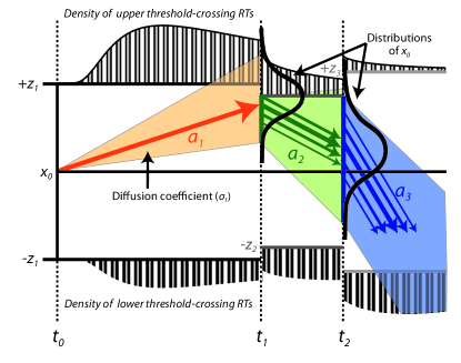
Figure 1: Illustration of the key ideas for computation of FPT properties of the multistage model with piecewise constant drift and thresholds. The distribution of evidence $x(t_{i})$ conditioned on no decision until $t_{i}$ serves as the distribution of initial condition for the $i$-th stage process. If threshold $\zeta_{i+1}<\zeta_{i}$, then probability of instantaneous decision at time $t_{i}$ is computed as the probability of $x(t_{i})$ conditioned on no decision until $t_{i}$ not belonging to the set $(-\zeta_{i},\zeta_{i})$. If threshold $\zeta_{i+1}>\zeta_{i}$, then there is no instantaneous decision and only the support of $x(t_{i})$ conditioned on no decision until $t_{i}$ is increased to $(-\zeta_{i+1},\zeta_{i+1})$.

7 Numerical examples

In this section we apply our calculations from §5 and §6 to a variety of numerical experiments. In doing so, we compare the theoretical predictions obtained from the analysis in this paper with the numerical values obtained through Monte-Carlo simulations, thereby numerically verifying our derivations above. We also provide examples illustrating time pressure or changes in attention over the course of a decision process, and demonstrate how our work can help to find the optimal speed-accuracy trade-off by maximizing reward rate (or any other function of mean first passage time, threshold-hitting probability, and reward). Unless otherwise noted, Monte Carlo simulations were obtained using $1000$ runs; relatively few runs are used so that curves are visually distinguishable. Stochastic simulations use the Euler-Maruyama method with time step size $10^{-3}$. All of the above calculations have been implemented in MATLAB, and all codes used to produce the figures in this section may be found at https://github.com/sffeng/multistage.

7.1 A Four-stage process

Consider a four stage process with drift and diffusion rates given by $(\mu_{1},\mu_{2},\mu_{3},\mu_{4})=(0.1,0.2,0.05,0.3)$ and $(\sigma_{1},\sigma_{2},\sigma_{3},\sigma_{4})=(1,1.5,1.25,2)$, respectively, with $(t_{0},t_{1},t_{2},t_{3})=(0,1,2,3)$ and initial condition $x_{0}=-0.2$. The cumulative distribution function (CDF) of the unconditional and conditional decision time for $\zeta=2$ obtained using the above analytic expressions (solid lines) and Monte-Carlo simulations (dotted lines) is shown in Figure 2(a). Similarly, the unconditional mean decision time, the lower hitting probability, and the mean conditional decision times (for upper/lower responses) are shown in Figure 2(b) as a function of threshold $\zeta$. Note that the analytic expressions match closely with quantities computed using Monte-Carlo simulations. Also, notice that the CDF almost looks like a double-sigmoidal function (it starts to saturate around $0.6$ before picking up and eventually saturating at $1$) due to the drop in drift rate from $0.2$ to $0.05$.

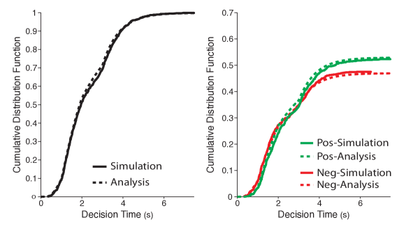
(a) Unconditional and Conditional First Passage Time Distribution

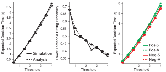
(b) Unconditional Mean Decision Time, Lower Hitting Probability, and Conditional Mean Decision Time

Figure 2: FPT calculations for a four-stage process with drift rates $(\mu_{1},\mu_{2},\mu_{3},\mu_{4})=(0.1,0.2,0.05,0.3)$, diffusion rates $(\sigma_{1},\sigma_{2},\sigma_{3},\sigma_{4})=(1,1.5,1.25,2)$, stage initiation times $(t_{0},t_{1},t_{2},t_{3})=(0,1,2,3)$, and initial condition $x_{0}=-0.2$. The FPT distribution is computed for threshold $\zeta=2$.

7.2 FPT Distribution for a process with Alternating Drift

In this example, the sign of the drift rate changes from stage to stage. This may be used to describe situations in which evidence accumulation changes dynamically with the decision-maker’s focus of attention. For instance, Krajbich et al. (2010) have shown that the process of weighing two value-based options (e.g., foods) can be modeled with a process in which drift rates vary based on the option being attended at any given moment. We consider such a case using a $30$-stage model in which the drift rates $1$ and $-0.75$ alternate (i.e., $\mu_{1}=1$, $\mu_{2}=-0.75$, $\mu_{3}=1$, $\ldots$) to capture a situation in which the decision maker’s attention alternates between two options, one of which has greater perceived value (higher drift rate) than the other. Let $t_{0}=0$ and the remaining $29$ stage initiation times be a fixed realization of $29$ uniformly sampled points between $0$ and $10$. Assume $x_{0}=0$, $\zeta=2$, and let the diffusion rate be stationary and equal to unity ($\sigma_{i}=1$). The unconditional and conditional FPT distributions in this scenario obtained using both the analytic expressions (solid lines) and Monte-Carlo simulations (dotted lines) are shown in Figure 3. Note that the analytic expressions match closely with quantities computed using Monte-Carlo simulations.

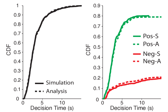
Figure 3: Unconditional and conditional FPT distributions for a $30$-stage model with alternating drift rate. The drift rates are $(\mu_{1},\mu_{2},\mu_{3},\ldots)=(1,-0.75,1,\ldots)$, diffusion rate at each stage is unity, the threshold $\zeta=2$, and stage initiation times are equally spaced throughout the interval $(0,10)$.

7.3 FPT Distribution for a model with gradually time-varying drift

Changes in evidence accumulation may occur gradually over time. For instance, White et al. (2011) proposed a “shrinking spotlight” model of the Eriksen Flanker Task, a task in which participants responding to the direction of a central arrow are influenced by the direction of arrows in the periphery (see also Servan-Schreiber et al., 1990; Liu et al., 2009; Servant et al., 2015). According to these models, evidence accumulation is initially influenced by all of the arrows (central as well as flankers, which may drive an incorrect response, modeled here as as a lower threshold response) but as the attentional spotlight narrows the drift rate is gradually more influenced by the central arrow alone. The multistage model, in spite of having discontinuous changes in parameters, can still be used to approximate a model with gradually time-varying parameters.

As a demonstration, we use a $20$-stage model as an approximation to a model with continuously time-varying drift rate. Assume $\sigma_{i}=1$, $x_{0}=0$, $\zeta=2$, and let the stage initiation times $t_{0},t_{1},\ldots,t_{19}$ be equally spaced throughout the interval $[0,5]$. Furthermore, suppose the drift rate during the $i$-th stage is $-0.2+0.0263(i-1)$. The unconditional and conditional FPT distributions for such a $20$-stage process obtained using the analytic expressions (solid lines) and using Monte-Carlo simulations (dotted lines) are shown in Figure 4. Note that the analytic expressions match closely with quantities computed using Monte-Carlo simulations. We also show the error due to piecewise constant approximation of the drift rate as a function of number of stages (Figure 4, right). It should be noted that even for $5$ stages the approximation error is very small.

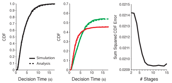
Figure 4: Unconditional (left) and conditional (middle) FPT distributions for a $20$-stage process with gradually increasing drift rate. The drift rate for the $i$-th stage is $\mu_{i}=-0.2+0.0263(i-1)$, diffusion rate at each stage is unity, the threshold $\zeta=2$, and stage initiation times are equally spaced throughout the interval $[0,5]$. Right: The total squared error between the simulated and analytic CDFs (left) decreases with increasing discrete stages of the model. 10,000 simulations were used for each approximation.

7.4 Collapsing Thresholds

One may be interested in modeling a decision process in which thresholds are dynamic rather than constant across stages. This can be used to describe discrete changes in choice strategy, or a continuous change in thresholds over time; the latter approach has been successful at describing behavior under conditions that either involve an explicit response deadline (e.g., Milosavljevic et al., 2010; Frazier and Yu, 2008) or where there is an implicit opportunity cost for longer time spent accumulating evidence (Drugowitsch et al., 2012). Recently, (Voskuilen et al., 2016) used analytic methods to model collapsing boundaries in order to compare fixed boundaries against collapsing boundaries in diffusion models.

Here, we model such a situation using a $20$-stage process, as an approximation to a diffusion model with continuously collapsing thresholds ,i.e., $\zeta\downarrow 0$ with time, the drift rate and the diffusion rate are constant and equal to $0.15$ and $1$, respectively, $x_{0}=0$, and stage initiation times $t_{0},t_{1},\ldots,t_{19}$ are equally spaced throughout the interval $[0,5]$. The threshold in the $i$-th stage is $\zeta_{i}=3-\frac{1}{19}(i-1)$. The unconditional and conditional FPT distributions for such a $20$-stage process obtained using the analytic expressions (solid lines) and using Monte-Carlo simulations (dotted lines) are shown in Figure 5. Note that the analytic expressions match closely with quantities computed using Monte-Carlo simulations.

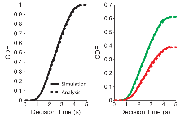
Figure 5: Unconditional and conditional FPT distributions for a $20$-stage process with collapsing thresholds. The drift rate and diffusion rate at each stage are $0.15$ and $1$, respectively. The stage initiation times are equally spaced throughout the interval $[0,5]$, and the threshold at $i$-th stage is $\zeta_{i}=3-\frac{i-1}{19}$, for $i=\{1,\dots,19\}$.

7.5 Optimizing the Speed-Accuracy Trade-off in a Two-stage Model

Human decision-making in many two alternative forced choice signal detection tasks has been successfully captured by the single stage model. In such tasks, hitting the upper/lower boundary is interpreted as a correct/incorrect response. The accuracy of a decision can then be determined by the sign of the drift rate – if $\mu$ is positive, participants are said to be more accurate the more likely they are to hit the upper threshold and more error-prone the more likely they are to hit the lower threshold. One then assumes without loss of generality that the drift rate is positive, in which case the lower hitting probability is called the error rate and the upper hitting probability is called the accuracy. Here, the choice of threshold dictates the speed-accuracy trade-off, i.e., the trade-off between a fast decision and an accurate decision. In the previous examples, the thresholds have been known and we have characterized the associated error rate and first passage time properties. These can be used to define a joint function of speed and accuracy that may dictate how humans/animals choose to set and adjust their threshold. In particular, it has been proposed (Bogacz et al., 2006) that human subjects choose a threshold that maximizes reward rate (RR), defined as

$${\rm RR}=\frac{1-P^{-}}{\mathbb{E}[\tau]+T_{\textup{nd}}},$$ (33)

where $T_{\textup{nd}}$ is the sensory and motor processing time (non-decision time) and $P^{-}$ and $\mathbb{E}[\tau]$ are computed using the expressions derived in §5.

The reward rate for a two-stage process is shown in Figure 6. For the set of parameters in Figure 6, reward rate is maximal at approximately $(\zeta_{1},\zeta_{2})=(0.06,0.01)$. Thus, the maximizing reward rate in this setting interestingly requires that the threshold across stages be different.

Setting the threshold to be constant across stages ($\zeta_{1}=\zeta_{2}$), we can compare how reward rate changes with this constant threshold in a single-stage (traditional) versus a two-stage mode. As shown in Figure 7(a), we find that this reward rate function is unimodal in a single-stage model (as previously observed) whereas it is bimodal in a two-stage model. Figure 7(b) explores this parameter space in greater depth and shows that the curvature of reward rate (and in particular the relative height of its first and second modes) vary as a function of the length and drift rate of the first stage (for example). As a result, this analysis reveals a discontinuous jump in optimal threshold as these parameters vary. Whether individuals are sensitive to these discontinuities when setting thresholds for a multistage decision-making task deserves further exploration.

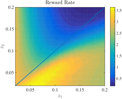
Figure 6: Reward rate as a function of the thresholds for the two-stage model. The parameters are $\mu_{1}=0.5$, $\mu_{2}=-0.1$, $\sigma_{1}=\sigma_{2}=0.1$, $x_{0}=\zeta_{1}/2$, and $t_{1}=0.1$. The non-decision time $T_{\textup{nd}}=0.3$. Note that the maximum reward rate is achieved for $\zeta_{1}\neq\zeta_{2}$.

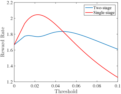
(a) Reward rate for single- and two-stage models

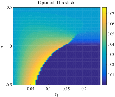
(b) Reward rate for two-stage model

Figure 7: (a) For the single-stage model $\mu_{1}=0.2,\sigma_{1}=0.1$ and $x_{0}=0$, while for the two-stage model $\mu_{1}=0.1$, $\mu_{2}=0.5$, $\sigma_{1}=\sigma_{2}=0.1$, $x_{0}=0$ and $t_{1}=0.15$. The non-decision time $T_{\textup{nd}}=0.3$. The reward rate for the single-stage model is a unimodal function and achieves a unique local maximum, while the reward rate for the two-stage model has two local maxima. (b) Optimal threshold for two-stage model obtained by maximizing reward rate. The left panel shows the variation of the optimal threshold as a function of $t_{1}$ and $\mu_{1}$. The other parameters are $\mu_{2}=0.5$, $\sigma_{1}=\sigma_{2}=0.1$, and $x_{0}=0$. The regions of the contour plot associated with $t_{1}=0$ and $\mu_{1}=0.5$ correspond to the single-stage model.

8 Discussion

In this paper we analyze the first passage time properties of a Wiener process between two absorbing boundaries with piecewise constant (time-dependent) parameters, which we call a multistage model or multistage process. Our main theoretical results, collected in §5, add to previous work on analyzing time-dependent random walk models in psychology and neuroscience. Broadly speaking, these can be split into three approaches. One approach is the integral equation approach introduced and developed in Smith (1995, 2000); Smith and Ratcliff (2009). Another approach is the matrix based Markov Chain approximation which has been applied to a wide variety of multi-attribute choice settings (Diederich and Busemeyer, 2003; Diederich and Oswald, 2016, 2014). A third approach analyzes the backward partial differential equation associated with the multistage process (Ratcliff, 1980; Heath, 1992). The results of §5 align most closely with the work of the third approach, as we also directly analyze the multistage stochastic process, albeit with different techniques. Whereas Ratcliff (1980) and Heath (1992) analyzed a multistage process by solving the Kolmogorov partial differential equation, we employ martingale theory (e.g. the optional sampling theorem) in order to obtain analytic results which extend those of previous studies. In doing so, our work also builds on martingale-based analyses described by Smith (1990) for a single stage model.

The modeler utilizing time-dependent random walk models in decision making should be aware of all of the above approaches, as one approach may demand additional approximations compared to another, due to differences in how they discretize temporal dynamics. For example, when modeling experiments with continuously (gradually) changing stimuli (e.g., White et al. (2011); Zhang et al. (2014)) one may find the integral equation approach more natural, given the continuity and smoothness assumptions built in to the techniques. Diederich and Oswald’s model also allows for continuous changes in boundaries. In contrast, our methods must approximate the underlying gradually changing drift with a piecewise constant function, thereby inducing some additional error in the calculations of first passage times. If, however, the application lends itself well to discrete changes in drift rate or threshold (e.g., Krajbich et al. (2010)), then both the matrix based methods and methods discussed in this paper may be more natural, as they explicitly consider such discrete changes in the underlying calculations. Ornstein-Uhlenbeck processes lend themselves more naturally to the matrix based approach of Diederich and Busemeyer (2003), compared to our analysis in D, since our analysis requires a change in time scale that the matrix method does not. In the specific case of a multistage model (2), our work provides semi-analytic formulas that can be easily computed or studied further (see below). In general, the modeler should be ready to employ the most suitable approach given their situation.

The reader should also be aware of the software tools available for each approach, as there already exist several good non-martingale based software packages for computing FPT statistics. One package implementing the integral equation approach is that of Drugowitsch (2014), which computes first passage time densities using the stable numerical approximations developed in Smith (2000). More recently, highly optimized codes for a broad class of diffusion models have been developed by Verdonck et al. (2015), with implementations on both CPUs and GPUs. Compared to other available codes, Diederich and Busemeyer (2003)’s matrix approach is substantially simpler and more elegant to implement – one can compute desired choice probabilities and mean decision times in less than a few dozen lines of MATLAB code. For practitioners wishing to write all of their own model code from scratch, this may be a considerable advantage. The MATLAB code released with this report provides implementations of the results from §5 and allows one to reproduce all of the figures from §7. Unlike the work of Verdonck et al. (2015), our work is not immediately focused on developing a rapid numerical tool for simulation, but rather on introducing martingale theory as a useful mathematical tool for analyzing multistage decision models. Thus, the codes released with this report are not intended to compete with the efficiency of the aforementioned codes, which have been highly optimized and tuned for throughput, but instead to demonstrate the simplicity and effectiveness of our analysis. These considerations notwithstanding, our results do suggest promising avenues for future numerical work. Particularly relevant is work by Navarro and Fuss (2009); Blurton et al. (2012); Gondan et al. (2014) who developed efficient numerical schemes for evaluating the relevant infinite sums involved in FPT calculations. Similar methods could be applied to results in §5.1 and §5.2 to develop efficient multistage codes, which could in turn contribute to the growing collection of numerical tools available for practitioners using diffusion models to study decision making.

In §3 we re-derived classical mean decision times and choice probabilities equivalent to results first derived for a discrete time random walk model using the Wald identity (Laming, 1968; Link and Heath, 1975; Link, 1975; Smith, 1990), which itself is a corollary of the optional sampling theorem. Smith (1990) notes that results concerning the discrete time random walk model with Gaussian increments and the continuous time single stage Wiener diffusion model of §3 should be equivalent, which is indeed the case. Furthermore, the moment generating function derived in §3.3 is identical to that obtained by (Smith, 1990, p. 9) via the Wald identity. Our aim in presenting §3 was to introduce the martingale analysis used in §5 by first demonstrating its utility in re-deriving these classical results. We hope these calculations provide an intuition for the computations in §5 in a less technical setting. For reviews of the classical results on random walks in psychological decision making, see (Townsend and Ashby, 1983, pp. 300-301) and (Luce, 1986, pp. 328-334).

One particularly useful aspect of equations (20) through (32) is that they demonstrate how various other measures of performance, such as the lower-threshold hitting probability during each stage, evolve as the underlying dynamics change. Using these, one may efficiently compute a variety of behavioral measures of performance without resorting to first computing the FPT densities. Our results may also serve as a starting point for further analysis of more complicated stochastic decision models. In appendix D, we show how our results apply to Ornstein-Uhlenbeck processes, which approximate leaky integration over the course of evidence accumulation, e.g., the Leaky Competing Accumulator model [LCA] (Usher and McClelland, 2001). Given that the LCA itself can in certain cases approximate a reduced form of more complex and biologically plausible models of interactions across neuronal populations (e.g., Wang, 2002; Wong and Wang, 2006; Bogacz, 2007), our work may help analysts better understand time-varying dynamics within and across neural networks, and how such dynamics relate to complex cognitive phenomena.

Beyond its analytic and numerical utility, our uses of martingale theory, and the optional sampling theorem in particular, provide some theoretical insights into random walk decision models. For example, a single stage model with zero drift rate (i.e. Wiener process) and lower/upper thresholds at 0 and 1 necessarily has the qualitative property that the probability of hitting the upper threshold equals the initial (nonrandom) position $x_{0}$. Although these results are known in the probability literature (Doob, 1953), they provide practitioners and experimentalists a unique way of planning and analyzing experiments based on decisions thought to evolve according to diffusion processes. In summary, we hope that the tools described in this article and the results of §5 will encourage computational and mathematical analyses of decision models involving time-dependent parameters.

9 Acknowledgements

We also thank the editor, Philip Smith, and the referees for helpful comments, especially regarding this article’s exposition and discussion. We thank Ryan Webb for the reference to Smith (2000) and the associated code. We thank Phil Holmes and Patrick Simen for helpful comments and discussions. This work was jointly supported by the C.V. Starr Foundation (AS), the Insley-Blair Pyne Fund, ONR grant N00014-14-1-0635 and ARO grant W911NF-14-1-0431(VS and NEL).

10 Bibliography

Appendix A Alternative expression for FPT density of the single stage model

An alternative expression to the FPT density (13) that can be obtained by solving the Fokker-Planck equation (Feller, 1968) is:

$$f(t;x_{0},\theta)=\frac{\pi\sigma^{2}}{4\zeta^{2}}\exp\Big{(}{-\frac{\mu^{2}t}{2\sigma^{2}}}\Big{)}\sum_{n=1}^{+\infty}(-1)^{n-1}n\exp\Big{(}{-\frac{n^{2}\pi^{2}\sigma_{1}^{2}t}{8\zeta^{2}}}\Big{)}\bigg{(}\exp\Big{(}{\frac{\mu(\zeta-x_{0})}{\sigma^{2}}}\Big{)}\sin\Big{(}\frac{n\pi(\zeta+x_{0})}{2\zeta}\Big{)}\\ +\exp\Big{(}{-\frac{\mu(\zeta+x_{0})}{\sigma^{2}}}\Big{)}\sin\Big{(}\frac{n\pi(\zeta-x_{0})}{2\zeta}\Big{)}\bigg{)}.$$

Appendix B Derivation of expressions in §5.1

We first establish (20). First consider the case $\mu_{i}>0$. Let $\{\mathcal{F}_{t}^{i}\}_{t\geq t_{i-1}}$ be the filtration defined by the evolution of the multistage process (2) until time $t$ conditioned on $\tau>t_{i-1}$. A filtration can be thought of as an increasing sequence of available information. For some $s\in(t_{i-1},t)$, as shown in §3, $\{\exp({-2s_{i}x(t)})\}_{t\geq t_{i-1}}$ is a martingale, i.e., $\mathbb{E}[\exp({-2s_{i}x(t)})|\mathcal{F}_{s}^{i}]=\exp({-2s_{i}x(s)})$.

Furthermore, $\hat{\tau}_{i}:=\min\{\tau_{i},t_{i}\}$ is a stopping time. Therefore, it follows from optional sampling theorem that

$$\mathbb{E}[\exp({-2s_{i}X_{i-1}})] =\mathbb{E}[\exp({-2s_{i}x(\hat{\tau}_{i})})]$$

$$=\mathbb{E}[\exp({-2s_{i}x(\tau_{i})})|\tau_{i}\leq t_{i}]\mathbb{P}[\tau_{i}\leq t_{i}]+\mathbb{E}[\exp({-2s_{i}X_{i}})]\mathbb{P}[\tau_{i}>t_{i}]]$$

$$=\big{(}\exp({-2s_{i}\zeta})(1-P^{-}_{i})+\exp({2s_{i}\zeta})P^{-}_{i}\big{)}\mathbb{P}[\tau_{i}\leq t_{i}]+\mathbb{E}[\exp({-2s_{i}X_{i}})]\mathbb{P}[\tau_{i}>t_{i}]].$$

Solving the above equation for $P^{-}_{i}$, we obtain the desired expression.

For $\mu_{i}=0$, , as shown in §3, $\{x(t)\}_{t\geq t_{i}}$ is a martingale. Therefore, applying the optional sampling theorem, we obtain

$$\mathbb{E}[X_{i-1}] =\mathbb{E}[x(\hat{\tau}_{i})]$$

$$=\mathbb{E}[x(\tau_{i})|\tau_{i}\leq t_{i}]\mathbb{P}[\tau_{i}\leq t_{i}]+\mathbb{E}[X_{i}]\mathbb{P}[\tau_{i}>t_{i}]]$$

$$=(1-2P^{-}_{i})\zeta\mathbb{P}[\tau_{i}\leq t_{i}]+\mathbb{E}[X_{i}]\mathbb{P}[\tau_{i}>t_{i}].$$

Solving the above equation for $P^{-}_{i}$, we obtain the desired expression.

The formulas (21) and (22) immediately follow from applying expectation to (14) and (15), respectively.

To establish (23) for $\mu_{i}\neq 0$, we note from §3 that for the $i$-th stage, $\{x(t)-\mu_{i}t\}_{t\geq t_{i}}$ is a martingale. Therefore, applying the optional sampling theorem, we obtain

$$\mathbb{E}[X_{i-1}]-\mu_{i}t_{i-1} =\mathbb{E}[x(\hat{\tau}_{i})-\mu_{i}\hat{\tau}_{i}]$$

$$=\mathbb{E}[x(\tau_{i})-\mu_{i}\tau_{i}|\tau_{i}\leq t_{i}]\mathbb{P}[\tau_{i}\leq t_{i}]+\mathbb{E}[(X_{i}-\mu_{i}t_{i}]\mathbb{P}[\tau_{i}>t_{i}]$$

$$=\big{(}\zeta(1-P^{-}_{i})-\zeta P^{-}_{i}-\mu_{i}\mathbb{E}[\tau_{i}|\tau_{i}\leq t_{i}]\big{)}\mathbb{P}[\tau_{i}\leq t_{i}]+(\mathbb{E}[X_{i}]-\mu_{i}t_{i})\mathbb{P}[\tau_{i}>t_{i}].$$

Solving the above equation for $\mathbb{E}[\tau_{i}|\tau_{i}\leq t_{i}]$ yields the desired expression.

For $\mu_{i}=0$, we note from §3 that $\{x(t)^{2}-\sigma_{i}^{2}t\}_{t\geq t_{i-1}}$ is a martingale. Therefore, applying the optional sampling theorem, we obtain

$$\mathbb{E}[X_{i}^{2}]-\sigma_{i}^{2}t_{i-1} =\mathbb{E}[x(\hat{\tau})^{2}-\sigma_{i}^{2}\hat{\tau}_{i}]$$

$$=\mathbb{E}[x(\tau_{i})^{2}-\sigma_{i}^{2}\tau_{i}|\tau_{i}\leq t_{i}]\mathbb{P}[\tau_{i}\leq t_{i}]+\mathbb{E}[X_{i}^{2}-\sigma_{i}^{2}t_{i}]\mathbb{P}[\tau_{i}>t_{i}]]$$

$$=(\zeta^{2}-\sigma_{i}^{2}\mathbb{E}[\tau_{i}|\tau_{i}\leq t_{i}])\mathbb{P}[\tau_{i}\leq t_{i}]+(\mathbb{E}[X_{i}^{2}]-\sigma_{i}^{2}t_{i})\mathbb{P}[\tau_{i}>t_{i}].$$

Solving the above equation for $\mathbb{E}[\tau_{i}|\tau_{i}\leq t_{i}]$ yields the desired expression.

Next, we need to establish that the Laplace transform of the density for the FPT for a particular decision made before $t_{i}$ is

$$\mathbb{E}[\exp({-\alpha\tau_{i}})\boldsymbol{1}(x(\tau_{i})=\zeta|\tau_{i}\leq t_{i})]\\ =\frac{\exp({-\alpha t_{i-1}})\mathbb{E}[T^{\textup{mgf}}_{+}(\mu_{i},\sigma_{i},\zeta,X_{i-1},\alpha)]-\exp({-\alpha t_{i}})\mathbb{E}[T^{\textup{mgf}}_{+}(\mu_{i},\sigma_{i},\zeta,X_{i},\alpha)]\mathbb{P}[\tau_{i}>t_{i}]]}{\mathbb{P}[\tau_{i}\leq t_{i}]},$$

$$\mathbb{E}[\exp({-\alpha\tau_{i}})\boldsymbol{1}(x(\tau_{i})=-\zeta|\tau_{i}\leq t_{i})]\\ =\frac{\exp({-\alpha t_{i-1}})\mathbb{E}[T^{\textup{mgf}}_{-}(\mu_{i},\sigma_{i},\zeta,X_{i-1},\alpha)]-\exp({-\alpha t_{i}})\mathbb{E}[T^{\textup{mgf}}_{-}(\mu_{i},\sigma_{i},\zeta,X_{i},\alpha)\mathbb{P}[\tau_{i}>t_{i}]]}{\mathbb{P}[\tau_{i}\leq t_{i}]}.$$

To establish this, we consider the stochastic process $\exp({\lambda x(t)-\lambda\mu_{i}t-\lambda^{2}\sigma^{2}_{i}t/2})$. From §3, we note that $\{\exp({\lambda x(t)-\lambda\mu_{i}t-\lambda^{2}\sigma^{2}_{i}t/2})\}_{t\geq t_{i-1}}$ is a martingale for each $\lambda\in\mathbb{R}$, i.e.,

$$\mathbb{E}[\exp({\lambda x(t)-\lambda\mu_{i}t-\lambda^{2}\sigma^{2}_{i}t/2})|\mathcal{F}_{s}^{i}]=\exp({\lambda x(s)-\lambda\mu_{i}s-\lambda^{2}\sigma_{i}^{2}s/2}).$$

We choose two particular values of $\lambda$:

$$\lambda_{1}=\frac{-\mu_{i}-\sqrt{\mu_{i}^{2}+2\alpha\sigma_{i}^{2}}}{\sigma_{i}^{2}},\quad\text{and}\quad\lambda_{2}=\frac{-\mu_{i}+\sqrt{\mu_{i}^{2}+2\alpha\sigma_{i}^{2}}}{\sigma_{i}^{2}}.$$

Note that for $\lambda\in\{\lambda_{1},\lambda_{2}\}$, $\lambda\mu_{i}t+\lambda^{2}\sigma^{2}_{i}t/2=\alpha$. Therefore, stochastic processes $\{\exp({\lambda_{1}x(t)-\alpha t})\}_{t\geq 0}$ and $\{\exp({\lambda_{2}x(t)-\alpha t})\}_{t\geq t_{i-1}}$ are martingales. Now applying the optional sampling theorem, we obtain

$$\mathbb{E}[\exp({\lambda_{1}X_{i-1}-\alpha t_{i-1}})]=\mathbb{E}[\exp({\lambda_{1}x(\hat{\tau})-\alpha\hat{\tau}})]=\exp({\lambda_{1}\zeta})\mathbb{E}[\exp({-\alpha\tau_{i}})\boldsymbol{1}(x(\tau_{i})=\zeta\;\&\;\tau_{i}\leq t_{i})]\\ +\exp({-\lambda_{1}\zeta})\mathbb{E}[\exp({-\alpha\tau})\boldsymbol{1}(x(\tau_{i})=-\zeta\;\&\;\tau_{i}\leq t_{i})]+\exp({-\alpha t_{i}})\mathbb{E}[\exp({\lambda_{1}X_{i}})]\mathbb{P}[\tau_{i}>t_{i}].$$ (34)

Similarly,

$$\mathbb{E}[\exp({\lambda_{2}X_{i-1}-\alpha t_{i-1}})]=\exp({\lambda_{2}\zeta})\mathbb{E}[\exp({-\alpha\tau_{i}})\boldsymbol{1}(x(\tau)=\zeta\;\&\;\tau_{i}\leq t_{i})]\\ +\exp({-\lambda_{2}\zeta})\mathbb{E}[\exp({-\alpha\tau_{i}})\boldsymbol{1}(x(\tau)=-\zeta\;\&\;\tau_{i}\leq t_{i})]+\exp({-\alpha t_{i}})\mathbb{E}[\exp({\lambda_{2}X_{i}})]\mathbb{P}[\tau_{i}>t_{i}]].$$ (35)

Equations (34) and (35) are two simultaneous equations in two unknowns $\mathbb{E}[\exp({-\alpha\tau_{i}})\boldsymbol{1}(x(\tau_{i})=\zeta\;\&\;\tau_{i}\leq t_{i})]$ and $\mathbb{E}[\exp({-\alpha\tau_{i}})\boldsymbol{1}(x(\tau_{i})=-\zeta\;\&\;\tau_{i}\leq t_{i})]$. Solving for these unknowns, we obtain

$$\mathbb{E}[\exp({-\alpha\tau_{i}})\boldsymbol{1}(x(\tau_{i})=\zeta\;\&\;\tau_{i}\leq t_{i})]=\frac{1}{\exp({2\lambda_{1}\zeta})-\exp({2\lambda_{2}\zeta})}\bigg{(}\exp({-\alpha t_{i-1}})\mathbb{E}[\exp({\lambda_{1}(X_{i-1}+\zeta)})\\ -\exp({\lambda_{2}(X_{i-1}+\zeta)})]-\exp({-\alpha t_{i}})\mathbb{E}[\exp({\lambda_{1}(X_{i}+\zeta)})-\exp({\lambda_{2}(X_{i}+\zeta)})]\mathbb{P}[\tau_{i}>t_{i}]\bigg{)},$$

and

$$\mathbb{E}[\exp({-\alpha\tau_{i}})\boldsymbol{1}(x(\tau_{i})=-\zeta\;\&\;\tau_{i}\leq t_{i})]=\frac{1}{\exp({-2\lambda_{1}\zeta})-\exp({-2\lambda_{2}\zeta})}\bigg{(}\exp({-\alpha t_{i-1}})\mathbb{E}[\exp({-\lambda_{1}(\zeta-X_{i-1})})\\ -\exp({-\lambda_{2}(\zeta-X_{i-1})})]-\exp({-\alpha t_{i}})\mathbb{E}[(\exp({-\lambda_{1}(\zeta-X_{i})})-\exp({-\lambda_{2}(\zeta-X_{i})}))]\mathbb{P}[\tau_{i}>t_{i}]\bigg{)}.$$

Simplifying these expressions, we obtain the desired expression.

Finally, (24) and (iv) follow from differentiating the Laplace transform with respect to $-\alpha$, and then evaluating at $\alpha=0$.

Appendix C Performance metrics for the overall multistage process

We start by establishing (26). Since $t\in(t_{k-1},t_{k}]$,

$$\mathbb{P}[\tau\leq t] =\mathbb{P}[\tau\leq t\;\&\;\tau\leq t_{k-1}]+\mathbb{P}[\tau\leq t\;\&\;\tau>t_{k-1}]$$

$$=\mathbb{P}[\tau\leq t_{k-1}]+\mathbb{P}[\tau\leq t|\tau>t_{k-1}]\mathbb{P}[\tau>t_{k-1}]$$

$$=1-\prod_{i=1}^{k-1}\mathbb{P}[\tau>t_{i}|\tau>t_{i-1}]+\mathbb{P}[\tau_{k}\leq t]\prod_{i=1}^{k-1}\mathbb{P}[\tau>t_{i}|\tau>t_{i-1}]$$

$$=1-\prod_{i=1}^{k-1}\mathbb{P}[\tau_{i}>t_{i}]+\mathbb{P}[\tau_{k}\leq t]\prod_{i=1}^{k-1}\mathbb{P}[\tau_{i}>t_{i}].$$

We now establish (27). We note that

$$\mathbb{E}[\tau] =\sum_{i=1}^{n}\mathbb{E}[\tau\boldsymbol{1}(t_{i-1}<\tau\leq t_{i})]$$

$$=\sum_{i=1}^{n}\mathbb{E}[\tau\boldsymbol{1}(\tau\leq t_{i})|\tau>t_{i-1}]\mathbb{P}[\tau>t_{i-1}]$$

$$=\sum_{i=1}^{n}\Big{(}\mathbb{E}[\tau_{i}|\tau_{i}\leq t_{i}]\mathbb{P}[\tau_{i}\leq t_{i}]\prod_{j=1}^{i-1}\mathbb{P}[\tau_{j}>t_{j}]\Big{)}.$$

To establish (28), we note that

$$P^{-} =\sum_{i=1}^{n+1}\mathbb{P}(x(\tau)=-\zeta\text{ and }t_{i-1}\leq\tau<t_{i})$$

$$=\sum_{i=1}^{n+1}\mathbb{P}(x(\tau)-\zeta\text{ and }\tau<t_{i}|\tau>t_{i-1})\mathbb{P}[\tau>t_{i-1}]$$

$$=\sum_{i=1}^{n}\Big{(}P^{-}_{i}\mathbb{P}[\tau_{i}<t_{i}]\prod_{j=1}^{i-1}\mathbb{P}[\tau_{j}>t_{j}]\Big{)}.$$

Equations (29) and (30) follow similarly to (27), and Equations (31) and (32) follow similarly to (26).

Appendix D Time-varying Ornstein-Uhlenbeck model

In this section, we discuss how the ideas presented in §5 and §6 can be used to computed FPT properties for a time varying Ornstein-Uhlenbeck (O-U) model.

The O-U model captures decision-making through the first passage of trajectories of an O-U process (Cox and Miller, 1965) through two thresholds. Our calculations for the multistage process also help analyze the Ornstein-Uhlenbeck (O-U) model. Similar to the multistage process, the $n$-stage O-U process with piecewise constant parameters is defined by

$$dx(t)=\mu(t)dt-\lambda(t)x(t)dt+\sigma(t)dW(t),\quad x(t_{0})=x_{0},$$ (36)

where

$$\mu(t) =\mu_{i},\quad\text{for }t_{i-1}\leq t<t_{i},$$

$$\sigma(t) =\sigma_{i},\quad\text{for }t_{i-1}\leq t<t_{i},$$

$$\lambda(t) =\lambda_{i},\quad\text{for }t_{i-1}\leq t<t_{i},$$

for each $i\in\{1,\dots,n\}$. Due to the extra $-\lambda(t)x(t)dt$ term, the O-U process is a leaky integrator, while the original single stage process is a perfect integrator ($\lambda(t)=0$).

Here, leaky integration means that as the noisy signal is integrated in time with exponentially increasing ($\lambda<0$) or decreasing ($\lambda>0)$ weights on past observations. Such exponential weights lead to ‘recency’ or ‘decay’ effects, i.e., the earlier stages (or late stages) may have greater influence on the ultimate decision, whereas with the single stage process, all of the signal throughout the entire decision period is weighed equally.

D.1 The O-U process as a transformation of the Wiener process

In this section we show how our calculations for the multistage process can be easily applied to decision models driven by O-U processes via a transformed Wiener process (Cox and Miller, 1965, §5.9).

Consider the single-stage O-U process

$$dx(t)=\mu dt-\lambda x(t)dt+\sigma dW(t),\;x(t_{0})=x_{0}.$$ (37)

The O-U process (37) can be written as a time-varying location-scale transformation of the Wiener process (Cox and Miller, 1965, §5.9), i.e.,

$$x(t)=\frac{\mu}{\lambda}(1-\exp({-\lambda t}))+\exp({-\lambda t})x_{0}+\exp({-\lambda t})W\Big{(}\frac{\sigma^{2}(\exp({2\lambda t})-1)}{2\lambda}\Big{)}.$$ (38)

In order to derive (38), note that for O-U process (37)

$$x(t)=x(0)\exp(-\lambda t)+\frac{\mu}{\lambda}(1-\exp(-\lambda t))+\sigma\int_{0}^{t}\exp(-\lambda s)dW(s),$$

Note that the stochastic process $\sigma\int_{0}^{t}\exp(-\lambda s)dW(s)$ is equivalent to the stochastic process $\sigma W((1-\exp(-2\lambda t))/2\lambda)$ in the sense of distribution. Furthermore, $\sigma W((1-\exp(-2\lambda t))/2\lambda)$ is equivalent to the stochastic process $e^{-\lambda t}W(\sigma^{2}(\exp(2\lambda t)-1)/2\lambda)$ in a similar sense. This means that for each realization of the process $\sigma\int_{0}^{t}\exp(-\lambda s)dW(s)$ there exists an identical realization of the process $e^{-\lambda t}W(\sigma^{2}(\exp(2\lambda t)-1)/2\lambda)$.

If we define the transformed time by $u(t):=\frac{\sigma^{2}(\exp({2\lambda t})-1)}{2\lambda}$ so that $t=\frac{1}{2\lambda_{1}}\log(1+\frac{2\lambda u}{\sigma^{2}})$. Then

$$x_{0}+W(u(t))=\Big{(}x(t)-\frac{\mu}{\lambda}\Big{)}\exp({\lambda t})+\frac{\mu}{\lambda}=\Big{(}x(t)-\frac{\mu}{\lambda}\Big{)}\sqrt{1+\frac{2\lambda u(t)}{\sigma^{2}}}+\frac{\mu}{\lambda}.$$

We refer to this process as a Wiener process evolving on exponential time scale.

D.2 First passage time of the O-U process

We now consider the first passage time of the O-U process (37) with respect to symmetric thresholds $\pm\zeta$. If $x(t)=\pm\zeta$, we have $x_{0}+W(u)=\big{(}\pm\zeta-\frac{\mu}{\lambda}\big{)}\sqrt{1+\frac{2\lambda u}{\sigma^{2}}}+\frac{\mu}{\lambda}$. We denote this last quantity by $\zeta^{\pm}(u)$. Consequently, the FPT for $x(t)$ with respect to thresholds $\pm\zeta$ is a continuous transformation of the FPT of a Wiener process starting at $x_{0}$ and evolving on the transformed time $u$ with respect to time-varying thresholds at $\zeta^{\pm}(u)$. Since $u$ is a monotonically increasing function, the distribution of the first passage time $\tau$ can be obtained from $u(\tau)$, the FPT distribution of the Wiener process. Furthermore, the lower threshold hitting probabilities of the two processes are the same.

Note that in transforming the FPT problem for the O-U process (37) to the FPT problem for the Wiener process evolving on exponential time scale, removes all the parameters from the underlying process $x_{0}+W(u)$ and puts them in thresholds $\zeta^{\pm}(u)$ and exponential time scale $u$. In addition to utilizing the results of §5 to multistage O-U processes, the above transformation is also helpful is speeding up Monte-Carlo simulations of the O-U process. Since the transformed process evolves on exponential time scale, the Monte-Carlo simulations with transformed process should roughly take time that is a logarithmic function of time taken by the O-U process (37).

Computation of FPT distributions for the Wiener process with time-varying thresholds is, to our knowledge, not analytically tractable. However, the time-varying thresholds can be approximated by piecewise constant time-varying thresholds and approximate FPT distributions can be computed using the multistage model. While the thresholds $\zeta^{\pm}$ are asymmetric for the transformed process (i.e. $\zeta^{+}\neq-\zeta^{-}$), unlike in the case described for the multistage process; such a case can be easily handled by replacing the expression in (13) and (18) with corresponding expressions for asymmetric thresholds (see Douady, 1999; Borodin and Salminen, 2002).

D.3 Approximate computation of the FPT distribution of the multistage O-U process

Similar to the transformation described in D.1, the multistage O-U process (36) for $t\in[t_{i-1},t_{i})$ can be written as

$$x(t)=\frac{\mu_{i}}{\lambda_{i}}(1-\exp({-\lambda_{i}(t-t_{i-1})}))+\exp({-\lambda_{i}(t-t_{i-1})})x(t_{i-1})\\ +\exp({-\lambda_{i}(t-t_{i-1})})W\Big{(}\frac{\sigma_{i}^{2}(\exp({2\lambda_{i}(t-t_{i-1})})-1)}{2\lambda_{i}}\Big{)}.$$ (39)

Let $u_{i}(t)={\sigma_{i}^{2}(\exp({2\lambda_{i}(t-t_{i-1})})-1)}/{2\lambda_{i}}$. Also, let $\tau_{i}$ and $X_{i-1}$, $i\in\{1,\dots,n\}$ be defined similarly to the multistage model. Then, conditioned on a realization of $X_{i-1}$, the FPT problem of the $i$-th stage O-U process can be equivalently written as the FPT problem of the Wiener process $X_{i-1}+W(u_{i}(t))$ with respect to thresholds

$$\zeta_{i}^{\pm}(u_{i}(t))=\Big{(}\pm\zeta-\frac{\mu_{i}}{\lambda_{i}}\Big{)}\sqrt{1+\frac{2\lambda_{i}u_{i}(t)}{\sigma_{i}^{2}}}+\frac{\mu_{i}}{\lambda_{i}}.$$

We can approximate each stage of the O-U process (36) by a multistage process representing the above Wiener process with time varying thresholds. This sequence of multistage processes is itself a larger multistage process that approximates (36) and its FPT distribution can be computed using the method developed in §5. Note that this method only yields FPT distributions. The expected decision times and probability of hitting a particular threshold can be computed by integrating these distributions.

References

• Blurton et al. (2012) Blurton, S. P., Kesselmeier, M., Gondan, M., 2012. Fast and accurate calculations for cumulative first-passage time distributions in Wiener diffusion models. Journal of Mathematical Psychology 56 (6), 470–475.
• Bogacz (2007) Bogacz, R., 2007. Optimal decision-making theories: linking neurobiology with behaviour. Trends in Cognitive Sciences 11 (3), 118–125.
• Bogacz et al. (2006) Bogacz, R., Brown, E., Moehlis, J., Holmes, P. J., Cohen, J. D., 2006. The physics of optimal decision making: A formal analysis of models of performance in two-alternative forced-choice tasks. Psychological Review 113 (4), 700–765.
• Borodin and Salminen (2002) Borodin, A. N., Salminen, P., 2002. Handbook of Brownian Motion: Facts and Formulae. Springer.
• Brunton et al. (2013) Brunton, B. W., Botvinick, M. M., Brody, C. D., 2013. Rats and humans can optimally accumulate evidence for decision-making. Science 340 (6128), 95–98.
• Busemeyer and Diederich (2010) Busemeyer, J. R., Diederich, A., 2010. Cognitive modeling. Sage.
• Cisek et al. (2009) Cisek, P., Puskas, G. A., El-Murr, S., 2009. Decisions in changing conditions: The urgency-gating model. The Journal of Neuroscience 29 (37), 11560–11571.
• Cox and Miller (1965) Cox, D. R., Miller, H. D., 1965. The Theory of Stochastic Processes. Methuen & Co. Ltd.
• Diederich and Busemeyer (2003) Diederich, A., Busemeyer, J. R., 2003. Simple matrix methods for analyzing diffusion models of choice probability, choice response time, and simple response time. Journal of Mathematical Psychology 47 (3), 304 – 322.
• Diederich and Busemeyer (2006) Diederich, A., Busemeyer, J. R., 2006. Modeling the effects of payoff on response bias in a perceptual discrimination task: Bound-change, drift-rate-change, or two-stage-processing hypothesis. Perception & Psychophysics 68 (2), 194–207.
URL http://dx.doi.org/10.3758/BF03193669
• Diederich and Oswald (2014) Diederich, A., Oswald, P., 2014. Sequential sampling model for multiattribute choice alternatives with random attention time and processing order. Frontiers in Human Neuroscience 8 (697), 1–13.
• Diederich and Oswald (2016) Diederich, A., Oswald, P., 2016. Multi-stage sequential sampling models with finite or infinite time horizon and variable boundaries. Journal of Mathematical Psychology. In press.
• Doob (1953) Doob, J.-L., 1953. Stochastic Processes. John Wiley & Sons, Inc., Chapman & Hall.
• Douady (1999) Douady, R., 1999. Closed form formulas for exotic options and their lifetime distribution. International Journal of Theoretical and Applied Finance 2 (1), 17–42.
• Drugowitsch (2014) Drugowitsch, J., 2014. C++ diffusion model toolset with Python and Matlab interfaces. GitHub repository: https://github.com/jdrugo/dm, commit: 5729cd891b6ab37981ffacc02d04016870f0a998.
• Drugowitsch et al. (2012) Drugowitsch, J., Moreno-Bote, R., Churchland, A. K., Shadlen, M. N., Pouget, A., 2012. The cost of accumulating evidence in perceptual decision making. The Journal of Neuroscience 32 (11), 3612–3628.
• Durrett (2010) Durrett, R., 2010. Probability: Theory and Examples. Cambridge University Press.
• Farkas and Fulop (2001) Farkas, Z., Fulop, T., 2001. One-dimensional drift-diffusion between two absorbing boundaries: Application to granular segregation. Journal of Physics A: Mathematical and General 34 (15), 3191–3198.
• Feller (1968) Feller, W., 1968. An Introduction to Probability Theory and its Applications. Vol. 1. John Wiley & Sons.
• Feng et al. (2009) Feng, S., Holmes, P., Rorie, A., Newsome, W. T., 2009. Can monkeys choose optimally when faced with noisy stimuli and unequal rewards. PLoS Computational Biology 5 (2), e1000284.
• Frazier and Yu (2008) Frazier, P., Yu, A. J., 2008. Sequential hypothesis testing under stochastic deadlines. In: Platt, J., Koller, D., Singer, Y., Roweis, S. (Eds.), Advances in Neural Information Processing Systems 20. Curran Associates, Inc., pp. 465–472.
• Gold and Shadlen (2001) Gold, J. I., Shadlen, M. N., 2001. Neural computations that underlie decisions about sensory stimuli. Trends in Cognitive Sciences 5 (1), 10–16.
• Gold and Shadlen (2007) Gold, J. I., Shadlen, M. N., 2007. The neural basis of decision making. Annual Review of Neuroscience 30 (1), 535–574.
• Gondan et al. (2014) Gondan, M., Blurton, S. P., Kesselmeier, M., Jun. 2014. Even faster and even more accurate first-passage time densities and distributions for the Wiener diffusion model. Journal of Mathematical Psychology 60, 20–22.
• Heath (1992) Heath, R. A., 1992. A general nonstationary diffusion model for two-choice decision-making. Mathematical Social Sciences 23 (3), 283–309.
• Horrocks and Thompson (2004) Horrocks, J., Thompson, M. E., 2004. Modeling event times with multiple outcomes using the Wiener process with drift. Lifetime Data Analysis 10 (1), 29–49.
• Hubner et al. (2010) Hubner, R., Steinhauser, M., Lehle, C., 2010. A dual-stage two-phase model of selective attention. Psychological Review 117 (3), 759–784.
• Karatzas and Shreve (1998) Karatzas, I., Shreve, S., 1998. Brownian Motion and Stochastic Calculus, 2nd Edition. Vol. 113. Springer-Verlag New York.
• Krajbich et al. (2010) Krajbich, I., Armel, C., Rangel, A., 2010. Visual fixations and the computation and comparison of value in simple choice. Nature Neuroscience 13 (10), 1292–1298.
• Laming (1968) Laming, D. R. J., 1968. Information theory of choice-reaction times. Academic Press.
• Lin (1998) Lin, X. S., 1998. Double barrier hitting time distributions with applications to exotic options. Insurance: Mathematics and Economics 23 (1), 45–58.
• Link and Heath (1975) Link, S., Heath, R., 1975. A sequential theory of psychological discrimination. Psychometrika 40 (1), 77–105.
• Link (1975) Link, S. W., 1975. The relative judgment theory of two choice response time. Journal of Mathematical Psychology 12 (1), 114–135.
• Liu et al. (2009) Liu, S., Yu, A. J., Holmes, P., 2009. Dynamical analysis of Bayesian inference models for the Eriksen task. Neural Computation 21 (6), 1520–1553.
• Luce (1986) Luce, R. D., 1986. Response times: Their role in inferring elementary mental organization. No. 8. Oxford University Press.
• Milosavljevic et al. (2010) Milosavljevic, M., Malmaud, J., Huth, A., Koch, C., Rangel, A., 2010. The drift diffusion model can account for the accuracy and reaction time of value-based choices under high and low time pressure. Judgment and Decision Making 5 (6), 437–449.
• Mormann et al. (2010) Mormann, M. M., Malmaud, J., Huth, A., Koch, C., Rangel, A., 2010. The drift diffusion model can account for the accuracy and reaction time of value-based choices under high and low time pressure. Available at SSRN 1901533.
• Navarro and Fuss (2009) Navarro, D. J., Fuss, I. G., 2009. Fast and accurate calculations for first-passage times in Wiener diffusion models. Journal of Mathematical Psychology 53 (4), 222–230.
• Ratcliff (1978) Ratcliff, R., 1978. A theory of memory retrieval. Psychological Review 85 (2), 59–108.
• Ratcliff (1980) Ratcliff, R., 1980. A note on modeling accumulation of information when the rate of accumulation changes over time. Journal of Mathematical Psychology 21 (2), 178–184.
• Ratcliff and McKoon (2008) Ratcliff, R., McKoon, G., 2008. The diffusion decision model: Theory and data for two-choice decision tasks. Neural Computation 20 (4), 873 – 922.
• Ratcliff and Rouder (1998) Ratcliff, R., Rouder, J. N., 1998. Modeling response times for two-choice decisions. Psychological Science 9 (5), 347–356.
• Ratcliff and Smith (2004) Ratcliff, R., Smith, P. L., 2004. A comparison of sequential sampling models for two-choice reaction time. Psychological Review 111 (2), 333–367.
• Ratcliff et al. (2016) Ratcliff, R., Smith, P. L., Brown, S. D., McKoon, G., 2016. Diffusion decision model: Current issues and history. Trends in Cognitive Sciences 20 (4), 260–281.
• Revuz and Yor (1999) Revuz, D., Yor, M., 1999. Continuous Martingales and Brownian Motion. Vol. 293. Springer Berlin Heidelberg.
• Servan-Schreiber et al. (1990) Servan-Schreiber, D., Printz, H., Cohen, J., 1990. A network model of catecholamine effects- gain, signal-to-noise ratio, and behavior. Science 249 (4971), 892–895.
• Servant et al. (2015) Servant, M., White, C., Montagnini, A., Burle, B., 2015. Using covert response activation to test latent assumptions of formal decision-making models in humans. The Journal of Neuroscience 35 (28), 10371–10385.
• Shadlen and Newsome (2001) Shadlen, M. N., Newsome, W. T., 2001. Neural basis of a perceptual decision in the parietal cortex (area LIP) of the rhesus monkey. Journal of Neurophysiology 86 (4), 1916–1936.
• Simen et al. (2009) Simen, P., Contreras, D., Buck, C., Hu, P., Holmes, P., Cohen, J. D., 2009. Reward rate optimization in two-alternative decision making: Empirical tests of theoretical predictions. Journal of Experimental Psychology: Human Perception and Performance 35 (6), 1865.
• Smith (1990) Smith, P. L., 1990. A note on the distribution of response times for a random walk with Gaussian increments. Journal of Mathematical Psychology 34 (4), 445–459.
• Smith (1995) Smith, P. L., 1995. Psychophysically principled models of visual simple reaction time. Psychological review 102 (3), 567.
• Smith (2000) Smith, P. L., 2000. Stochastic dynamic models of response time and accuracy: A foundational primer. Journal of Mathematical Psychology 44 (3), 408 – 463.
• Smith and Ratcliff (2009) Smith, P. L., Ratcliff, R., 2009. An integrated theory of attention and decision making in visual signal detection. Psychological review 116 (2), 283.
• Srivastava et al. (2016) Srivastava, V., Holmes, P., Simen, P., 2016. Explicit moments of decision times for single- and double-threshold drift-diffusion processes. Journal of Mathematical Psychology.  In press.
• Townsend and Ashby (1983) Townsend, J. T., Ashby, F. G., 1983. Stochastic modeling of elementary psychological processes. Cambridge University Press.
• Usher and McClelland (2001) Usher, M., McClelland, J., 2001. The time course of perceptual choice: the leaky, competing accumulator model. Psychological Review 108 (3), 550.
• Verdonck et al. (2015) Verdonck, S., Meers, K., Tuerlinckx, F., 2015. Efficient simulation of diffusion-based choice rt models on CPU and GPU. Behavior Research Methods, 1–15.
• Voskuilen et al. (2016) Voskuilen, C., Ratcliff, R., Smith, P. L., 2016. Comparing fixed and collapsing boundary versions of the diffusion model. Journal of Mathematical Psychology 73, 59–79.
• Wagenmakers et al. (2007) Wagenmakers, E.-J., Van Der Maas, H. L., Grasman, R. P., 2007. An EZ-diffusion model for response time and accuracy. Psychonomic Bulletin & Review 14 (1), 3–22.
• Wang (2002) Wang, X.-J., 2002. Probabilistic decision making by slow reverberation in cortical circuits. Neuron 36 (5), 955–968.
• Webb (2015) Webb, R., Jul. 2015. The dynamics of stochastic choice. Working paper: available at SSRN 2226018.
• White et al. (2011) White, C. N., Ratcliff, R., Starns, J. J., 2011. Diffusion models of the flanker task: Dzhaniscrete versus gradual attentional selection. Cognitive Psychology 63 (4), 210–238.
• Wong and Wang (2006) Wong, K.-F., Wang, X.-J., 2006. A recurrent network mechanism of time integration in perceptual decisions. The Journal of Neuroscience 26 (4), 1314–1328.
• Zhang et al. (2014) Zhang, S., Lee, M. D., Vandekerckhove, J., Maris, G., Wagenmakers, E.-J., 2014. Time-varying boundaries for diffusion models of decision making and response time. Frontiers in Psychology 5 (1364).