Non-self-averaging in Ising spin glasses; hyperuniversality

Abstract

Ising spin glasses with bimodal and Gaussian near-neighbor interaction distributions are studied through numerical simulations. The non-self-averaging (normalized inter-sample variance) parameter $U_{22}(T,L)$ for the spin glass susceptibility (and for higher moments $U_{nn}(T,L)$) is reported for dimensions $2,3,4,5$ and $7$. In each dimension $d$ the non-self-averaging parameters in the paramagnetic regime vary with the sample size $L$ and the correlation length $\xi(T,L)$ as $U_{nn}(\beta,L)=[K_{d}\xi(T,L)/L]^{d}$, and so follow a renormalization group law due to Aharony and Harris aharony:96 . Empirically, it is found that the $K_{d}$ values are independent of $d$ to within the statistics. The maximum values $[U_{nn}(T,L)]_{\max}$ are almost independent of $L$ in each dimension, and remarkably the estimated thermodynamic limit critical $[U_{nn}(T,L)]_{\max}$ peak values are also dimension-independent to within the statistics and so are ”hyperuniversal”. These results show that the form of the spin-spin correlation function distribution at criticality in the large $L$ limit is independent of dimension within the ISG family. Inspection of published non-self-averaging data for $3$D Heisenberg and XY spin glasses the light of the Ising spin glass non-self-averaging results show behavior incompatible with a spin-driven ordering scenario, but compatible with that expected on a chiral-driven ordering interpretation.

I Introduction

The non-self-averaging parameter, usually noted $A$ or $U_{22}$, represents the normalized inter-sample variability for systems such as diluted ferromagnets or spin glasses where the microscopic structures of the interactions within individual samples are not identical. The parameter is defined for ferromagnets as the inter-sample variance of the susceptibility normalized by the mean susceptibility squared aharony:96 ,

$$U_{22}(\beta,L)=\left(\frac{\sigma_{\chi}(T,L)}{\chi(T,L)}\right)^{2}=\frac{\mathrm{var}\!\left(\left\langle q^{2}\right\rangle\right)}{\left[\left\langle q^{2}\right\rangle\right]^{2}}$$ (1)

where $\sigma(T,L)$ is the standard deviation of the equilibrium sample-by-sample distribution of the susceptibility. We denote by $\left\langle\cdots\right\rangle$ the thermal mean for a single sample and by $\left[\cdots\right]$ the sample mean. In ISGs the spin glass susceptibility replaces $\chi$. The non-self-averaging definition can be widened to other observables aharony:96 ; we will also discuss the behavior of non-self-averging of higher moments $\left\langle q^{3}\right\rangle$ and $\left\langle q^{4}\right\rangle$ of of the spin-spin correlation $q$.

Aharony and Harris aharony:96 gave a fundamental renormalization group discussion of non-self-averaging in diluted ferromagnets, which can be applied also to spin glass models. First, they showed that in the paramagnetic regime, at temperatures above the critical temperature, $U_{22}$ (which they referred to as $R_{\chi}$) behaves as

$$U_{22}(T,L)\sim(\xi(T,L)/L)^{d}$$ (2)

where $d$ is the dimension of the system. This rule can be understood on a simple physical picture : the inter-sample variability depends on the ratio of the sample volume to the correlated volume. Roughly, each sample is contained in a ”box” of volume $L^{d}$. When this box volume is much larger than the correlated volume $\xi(T)^{d}$, all samples will have essentially identical properties; when the inverse is true, each sample has its own individual properties.

Then at the critical point $T_{c}$ where $\xi(T)$ diverges in the thermodynamic limit ThL, $U_{22}(T_{c},L)$ becomes independent of $L$ even when $L$ tends to infinity aharony:96 . In this strongly non-self-averaging regime the observables for each individual sample have different properties. The passage as a function of temperature in the thermodynamic limit from ”all samples identical” (randomness irrelevant) to ”all samples different” (randomness relevant) is a fundamental signature of the physical meaning of ordering in systems with disorder or in spin-glass-like systems. Aharony and Harris show that the value of $U_{22}(T_{c},L)$ in the limit of large $L$ should be universal, for ferromagnets with different forms of disorder in a given dimension. We find empirically that within the ISG family this critical parameter is dimension-independent, i.e. hyperuniversal.

We report non-self-averaging measurements in near neighbor interaction Ising spin glasses (ISGs) having dimensions $2,3,4,5$ and $7$, with bimodal or Gaussian near neighbor interaction distributions. There is considerable regularity in behavior throughout all this range of $d$, which includes the special cases $d=2$ where $T_{c}=0$, and $d=7$ which is above the upper critical dimension $d=6$. In the paramagnetic regime $U_{22}(T,L)=[K_{d}\xi(T,L)/L]^{d}$ with $K_{d}\approx 2.5$ for all $d$ studied, to within the statistical accuracy. Secondly, the peak in $U_{22}(T,L)$ as a function of $T$ for fixed $L$ has a value $U_{22}(\max)$ for each $L$ which, after weak small size effects, is independent of $L$ and also of $d$ to within the statistics, $U_{22}(\max)\approx 0.205$. The location of the peak $T(U_{22}(\max))$ approaches $T_{c}$ from the paramagnetic regime (higher $T$) for $d<4$ and from the ordered regime (lower $T$) for $d>4$. The same rules are followed for the higher moments of the spin-spin correlations.

II Simulations

The standard ISG Hamiltonian is

$$\mathcal{H}=-\sum_{ij}J_{ij}S_{i}S_{j}$$ (3)

with the near neighbor symmetric distributions normalized to $\langle J_{ij}^{2}\rangle=1$. The normalized inverse temperature is $\beta=(\langle J_{ij}^{2}\rangle/T^{2})^{1/2}$. The Ising spins live on simple hyper-cubic lattices with periodic boundary conditions. The spin overlap parameter is defined as usual by

$$q=\frac{1}{L^{d}}\sum_{i}S^{A}_{i}S^{B}_{i}$$ (4)

where the sum is taken over all spins and A, B indicate two copies of the same system. The spin glass susceptibility is then defined as usual $\chi(\beta,L)=L^{d}[\left\langle q^{2}\right\rangle]$.

The equilibration techniques (which are different in dimension $2$) are described in Refs. lundow:15 ; lundow:15a . On a technical level, it turns out that the values of $U_{22}$ and particularly the peak value can fluctuate slightly in an irregular manner as at each size they depend sensitively on strict equilibration having been achieved. This can be used as a convenient empirical test for equilibration.

III Dimension 2

It is well established that short range ISGs in dimension 2 only order at $T=0$ hartmann:01 ; ohzeki:09 . The Gaussian ISG has a non-degenerate ground state and a continuous energy level distribution. The bimodal ISG has an effectively continuous energy level regime down to an $L$ dependent cross-over temperature $T^{*}(L)$ below which the thermodynamics are dominated by the massively degenerate ground state jorg:06 . This is a finite size regime; in the thermodynamic limit regime the bimodal ISG can be considered to have an effectively continuous energy level distribution similar to that of the Gaussian ISG.

Measurements on two bimodal models and the Gaussian model ISG in dimension 2 toldin:10 show a clear scaling of $U_{22}(T,L)$ as a function of $\xi(T,L)/L$, with all the maxima in $U_{22}(T,L)$ close to $0.20$. We show for the standard bimodal ISG in dimension 2, Fig. 1, the data scaled against $\xi(T,L)/L$ on a log-log plot. This brings out the fact (not mentioned in Ref. toldin:10 ) that for temperatures above the peak location temperature, the Aharony-Harris rule aharony:96 $U_{22}(T,L)=(K_{2}\xi(T,L)/L)^{2}$ holds, with $K_{2}=2.5(1)$. Below the peak obvious finite size effects due to the crossover to the ground state dominated regime set in.

From the same simulation runs, data for the higher moments $\left\langle q^{3}\right\rangle(T,L)$ and $\left\langle q^{4}\right\rangle(T,L)$ were obtained and the values of the normalized variances $U_{33}(T,L)$ and $U_{44}(T,L)$ were evaluated. Equivalent plots to Fig. 1 are shown for $U_{33}(T,L)$ and $U_{44}(T,L)$ in Figs. 2 and 3 with $U_{33}(T,L)=(3.29\xi(T,L)/L)^{2}$ and $U_{44}(T,L)=(4.36\xi(T,L)/L)^{2}$.

The same data are presented as $U_{22}(T,L)$ against $T$ for fixed $L$ in Fig. 4; the peak location is moving towards $T=0$ with increasing $L$, and the maximum value is very gradually growing with increasing $L$. A simple extrapolation of the peak data from $L=4$ to $L=128$ indicates a limiting infinite $L$ peak value close to $0.200$.

The $U_{33}(T,L)$ and $U_{44}(T,L)$ peak values evolve in a very similar way to the $U_{22}(T,L)$ peaks, extrapolating to large $L$ limit values $U_{33}=0.38(1)$ and $U_{44}=0.60(1)$, Figs. 5 and 6. On the low temperature side of the bimodal data, a minimum in each of the $U_{nn}(T,L)$ at an $L$ dependent temperature followed by a plateau (see toldin:10 ) provides a clear indication of the crossover from the effectively continuous energy level regime to the degenerate ground state dominated regime. For the largest sizes, this crossover lies below the lowest temperatures at which measurements were carried out.

Data for $U_{22}(T,L)$ for the Gaussian ISG (not shown) are very similar to the bimodal data, except that there is of course no crossover effect.

The zero temperature infinite size limit can be defined in two ways. Taking the successive limits $L\to\infty,T\to 0$ gives an extrapolated value $U_{22}(0,\infty)=0.200(5)$ for both bimodal and Gaussian models, while the successive limits $T\to 0,L\to\infty$ gives a value $\approx 0$ in the Gaussian case; on the present data it is hard to estimate in the bimodal model.

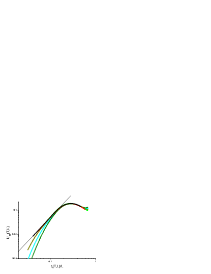
Figure 1: (Color on line) Bimodal $2$D ISG. Non-self-averaging parameter $U_{22}(T,L)$ against the normalized correlation length $\xi(T,L)/L$. $L=12$, $16$, $24$, $32$, $48$, $64$, $96$, $128$ from right to left. The straight line has slope $2$.

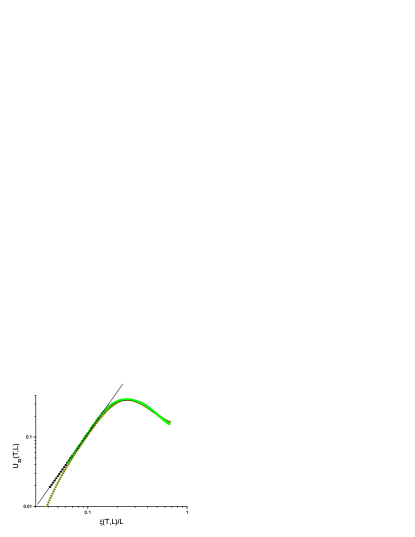
Figure 2: (Color on line) Bimodal $2$D ISG. Non-self-averaging parameter $U_{33}(T,L)$ against the normalized correlation length $\xi(T,L)/L$. $L=24$, $32$, $48$, $64$, $96$, $128$ from right to left. The straight line has slope $2$.

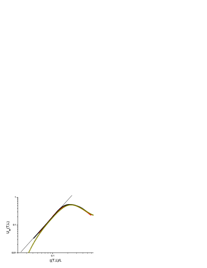
Figure 3: (Color on line)Bimodal $2$D ISG. Non-self-averaging parameter $U_{44}(T,L)$ against the normalized correlation length $\xi(T,L)/L$. $L=24$, $48$, $64$, $128$ from right to left. The straight line has slope $2$.

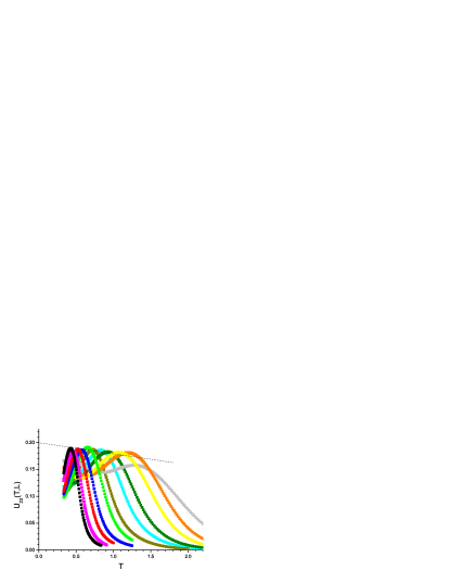
Figure 4: (Color on line) Bimodal $2$D ISG. Non-self-averaging parameter $U_{22}(T,L)$ against the temperature $T$. $L=128$, $96$, $64$, $48$, $32$, $24$, $16$, $12$, $8$, $6$, $4$ from left to right. The straight line extrapolates to criticality at $T=0$.

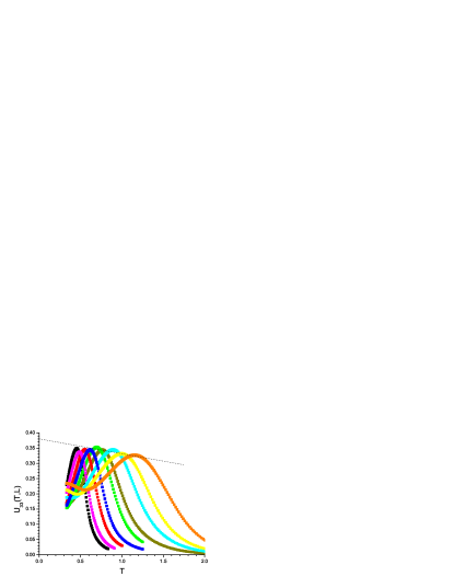
Figure 5: (Color on line) Bimodal $2$D ISG. Non-self-averaging parameter $U_{33}(T,L)$ against the temperature $T$. $L=128$, $96$, $64$, $48$, $32$, $24$, $16$, $12$, $8$, $6$ from left to right. The straight line extrapolates to criticality at $T=0$.

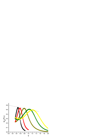
Figure 6: (Color on line) Bimodal $2$D ISG. Non-self-averaging parameter $U_{44}(T,L)$ against the temperature $T$. $L=8$, $16$, $32$, $64$, $128$ from right to left. The straight line extrapolates to criticality at $T=0$.

IV Dimension 3

The bimodal ISG in dimension 3 has a transition temperature for which the most recent estimate is $T_{c}=1.102(3)$ katzgraber:06 ; hasenbusch:08 ; baity:13 , and the Gaussian ISG has a transition temperature estimated to be $T_{c}=0.951(9)$ katzgraber:06 . The critical values of the dimensionless correlation length ratio $[\xi(T,L)/L]_{c}$ are estimated to be $0.652(3)$ and $0.635(10)$ respectively.

Hasenbusch, Pellisetto and Vicari hasenbusch:08 have generously posted their raw tabulated simulation data for the bimodal ISG in dimension 3 on the EPAPS site corresponding to their publication. In addition to the present measurements on $2^{13}$ samples of sizes $L=4,6,8,10,12$ we have extracted a selection of values of $U_{22}(\beta,L)$ from the tables of hasenbusch:08 , choosing the data sets with the largest numbers of temperatures, $L=16$, $20$, $24$. In each case the data correspond to measurements on about $10^{5}$ samples.

The $U_{22}(T,L)$ bimodal data in $3$D have almost $L$-independent peak values $U_{22}(T,L)_{\max}=0.207(3)$ with peak locations tending gradually downwards towards $T_{c}$ as $L$ increases, Fig. 8 (see palassini:03 who observed also a very similar peak height for a next-nearest-neighbor model). Small fluctuations as a function of $L$ can be put down to residual equilibration differences as the statistical errors in these data are very small because of the large numbers of samples. At the critical temperature the finite size scaling limit is $U_{22}(T_{c},L)=0.147$ hasenbusch:08 .

When scaled against $\xi(T,L)/L$, in the paramagnetic range $U_{22}(T,L)=[K_{3}\xi(T,L)/L]^{3}$ following the Aharony-Harris law, with $K_{3}=2.6(1)$, Fig. 7. The peak locations correspond to $\xi(T,L)/L\approx 0.35$.

In the large $L$ limit, the $U_{33}$ and $U_{44}$ peak locations are tending to $T_{c}$, and the peak values extrapolate to $U_{33}\sim 0.39$ and $U_{44}\sim 0.61$, Fig. 9 and 10.

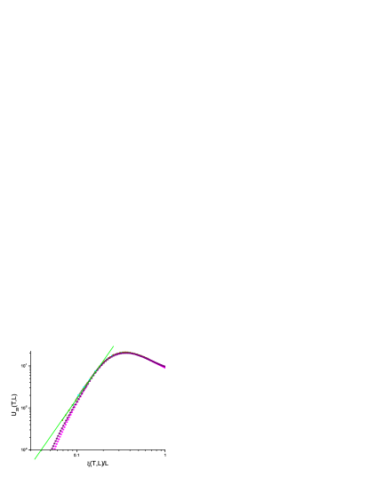
Figure 7: (Color on line) Bimodal 3D ISG. Non-self-averaging parameter $U_{22}(T,L)$ against the normalized correlation length $\xi(T,L)/L$. $L=10$, $12$, $16$, $20$, $24$ (pink, purple, cyan, green, black) right to left. $L=16$, $20$, $24$ from hasenbusch:08 . The straight line has slope 3.

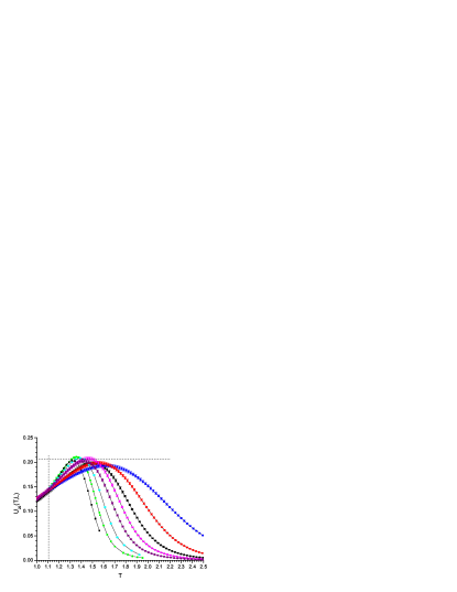
Figure 8: (Color on line) Bimodal 3D ISG. Non-self averaging parameter $U_{22}(T,L)$ against temperature $T$. $L=4$, $6$, $8$, $10$, $12$, $16$, $20$, $24$ (blue, red, black, pink, purple, cyan, green, brown) right to left. $L=16$, $20$, $24$ from hasenbusch:08 . Vertical line $T_{c}$.

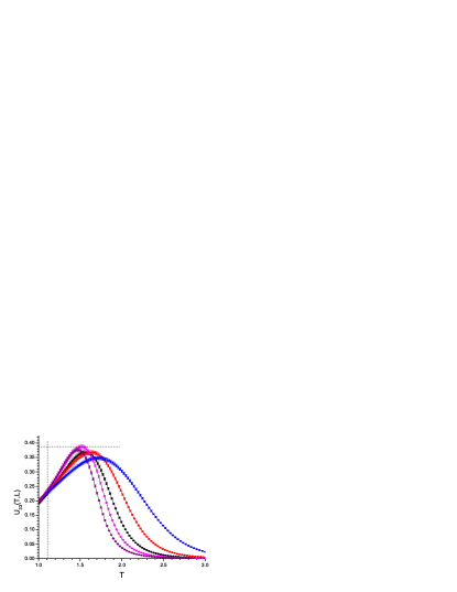
Figure 9: (Color on line) Bimodal 3D ISG. Non-self-averaging parameter $U_{33}(T,L)$ against temperature $T$. $L=4$, $6$, $8$, $10$, $12$ (blue, red, black, pink, purple) right to left. Vertical line $T_{c}$.

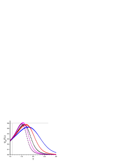
Figure 10: (Color on line) Bimodal 3D ISG. Non-self-averaging parameter $U_{44}(T,L)$ against temperature $T$. $L=4$, $6$, $8$, $10$, $12$ (blue, red, black, pink, purple) right to left. Vertical line $T_{c}$.

V Dimension 4

$U_{22}(T,L),U_{33}(T,L)$ and $U_{44}(T,L)$ data for the Gaussian ISG in dimension four are shown in Figs. 11, 12, 13, 14. The data correspond to $N=8192$ samples for each $L$. The critical temperature is $T_{c}=1.80(3)$ katzgraber:06 ; lundow:15 and the finite size critical value for the normalized correlation length ratio $[\xi/L]_{c}=0.440(5)$ katzgraber:06 ; lundow:15 . Scaling against the normalized correlation length Fig. 11, $U_{22}(T,L)=(K_{4}\xi(T,L)/L)^{4}$ again following the Aharony-Harris law, with $K_{4}=2.7(1)$ and peaks located at $\xi(T,L)/L=0.43(2)$ so very close to $\xi(T_{c},L)/L$.

Data obtained for the $4$D bimodal ISG (not shown) follow a very similar pattern with the same peak height. The locations of the $U_{nn}(T,L)$ peaks are almost independent of $L$. This was noted for $U_{22}(T,L)$ in the $4$D Gaussian ISG in Ref. palassini:03 , and in Ref. jorg:08 for a bond-diluted bimodal model; it follows from the proximity of the peak $\xi(T,L)/L$ and critical $\xi(T_{c},L)/L$ values. For the bond-diluted bimodal model, the peak height is $\approx 0.205$ jorg:08 . Because of the quasi-$L$-independence, the peak location extrapolated to infinite size provides an estimate for $T_{c}$ which is limited in precision only by the statistical uncertainties.

The Gaussian $U_{nn}(T,L)$ peak heights become independent of $L$ to within the statistical errors after weak finite size effects for small $L$, Figs. 12, 13, 14. The peak height values $U_{22}(T,L)_{\max}=0.210(5)$, $U_{33}(T,L)_{\max}=0.400(5)$, $U_{44}(T,L)_{\max}=0.63(2)$ are the same as those in dimensions $2$ and $3$ to within the statistical precision. The stability of the $U_{nn}(T,L)$ peak heights as $L$ is varied turns out to be a useful empirical criterion for the quality of equilibration.

Alternatively, considering the $U_{nn}(T,L)$ as dimensionless variables, the intersections of the curves for fixed $L$ should also give a criterion for estimating $T_{c}$, but the statistical fluctuations and corrections to scaling affect the intersections much more drastically than they do the peak location, which means that this is an imprecise criterion in the $4$D case as noted by jorg:08 .

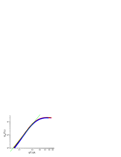
Figure 11: (Color on line) Gaussian 4D ISG. Non-self-averaging parameter $U_{22}(T,L)$ against the normalized correlation length $\xi/LT,L)/L$. $L=4$, $6$, $8$, $10$, $12$ (blue, red, black, pink, green). The straight line has slope 4.

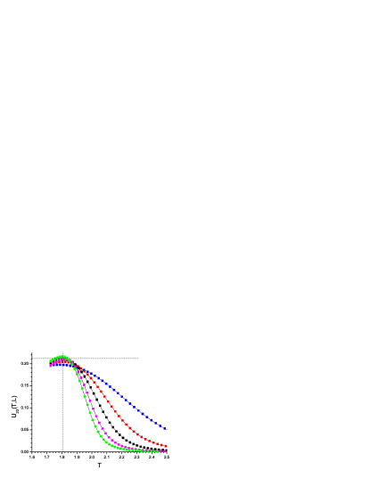
Figure 12: (Color on line) Gaussian 4D ISG. Non-self-averaging parameter $U_{22}(T,L)$ against the temperature $T$. $L=4$, $6$, $8$, $10$, $12$ (blue, red, black, pink, green) from right to left. The horizontal line is an extrapolation to criticality at $T=T_{c}$ (vertical line).

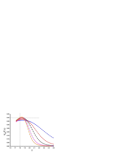
Figure 13: (Color on line) Gaussian 4D ISG. Non-self-averaging parameter $U_{33}(T,L)$ against the temperature $T$.$L=4$, $6$, $8$, $10$, $12$ (blue, red, black, pink, green) from right to left. The horizontal line is an extrapolation to criticality at $T=T_{c}$ (vertical line).

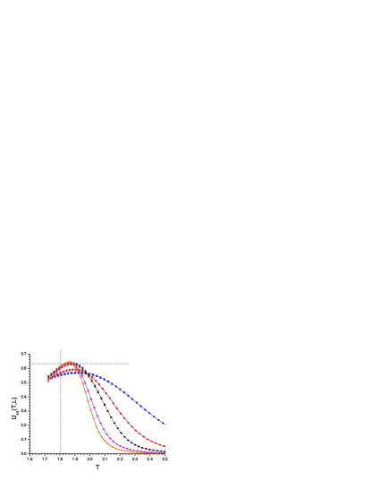
Figure 14: (Color on line) Gaussian 4D ISG. Non-self-averaging parameter $U_{44}(T,L)$ against the temperature $T$ . $L=4$, $6$, $8$, $10$, $12$ (blue, red, black, pink, green) from right to left. The horizontal line is an extrapolation to criticality at $T=T_{c}$ (vertical line).

VI Dimension 5

$U_{22}(T,L),U_{33}(T,L)$ and $U_{44}(T,L)$ data for the Gaussian ISG in dimension five are shown in Figs. 15, 16, 17, 18. The data correspond to $4096$ samples for each $L$. The critical temperature is $T_{c}=2.390(5)$ and the finite size critical value for the normalized correlation length ratio $[\xi/L]_{c}\approx 0.45$ lundow:15b . We are not aware of other comparable simulation measurements in this dimension. Data obtained for the $5$D bimodal ISG (not shown) are very similar. The $U_{nn}(T,L)$ peak heights become independent of $L$ to within the statistical errors after weak finite size effects for small $L$. The peak height values $U_{22}(T,L)_{\max}=0.215(5)$, $U_{33}(T,L)_{\max}=0.405(5)$, $U_{44}(T,L)_{\max}=0.64(2)$ are again practically the same as those in dimensions $2,3$ and $4$ to within the statistical precision.

When scaled against the correlation length ratio, in the paramagnetic range $U_{22}(T,L)=[K_{5}\xi(T,L)/L]^{5}$ following the Aharony-Harris law aharony:96 , with $K_{5}=2.5(1)$. The peak locations correspond to $\xi(T,L)/L\approx 0.50$. As this ratio is greater than $[\xi/L]_{c}$ the locations of the $U{nn}(T,L)$ peaks are at temperatures below $T_{c}$ and the peak temperatures move upwards towards $T_{c}$ with increasing $L$. The peak location extrapolated to infinite size provides an estimate for $T_{c}$ which is again limited by the statistical precision but which provides a useful independent check on the value of the ordering temperature.

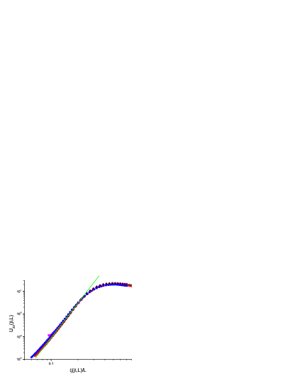
Figure 15: (Color on line) Gaussian 5D ISG. Non-self-averaging parameter $U_{22}(T,L)$ against the normalized correlation length $\xi(T,L)/L$. $L=4$, $6$, $8$, $10$ (blue, red, black, pink). The straight line has slope 5.

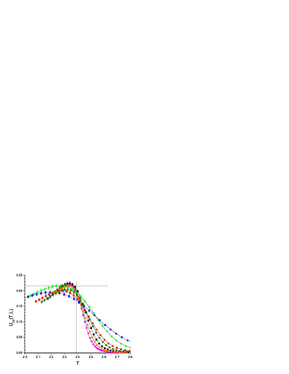
Figure 16: (Color on line) Gaussian 5D ISG. Non-self-averaging parameter $U_{22}(T,L)$ against the temperature$T$. $L=4$, $5$, $6$, $7$, $8$, $9$, $10$ (blue, green, red, olive, black, orange, pink) from right to left on the right. The horizontal line is an extrapolation to criticality at $T=T_{c}$. (vertical line)

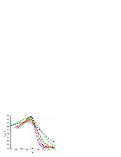
Figure 17: (Color on line) Gaussian 5D ISG. Non-self-averaging parameter $U_{33}(T,L)$ against the temperature $T$.$L=4$, $5$, $6$, $7$, $8$, $9$, $10$ (blue, green, red, olive, black, orange, pink) from right to left on the right. The horizontal line is an extrapolation to criticality at $T=T_{c}$. (vertical line)

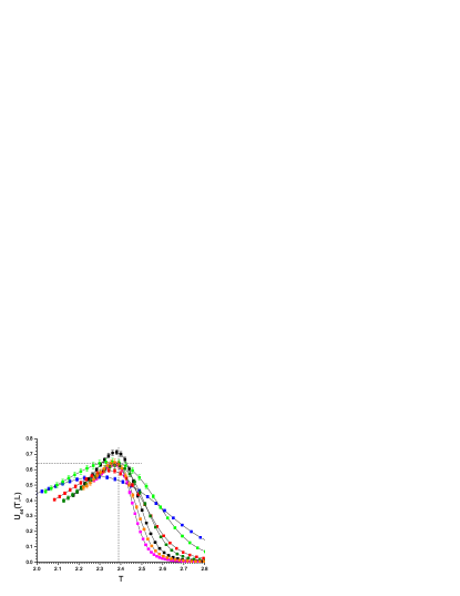
Figure 18: (Color on line) Gaussian 5D ISG. Non-self-averaging parameter $U_{44}(T,L)$ against the temperature $T$. $L=4$, $5$, $6$, $7$, $8$, $9$, $10$ (blue, green, red, olive, black, orange, pink) from right to left on the right. The horizontal line is an extrapolation to criticality at $T=T_{c}$. (vertical line)

VII Dimension 7

By this dimension, $N$ the number of spins per sample has become very large, ($N=823,543$ for $L=7$), which imposes practical limits on the sizes and numbers of samples in the simulations. The simulations were carried out for $L=3$ to $7$ with $512$ samples at each $L$.

The dimension $7$ bimodal ISG has an ordering temperature $T_{c}=3.39(1)$ estimated using the standard Binder cumulant crossing point technique lundow:15b in agreement with the high temperature series expansion (HTSE) estimates $T_{c}=3.37(2)$ singh:86 and $T_{c}=3.384(15)$daboul:04 . (Curiously the HTSE value given in Ref. klein:91 corresponds to $T_{c}=3.459$. We suspect a typographical error). As this dimension is above the upper critical dimension $d=6$, the critical exponents $\gamma=1$ and $\nu=1/2$ are known exactly. In this case in the paramagnetic regime $U_{22}(T,L)=(K_{7}\xi(T,L)/L)^{6}$, with an exponent which appears to be $\approx 6$ rather than $7$, Fig. 19. This could arise from the breakdown of the relations between scaling exponents above the ucd. Because of the limited number of samples and the small values of $L$ at this dimension, this estimate is not very precise.

In the plot of $U_{22}(T,L)$ against $T$, Fig. 20, the $L$-independent critical finite size crossing point value is $U_{22}(T_{c})\approx 0.15$, and the $[U_{22}(T,L)]_{\max}$ peak heights are independent of $L$ and equal to $\approx 0.21$ to within the statistics, as for the other dimensions. The maxima locations move towards $T_{c}$ from within the ordered regime. This behavior is very similar to that observed in the mean field ISG SK model hukushima:00 ; picco:01 .

The higher order $U_{33}(T,L)$ and $U_{44}(T,L)$, Fig. 21 and Fig. 22, follow much the same pattern, with peak maxima of $0.39(1)$ and $0.61(2)$ respectively, again equal to the values for the other dimensions to within the statistics.

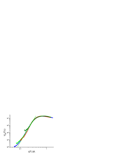
Figure 19: (Color on line) Bimodal 7D ISG. Non-self-averaging parameter $U_{22}(T,L)$ against the normalized correlation length $\xi(T,L)/L$. $L=4$, $5$, $6$, $7$ (blue, green, red, olive). The straight line has slope 6.

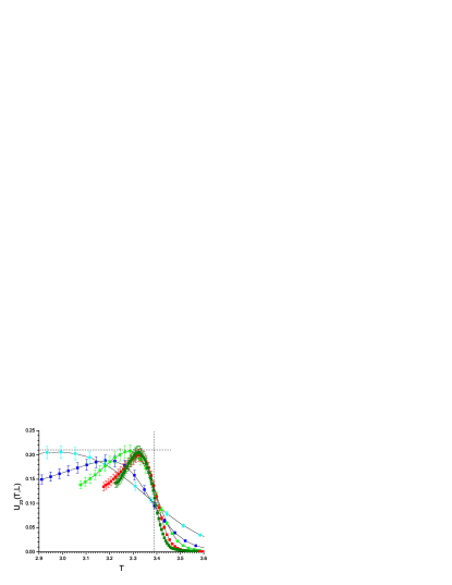
Figure 20: (Color on line) Bimodal 7D ISG. Non-self averaging parameter $U_{22}(T,L)$ against temperature $T$. $L=3$, $4$, $5$, $6$, $7$ (cyan, blue, green, red, olive) right to left. Vertical line $T_{c}$.

Figure 21: (Color on line) Bimodal 7D ISG. Non-self averaging parameter $U_{33}(T,L)$ against temperature $T$. $L=3$, $4$, $5$, $6$, $7$ (cyan, blue, green, red, olive) right to left. Vertical line $T_{c}$.

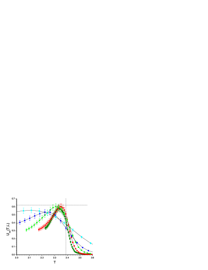
Figure 22: (Color on line) Bimodal 7D ISG. Non-self averaging parameter $U_{44}(T,L)$ against temperature $T$. $L=3$, $4$, $5$, $6$, $7$ (cyan, blue, green, red, olive) right to left. Vertical line $T_{c}$.

VIII The Gauge Glass

The Gauge glass (GG) is a vector spin glass which does not support chiral ordering. The GG in dimension $3$ has a critical temperature $T_{c}=0.47(1)$ olson:00 ; katzgraber:04 ; alba:11 . The non-self-averaging parameter $U_{22}(L,T)$ scales with $\xi(L,T)/L$ alba:11 and shows a maximum peak height independent of $L$ and a peak position $T_{\max}(L)$ near $\xi(L,T)/L=0.35$. The paramagnetic regime data alba:11 appear by inspection to be compatible with the Aharony-Harris rule $U_{22}(L,T)\sim[\xi(L,T)/L]^{3}$ although the published data are not presented in this way. As the critical correlation length ratio is $[\xi(L,T)/L]_{c}=0.54$ alba:11 , the $U_{22}(L,T)$ peak temperature location moves downwards with $L$ and tends towards $T_{c}$. The $3$D vector spin glass GG $U_{22}(T,L)$ thus follows basically the same rules as followed by $U_{22}(T,L)$ in the Ising spin glass in $3$D, except that the GG peak maximum is $\approx 0.10$ instead of $0.205$. Data on GGs in dimensions $2,3$ and $4$ from measurements which were not designed to estimate the non-self-averaging parameter katzgraber:04 are consistent with $U_{22}(T,L)$ peak values near $0.10$ in each dimension. We can speculate that this family of spin glass models also has its characteristic dimension-independent value of the non-self-averaging peak height.

IX Heisenberg and XY spin glasses

Numerical measurements on Heisenberg spin glasses (HSGs) are of particular importance because the canonical experimental spin glass dilute alloys (AuFe, CuMn, AgMn) are all Heisenberg systems, so it should be possible to understand the ordering mechanism in ”real life” spin glasses on the basis of numerical data on Heisenberg models. We have no new data to report on these models but it is of interest to consider published non-self-averaging data in the light of the ISG results.

Both Heisenberg and XY spin glasses can support chiral glass order as well as spin glass order, and for many years there have been two conflicting interpretations of the numerical data on the ordering transitions in these models in dimension $3$. According to the first interpretation, the ordering is spin-spin interaction driven; basically the ordering process is much the same as in ISGs, and the chiral order follows on as a geometrically necessary consequence of the onset of spin order, without the chiral interactions playing any significant role in the spin glass transition lee:03 ; campos:06 ; lee:07 ; pixley:08 ; fernandez:09 . The alternative interpretation is that the driving role in $3$D HSG or XYSG ordering is played by the chirality, so that there is first a chiral order onset followed at a lower temperature by spin ordering transition kawamura:10 ; hukushima:05 ; viet:09 ; obuchi:13 . (Similar disagreements concerning fully frustrated $2$D XY models were resolved definitively in favor of a distinct chiral order transition just above a spin order transition hasenbusch:05 ; okumura:11 ). The arguments of both schools to support their respective interpretations in the $3$D HSG and XYSG models have been essentially based on analyses of the data for the crossing points of the dimensionless normalized spin and chiral ($s$ and $c$) correlation lengths $\xi_{s}(T,L)/L$ and $\xi_{c}(T,L)/L$. The numerical simulations in the spin glasses are even more demanding than in the fully frustrated models, and because of intrinsic finite size corrections and the need to reach strict equilibration at each $L$, extrapolations to infinite $L$ in order to estimate the ThL crossing point locations are delicate. As simulations were extended to larger sizes in successive Gaussian HSG and XYSG measurements interpreted on the spin-driven ordering scenario, the joint spin/chiral crossover temperature was estimated to be $T_{c}(HSG)\approx 0.160$ lee:03 , $T_{c}(HSG)\approx 0.145$ with a KTB-like critical line campos:06 , marginal but very similar spin and chiral behavior (XYSG and HSG)lee:07 ; pixley:08 , and most recently $T_{c}(HSG)\approx 0.120$ fernandez:09 . No non-self-averaging results were reported. From detailed $3$D bimodal and Gaussian HSG and $3$D Gaussian XYSG measurements, the two separate transition temperatures on the chiral-driven ordering scenario are estimated to be (bimodal HSG) hukushima:05 , $T_{c}(c)=0.194(5)$ and $T_{c}(s)\leq 0.15$, (Gaussian HSG) $T_{c}(c)=0.143(3)$ and $T_{c}(s)=0.125(+0.006/-0.012)$ viet:09 , and (XYSG) $T_{c}(c)=0.308(5)$ and $T_{c}(s)=0.274(3)$ obuchi:13 . Non-self-averaging data were shown in each case.

In the light of the ISG results reported above, it would appear that in Heisenberg and XY spin glasses non-self-averaging could provide an independent primary numerical criterion for spin and/or chiral ordering much less sensitive to finite size effects and to strict equilibration (as already suggested in Ref. hukushima:05 ). On the first (spin-driven ordering) scenario one would expect the spin non-self-averaging parameter $U_{22s}(T,L)$ to follow much the same rules as for the ISG or the GG chiral-free vector spin glass cases discussed above, with a peak location moving towards an upper spin ordering temperature $T_{c}(s)$ as $L$ increases, and a regular behavior reflecting $U_{22s}(T,L)\sim(\xi_{s}(T,L)/L)^{3}$ in the paramagnetic regime above $T_{c}(s)$. On this interpretation the chiral $U_{22c}(T,L)$ would be weaker than the $U_{22s}(T,L)$; if a $U_{22c}(T,L)$ peak exists, it would be located at a temperature below or possibly at the ThL $U_{22s}(T,L)$ peak.

On the second (chiral-driven order) scenario, it would be the chiral $U_{22c}(T,L)$ which would show a peak first, with a peak location tending towards the (upper) chiral ordering temperature $T_{c}(c)$ as $L$ increases. In the paramagnetic regime one would expect a regular behavior of the chiral non-self-ordering $U_{22c}(T,L)$ with increasing $L$, governed by $U_{22c}(T,L)\sim(\xi_{c}(T,L)/L)^{3}$. On this scenario the spin $U_{22s}(T,L)$ would then show a peak location somewhere below the chiral $U_{22c}(T,L)$ peak, with a location tending towards an ordering temperature $T_{c}(s)$ below $T_{c}(c)$, together with a paramagnetic regime $U_{22s}(T,L)$ behavior behaving irregularly at least at small $L$ because the paramagnetic spin ordering is perturbed by the dominant onset of chiral order.

Very informative non-self-averaging data have been published on the $3$D HSG with bimodal interactions hukushima:05 , on the $3$D HSG with Gaussian interactions viet:09 , and on the $3$D Gaussian XYSG obuchi:13 . In each case the pattern is the same :

- there is a strong $U_{22c}(T,L)$ peak at an almost $L$-independent temperature $T\approx 0.19$, $T\approx 0.145$, $T\approx 0.31$ respectively, so in each case close to the $T_{c}(c)$ value estimated independently from other criteria hukushima:05 ; viet:09 ; obuchi:13 . In the paramagnetic regime there is a regular narrowing in temperature of the $U_{22c}(T,L)$ peak with increasing $L$ which appears compatible with the Aharony-Harris law $U_{22c}(T,L)\sim(\xi_{c}(T,L)/L)^{3}$ though the data are not presented in this form.

- in each case, the spin $U_{22s}(T,L)$ peak is either not visible (HSGs) or is marginal (XYSG) down to the lowest temperature at which non-self-averaging measurements were made, $T\approx 0.145$,$T\approx 0.11$ to $0.13$ depending on $L$, and $T\approx 0.24$ to $0.275$ depending on $L$ in the three cases. Over the whole temperature range $U_{22s}(T,L)$ is always weaker than $U_{22c}(T,L)$, and $U_{22s}(T,L)$ has irregular behavior as a function of $L$ in the paramagnetic temperature regime at and above the $U_{22c}(T,L)$ peak.

Thus the non-self-averaging data $U_{22c}(T,L)$ and $U_{22s}(T,L)$ in the three models hukushima:05 ; viet:09 ; obuchi:13 can be seen by inspection to be clearly incompatible with the behavior expected on the spin-driven ordering scenarios lee:03 ; campos:06 ; lee:07 ; pixley:08 ; fernandez:09 , and fully compatible with the chiral-driven ordering interpretationkawamura:10 ; hukushima:05 ; viet:09 ; obuchi:13 .

X Conclusion

The non-self-averaging data on ISGs in all dimensions show a remarkable regularity. In each dimension there is a peak as a function of temperature in the standard non-self-averaging parameter $U_{22}(T,L)$ and in the higher order parameters $U_{33}(T,L)$ and $U_{44}(T,L)$ whose values are $L$-independent after weak small size effects; the peak values $U_{22}(T,L)_{\max}\approx 0.21$, $U_{33}(T,L)_{\max}\approx 0.40$, $U_{44}(T,L)_{\max}\approx 0.62$ are independent of dimension to within the statistics for dimensions $2,3,4,5$ and $7$. In the paramagnetic regime above the peak the Aharony-Harris renormalization group law aharony:96 $U_{nn}(T,L)=(K_{d}\xi(T,L)/L)^{d}$ is obeyed, with $K_{d}(U_{22})\approx 2.6$ for all dimensions. Both of these empirical observations can be classed as “hyperuniversal behavior”.

Published alba:11 and unpublished katzgraber:04 data on the Gauge Glass, a vector spin glass which does not support chirality, suggest that non-self-averaging rules analogous to those that hold in the ISGs appear to apply but with a different characteristic peak height $U_{22}(T,L)_{\max}\approx 0.10$.

XY and Heisenberg spin glasses can support chiral ordering as well as spin ordering. In the light of the non-self-averaging behavior reported above for the ISG models, it is clear that the published spin and chiral non-self-averaging data hukushima:05 ; viet:09 ; obuchi:13 in $3$D Heisenberg and $XY$ models are incompatible with a spin-driven ordering scenario lee:03 ; campos:06 ; lee:07 ; pixley:08 ; fernandez:09 but strongly support the alternative conclusion that the spin glass ordering in these models is chiral-driven rather than spin-driven, on the Kawamura scenario kawamura:10 . An important implication is that order in the canonical experimental Heisenberg spin glasses is also chirality driven.

- (1) A. Aharony and A. B. Harris, Phys. Rev. Lett. 77, 3700 (1996).
- (2) A. K. Hartmann and A. P. Young, Phys. Rev. B 64,18404 (2001).
- (3) M. Ohzeki and H. Nishimori, J. Phys. A: Math. Theor. 42, 332001 (2009).
- (4) P. H. Lundow and I. A. Campbell, Phys. Rev. E 91, 042121 (2015), Physica A 434, 181 (2015).
- (5) P. H. Lundow and I. A. Campbell, arXiv:1506.07141.
- (6) T. Jörg, J. Lukic, E. Marinari, O. C. Martin, Phys. Rev. Lett. 96 237205 (2006).
- (7) F. Parisen Toldin, A. Pelissetto, and E. Vicari, Phys. Rev. E 82, 021106 (2010), Phys. Rev. E 84, 051116 (2011).
- (8) H. G. Katzgraber, M. Körner, and A. P. Young, Phys. Rev. B 73, 224432 (2006)
- (9) M. Hasenbusch, A. Pelissetto, and E. Vicari, Phys. Rev. B 78, 214205 (2008), and EPAPS Document No. E-PRBMDO-78-003845.
- (10) M. Baity-Jesy et al, Phys. Rev. B 88, 224416 (2013).
- (11) M. Palassini, M. Sales, and F. Ritort, Phys. Rev. B 68, 224430 (2003).
- (12) R. A. Baños, L. A. Fernandez, V. Martín-Mayor, and A. P. Young, Phys. Rev. B 86, 134416 (2012).
- (13) T. Jörg and H. G. Katzgraber, Phys. Rev. Lett. 101, 197205 (2008).
- (14) P. H. Lundow and I. A. Campbell, unpublished.
- (15) R. R. P. Singh and S. Chakravarty, Phys. Rev. Lett. 57, 245 (1986).
- (16) D. Daboul, I. Chang, and A. Aharony, Eur. Phys. J. B 41, 231 (2004).
- (17) L. Klein, J. Adler, A. Aharony, A. B. Harris, and Y. Meir, Phys. Rev. B 43, 11249 (1991).
- (18) K. Hukushima and H. Kawamura Phys. Rev. E 62, 3360 (2000).
- (19) M. Picco, F. Ritort and M. Sales, Eur. Phys. J. B 19, 565 (2001).
- (20) T. Olson and A. P. Young, Phys. Rev. B 61, 12467 (2000).
- (21) V. Alba and E. Vicari, Phys. Rev. B 83, 094203 (2011).
- (22) H. G. Katzgraber and I. A. Campbell, Phys. Rev. B 69, 094413 (2004).
- (23) L. W. Lee and A. P. Young, Phys. Rev. Lett. 90, 227203 (2003).
- (24) I. Campos, M. Cotallo-Aban, V. Martín-Mayor, S. Perez-Gaviro, and A. Tarancon, Phys. Rev. Lett. 97, 217204 (2006).
- (25) L. W. Lee and A. P. Young, Phys. Rev. B 76, 024405 (2007).
- (26) J. H. Pixley and A. P. Young, Phys. Rev. B 78, 014419 (2008).
- (27) L. A. Fernandez , V. Martín-Mayor, S. Perez-Gaviro, A. Tarancon and A. P. Young, Phys. Rev. B 80, 024422 (2009).
- (28) H. Kawamura, J. Phys. Soc. Jpn. 79, 011007 (2010).
- (29) K. Hukushima and H. Kawamura, Phys. Rev. B 72, 144416 (2005).
- (30) D. X. Viet and H. Kawamura, Phys. Rev. Lett. 102, 027202 (2009); Phys. Rev. B 80, 064418 (2009).
- (31) T. Obuchi and H. Kawamura, Phys. Rev. B 87, 174438 (2013).
- (32) M. Hasenbusch, A. Pelissetto, and E. Vicari, Phys. Rev. B 72, 184502 (2005).
- (33) S. Okumura, H. Yoshino, and H. Kawamura, Phys. Rev. B 83, 094429 (2011).