Abstract

Membranes in M-theory are expected to interact via splitting and joining processes. We study these effects in the pp-wave matrix model, in which they are associated with transitions between states in sectors built on vacua with different numbers of membranes. Transition amplitudes between such states receive contributions from BPS instanton configurations interpolating between the different vacua. Various properties of the moduli space of BPS instantons are known, but there are very few known examples of explicit solutions. We present a new approach to the construction of instanton solutions interpolating between states containing arbitrary numbers of membranes, based on a continuum approximation valid for matrices of large size. The proposed scheme uses functions on a two-dimensional space to approximate matrices and it relies on the same ideas behind the matrix regularisation of membrane degrees of freedom in M-theory. We show that the BPS instanton equations have a continuum counterpart which can be mapped to the three-dimensional Laplace equation through a sequence of changes of variables. A description of configurations corresponding to membrane splitting/joining processes can be given in terms of solutions to the Laplace equation in a three-dimensional analog of a Riemann surface, consisting of multiple copies of $\mathbbm{R}^{3}$ connected via a generalisation of branch cuts. We discuss various general features of our proposal and we also present explicit analytic solutions.

1 Introduction

The best candidate for a microscopic description of M-theory is the matrix model originally proposed in [1] as a regularisation of the supermembrane theory and subsequently conjectured in [2] to describe the full dynamics of the theory in light-front quantisation when the size of the matrices is sent to infinity. The matrix model provides a formulation of M-theory which is capable of describing multi-membrane configurations, arising as block-diagonal matrices. Membranes in M-theory should interact via splitting and joining processes and therefore the matrix model should capture such effects. However, no concrete proposal for the description of these splitting/joining interactions in the matrix model has been formulated. More generally there is no quantitative prescription for the study of this type of membrane interactions, which would make it possible to evaluate the associated transition amplitudes. This makes it difficult to test any results for these amplitudes that may be obtained from the matrix model. This is of course a general difficulty with all predictions of the matrix model, which so far have been mostly tested at the level of the low energy supergravity approximation.

The AdS/CFT correspondence – and specifically the duality proposed in [3], relating M-theory in AdS${}_{4}\times S^{7}/\mathbbm{Z}_{k}$ to an ${\mathcal{N}}=6$ Chern–Simons theory – provides in principle new means of testing the matrix model predictions by comparing them to a dual CFT. In the context of the duality of [3] it was recently shown in [4] that the matrix model description of M-theory in AdS${}_{4}\times S^{7}/\mathbbm{Z}_{k}$ can be quantitatively compared to the dual gauge theory without relying on the supergravity approximation or compactification to type IIA string theory in ten dimensions. The crucial observation of [4] was that, focussing on large angular momentum states in M-theory and the dual CFT sector involving monopole operators, natural approximation schemes arise on the two sides of the duality, so that a systematic, quantitative comparison is possible.

On the gravity side, M-theory states with large angular momentum, $J$, along a great circle in $S^{7}$ can be studied using the pp-wave approximation. The associated matrix model uses $J\times J$ matrices and its action was constructed in [5]. We will use basic properties of the model which were further studied in [6]. Multi-membrane states in the pp-wave matrix model consist of concentric membranes and their fluctuations. More precisely the vacua of the theory consist of spherical membranes which extend in AdS₄ directions and are point-like in $S^{7}$. They are classified by a set of integers, $J_{i}$, $i=1,\ldots,n$, corresponding to a partition of the total angular momentum among $n$ membranes. The fluctuations of the spherical membranes described by the pp-wave matrix model are associated, in the dual gauge theory, with certain monopole operators. The latter are characterised by their integer GNO charges, which are in one-to-one correspondence with the angular momenta, $J_{i}$, of the membranes. The sector of monopole operators with large GNO charges can be reliably studied using a weakly-coupled effective low-energy approximation.

The AdS₄/CFT₃ duality in this M-theoretic regime relates correlation functions of monopole operators in the ABJM theory to processes on the gravity side in which the dual states interact in the bulk and propagate to the boundary. The simplest such process involves a single membrane splitting into two – with the associated three states propagating to the boundary – and it corresponds to a three-point correlation function of monopole operators. Similar processes have been studied in the case of the AdS₅/CFT₄ correspondence, in which three-point functions of gauge-invariant operators are related to cubic interaction vertices in the bulk associated with the splitting of strings in the pp-wave approximation. A method to compare the cubic vertices in string theory to the corresponding conformal three-point functions in the CFT was discussed in [7], following a spacetime interpretation first proposed in [8]. Studies using other approaches can be found in  [9, 10, 11, 12, 13, 14]. Similar aspects have been extensively studied beyond the pp-wave approximation taking advantage of the integrability appearing in the analysis of the system. For recent interesting developments and up-to-date references, see [15, 16].

The three-point correlation functions of monopole operators, in particular those with large charge $J$, which are relevant in the present case, are well defined in the ABJM theory and one expects that they should be computable within the CFT framework. Although in this paper we focus on the gravity side of the correspondence, it is important that in principle the results of the matrix model calculation can be verified by independent means. Successfully comparing the physical transition amplitudes associated with a membrane splitting or joining process to the gauge theory results for three-point functions would provide such an independent test. The agreement would not only represent a highly non-trivial test of the AdS₄/CFT₃ correspondence, but it would also provide strong evidence indicating that the matrix model captures the aspects of the dynamics of membranes related to splitting/joining interactions.

In the context of the pp-wave matrix model, processes of joining or splitting of membranes correspond to transitions between states built on vacua with different numbers of membranes. A semi-classical description of these transitions can be given in terms of tunnelling amplitudes associated with instanton configurations which interpolate between states containing different numbers of membranes. In this paper we initiate a study of these interpolating configurations. The relevant instantons are BPS solutions to the Euclidean equations of motion of the pp-wave matrix model [17], with boundary conditions specifying the single or multiple membrane states between which they interpolate. The equations obeyed by these BPS instantons, with the same boundary conditions, were studied in a different context in [18], where they were found to arise as the equations describing domain walls interpolating between distinct isolated vacua of the so-called ${\mathcal{N}}=1^{*}$ SYM theory. A number of properties of these instanton equations and the associated moduli spaces were studied in [18]. An important ingredient in the analysis presented in [18] is the observation that the relevant instanton equations can be mapped to the Nahm equations [19] which arise in the construction of BPS monopoles, although with different boundary conditions.

The BPS instantons of the pp-wave matrix model are saddle points representing the dominant contribution to the tunnelling processes. Physical transition amplitudes associated with the splitting/joining processes can be computed using a semi-classical approximation around the instanton solutions. This involves evaluating the determinants arising from the non-zero mode fluctuations as well as the integration over the collective coordinates associated with zero modes. Although there may be alternative approaches to the computation of the splitting/joining transition amplitudes, in order to carry out the standard semi-classical calculations it is necessary to obtain the explicit form of the classical instanton solutions. However, although various general features of the instanton equations – including conditions for the existence of solutions and properties of their moduli spaces – were studied in [18], little is known about explicit solutions. In particular, no solution is known for the most elementary process we are interested in, i.e. the splitting of a single membrane into two.

In this paper we show that an efficient approach to the construction of solutions to the instanton equations as well as to the study of their moduli spaces can be developed using a continuum approximation. Such an approximation scheme is valid in the case of large matrices and, therefore, it is applicable in the context of the M-theoretic regime of the AdS₄/CFT₃ duality considered in [4]. In this approximation the original instanton equations can be mapped to a continuum version of the Nahm equations, which in turn can be shown to be equivalent to the three-dimensional Laplace equation, using results in [20, 21, 22]. In this formulation equipotential surfaces for the solution to the Laplace equation directly represent the profile of the membranes at different times. Using this approach we present explicit analytic solutions describing the splitting of membranes.

A remarkable feature of our construction is that, in order to obtain a solution representing the splitting of one membrane into two, we are led to consider the Laplace equation not in the ordinary three-dimensional Euclidean space, but rather in a three-dimensional generalisation of a two-sheeted Riemann surface, which we refer to as a Riemann space following [23]. The emergence of Riemann spaces, which can be naturally motivated in the context of the construction of our solutions, is quite intriguing. The possibility that in the description of membrane interactions Riemann spaces may play a central role, similar to that played by Riemann surfaces in string perturbation theory, is very interesting and deserves further investigation.

This paper is organised as follows. In section 2 we describe the instanton equations and we recall some general properties of their solutions and of the associated moduli space which were obtained in [18]. In section 3 we discuss the continuum approximation scheme used in our analysis and the mapping of the instanton equations to the three-dimensional Laplace equation. In section 4 we present explicit solutions to the Laplace equation which are relevant for the pp-wave matrix model and we describe the corresponding solutions to the BPS instanton equation within our continuum approximation. The most interesting solution – which utilises a two-sheeted Riemann space to describe the splitting of a single membrane into two – is considered in section 4.2. We conclude with a discussion of our results in section 5. Technical details are discussed in various appendices.

2 BPS instantons

In our study of configurations describing membrane splitting/joining processes we focus on the pp-wave matrix model [5]. As discussed in [4] this model provides a good approximation to the dynamics of M-theory in AdS${}_{4}\times S^{7}/\mathbbm{Z}_{k}$ in a sector containing membranes with large angular momentum, $J$. M-theory in this background is dual to the $\mathcal{N}=6$ Chern-Simons theory with gauge group U($N$)$\times$ U($N$) and level $k$ constructed in [3]. The region of applicability of the pp-wave approximation is defined by the conditions $1\ll J\ll(Nk)^{1/2}$. Moreover for $J\gg(Nk)^{1/3}$ the model is weakly coupled.

In this section we review the BPS instanton equations of the pp-wave matrix model and recall some of their properties. These equations were first studied in a different context in [18], where they were shown to describe supersymmetric domain walls interpolating between vacua of the ${\mathcal{N}}=1^{*}$ SYM theory. Their relevance in the pp-wave matrix model was pointed out in [17], where they were first shown to describe instanton configurations interpolating between different vacua.

2.1 Instanton equations

The Euclidean action describing the M-theory side of the AdS₄/CFT₃ duality in the large $J$ sector takes the form [5, 6, 4]

$$S_{E}=\int{\rm d}t\;\text{tr} \biggl{\{}\frac{k}{2R}\left(\frac{DY^{i}}{Dt}\right)^{2}+\frac{k}{2R}\left(\frac{DX^{m}}{Dt}\right)^{2}+(2\pi T)^{2}\frac{R}{4k}\left((i[X^{m},X^{n}])^{2}+2(i[X^{m},Y^{i}])^{2}\right)$$

$$+\frac{k}{2R^{3}}(X^{m})^{2}+(2\pi T)^{2}\frac{R}{2k}\left(\frac{i}{2}\epsilon_{ijk}[Y^{j},Y^{k}]+\frac{1}{2\pi T}\frac{2k}{R^{2}}Y^{i}\right)^{\!\!2}$$ (2.1)

$$+\frac{1}{2}\Psi^{T}\frac{D\Psi}{Dt}+2\pi T\frac{R}{k}\frac{1}{2}\left(\Psi^{T}\gamma^{m}[X^{m},\Psi]+\Psi^{T}\gamma^{i}[Y^{i},\Psi]\right)-\frac{3i}{4}\frac{1}{R}\,\Psi^{T}\gamma^{123}\Psi\biggl{\}},$$

where $T=1/[(2\pi)^{2}l_{P}^{3}]$ is the membrane tension, $R$ is the radius of $S^{7}$ (and twice the radius of AdS₄) and $\gamma^{\alpha}$ $(\alpha=1,2,\ldots,9)$ are SO($9$) gamma matrices, with $\gamma^{123}=\gamma^{1}\gamma^{2}\gamma^{3}$. Following the notation in [4], we have denoted by $Y^{i}$ $(i=1,2,3)$ and $X^{m}$ $(m=4,5,\ldots,9)$ matrices originating from the membrane coordinates in AdS₄ and $S^{7}$ respectively. $\Psi$ is a 16 component matrix valued spinor. The $Y^{i}$’s, $X^{m}$’s and the components of $\Psi$ are $K\times K$ matrices, with $K=J/k$. The covariant derivative in (2.1) is defined by

$$\frac{DX}{Dt}=\frac{\text{d}X}{\text{d}t}-i[A_{0},X]$$ (2.2)

where $A_{0}$ is the gauge potential associated with the invariance of the model under time dependent unitary transformations. In the following we will choose the gauge $A_{0}=0$, which is compatible with the boundary conditions relevant for the tunnelling processes we are interested in.

The matrix model defined by the action (2.1) is a special case of a family of pp-wave matrix models, which are usually parameterised by a mass scale $\mu$. In the following we use the model (2.1), which is the one relevant for the large $J$ sector of the AdS/CFT duality of [3] and corresponds to a specific choice of $\mu$. To simplify notation and equations, we also focus on the $k=1$ case. The generalisation is straightforward and in appendix F we present the main formulae for the case of a general pp-wave background. Using the equations in the appendix it is easy to recover the results for arbitrary $k$.

The potential term in the action (2.1) is written as a sum of squares and thus it is manifestly non-negative. This makes it easy to identify all the vacua of the model, i.e. the zero-energy minima of (2.1). They correspond to the configurations [5, 6]

$$Y_{0}^{i}=\frac{2}{(2\pi T)R^{2}}L^{i}\,,\quad{\rm with}\quad[L^{i},L^{j}]=i\epsilon^{ijk}L^{k}\,,$$ (2.3)

$$X_{0}^{m}=0\,,\qquad\Psi_{0}=0\,$$ (2.4)

and therefore they are classified by (generally reducible) $J$ dimensional representations of SU(2). The solution in which the $Y^{i}$’s are proportional to the $J$ dimensional irreducible representation corresponds to a single spherical membrane. It extends in the AdS₄ directions, with radius

$$r=\frac{\sqrt{J^{2}-1}}{(2\pi T)R^{2}}\approx\frac{J}{(2\pi T)R^{2}}\,,$$ (2.5)

and carries momentum $J/R$ along a great circle of $S^{7}$. Generic vacua are given by block diagonal $Y^{i}$ matrices corresponding to reducible SU(2) representations. The blocks have size $J_{i}$, $i=1,2,\ldots,n$, with $\sum_{i}J_{i}=J$ and they represent $n$ concentric membranes of radii

$$r_{i}\approx\frac{J_{i}}{(2\pi T)R^{2}}\,,$$ (2.6)

with angular momenta $J_{i}$ along the same great circle in $S^{7}$.

We will denote the irreducible $J$ dimensional SU(2) representation by ${\underline{J}}$ and the reducible representation which is the direct sum of irreducible representations of dimension $J_{1},J_{2},\ldots,J_{n}$ by ${\underline{J_{1}}}\oplus{\underline{J_{2}}}\oplus\cdots\oplus{\underline{J_{n}}}$.

We are interested in the tunnelling processes corresponding to classical solutions interpolating between a vacuum associated with the SU($2$) representation $L^{i}_{(-\infty)}$ in the infinite past ($t=-\infty$) and another vacuum associated with $L^{i}_{(+\infty)}$ at $t=+\infty$. These processes are governed by the path integral with boundary conditions

$$Y^{i}(-\infty)=\frac{2}{(2\pi T)R^{2}}L^{i}_{(-\infty)}$$

$$Y^{i}(+\infty)=\frac{2}{(2\pi T)R^{2}}\,UL^{i}_{(+\infty)}U^{-1}\,.$$ (2.7)

In (2.7) we have chosen the generators $L^{i}_{(\pm\infty)}$ to correspond to the standard embedding of SU(2) consisting of block diagonal $J\times J$ matrices. $U$ denotes an arbitrary unitary matrix, which we need to include to take into account the gauge choice, $A_{0}=0$.

In order to obtain the equations obeyed by the classical interpolating configurations we rewrite the bosonic part of the Euclidean action (2.1) in the form of a sum of squares plus a boundary term,

$$S_{E}= \frac{1}{2R}\int{\rm d}t\>\text{tr}\biggl{[}\left(\frac{\text{d}X^{m}}{\text{d}t}\right)^{2}+\frac{1}{R^{2}}\left(X^{m}\right)^{2}+\frac{(2\pi T)^{2}R^{2}}{2}\left\{(i[X^{m},X^{n}])^{2}+(i[X^{m},Y^{i}])^{2}\right\}$$

$$+\left(\frac{\text{d}Y^{i}}{\text{d}t}\pm\frac{2}{R}Y^{i}\pm i(2\pi T)\frac{R}{2}\epsilon^{ijk}[Y^{j},Y^{k}]\right)^{2}\mp\frac{\text{d}}{\text{d}t}\left(\frac{2}{R}Y^{i}Y^{i}+i(2\pi T)\frac{R}{3}\epsilon^{ijk}Y^{i}[Y^{j},Y^{k}]\right)$$

$$+{\rm fermions}\biggl{]}\,.$$ (2.8)

From (2.8) it follows that, on configurations interpolating between vacua at $t=\pm\infty$, the bosonic part of the Euclidean action obeys the bound

$$S_{E}\geq\mp\ \text{tr}\!\left(\frac{1}{R^{2}}Y^{i}Y^{i}+i\frac{(2\pi T)}{6}\epsilon^{ijk}Y^{i}[Y^{j},Y^{k}]\right)\!\biggl{|}^{+\infty}_{-\infty}\,.$$ (2.9)

Using the explicit form of the vacuum configurations at $t=\pm\infty$ the bound (2.9) becomes

$$S_{E}\geq\left.\mp\frac{1}{2R}\,W[Y]\right|_{-\infty}^{+\infty}=\mp\frac{1}{3R^{2}}\left(\frac{2}{(2\pi T)R^{2}}\right)^{\!2}{\rm tr}\!\left(L^{i}_{(+\infty)}L^{i}_{(+\infty)}-L^{i}_{(-\infty)}L^{i}_{(-\infty)}\right)\,,$$ (2.10)

where following [18] we defined the functional

$$W[Y]={\rm tr}\left(\frac{2}{R}Y^{i}Y^{i}+i(2\pi T)\frac{R}{3}\epsilon^{ijk}Y^{i}[Y^{j},Y^{k}]\right)\,.$$ (2.11)

The BPS (anti-)instantons are the configurations [18, 17] which saturate the bound (2.10) and therefore satisfy the equations

$$\frac{\text{d}Y^{i}}{\text{d}t}\pm\frac{2}{R}Y^{i}\pm i(2\pi T)\frac{R}{2}\epsilon^{ijk}[Y^{j},Y^{k}]=0,$$ (2.12)

with $X^{m}=0$ and $\Psi=0$. In this paper, we refer to solutions of (2.12) in which one chooses the upper or lower signs as instantons or anti-instantons, respectively. We note that the Gauss law constraints are satisfied as a consequence of (2.12),

$$\left[Y^{i},\frac{\text{d}Y^{i}}{\text{d}t}\right]=\mp i(2\pi T)\frac{R}{2}\epsilon^{ijk}[Y^{i},[Y^{j},Y^{k}]]=0.$$ (2.13)

Since the (bosonic part of) the Euclidean action (2.1) is non-negative, so should be the expressions on the right hand side of (2.9) and (2.10), when the bounds are saturated. Therefore $W[Y]$ should decrease from $t=-\infty$ to $t=+\infty$ in the case of instantons (upper signs in (2.9)-(2.12)) and increase in the case anti-instantons. This can be seen explicitly noticing that the instanton equations imply

$$\frac{{\rm d}}{{\rm d}t}W[Y]=\mp\frac{1}{2}\,\!\left|\frac{\partial W[Y]}{\partial Y^{i}}\right|^{2}\,,$$ (2.14)

where the signs are correlated with those in (2.12).

In the following we focus on instanton configurations and all the equations that we present correspond to the choice of upper signs in (2.12). Anti-instanton solutions can be simply obtained from the corresponding instanton by changing $t$ to $-t$.

A detailed discussion of the general conditions for the existence of solutions to the instanton equations (2.12) can be found in [18]. We will revisit these issues in section 4.3.2. Here we only recall a necessary condition. For a BPS solution connecting two vacua to exist, the vacuum with the larger value of $W[Y]$ should correspond to a representation which does not contain more irreducible blocks than the one with the smaller value of $W[Y]$. This allows us to identify instanton configurations as corresponding to membrane splitting processes, while anti-instantons describe joining processes.

Evaluating $W[Y]$ on a vacuum configuration (2.3) containing $m$ membranes with angular momenta $J_{i}$, $i=1,\ldots,m$, one gets

$$W[Y_{0}]=\frac{2}{3R}\left(\frac{2}{(2\pi T)R^{2}}\right)^{\!2}{\rm tr}\!\left(L^{i}L^{i}\right)=\frac{2}{3R}\left(\frac{2}{(2\pi T)R^{2}}\right)^{2}\frac{1}{4}\sum^{m}_{i=1}{\rm tr}\left[\left(J^{2}_{i}-1\right)\mathbbm{1}_{J_{i}\times J_{i}}\right]\,.$$ (2.15)

Therefore on a generic instanton interpolating between the representations ${\underline{J_{1}}}\oplus{\underline{J_{2}}}\oplus\cdots\oplus{\underline{J_{m}}}$ and ${\underline{J^{\prime}_{1}}}\oplus{\underline{J^{\prime}_{2}}}\oplus\cdots\oplus{\underline{J^{\prime}_{n}}}$ (with $\sum_{i=1}^{m}J_{i}=\sum_{i=1}^{n}J^{\prime}_{i}=J$, $n\geq m$) the Euclidean action is

$$S_{E} =\frac{-1}{2R}\big{(}{\rm tr}\left(W[Y_{0}(+\infty)]\right)-{\rm tr}\left(W[Y_{0}(-\infty)]\right)\big{)}$$ (2.16)

$$=\frac{-4}{3(2\pi T)^{2}R^{6}}\left({\rm tr}\!\left(L^{i}_{(+\infty)}L^{i}_{(+\infty)}-L^{i}_{(-\infty)}L^{i}_{(-\infty)}\right)\right)=\frac{1}{3(2\pi T)^{2}R^{6}}\left(\sum_{i=1}^{m}{J_{i}}^{3}-\sum_{i=1}^{n}{J^{\prime}_{i}}^{3}\right)\,\geq 0$$

In the following sections we will focus on the most elementary process in which a single membrane splits into two. This corresponds to an instanton solution in which $L^{i}_{(-\infty)}$ is taken to be the irreducible representation ${\underline{J}}$ and $L^{i}_{(+\infty)}$ is the representation ${\underline{J_{1}}}\oplus{\underline{J_{2}}}$, where $J_{1}+J_{2}=J$ as required by angular momentum conservation. For this process the Euclidean action is

$$S_{E}=\frac{1}{4R^{2}}\left(\frac{2}{(2\pi T)R^{2}}\right)^{\!2}JJ_{1}J_{2}=\frac{1}{8}\frac{JJ_{1}J_{2}}{N}\,,$$ (2.17)

where in the final equality we have used the relations $T=1/[(2\pi)^{2}l_{P}^{3}]$ and $(R/l_{P})^{6}=2^{5}\pi^{2}N$.

The (anti-)instantons described above are local minima of the Euclidean action of the pp-wave matrix model. Their contribution to physical transition amplitudes associated with membrane splitting/joining processes can be evaluated using a standard semi-classical approximation. The latter involves the integration over the bosonic and fermionic collective coordinates associated with zero modes in the instanton background. From the semi-classical calculation of transition amplitudes it should be possible to extract effective interaction vertices for membranes. In the present paper we focus on the construction of classical instanton solutions, leaving the semi-classical evaluation of the corresponding amplitudes for a future publication. Among the questions that we will not address is whether the BPS instantons discussed here give the dominant contributions to the amplitudes, or instead other saddle points associated with non-BPS configurations need to be taken into account.

2.2 Some properties of BPS instantons and their moduli spaces

A key observation used in the analysis of [18] is that (2.12) can be mapped to the Nahm equations arising in the construction of BPS multi-monopole configurations [19]. In order to reduce (2.12) to the Nahm equations one considers the change of variables [18]

$$Z^{i}=C\,{\rm e}^{2t/R}Y^{i},\qquad s={\rm e}^{-2t/R},$$ (2.18)

where $C$ is a constant, which we take to be real, so that the $Z^{i}$’s are Hermitian matrices. Substituting into (2.12) gives

$$\frac{\text{d}Z^{i}}{\text{d}s}=i(2\pi T)\frac{R^{2}}{4C}\epsilon^{ijk}[Z^{j},Z^{k}]\,,$$ (2.19)

which by a suitable choice of the constant $C$ can be brought to the canonical form of the Nahm equations.

In terms of the original variables, we are interested in solutions $Y^{i}(t)$ approaching constant configurations proportional to different SU(2) representations at $t=\pm\infty$. After the change of variables (2.18) we therefore need to consider Nahm equations defined on a semi-infinite interval with boundary conditions [18]

$$Z^{i}(s)\sim\frac{L^{i}_{(-\infty)}}{s}+\cdots\quad{\rm for}~{}s\to\infty\,,\qquad Z^{i}(s)\sim\frac{L^{i}_{(+\infty)}}{s}+\cdots\quad{\rm for}~{}s\to 0\,,$$ (2.20)

where the ellipses indicate sub-leading terms.

The Nahm equations have been extensively studied for their central role in the physics of monopoles and a great deal is known about their properties. The particular boundary conditions (2.20) relevant in the present case are non-standard and less studied, although they have been considered in a different context in [24]. In general, little is known about explicit solutions to (2.19)-(2.20). The only known examples appear to be solutions presented in [18]. These include a particular configuration interpolating between a vacuum associated with the representation $L^{i}_{(-\infty)}$ and the trivial vacuum corresponding to the $J$-dimensional representation ${\underline{1}}\oplus{\underline{1}}\oplus\cdots\oplus{\underline{1}}$. The explicit form of this solution, in terms of the original $Y^{i}(t)$ matrices, is

$$Y^{i}(t)=\frac{2}{(2\pi T)R^{2}}\frac{1}{1+{\rm e}^{2(t-t_{0})/R}}\,L^{i}_{(-\infty)}\,.$$ (2.21)

In the following we will refer to (2.21) as the Bachas-Hoppe-Pioline (BHP) solution. The only other known explicit solutions are slight variations of this one, obtained by means of tensor products. They interpolate between different specific pairs of representations and were also presented in [18]. However, no systematic approach to the construction of solutions has been proposed and no concrete examples are known for the class of processes we are interested in, i.e. those in which all the membranes involved in the splitting or joining transition carry large angular momenta. In the following sections we propose a strategy for the construction of instanton configurations in this large angular momentum sector. For the important case of the splitting of one membrane into two we also present an explicit solution, which represents an essential step in the calculation of the associated physical transition amplitude.

Various properties of the moduli space of BPS instantons were discussed in [18], where, in particular, the dimension of the moduli space of a general instanton configuration was determined. For an instanton describing the splitting process with $m$ membranes at $t=-\infty$ and $n$ membranes at $t=+\infty$ – i.e. connecting the two representations ${\underline{J_{1}}}\oplus{\underline{J_{2}}}\oplus\cdots\oplus{\underline{J_{m}}}$ and ${\underline{J^{\prime}_{1}}}\oplus{\underline{J^{\prime}_{2}}}\oplus\cdots\oplus{\underline{J^{\prime}_{n}}}$ (with $\sum_{i=1}^{m}J_{i}=\sum_{i=1}^{n}J^{\prime}_{i}=J$ and $n\geq m$ and assuming that this is an allowed process according to the criterion in [18]) – the (complex) dimension of the moduli space, ${\mathcal{M}}$, was found to be

$$\dim_{\mathbbm{C}}\left({\mathcal{M}}\right)=\sum_{i=1}^{n}(2i-1)J^{\prime}_{i}-\sum_{i=1}^{m}(2i-1)J_{i}\,,$$ (2.22)

where in the sums the representations are ordered by decreasing dimension, i.e. $J_{1}\geq J_{2}\geq\cdots\geq J_{m}$ and $J^{\prime}_{1}\geq J^{\prime}_{2}\geq\cdots\geq J^{\prime}_{n}$. For the splitting of one membrane into two (2.22) gives a (real) dimension

$$\dim_{\mathbbm{R}}\left({\mathcal{M}}\right)=2(J^{\prime}_{1}+3J^{\prime}_{2}-J_{1})=4J^{\prime}_{2}\,,$$ (2.23)

where we used $J_{1}=J^{\prime}_{1}+J^{\prime}_{2}=J$.

An interesting feature of the moduli space of BPS instantons is an additivity rule [18]. Given three vacua associated with the SU(2) representations $L_{(A)}$, $L_{(B)}$ and $L_{(C)}$, the moduli spaces ${\mathcal{M}}_{(A,B)}$, ${\mathcal{M}}_{(B,C)}$ and ${\mathcal{M}}_{(A,C)}$ of configurations connecting $A$ and $B$, $B$ and $C$ and $A$ and $C$ respectively satisfy

$$\dim\left({\mathcal{M}}_{(A,B)}\right)+\dim\left({\mathcal{M}}_{(B,C)}\right)=\dim\left({\mathcal{M}}_{(A,C)}\right)\,.$$ (2.24)

In section 4.3 we will comment on how this property is reflected in the description of the instanton moduli space arising from our reformulation in terms of the Laplace equation.

The instanton configurations discussed in the previous subsection interpolate between vacua of the pp-wave matrix model containing different numbers of membranes. In [25] it was shown, based on properties of the representations of the relevant supersymmetry algebra, that these vacua are non-perturbatively protected and their energies are exactly zero in the full quantum theory. This means that different vacua do not mix and tunnelling transitions should be possible only if excited states are involved. It is natural to expect that the mechanism forbidding transitions between vacua should be associated with selection rules induced by the integration over fermion zero modes in the instanton background. This was shown explicitly in [17] in the case of the special solution (2.21) and similar selection rules should exist for more general tunnelling amplitudes such as those that we study in this paper.

3 Mapping to three-dimensional Laplace equation

In this section we present our general strategy for the construction of instanton solutions describing tunnelling configurations interpolating between vacua containing large membranes.

3.1 Continuum approximation

The central ingredient in the approach that we develop is a continuum approximation valid for large $J$, i.e. for large matrix size. In this approximation scheme, the matrices, $Y^{i}(t)$, are replaced by functions, $y^{i}(t,\sigma^{1},\sigma^{2})$, of two spatial coordinates, $(\sigma^{1},\sigma^{2})$, and (Euclidean) time, $t$. The mathematics underlying this replacement is essentially the same that is utilised in the derivation of the matrix model as a regularisation of the supermembrane theory [26, 1]. In the matrix regularisation, the starting point is the continuum theory which is formulated in terms of functions on the membrane 2+1 dimensional world-volume. At fixed time, for any function, $f$, defined on the membrane world-space parametrised by the coordinates $(\sigma^{1},\sigma^{2})$, one introduces a corresponding matrix, $\rho(f)$. The map $\rho$ between functions and matrices satisfies the properties 

$$\rho(fg) \approx\frac{1}{2}\Big{(}\rho(f)\rho(g)+\rho(g)\rho(f)\Big{)},$$ (3.1)

$$\rho\left(\{f,g\}\right) \approx\frac{2\pi J}{i[\sigma]}\left[\rho(f),\rho(g)\right],$$ (3.2)

$$\frac{1}{[\sigma]}\int f\,{\rm d}^{2}\sigma \approx\frac{1}{J}{\rm tr}\big{(}\rho(f)\big{)}\,,$$ (3.3)

where the two sides are understood to be equal up to terms of higher order in $1/J$. The Lie bracket, $\{f,g\}$, between two functions, $f(\sigma^{1},\sigma^{2})$ and $g(\sigma^{1},\sigma^{2})$, is defined as

$$\{f,g\}=\frac{\partial f}{\partial\sigma^{1}}\frac{\partial g}{\partial\sigma^{2}}-\frac{\partial f}{\partial\sigma^{2}}\frac{\partial g}{\partial\sigma^{1}}$$ (3.4)

and the conventional constant $[\sigma]$ denotes the area of the base space

$$[\sigma]=\int\text{d}^{2}\sigma.$$ (3.5)

In the present case we use a substitution of this type in reverse order. The starting point are time-dependent matrices, which we approximate by functions depending on two auxiliary continuous coordinates. Such an approach, based on the approximation of discrete objects by functions of continuous variables is of course quite standard. An elementary example of this type of approximation is the description of sound waves (phonons) in a solid, i.e. a discrete lattice, by a continuum wave equation.

Using the rules (3.1)-(3.3), the instanton equations (2.12) obeyed by the matrices $Y^{i}(t)$ get mapped to non-linear partial differential equations for a set of functions $y^{i}(t,\sigma^{2},\sigma^{2})$,

$$\frac{\partial y^{i}}{\partial t}\pm\frac{2}{R}y^{i}\mp\frac{(2\pi T)R}{4\pi}\frac{[\sigma]}{J}\epsilon^{ijk}\{y^{j},y^{k}\}=0\,.$$ (3.6)

The boundary conditions for the matrices $Y^{i}(t)$ at $t=\pm\infty$ determine the corresponding boundary conditions for the functions $y^{i}(t,\sigma^{1},\sigma^{2})$. The latter should describe families of concentric spheres at $t=\pm\infty$. The approximate identities (3.1)-(3.3) imply that, for large $J$, solutions to the original equations (2.12) are well approximated by functions satisfying these equations with the appropriate boundary conditions.

The linear term in the continuum version (3.6) of the BPS equations can be eliminated by the change of variables

$$z^{i}=\frac{(2\pi T)R^{2}}{4\pi}\,{\rm e}^{2t/R}y^{i}\,,\qquad s={\rm e}^{-2t/R},$$ (3.7)

which is analogous to (2.18) that was used in [18] . Substituting into (3.6) yields the equations

$$\frac{\partial z^{i}}{\partial s}=-\frac{[\sigma]}{2J}\epsilon^{ijk}\{z^{j},z^{k}\}\,,$$ (3.8)

for the functions $z^{i}(s,\sigma^{1},\sigma^{2})$, $i=1,2,3$, where the variable $s$ is defined on a semi-infinite interval with $s=+\infty$ corresponding to $t=-\infty$ and $s=0$ corresponding to $t=+\infty$. As in the case of the $y^{i}$’s the boundary conditions for the $z^{i}$’s at $s=+\infty$ and $s=0$ follow from those required for the corresponding matrices (2.20). We will return to the analysis of the relevant boundary conditions for the equations (3.8) in the next section where we discuss various explicit solutions.

The equations (3.8), sometimes referred to as the SU($\infty$) Nahm equations (after an appropriate rescaling to normalise the coefficients), are known to be (locally) equivalent to the three-dimensional Laplace equation [20, 21] . In order to map (3.8) to the Laplace equation one uses a so-called hodograph transformation – a change of variables in which the roles of dependent and independent variables are exchanged,

$$(z^{1},z^{2},z^{3})~{}\longleftrightarrow~{}(s,\sigma^{1},\sigma^{2})\,.$$ (3.9)

A fundamental feature of such a transformation is that it allows one to map a non-linear differential equation to a linear one.

The change of variables (3.9) means, in particular, that one considers the originally independent variable $s$ as a function, $\phi(z^{i})$, of the new independent variables $z^{i}$, $i=1,2,3$. One can then show that if the $z^{i}$’s satisfy the equations (3.8) as functions of $s,\sigma^{1},\sigma^{2}$, then $s=\phi(z^{i})$ obeys the Laplace equation

$$\bm{\nabla}^{2}\phi=\frac{\partial}{\partial z^{i}}\frac{\partial}{\partial z^{i}}\phi=0\,.$$ (3.10)

A geometric derivation of this result is presented in appendix A. Alternative proofs can be found in [20, 21].

This reformulation of the continuum version of the Nahm equations has a simple and very intuitive interpretation. The time variable $s$ becomes a ‘potential’ function obeying the Laplace equation. The associated equipotential surfaces, $\phi(z^{i})\!=\!{\rm const.}$, for different values of the potential represent implicit equations describing the membrane profile at the given time. Therefore a sequence of equipotential surfaces for values of $s$ ranging from $s=+\infty$ to $s=0$ directly captures the evolution of the membrane configurations in Euclidean time.

3.2 Classical membrane perspective

In the previous subsection we have obtained the equations (3.6) as an approximation, valid for large matrices, to the original instanton equations (2.12). More specifically the approximation requires the dimension of all the irreducible representations contained in the vacua at $t=\pm\infty$ to be large. The same equations can also be understood as classical (Euclidean) equations of motion for the membrane theory in the AdS${}_{4}\times S^{7}$ background in the pp-wave approximation. In the notations of [4] the Euclidean action for the pp-wave membrane theory (in the $A_{0}=0$ gauge) is

$$S_{E}=\int \text{d}t\,\text{d}^{2}\sigma\biggl{[}\frac{1}{2R}\frac{J}{[\sigma]}\left(\frac{\partial y^{i}}{\partial t}\right)^{2}+\frac{1}{2R}\frac{J}{[\sigma]}\left(\frac{\partial x^{m}}{\partial t}\right)^{2}+\frac{1}{2R^{3}}\frac{J}{[\sigma]}(x^{m})^{2}+\frac{2}{R^{3}}\frac{J}{[\sigma]}(y^{i})^{2}$$

$$+\frac{RT^{2}}{4}\frac{[\sigma]}{J}\left(\{x^{m},x^{n}\}^{2}+2\{x^{m},y^{i}\}^{2}+\{y^{i},y^{j}\}^{2}\right)-\frac{T}{R}\epsilon^{ijk}y^{i}\{y^{j},y^{k}\}$$

$$+\frac{1}{R}\frac{J}{[\sigma]}\theta^{T}\frac{\partial\theta}{\partial t}+iT\left(\theta^{T}\gamma^{i}\{y^{i},\theta\}+\theta^{T}\gamma^{m}\{x^{m},\theta\}\right)-\frac{3i}{2}\frac{J}{[\sigma]}\frac{1}{R^{2}}\theta^{T}\gamma^{123}\theta\biggl{]}\,.$$ (3.11)

As in the case of the matrix model, the bosonic part of this action can be rewritten as a sum of squares plus a boundary term,

$$\frac{1}{2R}\frac{J}{[\sigma]}\int \text{d}t\text{d}^{2}\sigma\biggl{[}\left(\frac{\partial x^{m}}{\partial t}\right)^{\!2}+\frac{1}{R^{2}}(x^{m})^{2}+\frac{R^{2}T^{2}}{2}\frac{[\sigma]^{2}}{J^{2}}\left(\{x^{m},x^{n}\}^{2}+2\{x^{m},y^{i}\}^{2}\right)$$ (3.12)

$$+\left(\frac{\partial y^{i}}{\partial t}\pm\frac{2}{R}y^{i}\mp\frac{RT}{2}\frac{[\sigma]}{J}\epsilon^{ijk}\{y^{j},y^{k}\}\right)^{\!2}\mp\frac{\partial}{\partial t}\left(\frac{2}{R}(y^{i})^{2}-\frac{RT}{3}\frac{[\sigma]}{J}\epsilon^{ijk}y^{i}\{y^{j},y^{k}\}\right)\biggl{]}\,.$$

This formula shows that (3.6) can be obtained minimising the membrane Euclidean action and therefore these equations describe the BPS instanton configurations of the membrane theory.

This is of course consistent and not surprising. The matrix model contains membrane degrees of freedom and the matrix configurations we focussed on represent regularised membrane states. However, we prefer to emphasise the point of view presented in the previous subsection in which the continuum equations (3.6) are viewed as an approximation to the corresponding matrix model instanton equations. This is because the matrix model itself is more fundamental as a candidate for a microscopic formulation of quantum M-theory. Moreover the calculation of physical transition amplitudes in semi-classical approximation should be carried out in the matrix model. This in particular should allow one to compute tunnelling amplitudes between states corresponding to non-Abelian degrees of freedom associated with excitations in off-diagonal blocks, which have no simple counterpart in the continuum.

4 Solutions

In this section we discuss solutions to the Laplace equation which correspond to membrane splitting processes. We will see that, in order to construct solutions with the required properties, we need to introduce the concept of Riemann space. After explaining the general features of our proposal, we present exact solutions to the Laplace equation (3.10) with appropriate boundary conditions, which, based on the arguments in the previous section, provide approximate solutions to the BPS instanton equations (2.12).

We first discuss the simplest solution corresponding to a static single spherical membrane, i.e. the simplest stable vacuum of the pp-wave matrix model. This case (which can be thought of as a solution in the zero instanton sector) allows us to illustrate the effects of the sequence of changes of variables that we use to map the original instanton equations to the Laplace equation. In section 4.2 we then discuss the solution corresponding to the splitting of a single membrane into two membranes, which requires the introduction of the notion of Riemann space. More general splitting processes, which involve more complex examples of Riemann spaces, are discussed in section 4.3. A reformulation of the solution (2.21) discussed in [18, 17] in terms of the Laplace equation is presented, together with other simple new solutions, in appendix C.

4.1 Stable sphere

In order to understand the asymptotic behaviour of non-trivial instanton solutions and the corresponding required boundary conditions, it is instructive to first consider the simplest solution to the BPS instanton equations (2.12), namely the static configuration corresponding to the irreducible representation ${\underline{J}}$,

$$Y^{i}(t)=\frac{2}{(2\pi T)R^{2}}L^{i}\,,\quad\forall\,t\in(-\infty,+\infty)\,,$$ (4.1)

where $[L^{i},L^{j}]=i\epsilon^{ijk}L^{k}$. The continuum counterpart of this solution is

$$y^{i}(t,\sigma^{1},\sigma^{2})=r\,n^{i}(\sigma^{1},\sigma^{2})\,,$$ (4.2)

where $r=J/[(2\pi T)R^{2}]$ and $n^{i}(\sigma^{1},\sigma^{2})$ is a unit vector in the radial direction. Using the standard parametrisation of the sphere we can take

$$n^{i}(\sigma^{1},\sigma^{2})=(\sin\theta\cos\varphi,\,\sin\theta\sin\varphi,\,\cos\theta)\,,\quad{\rm with}\quad\sigma^{1}=1-\cos\theta\,,~{}\sigma^{2}=\varphi\,.$$ (4.3)

Equations (4.2)-(4.3) provide a static solution to the continuum version of the BPS instanton equations (3.6), as can be verified using the definition of the Lie bracket (3.4). In (4.3) we have chosen a parameterisation suitable for the North pole patch of the unit sphere. In general there is freedom in the choice of the $(\sigma^{1},\sigma^{2})$ variables associated with the invariance of the membrane theory under area preserving diffeomorphisms. The $(\sigma^{1},\sigma^{2})$ coordinates should be such that the area element ${\rm d}\sigma^{1}{\rm d}\sigma^{2}$ coincides with the natural SO(3) symmetric area element on a round sphere.

Using the change of variables (3.7) we get a solution to the continuum Nahm equations (3.8)

$$z^{i}(s,\sigma^{1},\sigma^{2})=\frac{J}{4\pi}\frac{1}{s}\,n^{i}(\sigma^{1},\sigma^{2})\,.$$ (4.4)

This represents a sphere with radius increasing as $s$ varies from $+\infty$ to $0$. Inverting (4.4) to obtain $s=\phi(z^{i})$ we immediately deduce that the potential solving the associated Laplace equation satisfies

$$\phi(\bm{z})=\frac{J}{4\pi|\bm{z}|},$$ (4.5)

where $\bm{z}=(z^{1},z^{2},z^{3})$. Therefore the solution to the Laplace equation corresponding to a single static membrane configuration is simply the Coulomb potential generated by a positive point charge $J$ located at the origin.

We note that a static spherical membrane in the $(t,\bm{y})$ variables becomes a time-dependent spherical membrane in the $(s,\bm{z})$ variables, with radius changing in time as $1/s$. Using the transformation (3.7) in reverse order, one finds indeed that (4.5) corresponds to a membrane whose distance from the origin is constant in time $t$,

$$|\bm{y}|=\frac{J}{(2\pi T)R^{2}}\,,\quad{\rm with}\quad\bm{y}=(y^{1},y^{2},y^{3})\,,$$ (4.6)

which of course represents a static sphere of radius $J/(2\pi TR^{2})$.

As a simple generalisation of (4.5) we can consider the case of a point charge located away from the origin. The potential is

$$\phi(\bm{z})=\frac{J}{4\pi|\bm{z}-\bm{z}_{0}|}\,,\quad\bm{z}_{0}\neq 0\,.$$ (4.7)

In this case the equipotential surfaces are spheres centred at $\bm{z}_{0}$. In terms of the original $\bm{y}$ variables we have

$$|\bm{y}|=\frac{J}{(2\pi T)R^{2}}\frac{|\bm{z}|}{|\bm{z}-\bm{z}_{0}|}.$$ (4.8)

This configuration corresponds to a spherical membrane moving in towards the origin from infinity. As (Euclidean) time evolves from $t=-\infty$, corresponding to $s=+\infty$ where $|\bm{z}-\bm{z}_{0}|\to 0$, to $t=+\infty$, corresponding to $s=0$, $|\bm{y}|$ decreases from $\infty$ to a constant. This run-away behaviour of the solution in the infinite past makes it non-physical, because the solution does not satisfy the required boundary conditions. This is a general result, which implies that the potentials relevant for the description of configurations interpolating between stable vacua of the pp-wave matrix model can only involve positive charges located at the origin .

4.2 Single membrane splitting and Riemann space

In this section we consider the most interesting solution, which describes a single membrane with angular momentum $J$ splitting into two membranes with angular momenta $J_{1}$ and $J_{2}$ (with $J_{1}+J_{2}=J$). This corresponds to a configuration interpolating between a spherical membrane of radius $J/(2\pi TR^{2})$ and two concentric membranes of radii $J_{i}/(2\pi TR^{2})$, $i=1,2$. It is the most elementary example of a splitting process and it allows us to illustrate general properties which are common to all splitting/joining transitions.

4.2.1 Qualitative picture: introduction of the concept of Riemann space

We will now argue that it is not possible to describe a membrane splitting process in terms of a solution to the Laplace equation formulated in a standard Euclidean space $\mathbbm{R}^{3}$. Instead, we are led to introduce the concept of Riemann space explained in detail below. In order to motivate our proposal, let us first discuss the qualitative features of a typical instanton solution describing a splitting process. The transition from a spherical membrane to two concentric membranes can be qualitatively described as involving the steps depicted in figure 1. Starting with a single membrane of radius $J/(2\pi TR^{2})$ a small perturbation forms and grows until the membrane splits into two, resulting in the creation of a second disconnected membrane inside the first one, as shown in steps ($i$) to ($iii$) in the figure .

To understand the subsequent steps it is important to notice that membranes are charged and thus oriented objects. In figure 1 the orientation of the membranes is indicated by the relative position of the continuous and dashed contour lines: membranes have an outer continuous contour, whereas in anti-membranes the outer contour is dashed. In the pp-wave background a configuration of two concentric membranes with the same orientation, which is BPS, is stable as a result of the balance between the gravitational attraction and the force associated with the three-form flux. The two forces add up in the case of a membrane anti-membrane pair, resulting in an unstable configuration.

As shown in figure 1, after the splitting takes place the internal membrane that is formed has opposite orientation compared to the initial one and the resulting configuration is not stable. To complete the transition to a stable vacuum consisting of two concentric membranes it is necessary for the internal membrane to flip its orientation. This process requires intermediate steps in which the membrane self-intersects after developing cusps, see ($iv$)-($vi$) in figure 1.

The process shown in the figure has axial symmetry, but this is of course not a requirement. In general the details of the intermediate configurations can vary, however, an essential element, common to all splitting processes, is the fact that a flipping of the orientation is inevitable. In the illustrative example shown in the figure the sequence of steps leading to the final two-membrane state involves a splitting resulting in the formation of a second internal anti-membrane followed by the flipping of the orientation of the latter. However, as we will see in explicit examples in the next subsection, the splitting and flipping steps can also take place in reverse order, or simultaneously.

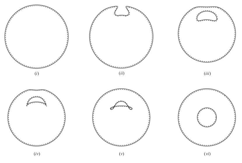
Figure 1: Qualitative depiction of the splitting process. The process necessarily involves both splitting and flipping.

Applying the approach described in section 3, our goal is to construct a solution, $\phi(\bm{z})$, to the Laplace equation such that the associated equipotential surfaces reproduce the qualitative behaviour shown in figure 1.

The crucial feature of any splitting process, which emerges from the qualitative arguments we presented above, is the fact that necessarily there exists a finite interval of values of the potential for which the equipotential surfaces are self-intersecting. Such a behaviour is not compatible with the potential $\phi(\bm{z})$ being a solution to the Laplace equation in the ordinary $\mathbbm{R}^{3}$ space, because the associated gradient, $\bm{\nabla}\phi(\bm{z})$, would be ill-defined, since the normal direction differs on the two portions of a self-intersecting equipotential surface. In the case of the intersections occurring during the flipping of the membrane orientation, this issue arises not just at isolated singular points, but over a finite region corresponding to an interval of values of $\phi(\bm{z})$. This motivates us to consider multi-valued potential functions.

More concretely the above observations lead us to propose that the potential relevant for the representation of a membrane splitting process should be a solution to the Laplace equation in a space, which we refer to as a Riemann space, that is a three-dimensional generalisation of a two-sheeted Riemann surface. Such a space consists of two copies of $\mathbbm{R}^{3}$ connected by a branch surface, bounded by a branch curve or loop. For simplicity we will assume the surface connecting the two $\mathbbm{R}^{3}$’s to always have the topology of a disk and in the following we will use the expression branch disk without necessarily implying a circular planar shape . Deformations of the branch disk which leave the branch loop fixed yield physically equivalent Riemann spaces. This is analogous to properties of branch cuts and branch points of Riemann surfaces. A space defined in this way is locally equivalent to $\mathbbm{R}^{3}$, but differs globally. The use of a Riemann space makes it possible to have a potential which locally solves the Laplace equation, while avoiding the problems caused by self-intersecting equipotential surfaces. The solution is such that different portions of self-intersecting surfaces live on different sheets of the Riemann space, so that no intersections take place within the same copy of $\mathbbm{R}^{3}$.

The description of a stable spherical membrane in section 4.1 provides an indication of what the asymptotic behaviour of the potential should be in the case of a splitting process. The infinite past, $t\to-\infty$, corresponds to $s\to+\infty$, i.e. large values of the potential. In this region the equipotential surfaces should be small spheres with radius proportional to $J$ and approaching zero. The infinite future, $t\to+\infty$, corresponds to $s\to 0$, i.e. small values of the potential approaching zero from above. In this region the equipotential surfaces should be two large concentric spheres with radii proportional to $J_{1}$ and $J_{2}$ and growing indefinitely. Using a Riemann space we can construct a potential which provides a concrete realisation of this type of asymptotic behaviour and is also well-defined in the intermediate region where the membranes self-intersect. More precisely, in order to account for the behaviour at large $\phi$ we consider a point charge $J$ at the origin of the first $\mathbbm{R}^{3}$, so that close to the charge we have a Coulomb potential, whose equipotential surfaces are small spheres. The behaviour in the two $\mathbbm{R}^{3}$’s for small $s$, on the other hand, can be understood as resulting from the splitting of the initial flux $J$ of $\bm{\nabla}\phi$, with a fraction $J_{1}$ going to infinity in the first space and a fraction $J_{2}=J-J_{1}$ passing into the second space through the branch disk.

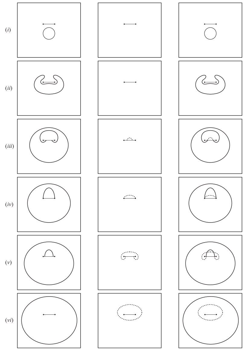
Figure 2: Qualitative depiction of splitting in Riemann space.

Figure 2 illustrates qualitatively the splitting process as rendered in the Riemann space, with the six rows in the picture corresponding to the same stages of the splitting process shown in figure 1. The first two columns depict the two sheets of the Riemann space, with each copy of $\mathbbm{R}^{3}$ represented as a rectangle. The horizontal slit corresponds to the branch disk, with the dots at the end points indicating the branch loop. The third column shows the two copies of $\mathbbm{R}^{3}$ superposed. Membranes, or portions of membranes, are represented as continuous lines in the first $\mathbbm{R}^{3}$ and as dashed lines in the second $\mathbbm{R}^{3}$. The same notation will be used in the figures throughout the paper. Re-analysing the splitting process as presented in the figure allows us to clarify how the issues associated with the flipping of the membrane orientation and the self-intersections in the equipotential surfaces can be addressed using a Riemann space. As the value of the potential decreases, away from the point charge, the equipotential surfaces intersect the branch disk and therefore extend partially into the second copy of $\mathbbm{R}^{3}$. This is shown at step ($iii$), where the splitting has already taken place. Crucially the use of a Riemann space allows us to have self-intersecting surfaces which result from the superposition of portions of surfaces without self-intersections in each sheet. This is illustrated in row ($v$) in figure 2. Notice that in the third column intersections occur only between a continuous and a dashed line, never between two continuous or two dashed lines. The final configuration in the splitting process is represented by two membranes, each contained entirely in one copy of $\mathbbm{R}^{3}$, with the superposition resulting in two concentric surfaces.

As already pointed out, a feature of the solution is that during the flipping process the equipotential surfaces develop cusps. These special points occur as the equipotential surfaces intersect the branch loop, as shown at step ($iv$) in figure 2. From the explicit solutions discussed in the next subsection one can verify that the potential itself is regular over the entire Riemann space (except for the origin of the first $\mathbbm{R}^{3}$ where the point charge is located), including the branch loop where the cusps arise . At these points, however, the gradient of the potential diverges. This allows us to physically characterise the branch loop in the Riemann space in terms of the behaviour of the solution to the continuum Nahm equations. Recalling that the potential, $s=\phi(\bm{z})$, is obtained inverting the functions $z^{i}(s)$, we deduce that the branch loop, where $\bm{\nabla}\phi(\bm{z})$ diverges, corresponds to points where the velocity of the front of the membrane, as described by $z^{i}(s)$ in Euclidean time, vanishes.

Various other properties of the instanton solutions corresponding to membrane splitting processes and their moduli spaces can be given an intuitive interpretation using a description in terms of Riemann spaces. We will discuss some of these aspects in section 4.3.2.

4.2.2 Analytic solution

In section 3 we have shown that the problem of solving the continuous version of the instanton equations can be mapped to that of finding solutions to the three-dimensional Laplace equation. Then in the previous subsection we have discussed the boundary conditions that we propose to consider in order to obtain a potential with the required properties. We now present analytic examples showing explicitly that solutions obeying such boundary conditions can be constructed.

Based on the examples of static solutions presented in section 4.1, we expect the potential for large $s$ (corresponding to $t\to-\infty$ in the original Euclidean time variable) to have a Coulomb-like singularity. The considerations in the previous subsection about the expected qualitative behaviour of the potential then lead us to consider the Laplace equation in a Riemann space made of two copies of $\mathbbm{R}^{3}$, with boundary conditions associated with the presence of a single positive point charge at the origin of the first $\mathbbm{R}^{3}$.

The idea of studying the Laplace equation in a Riemann space has actually been considered long ago by Sommerfeld in a 1896 paper [23], which introduces the idea of Riemann spaces to develop a generalisation of the standard method of images for the solution of electrostatics problems. The examples studied in [23] involve multiple copies of $\mathbbm{R}^{3}$ with branch curves consisting of straight lines. Following Sommerfeld’s proposal, an analytic solution to the Laplace equation with boundary conditions precisely of the type we are interested in was constructed by Hobson in [29]. This paper considers a Riemann space consisting of two copies of $\mathbbm{R}^{3}$ connected by a flat circular branch disk and computes the potential generated by a point charge located in the first $\mathbbm{R}^{3}$. More recently, Riemann spaces have been considered in [30, 31]. It can be shown that Sommerfeld’s solution with a straight branch line and Hobson’s solution with a circular branch loop can be related by an inversion transformation, see appendix D.

Hobson’s solution is written in terms of so-called peripolar coordinates, which are particularly suited to the specific geometry under consideration. The peripolar coordinates of a point $P$ are designated by $(\rho,\theta,\varphi)$. Their definition in $\mathbbm{R}^{3}$ and their relation to the Cartesian coordinates, $(z^{1},z^{2},z^{3})$, can be given as follows. One starts with a circle of radius $a$, which will later be identified with the branch loop and we conventionally take to lie in the $(z^{1},z^{2})$ plane. A plane containing the point $P$ and the axis of the circle, which we identify with the $z^{3}$ axis, intersects the circle at two diametrically opposite points, $A$ and $B$. Denoting the distances of $P$ from $A$ and $B$ respectively by $r$ and $r^{\prime}$, the coordinate $\rho$ of $P$ is defined as

$$\rho=\log\frac{r}{r^{\prime}}\,,$$ (4.9)

while $\theta$ is the $\widehat{APB}$ angle. The angle $\varphi$ is the standard polar angle for the projection, $N$, of $P$ onto the $(z^{1},z^{2})$ plane. Figure 3 illustrates the definition of $\rho$, $\theta$ and $\varphi$ and their relation to the Cartesian coordinates.

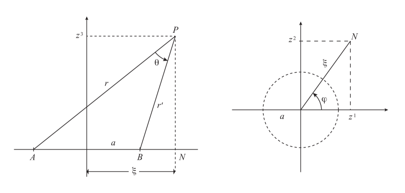
Figure 3: Relation between peripolar and Cartesian coordinates

The angle $\varphi$ is taken to vary between $0$ and $2\pi$. From the definition $\rho\in(-\infty,+\infty)$ and $\theta$ is defined to be in the interval $[-\pi,+\pi]$. The angle $\theta$ goes to $0$ when the distance of $P$ from the origin goes to $\infty$ and in the region of the $(z^{1},z^{2})$ plane outside the circle. It has a discontinuity as one passes through the interior of the disk bounded by the circle of radius $a$. It approaches $+\pi$ or $-\pi$ if one approaches a point inside the disk from above ($z^{3}>0$) or below ($z^{3}<0$) respectively. Points on the $z^{3}$ axis correspond to $\rho=0$ and points on the circle of radius $a$ in the $(z^{1},z^{2})$ plane have $\rho=\pm\infty$.

Denoting by $\xi$ the distance of the point $N$ from the origin, the peripolar and Cartesian coordinates are related by

$$z^{1}=\xi\cos\varphi\,,\quad z^{2}=\xi\sin\varphi\,,\quad z^{3}=\frac{a\sin\theta}{\cosh\rho-\cos\theta}\,,$$ (4.10)

where

$$\xi=\frac{a\sinh\rho}{\cosh\rho-\cos\theta}\,.$$ (4.11)

To describe (in peripolar coordinates) a Riemann space consisting of two copies of $\mathbbm{R}^{3}$ connected by a branch disk coinciding with the disk bounded by the circle of radius $a$ in the $(z^{1},z^{2})$ plane, one simply allows the range of $\theta$ to extend from $-\pi$ to $3\pi$. The intervals $[-\pi,\pi]$ and $[\pi,3\pi]$ correspond to the first and second $\mathbbm{R}^{3}$ respectively. Moving in the first $\mathbbm{R}^{3}$ from infinity towards the origin along the positive $z^{3}$ axis (or any other curve in the $z^{3}>0$ region) $\theta$ is positive and increases from $0$ to $\pi$. Crossing the disk at $z^{3}=0$, one crosses into the second $\mathbbm{R}^{3}$, while $\theta$ varies continuously. Moving along the negative $z^{3}$ away from the origin in the second space, $\theta$ continues to increase from $\pi$, reaching $2\pi$ as $z^{3}\to-\infty$. Approaching the origin along the positive $z^{3}$ axis in the second space the angle $\theta$ varies from $2\pi$ to $3\pi$, which is reached on the upper side of the disk. Passing through the disk one crosses back into the first space (with $z^{3}<0$) and $\theta$ goes back to $-\pi$.

The Laplacian in peripolar coordinates takes the form

$$\bm{\nabla}^{2}= \left(\frac{\cosh\rho-\cos\theta}{a^{2}}\right)\left[(\cosh\rho-\cos\theta)\frac{\partial^{2}}{\partial\rho^{2}}+\frac{(1-\cos\theta\cosh\rho)}{\sinh\rho}\frac{\partial}{\partial\rho}\right.$$

$$\left.+(\cosh\rho-\cos\theta)\frac{\partial^{2}}{\partial\theta^{2}}-\sin\theta\frac{\partial}{\partial\theta}+\frac{(\cosh\rho-\cos\theta)}{\sinh^{2}\rho}\frac{\partial^{2}}{\partial\varphi^{2}}\right]\,.$$ (4.12)

In [29] Hobson computed the potential solving the Laplace equation in the two-sheeted Riemann space with a circular branch loop for an arbitrary relative position of the point charge in the first space relative to the branch disk. Denoting by $\bm{z}_{0}$ the location of the point charge, with peripolar coordinates $(\rho_{0},\theta_{0},\varphi_{0})$, the potential at a generic point $\bm{z}$ of coordinates $(\rho,\theta,\varphi)$ is

$$\phi(\bm{z},\bm{z}_{0})=\frac{J}{4\pi|\bm{z}-\bm{z}_{0}|}\left[\frac{1}{2}+\frac{1}{\pi}\arcsin\!\left(\cos\left(\frac{\theta-\theta_{0}}{2}\right)\sqrt{\frac{2}{\cosh\alpha+1}}\right)\right]\,,$$ (4.13)

where

$$\cosh\alpha=\cosh\rho\cosh\rho_{0}-\cos(\varphi-\varphi_{0})\sinh\rho\sinh\rho_{0}$$ (4.14)

and

$$|\bm{z}-\bm{z}_{0}|=a\sqrt{2}\sqrt{\frac{\cosh\alpha-\cos(\theta-\theta_{0})}{(\cosh\rho-\cos\theta)(\cosh\rho_{0}-\cos\theta_{0})}}\,.$$ (4.15)

Notice that the potential (4.13) is periodic in $\theta$ with period $4\pi$, as appropriate for the two-sheeted Riemann space. One can verify that $\phi(\bm{z},\bm{z}_{0})$ is well-defined and finite everywhere, including the branch loop, except for the location of the point charge, i.e. $\bm{z}=\bm{z}_{0}$ in the first space, where it has a Coulomb-like divergence.

As anticipated in the previous subsection, the flux of $\bm{\nabla}\phi$ provides a measure of the angular momentum carried by the different membranes, which is also proportional to their respective radius. In the case under consideration we have a two-sheeted Riemann space with one point charge in the first copy of $\mathbbm{R}^{3}$. We will see that the equipotential surfaces for large values of the potential are small spheres centred at the location of the point charge. They represent the single membrane with angular momentum $J$ at large negative values of the original Euclidean time $t$. The flux of $\bm{\nabla}\phi$ through these surfaces is $J$. The asymptotic equipotential surfaces for small values of the potential approaching zero will be shown to be two (approximately) concentric spheres with diverging radii, one in each copy of $\mathbbm{R}^{3}$. The flux of $\bm{\nabla}\phi$ through these spheres (coinciding with the flux at infinity in the respective $\mathbbm{R}^{3}$) equals the angular momentum of the corresponding membrane, $J_{i}$, $i=1,2$. Conservation of the flux, which corresponds to conservation of angular momentum for the membranes, implies $J=J_{1}+J_{2}$. The way in which the flux $J$ is split between the two spaces is controlled by the size of the branch disk and by its position relative to the point charge. For a disk of given radius, if the point charge is located very far from the disk only a small fraction of the flux passes through the disk into the second space and thus we have $J_{2}\ll J_{1}$, corresponding to a final state with one membrane much larger than the other. If we reduce the distance between the point charge and the branch disk, the fraction of flux passing into the second space increases. When the distance of the charge from the disk tends to zero, we approach the case in which the flux is equally spit between the two spaces, which in turn corresponds to having two membranes of equal radius in the final state.

These general considerations can be made more precise by studying the asymptotic behaviour of $\phi(\bm{z},\bm{z}_{0})$ at a large distance from both the point charge and the branch disk in each of the two spaces. For this purpose we analyse $\phi(\bm{z},\bm{z}_{0})$ in the region defined by $\rho\rightarrow 0$, $\theta\rightarrow 0$ in the first space and $\rho\rightarrow 0$, $\theta\rightarrow 2\pi$ in the second space. In both cases we have $\cosh\alpha\approx\cosh\rho_{0}$. The asymptotic behaviour at infinity in the first space is

$$\phi(\bm{z},\bm{z}_{0})\approx\frac{J}{4\pi|\bm{z}-\bm{z}_{0}|}\left[\frac{1}{2}+\frac{1}{\pi}\arcsin\left(\frac{\cos\left(\frac{\theta_{0}}{2}\right)}{\cosh\left(\frac{\rho_{0}}{2}\right)}\right)\right]$$ (4.16)

and in the second space it is

$$\phi(\bm{z},\bm{z}_{0})\approx\frac{J}{4\pi|\bm{z}-\bm{z}_{0}|}\left[\frac{1}{2}-\frac{1}{\pi}\arcsin\left(\frac{\cos\left(\frac{\theta_{0}}{2}\right)}{\cosh\left(\frac{\rho_{0}}{2}\right)}\right)\right].$$ (4.17)

The factors in square brackets in (4.16) and (4.17), multiplying the Coulomb potential $J/(4\pi|\bm{z}-\bm{z}_{0}|)$, represent the fractions of the total flux staying in the first space or escaping into the second space, respectively. They determine the angular momenta $J_{1}$ and $J_{2}$ of the two membranes in the final state as fractions of the total angular momentum $J$.

In the axially symmetric case in which the point charge is located on the axis of the branch disk, corresponding to $\rho_{0}=0$, the asymptotic formulae (4.16) and (4.17) simplify and we get

$$\phi(\bm{z},\bm{z}_{0})\approx\frac{J}{4\pi|\bm{z}-\bm{z}_{0}|}\left(1-\frac{|\theta_{0}|}{2\pi}\right),$$ (4.18)

in the first space and

$$\phi(\bm{z},\bm{z}_{0})\approx\frac{J}{4\pi|\bm{z}-\bm{z}_{0}|}\frac{|\theta_{0}|}{2\pi},$$ (4.19)

in the second space. Notice that for $\theta_{0}\to\pm\pi$, i.e. when the location of the point charge approaches the disk, the ratio goes to $1/2$ as it should be.

In the following we set $a=1$ and we present plots of the equipotential surfaces of the potential (4.13) in the axially symmetric case, $\rho_{0}=0$. We can also set $\varphi_{0}=0$ without loss of generality, so that the only remaining parameter in the solution is the angle $\theta_{0}$, whose value controls the distance of the branch loop from the point charge . As will be shown in the explicit examples below, the value of $\theta_{0}$ also affects the order in which the splitting and flipping of the membrane orientation take place. Therefore the sequence in which these steps occur is correlated with the way the angular momentum gets divided between the two membranes in the final state.

Using the relations (4.10)-(4.11) in (4.13), one can obtain the form of the potential in Cartesian coordinates, $\phi=\phi(z^{1},z^{2},z^{3})$, which is the expression used to produce the plots presented below. In all the following figures we use a rescaled potential, $\hat{\phi}$, related to (4.13) by $\hat{\phi}=(4\pi/J)\phi$.

In figure 4 we show contour plots for the potential (4.13) with $\theta_{0}=-4\pi/5$. The figure shows families of equipotential surfaces separately in the two copies of $\mathbbm{R}^{3}$. Each $\mathbbm{R}^{3}$ is represented by a square, with the vertical direction being the direction of the $z^{3}$ axis. The branch disk is indicated by a horizontal slit, the point charge (contained in the first $\mathbbm{R}^{3}$, which is on the left) is denoted by a small crossed circle below the disk. The contours are displayed as continuous lines in the first space and as dashed lines in the second space.

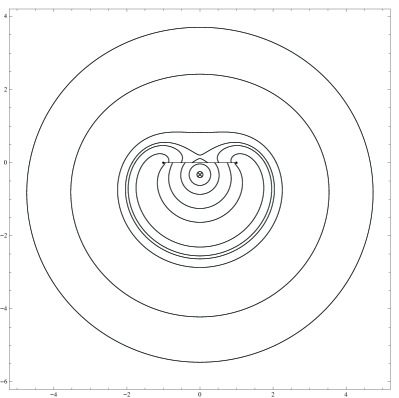
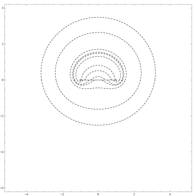
Figure 4: Contour plots showing families of equipotential surfaces in each of the two copies of $\mathbbm{R}^{3}$ which constitute the Riemann space. The contours shown are for $\theta_{0}=-\frac{4\pi}{5}$ and correspond to unequally spaced values of $\hat{\phi}$. The values of the potential used here are $\hat{\phi}=\{3.113,1.613,0.878,0.593,0.368,0.323,0.310,0.278,0.173,0.128\}$ and include those used in figure 5.

The following figures depict the evolution of the profile of the membranes throughout the splitting process for different values of $\theta_{0}$. They show how the equipotential surfaces for the potential in the analytic solution (4.13) reproduce the steps that were qualitatively discussed in the previous subsection. In these figures the two copies of $\mathbbm{R}^{3}$ are superposed. The (portions of) membranes living in the first or second space are depicted as continuous or dashed lines respectively. The figures display axially symmetric solutions, therefore the three-dimensional shape of the membranes can be generated rotating the contours about the vertical axis.

It is interesting to notice that the equipotential surfaces deviate significantly from a spherical shape only for a rather small range of the potential around the value where the splitting takes place. This is the region in which the equipotential surfaces cross the branch disk. The surfaces then quickly revert to Coulomb-like behaviour outside this region for both larger and smaller values of $\hat{\phi}$.

Figure 5 shows the membrane profiles corresponding to the choice $\theta_{0}=-4\pi/5$ in (4.13). In this case the point charge is quite close to the branch disk and correspondingly the flux/angular momentum gets split almost evenly between the two spaces. The sequence of plots shows the formation of cusps, which in these examples with axial symmetry occur simultaneously at all points on the branch loop. The membrane is then seen self-intersecting before it splits into two. As a result, with this choice of boundary conditions when the splitting occurs the second membrane has already the correct orientation, but the two membranes are still intersecting. Notice that, as anticipated in the qualitative description of the previous subsection, all the intersections between equipotential surfaces in the figure (in the third, fourth and fifth panel) involve a dashed and a continuous line, i.e. they always occur between (portions of) equipotential surfaces belonging to different sheets of the Riemann space. The same feature can be observed in all the subsequent figures in this and the next subsection.

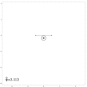
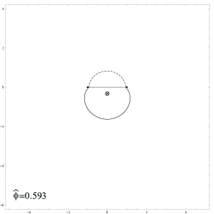
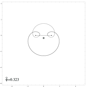
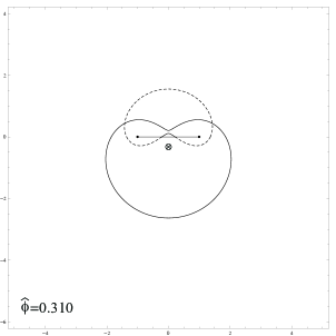
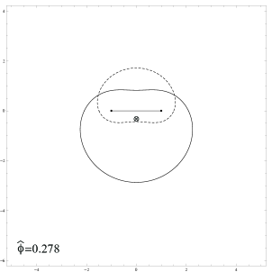
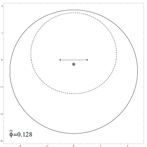
Figure 5: Evolution of the membrane profiles, showing the different phases of the splitting process in Euclidean time in the case $\theta_{0}=-4\pi/5$

Figure 6 shows the evolution of the membrane profiles for $\theta_{0}=-\pi/6$, which corresponds to a point charge much further from the branch disk. In this case the splitting process follows a sequence of steps similar to those depicted qualitatively in figures 1 and 2. The initial membrane splits into a membrane and an anti-membrane, which subsequently flips its orientation. The cusps are formed after the splitting and the subsequent flipping of the orientation of the internal membrane requires the latter to self-intersect. This takes place in the fifth panel in the figure and is shown more clearly in figure 7, which shows an enlargement of the rectangular area marked in figure 6. This example shows a concrete realisation, in an exact analytic solution, of the crucial step – illustrated at stage ($v$) in figures 1 and 2 – which led us to the concept of Riemann space. Notice the relative size of the two membranes in the final state; in this case (with the point charge further away from the disk) the flux is split less evenly than in the previous case and correspondingly the second membrane is much smaller.

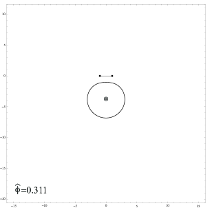
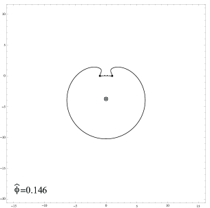
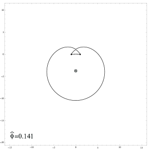
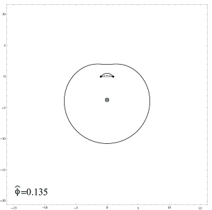
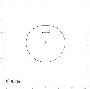
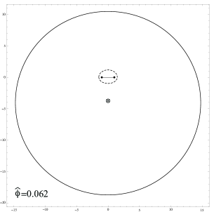
Figure 6: Evolution of the membrane profiles, showing the different phases of the splitting process in Euclidean time in the case $\theta_{0}=-\pi/6$

Figure 7: Enlargement of the area marked by a rectangle in the fifth panel of figure 6.

Figure 8 shows the splitting process for $\theta_{0}=-\pi/3$, i.e. a value intermediate between the cases shown in the previous two figures. In this case the splitting and flipping phases occur simultaneously. At the splitting point the second membrane is still self-intersecting and its orientation not completely flipped. The relative size of the two membranes in the final state reflects the fact that in this case the value of $\theta_{0}$ (which controls the distance between point charge and branch disk) is intermediate between those in the two previous examples. It corresponds to a splitting of the flux/angular momentum $J$ into $J_{1}$ and $J_{2}$ such that the difference $|J_{1}-J_{2}|$ is larger than in the first case and smaller than in the second case.

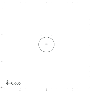
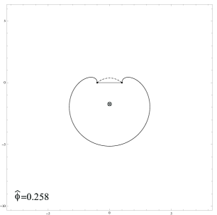
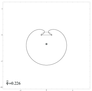
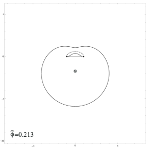
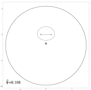
Figure 8: Evolution of the membrane profiles, showing the different phases of the splitting process in Euclidean time in the case $\theta_{0}=-\pi/3$

If the point charge is not located on the axis of the disk the qualitative behaviour of the solutions and the associated equipotential surfaces remains the same. The processes display similar sequences of steps involving splitting and flipping. In this case, however, the cusp singularities where $\bm{\nabla}\phi$ diverges do not form simultaneously on the whole branch loop, but rather at pairs of points.

The equipotential surfaces for the potential (4.13), once expressed in Cartesian coordinates, represent implicit equations of the membrane profiles as described by the $z^{i}(s)$ variables. The evolution of the shape of the membranes during a splitting process in terms of the original coordinates, $y^{i}(t)$, can be reconstructed using the change of variables (3.7) in the potential $\phi(z^{1},z^{2},z^{3})$ . The qualitative features of the equipotential surfaces parameterised by the $y^{i}$ coordinates are similar. The only significant difference is that the size of the membranes does not grow steadily as seen in the previous figures. This is the same difference that was observed in section 4.1 in the case of the description of the static spherical solution in terms of the $y^{i}$ and $z^{i}$ variables. Using the $y^{i}$ variables one can instead verify immediately that the solutions describe a process in which the final membranes have radii which add up to the radius of the single membrane in the initial state. In the next subsection we will present plots showing the evolution of the membrane profiles, using the parametrisation in terms of the $y^{i}$ variables, in the case of solutions interpolating between configurations with two membranes in the initial state and two in the final state.

4.3 General Riemann spaces

In the previous subsections we presented explicit solutions to the Laplace equation describing the most elementary splitting process with a single membrane in the initial state and two membranes in the final state. It is natural to ask whether a similar approach can be used to construct other solutions corresponding to (anti-)instantons of the pp-wave matrix model interpolating between states with different numbers of membranes. A large class of solutions connecting multi-membrane states was shown to exist in [18]. For our reformulation in terms of the Laplace equation to be equivalent to the original (continuum) instanton equations, solutions should exist for all the allowed instanton configurations. Therefore it should be possible to identify suitable boundary conditions corresponding to all the pairs of initial and final states for the original equations, which are permitted according to the criteria in [18]. Indeed, we will show that the conditions for the existence of BPS instanton solutions obtained in [18] can be reproduced using our formulation in terms of the Laplace equation in a Riemann space.

An analysis of the general features of the solutions we discussed above provides hints for the generalisation to more complicated processes. In the cases discussed in section 4.2 the two membranes in the final state correspond to equipotential surfaces in the asymptotic regions at infinity, one in each of the two copies of $\mathbbm{R}^{3}$ constituting the Riemann space. On the other hand the single membrane in the infinite past corresponds to small spheres centred at the location of the point charge. These considerations lead us to propose the following general prescription. In order to describe a process with $n$ membranes in the final state one should consider a Riemann space made of $n$ copies of $\mathbbm{R}^{3}$. Moreover, if the initial state contains $m$ membranes one should consider $m$ (positive) point charges at the origin of $m$ distinct $\mathbbm{R}^{3}$’s. The values of the point charges, $J_{i}$, $i=1,2,\ldots,m$, correspond to the angular momenta of the $m$ membranes in the initial state. The values of the flux of $\bm{\nabla}\phi$ at infinity in each copy of $\mathbbm{R}^{3}$, $J_{i}^{\prime}$, $i=1,2,\ldots,n$, correspond to the angular momenta of the $n$ membranes in the final state. We point out that an immediate consequence of this prescription is that by construction the number, $n$, of membranes in the final state is greater than or equal to the number, $m$, of membranes in the initial state. Therefore the necessary condition, $n\geq m$, for the existence of instanton solutions is automatically satisfied.

In the case of a generic Riemann space the relation between the outgoing fluxes at infinity, $J^{\prime}_{i}$, and the values of the point charges at the origin, $J_{i}$, is non-trivial. This is because the way in which the flux of $\bm{\nabla}\phi$ gets split among the different spaces depends in a complicated way on the number, shape and size of the branch disks and on their positions relative to the point charges. In the most elementary case of the solution (4.13) we gave explicit formulae for the asymptotic fluxes associated with the two membranes in the final state in (4.16)-(4.19).

General multi-sheeted Riemann spaces can involve different combinations of branch surfaces. This is the case even in the most elementary example discussed in the previous subsection, in which one membrane with angular momentum $J$ splits into two membranes with angular momenta $J_{1}$ and $J_{2}$. We described this process using a Riemann space made of two copies of $\mathbbm{R}^{3}$ with a single point charge, $J$, and we presented an exact solution involving a circular branch disk. However, the same process receives contributions from more complicated Riemann spaces in which the two $\mathbbm{R}^{3}$’s are connected by multiple branch disks, so long as the flux at infinity in the two spaces is split into the same fractions, $J_{1}$ and $J_{2}$. Of course in order to compute a specific physical transition amplitude it is necessary to sum all the contributions with the given initial and final states. The issue of how the different copies of $\mathbbm{R}^{3}$ are connected is related to the parameterisation of the moduli spaces of the associated instanton solutions and we will briefly comment on this point in section 4.3.2.

At the present stage we do not have a proof of existence of solutions to the three-dimensional Laplace equation in arbitrary Riemann spaces, but we propose as a conjecture that solutions should exist for all the boundary conditions which according to our prescription correspond to allowed (anti-)instantons. The results of [23] and [29] provide a starting point for the analysis of the issue of existence of solutions in general Riemann spaces. One may view the explicit solutions in [23] and [29] as playing a role similar to that played by the explicit solution for a spherical conductor obtained by the method of images in connection with the theory of the electric potential for arbitrarily shaped conductors. Moreover the Laplace equation in the Riemann space can be recast into the form of an integral equation as discussed in appendix E. This reformulation may also provide a useful approach to obtain a proof of existence for the solutions.

4.3.1 More solutions

Before discussing how some general properties of the instanton moduli space arise within our formulation using the Laplace equation, we now present other exact solutions. We use these specific examples to illustrate some interesting features arising more generally in the description of instanton configurations in terms of equipotential surfaces.

The linearity of the Laplace equation of course implies that linear combinations of solutions are also solutions. We can take advantage of this simple observation to obtain new interesting examples. In particular, a solution describing a process with two membranes with angular momenta $J_{1}$ and $J_{2}$ in the initial state and two in the final state – which based on our prescription requires a two-sheeted Riemann space with a point charge in each copy of $\mathbbm{R}^{3}$ – can be obtained as a linear combination of the potential (4.13) with charge $J_{1}$ and the analogous potential with point charge $J_{2}$ at $\bm{z}=\bm{z_{0}}$ in the second space. To obtain the potential due to a point charge at the point corresponding to $\bm{z}_{0}$ in the second space, we recall that in peripolar coordinates the first sheet is parameterised by $\theta\in[-\pi,\pi]$ and the second sheet by $\theta\in[\pi,3\pi]$. Therefore the potential induced by a charge located at the point in the second $\mathbbm{R}^{3}$ corresponding to $\bm{z}_{0}$ is obtained substituting $\theta_{0}\to\theta_{0}+2\pi$ in (4.13). The resulting solution in the two sheeted Riemann space with point charges in both spaces is

$$\phi(\bm{z},\bm{z}_{0}) =\frac{J_{1}}{4\pi|\bm{z}-\bm{z}_{0}|}\left[\frac{1}{2}+\frac{1}{\pi}\arcsin\!\left(\cos\left(\frac{\theta-\theta_{0}}{2}\right)\sqrt{\frac{2}{\cosh\alpha+1}}\right)\right]$$

$$\,+\frac{J_{2}}{4\pi|\bm{z}-\bm{z}_{0}|}\left[\frac{1}{2}-\frac{1}{\pi}\arcsin\!\left(\cos\left(\frac{\theta-\theta_{0}}{2}\right)\sqrt{\frac{2}{\cosh\alpha+1}}\right)\right]$$ (4.20)

$$=\frac{1}{4\pi|\bm{z}-\bm{z}_{0}|}\left[\frac{(J_{1}+J_{2})}{2}+\frac{(J_{1}-J_{2})}{\pi}\arcsin\!\left(\cos\left(\frac{\theta-\theta_{0}}{2}\right)\sqrt{\frac{2}{\cosh\alpha+1}}\right)\right],$$

where $|\bm{z}-\bm{z}_{0}|$ and $\cosh\alpha$ are given in (4.15) and (4.14) respectively and we have chosen the radius of the branch loop to be $a=1$. The sign difference between the first two lines in (4.20) comes from the shift in $\theta_{0}$. Recalling that $\cosh\alpha$ is independent of $\theta_{0}$, we get

$$\arcsin\!\left[\cos\left(\frac{\theta-(\theta_{0}+2\pi)}{2}\right)\sqrt{\frac{2}{\cosh\alpha+1}}\right]=-\arcsin\!\left[\cos\left(\frac{\theta-\theta_{0}}{2}\right)\sqrt{\frac{2}{\cosh\alpha+1}}\right],$$ (4.21)

because the shift by $\pi$ in the argument flips the sign of the cosine and the inverse sine function is odd. Notice that if the two charges are equal, $J_{1}=J_{2}$, (4.20) reduces to a simple Coulomb potential in both sheets of the Riemann space. This is consistent with our general prescription. With equal charges the fluxes of $\bm{\nabla}\phi$ from the first space into the second and from the second space into the first are equal, irrespective of the position, $\bm{z}_{0}$, of the charges. So the flux at infinity in the two spaces is the same and hence the final state is the same as the initial state. Therefore this case corresponds simply to a stable vacuum configuration with two membranes of the same size. Note that, up to an overall scale, the potential (4.20) can also be obtained from the superposition of the solution (4.13) and a simple Coulomb potential.

We now focus on the special case of axially symmetric solutions (corresponding to $\rho_{0}=\varphi_{0}=0$) with $J_{1}=2J$, $J_{2}=J$ for which (4.20) becomes

$$\phi(\bm{z},\bm{z}_{0})=\frac{J}{4\pi|\bm{z}-\bm{z}_{0}|}\left[\frac{3}{2}+\frac{1}{\pi}\arcsin\!\left(\cos\left(\frac{\theta-\theta_{0}}{2}\right)\sqrt{\frac{2}{\cosh\rho+1}}\right)\right]\,,$$ (4.22)

where we used the fact that $\cosh\alpha=\cosh\rho$ when $\bm{z}_{0}$ is on the axis of the disk.

The final states in the process described by the potential (4.22) depend on the way in which the total flux at infinity is divided between the two spaces, which in turn is controlled by the value of $\theta_{0}$. Different choices for $\theta_{0}$ give rise to solutions displaying various interesting features and below we present a few selected examples.

The following figures 9, 11 and 13 show the evolution of the two membranes described by the solution (4.22) for $\theta_{0}=-2\pi/3$, $\theta_{0}=-\pi/10$ and $\theta_{0}=-\pi/6$ respectively. As in the previous subsection, the plots show equipotential surfaces for the rescaled potential $\hat{\phi}=(4\pi/J)\phi$. The figures depict the equipotential surfaces for $\phi(y^{1},y^{2},y^{3})$ expressed in terms of the coordinates, $y^{i}(t)$, in the original instanton equations (3.6). The conventions used are the same as in previous figures. The (portions of) membranes in the first copy of $\mathbbm{R}^{3}$ are shown as continuous contours and those in the second $\mathbbm{R}^{3}$ as dashed contours. Since here we are using the $y^{i}$ coordinates, the contours represent the evolution of the profiles of the membranes from $t=-\infty$ to $t=+\infty$. Notice that with this parameterisation of the solution the membranes do not expand steadily. However, their relative radii change between the initial and final state because of the transfer of angular momentum. The use of these variables makes manifest the conservation of angular momentum ($J_{1}^{\prime}+J_{2}^{\prime}=J_{1}+J_{2}$), which in the figures is reflected in the fact that the radii of the spheres in the initial and final states add up to the same total. In the figures we have not displayed the branch loop as in these coordinates its position is not constant.

In the case shown in figure 9 the value of $\theta_{0}=-2\pi/3$ and thus the point charges are relatively close to the branch disk. As a result there is a large fraction of flux passing from the first $\mathbbm{R}^{3}$ into the second. This corresponds to a large transfer of angular momentum and thus a significant change in the relative radii of the two membranes. In the sequence shown in the figure the second and third steps show both membranes extending across both spaces. In the third panel the outer membrane develops a self-intersection. The small region marked by a square is shown enlarged in figure 10, where the self-intersection is more clearly visible. The membranes then split and reconnect in the way shown in the fourth panel of figure 9 resulting in two equipotential surfaces each contained entirely in one copy of $\mathbbm{R}^{3}$.

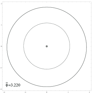
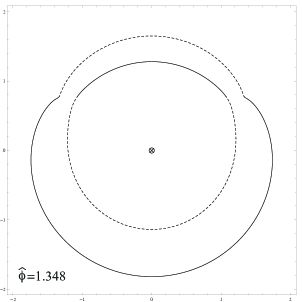
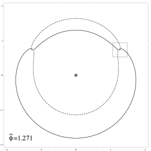
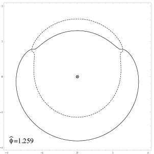
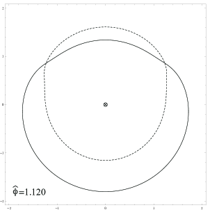
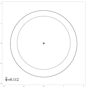
Figure 9: Evolution of the membrane profiles for a process with two membranes in the initial state and two in the final state ($\theta_{0}=-2\pi/3$).

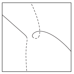
Figure 10: Enlargement of the area marked by a square in the third panel of figure 9.

In the case shown in figure 11 the point charges are at $\theta_{0}=-\pi/10$, i.e. further from the branch disk and this means that there is a smaller transfer of angular momentum. With this choice of boundary conditions we observe another interesting feature: for some intermediate values of Euclidean time there are three membranes involved in the process. A small membrane detaches from the larger membrane in the first $\mathbbm{R}^{3}$ and subsequently gets absorbed by the other membrane. In the intermediate steps this third membrane crosses the branch disk from the first $\mathbbm{R}^{3}$ into the second, flipping its orientation. The self-intersection involved in the flipping of the membrane orientation is shown in figure 12, which is an enlargement of the small rectangle marked in the fourth panel of figure 11.

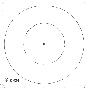
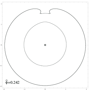
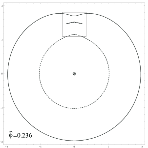
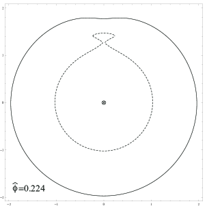
Figure 11: Evolution of the membrane profiles for a process with two membranes in the initial state and two in the final state ($\theta_{0}=-\pi/10$).

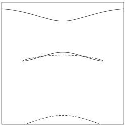
Figure 12: Enlargement of the area marked by a rectangle in the fourth panel of figure 11.

Figure 13 depicts a case intermediate between the previous two examples, corresponding to $\theta_{0}=-\pi/6$. In this case the transfer of angular momentum does not involve the exchange of a third membrane, but the interplay between the equipotential surfaces is rather interesting. In figure 14 we show a detailed view of the area within the rectangles marked in the third and fourth panels in figure 13, presenting a sequence of contour plots for values of the potential between $\hat{\phi}=0.380$ and $\hat{\phi}=0.378$. The fourth panel in figure 14 shows clearly that in this case the splitting takes place not at a point, but simultaneously at points along a ring. This is of course not a generic feature. It is a degenerate case which only occurs in axially symmetric solutions for certain values of the parameters. A similar splitting ring is also present in the previously discussed case of figure 9.

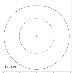
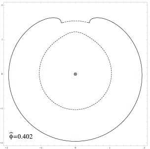
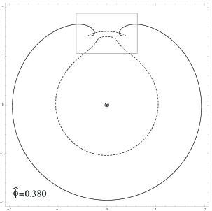
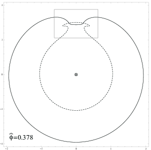
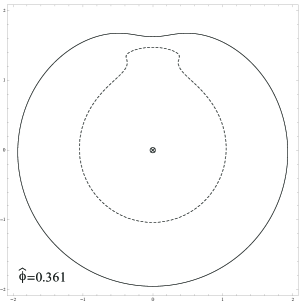
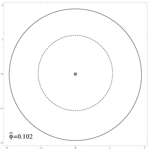
Figure 13: Evolution of the membrane profiles for a process with two membranes in the initial state and two in the final state ($\theta_{0}=-\pi/6$).

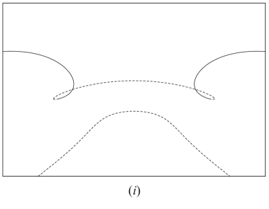
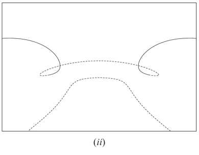
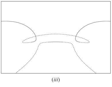
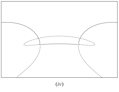
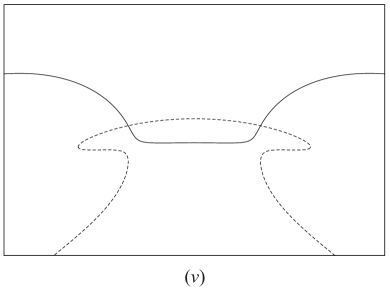
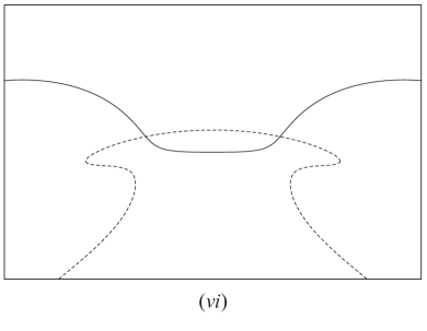
Figure 14: Enlargement of the area marked by rectangles in the third and fourth panels of figure 13, showing intermediate steps between the two.

It is quite remarkable that the rather striking behaviour of membranes illustrated by the above examples may be reproduced by solutions of such a simple and well studied equation as the Laplace equation.

4.3.2 Comments on the moduli space of solutions

In this subsection we discuss some features of the moduli space of instantons associated with general Riemman spaces. As we previously noted, the number of copies of $\mathbbm{R}^{3}$, $n$, corresponds to the number of membranes in the final state. Positive charges, $J_{i}\geq 0$ $(i=1,\ldots,n)$, can only be placed at the origin of these spaces. The charge $J_{i}$ corresponds to the angular momentum of the $i$-th membrane in the initial state. Some of the $J_{i}$’s may be zero and the number of non-zero $J_{i}$’s is the number of membranes in the initial state.

The sheets of the Riemann space are connected by branch disks, bounded by branch loops. By definition when a branch disk connects two copies of $\mathbbm{R}^{3}$ the disk is located at the same place, with the same shape, in the two copies . Except for this condition, the number of branch loops connecting the copies of $\mathbbm{R}^{3}$, their positions and their shapes are arbitrary. In the following we collectively refer to the number of copies of $\mathbbm{R}^{3}$ and the number, the positions and the shapes of the branch loops as the geometry of the Riemann space. Our conjecture is that for any geometry of the Riemann space (and the distribution of positive charges at the origins) we have a unique solution to the Laplace equation satisfying the boundary conditions.

A point on the instanton moduli space is characterised by specifying the geometry of the Riemann space. This will give an interpretation of the moduli space of solutions of the BPS instanton equation (2.12) discussed in [18] when $J$ is large (but finite). Stated differently, the moduli space associated with (2.12) can be considered as a regularisation of the moduli space of branch loops.

The outgoing flux at infinity in the $i$-th copy of $\mathbbm{R}^{3}$, which we call $J_{i}^{\prime}$, corresponds to the angular momentum of the $i$-th membrane in the final state.

A necessary and sufficient condition for the existence of solutions to the instanton equations interpolating between the initial state characterised by $J_{i}$, $i=1,\ldots,n$, and the final state characterised by $J_{i}^{\prime}$, $i=1,\ldots,n$, was established in [18]. Below we will show that the same condition can be derived from our approach taking advantage, in particular, of the linearity of the Laplace equation.

The linearity implies that for a fixed geometry of the Riemann space, one has a linear relationship between $J_{i}$ and $J_{i}^{\prime}$,

$$J_{i}^{\prime}=\sum_{j}K_{ij}J_{j}\,.$$ (4.23)

The matrix $K$ characterises the flow of the flux lines for a given Riemann space. (It is reminiscent of the coefficients of capacity in the electrostatic theory of conductors, which are determined by the shape and positions of the conductors.) In general the matrix $K$ is not symmetric. We will also use a matrix-vector notation

$$\bm{J}^{\prime}=K\bm{J}\,,$$ (4.24)

where $\bm{J}=(J_{1},\ldots,J_{n})$, $\bm{J^{\prime}}=(J^{\prime}_{1},\ldots,J^{\prime}_{n})$.

Some simple but important properties follow from the definition of $K_{ij}$. The first property is the positivity of the elements of the matrix $K$

$$K_{ij}\geq 0.$$ (4.25)

In order to see this, we consider the case in which there is only one unit charge, located at the origin of the $j$-th copy of $\mathbbm{R}^{3}$, in the entire Riemann space. The flux flowing to the $i$-th space from the $j$-th space equals $K_{ij}$. Since there is a positive charge in the $j$-th space and no charge in the $i$-th space, it is clear that the flux should always flow from the $j$-th to the $i$-th space, not the other way around. This implies $K_{ij}\geq 0$.

Other important properties of $K$ are the sum rules,

$$\sum_{i}K_{ij}=1\,\quad\forall\,j\,,$$ (4.26)

$$\sum_{j}K_{ij}=1\,\quad\forall\,i\,.$$ (4.27)

The property (4.26) simply follows from the conservation of the number of flux lines (i.e. the Laplace equation and Gauss’ theorem). The property (4.27) can be deduced as follows. We consider a special potential function in the Riemann space defined by the requirement that in each copy of $\mathbbm{R}^{3}$ it is identical to the Coulomb potential associated with a unit charge at the origin. Such a potential solves the Laplace equation and satisfies all the boundary conditions . The existence of this solution implies that if $J_{i}=(1,1,1,\ldots,1)$, then $J_{i}^{\prime}=(1,1,1,\ldots,1)$ in (4.23), which is equivalent to (4.27).

The positivity (4.25) and the sum rules (4.26)-(4.27) imply rather strong constraints on the allowed combinations of $J_{i}$’s and $J_{i}^{\prime}$’s, including conditions equivalent to the criteria given in [18] for the existence of solutions.

First, one can show that

$$\sum_{i}{J_{i}^{\prime}}^{p}\leq\sum_{i}J_{i}^{p}$$ (4.28)

for any $p\geq 1$. By using the vector norm $||\bm{v}||_{p}=(\sum_{i}|v_{i}|^{p})^{1/p}$, the matrix norm is defined by [32]

$$||A||_{p}=\underset{\bm{v}\neq 0}{\mathrm{max}}\frac{||A\bm{v}||_{p}}{||\bm{v}||_{p}}.$$ (4.29)

Hence in order to establish (4.28) it is sufficient to show

$$||K||_{p}\leq 1.$$ (4.30)

Using an inequality for matrix norms (cf. formula (1.11) in [33]),

$$||A||_{p}\leq||A||_{1}^{1/p}||A||_{\infty}^{1-1/p}$$ (4.31)

and the well-known formulae [32]

$$||A||_{1}=\underset{1\leq j\leq n}{\mathrm{max}}\sum_{i=1}^{n}|A_{ij}|,\quad||A||_{\infty}=\underset{1\leq i\leq n}{\mathrm{max}}\sum_{j=1}^{n}|A_{ij}|,$$ (4.32)

we see that $||K||_{1}=1$ and $||K||_{\infty}=1$ and hence (4.30) and (4.28) are established. For $p=3$, we have

$$\sum_{i}{J_{i}^{\prime}}^{3}\leq\sum_{i}J_{i}^{3}\,,$$ (4.33)

which gives a continuum counterpart of the necessary condition (2.16) for the existence of instantons (which can also be derived directly by defining the continuum version of (2.11)).

One can introduce an “entropy” associated with the distribution of the total angular momentum among the individual membranes defined as

$$\sum_{i}\left(-J_{i}\log J_{i}\right)\qquad{\rm and}\qquad\sum_{i}\left(-J^{\prime}_{i}\log J^{\prime}_{i}\right)$$ (4.34)

for the initial and final states respectively. Then by taking $p=1+\epsilon$ in (4.28) and using the conservation law $\sum J_{i}=\sum J^{\prime}_{i}$, one can show that the entropy is always non-decreasing,

$$\sum_{i}\left(-J^{\prime}_{i}\log{J^{\prime}_{i}}\right)\geq\sum_{i}\left(-J_{i}\log{J_{i}}\right).$$ (4.35)

Let us now deduce the necessary and sufficient condition for the existence of instantons given in [18]. The condition can be phrased as follows (cf. figure 3 in [18]). Since the $J_{i}$’s are non negative, they can be represented by a histogram as shown in figure 15 ($i$). A similar histogram can be constructed with the $J^{\prime}_{i}$’s in the final state.

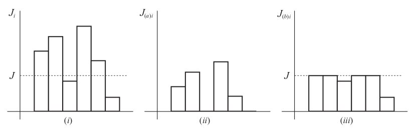
Figure 15: The angular momenta of membranes $\bm{J}=(J_{1},\ldots,J_{n})$ can be represented as a histogram as shown in ($i$). The area of the histogram $\bm{J}$ below a given height $J$ is denoted by $\mathcal{A}(J;\bm{J})$. We define histograms $\bm{J}_{(a)}$ and $\bm{J}_{(b)}$ by cutting the original histogram $\bm{J}$ along the horizontal line and taking the part above and below it, as shown in ($ii$) and ($iii$).

We draw a horizontal line at a height $J\geq 0$ on the histogram and denote the area of the histogram below the value $J$ by

$$\mathcal{A}(J;\bm{J}).$$ (4.36)

The condition in [18] can then be expressed as

$$\mathcal{A}(J;\bm{J}^{\prime})\geq\mathcal{A}(J;\bm{J})\quad\forall\,J.$$ (4.37)

(We note that we do not assume $J_{1}\geq J_{2}\geq\ldots\geq J_{n}$ or $J^{\prime}_{1}\geq J^{\prime}_{2}\geq\ldots\geq J_{n}$ here.) Thus, the area of the support of the histogram $J_{i}^{\prime}$ is always larger than or equal to that of the histogram $J_{i}$. An interpretation of this condition is that the histogram $J_{i}^{\prime}$ should be more smeared compared to the histogram $J_{i}$, which is natural in view of (4.35) .

In order to prove (4.37) we introduce two auxiliary histograms, $J_{(a)i}$ and $J_{(b)i}$, generated cutting the histogram $J_{i}$ at a fixed height $J$. As shown in figure 15, we define $J_{(a)i}$ and $J_{(b)i}$ as the histograms above and below the horizontal line at the height $J$, respectively. By definition we have

$$\bm{J}=\bm{J}_{(a)}+\bm{J}_{(b)}.$$ (4.38)

Moreover

$$\bm{J^{\prime}}=K\bm{J}=K\bm{J}_{(a)}+K\bm{J}_{(b)}.$$ (4.39)

We first focus on the histogram defined by $K\bm{J}_{(b)}$. All columns in this histogram have height smaller than or equal to $J$, i.e. $(K\bm{J}_{(b)})_{i}\leq J$. To see this we recall that (4.27) implies that

$$K\left[\begin{array}[]{c}J\\ \vdots\\ J\end{array}\right]=\left[\begin{array}[]{c}J\\ \vdots\\ J\end{array}\right].$$ (4.40)

Since all elements of $\bm{J}_{(b)}$ are smaller than or equal to $J$ by definition and all elements of $K$ are positive (4.25), the elements of $K\bm{J}_{(b)}$ cannot be larger than $J$.

The sum rule (4.26) implies that area of the histogram $K\bm{J}_{(b)}$ is the same as the area of the histogram $\bm{J}_{(b)}$, which by definition equals $\mathcal{A}(J;\bm{J})$. Now recall that $\bm{J}^{\prime}=K\bm{J}_{(a)}+K\bm{J}_{(b)}$. Since the height of the histogram $K\bm{J}_{(b)}$ is less than or equal to $J$, all of the histogram $K\bm{J}_{(b)}$ contributes to $\mathcal{A}(J;\bm{J^{\prime}})$. The area $\mathcal{A}(J;\bm{J^{\prime}})$ has a further contribution from $K\bm{J}_{(a)}$, which is always non-negative, because of the positivity of $K$ and $J_{(a)}$. Thus, we have

$$\mathcal{A}(J;\bm{J^{\prime}})\geq\mathcal{A}(J;K\bm{J}_{(b)})=\mathcal{A}(J;\bm{J}),$$ (4.41)

and (4.37) is proven.

Another interesting property of the moduli space of solutions to the BPS instanton equation (2.12), which was established in [18], is the additivity rule (2.24) for the dimension of the moduli spaces. A possible interpretation of this result, which is instructive if perhaps not mathematically rigorous, is the following. We assume that we have two instanton solutions, interpolating between vacua A and B, and between vacua B and C, such that both of them are reasonably localised in time. It is natural to expect that one can construct an instanton solution interpolating between vacuum A and vacuum C, by stitching together the two original solutions taken to be well separated in time. The number of parameters of the composite instanton thus constructed should be given by the sum of the numbers of parameters of the two original instantons.

This construction of a composite instanton from two instantons well separated in time has a natural counterpart in our description of the instantons using Riemann spaces. The following argument relies on viewing a solution in a multi-sheeted Riemann space as a composite of solutions built using pairs of connected copies of $\mathbbm{R}^{3}$. Within this picture the basic idea underlying the construction is that, at least in the asymptotic region at infinity, a branch disk with incoming flux can be viewed as a point charge. Here we wish to point out the essential features of this construction without going into the details. In the following it is crucial that the time variable in the BPS instanton corresponds to the logarithm of the distance from the origin in our description. We start with two instanton solutions, each associated with the branch disks $D_{1}$ and $D_{2}$. Because of the scale invariance of the Laplace equation, one can move one of the disks, e.g. $D_{2}$, further away from the origin by rescaling simultaneously its size and its distance from the origin. The physics associated with the second disk, such as the number of flux lines going into the disk and the profile of the potential function do not change under the rescaling. We refer to the rescaled disk as $D_{2}^{\prime}$. Now we consider a new Riemann space equipped with two branch disks, $D_{1}$ and $D_{2}^{\prime}$. Since the disk $D_{2}^{\prime}$ is sufficiently far away, its existence does not affect the potential produced by the point charge at the origin and the first branch disk $D_{1}$. Furthermore, from the viewpoint of the second disk $D_{2}^{\prime}$, the disk $D_{1}$ and the point charge appear as a new point charge at the origin whose value can be reconstructed using the original charge and the number of flux lines going through the disk $D_{1}$. In this manner, the potential on the Riemann space with two disks ($D_{1}$, $D_{2}^{\prime}$) can be constructed by using the potentials corresponding to the two separate solutions associated with the disks $D_{1}$ and $D_{2}$.

As previously mentioned, the calculation of physical transition amplitudes using a semi-classical approximation involves the integration over the collective coordinates parameterising the instanton moduli space. From the point of view of the description of the moduli space in terms of the geometry of Riemann spaces, this means that one should sum the contributions of all possible combinations of branch surfaces giving rise to the same initial and final states. Such a sum may include not only branch disks of more complicated shapes than the circular ones we discussed, but also in principle branch surfaces with more complicated topology, e.g. consisting of higher genus surfaces with boundaries. It would be interesting to study the characteristics of the resulting Riemann spaces.

5 Conclusions and discussion

In this paper we have initiated a study of the interactions associated with membrane splitting/joining processes in M-theory. We considered a large angular momentum sector of M-theory in AdS${}_{4}\times S^{7}$, which can be described using the matrix model approach in the pp-wave approximation. The vacua of the pp-wave matrix model consist of collections of concentric membranes and contributions to splitting or joining processes arise from tunnelling amplitudes between states built on vacua with different numbers of membranes. Classical tunnelling configurations are instantons, i.e. finite action solutions to the Euclidean equations of motion of the pp-wave matrix model. Relying on the same ideas underlying the definition of the matrix model as regularisation of the supermembrane theory, we have presented a method for the construction of approximate solutions to the instanton equations. Using a continuum formulation in which large matrices are approximated by functions, we have shown that the problem of constructing solutions to the instanton equations of the pp-wave matrix model can be reduced to that of solving the three-dimensional Laplace equation. A remarkable outcome of our analysis is that in order to describe membrane splitting/joining processes it is necessary to study the Laplace equation in a Riemann space, which is a three-dimensional generalisation of the familiar concept of Riemann surface. The interpolating configurations at different points in Euclidean time arise as equipotential surfaces for the solutions to the Laplace equations in a Riemann space with suitable boundary conditions. The use of Riemann spaces provides a very compelling answer to various issues arising in the description of membrane splitting processes in terms of the Laplace equation.

The approach we developed in this paper presents some similarities to the description of splitting/joining interactions in the matrix string formulation of type IIA string theory [34] in terms of instantons in two-dimensional SYM theory [35, 36, 37]. There are also some analogies between our work and [38], in which 1/4 BPS solitons in $\mathcal{N}=4$ SYM are described using multi-pronged $(p,q)$ string states. The latter are constructed using the two-dimensional Laplace equation which arises from configurations of M2-branes stretched between M5-branes.

In section 4 we presented exact solutions to the Laplace equation, which represent approximate solutions to the original BPS instanton equations valid for large $J$. The instanton configurations in the matrix model are saddle points for the Euclidean path integral of the theory and can be used to compute contributions to physical transition amplitudes using a semi-classical approximation. As a next step it will be important to deduce the exact form of the solutions in the matrix model, associated with the approximate solutions we obtained using the continuum approximation. The connection between the instanton equations and the Laplace equation in the continuum approximation is established mapping the former to the Nahm equations. This means that in the process of reconstructing the matrix model solutions we should be able to take advantage of the integrability properties of the Nahm equations.

Semi-classical contributions to physical transition amplitudes in the Lorentzian signature pp-wave matrix model should be obtained from a saddle point approximation about the instanton configurations followed by an analytic continuation. The semi-classical calculation involves an integration over the moduli space of the BPS instantons, whose properties were studied in [18, 17]. Completing the semi-classical analysis will allow us to extract effective interaction vertices for membranes in the pp-wave background. A first interesting issue to address is the determination of the associated coupling constants. Naively one would expect instanton induced transition amplitudes to be exponentially suppressed, due to the contribution of the classical instanton action. For instance the most elementary amplitude, corresponding to the splitting of a single membrane with angular momentum $J$ into two membranes with angular momenta $J_{1}$ and $J_{2}$, carries a weight

$${\rm e}^{-S_{E}}={\rm e}^{-\frac{JJ_{1}J_{2}}{8N}}\,,$$ (5.1)

where $J_{1}\sim J_{2}\sim J$ and $N^{1/3}\ll J\ll N^{1/2}$ for the applicability of the pp-wave approximation in a weak coupling regime. However, it is probably premature to conclude that the coupling constant measuring the strength of membrane interactions is exponentially small. The dependence on the parameters can be modified by factors arising from the integration over the instanton moduli space, which has a dimension that grows with $J$ – for example it is $4J_{2}$ in the case of the single membrane splitting, see (2.23). Volume factors can modify the exponential behaviour (5.1) and it is possible, at large $J$ in particular, for the complete physical transition amplitudes to have a power-law dependence on the parameters $J$ and $N$, which might be more natural from the point of view of a description of membrane interactions in target space. A similar mechanism, leading to a power-law behaviour, has been recently suggested to arise in the calculation of solitonic contributions to certain scattering amplitudes [39] and may be relevant for the understanding of the connections between the maximally supersymmetric Yang-Mills theory in five dimensions and the $(2,0)$ superconformal theory in six dimensions [40, 41].

The particular solution (2.21) constructed in [18], which approaches the configuration corresponding to the $J$-dimensional representation ${\underline{1}}\oplus{\underline{1}}\oplus\cdots\oplus{\underline{1}}$ at $t=+\infty$, was studied in the context of the pp-wave matrix model in [17]. According to a proposal presented in [42], the configuration associated with the representation ${\underline{1}}\oplus{\underline{1}}\oplus\cdots\oplus{\underline{1}}$ should be interpreted as a single M5-brane and therefore the solution (2.21) would contribute to an amplitude coupling M2- and M5-branes. It would be interesting to determine whether such a coupling has a different weight in terms of the $J$ and $N$ parameters, compared to those involving only M2-branes.

The study of instanton effects in another maximally supersymmetric theory, ${\mathcal{N}}=4$ SYM with SU($N$) gauge group, suggests that the large $J$ limit, which plays a central role in our continuum approximation, may also lead to important simplifications in the semi-classical calculation of physical transition amplitudes. In the case of ${\mathcal{N}}=4$ SYM at large $N$ the integration over the multi-instanton moduli space is dominated by special configurations and a saddle point approximation makes it possible to compute the leading contributions at large $N$ for arbitrary instanton number [43]. It would be very interesting to understand if a similar saddle point based approach can be applied in the present case for large $J$.

The following considerations, albeit somewhat speculative, may provide insights into possible mechanisms leading to the emergence of a saddle point approximation for large $J$. Among the collective coordinates parameterising the instanton moduli space there are variables associated with the SU($J$) gauge orientations, which are the remnant in the matrix model of the invariance of the membrane theory under area preserving diffeomorphisms (APD’s). When computing contributions to gauge invariant observables the integrations over these colour-related variables can be carried out and in general produce a non-trivial measure for the integrals over the remaining collective coordinates, that can be referred to as the ‘physical’ ones. At large $J$ this measure can be very peaked and give a large weight to special regions of the physical moduli space. In such a situation it is possible to expect the emergence of a good saddle point approximation. Given the fact that the SU($J$) gauge symmetry descends from the APD invariance in the continuum, it may be natural to expect that the configurations acquiring the largest weight in the physical moduli space should be the smoothest ones, since they are the ones for which the finite SU($J$) symmetry is closer to the infinite dimensional group of APD transformations. In our description of instanton configurations in terms of the Laplace equation on a Riemann space the collective coordinates on the instanton moduli space are associated with the geometry of the Riemann space. Then the above reasoning suggests that contributions arising from the smoothest branch loops may be the dominant ones. Hence for the specific transition amplitude corresponding to the splitting of one membrane into two, the Riemann space with circular branch disk used in the Hobson solution that we employed in section 4 should presumably provide the dominant contribution.

Supersymmetry of the pp-wave matrix model is important in various aspects of the calculation of instanton contributions to the transition amplitudes that we are discussing. It is expected to be responsible for the cancellation of the determinants arising from the integration over non-zero mode fluctuations in the instanton background. Moreover the instanton moduli space includes fermionic collective coordinates associated with supersymmetries broken by the instanton configurations. Although the particular features of the supersymmetry algebra in the pp-wave background make the analysis rather subtle, we expect the presence of fermion zero modes to restrict the set of allowed instanton amplitudes. In addition to the conditions for the existence of interpolating instanton configurations discussed in [18], further selection rules should arise from the integration over the fermionic collective coordinates. This was shown in [17] to be the case for the special solution (2.21) obtained in [18]. In general the results of [25], showing that the vacua of the pp-wave matrix model are non-perturbatively protected, indicate that instanton induced transition amplitudes can be non-zero only when excited states are involved. It should be possible to gain further insights into the general selection rules which constrain these processes by studying the fermion zero modes in the background of the general matrix model solutions corresponding to those discussed in this paper in the continuum approximation. Similarly to what happens in the case of ${\mathcal{N}}=4$ SYM [44] it should be possible to carry out this analysis even without a complete calculation of the transition amplitudes.

Various properties of the moduli space of solutions of the BPS instanton equations were discussed in [18, 17]. The collective coordinates parameterising the matrix model solutions have counterparts in the parameters charactering the solutions to the Laplace equation that we used our approach. The description in terms of the Laplace equation provides a geometric and intuitive interpretation of some of these parameters and the linearity of the equation is useful in explaining certain features of the solutions. According to our proposal the configurations interpolating between different vacua of the pp-wave matrix model have an approximate description in terms of equipotential surfaces of potential functions solving the Laplace equation in certain Riemann spaces. Any given solution is characterised by the states at $t=\pm\infty$ in the original picture, i.e. by the asymptotic SU(2) representations defined by the dimensions, $J_{i}$, $i=1,\ldots,m$, and $J^{\prime}_{k}$, $k=1,\ldots,n$, of the irreducible blocks at $t=-\infty$ and $t=+\infty$ respectively. In our description the values of the $J_{i}$ integers for the initial state correspond to point charges at the origin in different copies of $\mathbbm{R}^{3}$, while the $J^{\prime}_{k}$’s for the final state correspond to the fluxes of the gradient of the potential at infinity in each of the $\mathbbm{R}^{3}$’s which constitute the Riemann space. In such a picture the information on the parameters characterising the solutions should be encoded in the geometry of the Riemann space, e.g. the shape and relative position of the branch disks. In section 4.3 we discussed some properties of the moduli space of the BPS instantons from the point of view of the Riemann space picture. It would be interesting to have a more complete understanding of the results of [18] within the framework proposed in this paper. In [18], it was shown that the BPS equations, with the same boundary conditions considered in this paper, describe domain wall solutions in the ${\mathcal{N}}=1^{*}$ SYM theory and also the D3-D1 system in the context of the AdS/CFT correspondence. It would be interesting to consider the implications of our results in these contexts.

The matrix model, providing a regularisation of the supermembrane theory, represents the proper framework for a full quantum mechanical calculation of physical transition amplitudes of the type we discussed in this paper. However, it may be possible to carry out the semi-classical calculation using as starting point the path integral for the continuum supermembrane theory. In the semi-classical approximation the calculation is reduced to an integration over the instanton moduli space. It may then be possible to introduce an appropriate regularisation, suitable to make the integration over the moduli space of the continuum solutions well defined. In this way an approximate result, valid for large $J$, might be attained working directly with our continuum solutions without reconstructing the explicit form of the corresponding matrix model configurations. Such a possibility is made more plausible by the large amount of supersymmetry in the theory. The use of this continuum approximation can probably be justified more straightforwardly if indeed the integration over the moduli space is dominated by a saddle point for large $J$.

The study of interactions between M-theory objects using the matrix model formulation has so far been mostly limited to processes involving no longitudinal momentum transfer. These calculations allow to extract effective supergravity interactions from perturbative calculations in the matrix model. A comprehensive review of these results and a detailed list of references can be found in [45]. A contribution to the scattering of membranes with minimal momentum transfer in the M-theory direction was carried out in [46]. The process studied in [46] – described in terms of transfer of a D0-brane between two parallel D2-branes – can be considered as analogous (in a special kinematical regime) to the one corresponding to the solution with two membranes in the initial state and two in the final state discussed in section 4.3 – more specifically the example shown in figure 11. However, we emphasise that the approach proposed in this paper is more general, since it allows us to describe processes with an arbitrary number of membranes in the initial and final states. Moreover we can describe interactions involving the exchange of a large amount of longitudinal momentum. In particular, in cases such as the example shown in figure 11 we have an exchange of a genuine M-theory object, which in the D0-brane picture would require considering a configuration involving a large number of D0-branes. In a calculation of the type presented in [46] this would mean evaluating contributions from sectors with large instanton number. Further work on interactions involving longitudinal momentum transfer was done in [47].

Our results on membrane splitting/joining transitions provide a foundation for the systematic study of more general interactions of membranes in M-theory. The existence of classical solutions corresponding to configurations that interpolate between states containing different numbers of membranes, supports the conclusion that the matrix model is capable of describing splitting/joining interactions, reinforcing the early indications offered by the results of [46, 47]. To provide a truly convincing argument it is of course necessary to complete the calculation of the physical transition amplitudes in semi-classical approximation. Moreover, it is important to be able to check the results by independent means and the AdS/CFT duality of [3] provides a way of achieving this. Based on the dictionary for the large $J$ sector established in [4], the vertices associated with membrane splitting/joining interactions can be related to correlation functions of monopole operators in the dual CFT. As pointed out in [4], the use of radial quantisation is a convenient tool for the study of monopole operators and their correlators in the ABJM theory. The relevant monopole operators are analogous to disorder operators in two-dimensional CFT. To compute CFT quantities that can be related to membrane interaction vertices one needs to consider amplitudes involving multiple insertions of such operators. It is an interesting possibility that Riemann spaces may be useful for the analysis of correlation functions of this type in the radially quantised ABJM theory. Moreover, as is the case for the study of the spectrum [4], the presence of the large parameter $J$ should make it possible to develop an approximation scheme allowing a reliable comparison with the matrix model results. A similar approximation, valid in a sector characterised by a large global charge $J$, was recently discussed in [48] in the case of a different class of strongly coupled three-dimensional theories.

An alternative way of comparing the effective membrane interaction vertices to the dual CFT may be based on the method proposed in [49] for string theory in a pp-wave background. In this approach membrane couplings would be related to matrix elements of the dilation operator of the ABJM theory between states associated with monopole operators. It should be possible to compute such matrix elements in semi-classical approximation, using tunnelling configurations interpolating between monopole states characterised by different GNO charges. It is natural to expect that the Nahm equations might play a role in a gauge theory calculation of this type as well. We note that certain BPS equations associated with the description of bound states of M2- and M5-branes in the ABJM theory were studied in [50, 51], where interesting relations to the Nahm equations were pointed out.

It would be very interesting to generalise the type of analysis that we developed for the pp-wave matrix model to other cases, relevant for M-theory in different backgrounds. The cases of the AdS${}_{4}\times S^{7}$ and AdS${}_{7}\times S^{4}$ spaces are of course of interest. For these backgrounds no matrix model formulation is known, however, the supermembrane action has been constructed [52]. Therefore at least a study of instanton solutions using our approach might be possible, since the continuum version of the instanton equations can be also understood directly from the membrane theory without reference to the matrix model as discussed in section 3.2 . Another obvious case to consider is flat space, which may be approached starting from the general pp-wave matrix model described in appendix F and using the mass parameter $\mu$ as an infra-red regulator. The $\mu\to 0$ limit would, however, be very subtle and require extreme caution.

The emergence of the notion of Riemann space in connection with membrane interactions is very suggestive. We were led to introduce this concept in order to describe the evolution of membrane configurations in terms of solutions to the Laplace equation. It is an intriguing possibility that our results may be an indication of more general features of the dynamics of membranes and that Riemann spaces may turn out to be a central ingredient in the description of membrane interactions, in the same way as Riemann surfaces are essential in the formulation of string perturbation theory as a genus expansion.

Acknowledgments

We would like to thank Sudarshan Ananth, Yuhma Asano, Nathan Berkovits, Massimo Bianchi, Veselin Filev, Masafumi Fukuma, Masanori Hanada, Shinji Hirano, Jens Hoppe, Nobuyuki Ishibashi, Goro Ishiki, Satoshi Iso, Hiroshi Itoyama, Hikaru Kawai, Yoichi Kazama, Shota Komatsu, Tsunehide Kuroki, Marianne Leitner, Andrey Mikhaylov, Tristan McLoughlin, Takeshi Morita, Sanefumi Moriyama, Werner Nahm, Horatiu Nastase, Naoki Sasakura, Niels Obers, João P. Rodrigues, Yuji Sato, Fumihiko Sugino, Shigeki Sugimoto, Shotaro Sugishita, Asato Tsuchiya, Tamiaki Yoneya for encouragement, discussions and comments. HS would like to thank Jens Hoppe for discussions on interactions of membranes and the matrix regularisation, in particular for letting him know about references [18, 20, 21]. SK visited the ICTP-SAIFR, São Paulo, Brazil, during the completion of this work. He would like to thank all members of the institute and Nathan Berkovits in particular for the warm hospitality. YS would like to thank the members in the Radboud University, Nijmegen, where part of this work was done, for the kind hospitality.

Appendix A Geometric proof of the equivalence between Laplace and continuum Nahm equations

In this appendix we provide a proof of the equivalence between the three-dimensional Laplace equation and the continuum Nahm equations (3.8). The latter are sometimes also referred to as SU($\infty$) Nahm equations. The argument that we present is more geometric than those in [20, 21]. We start with the continuum Nahm equations,

$$\frac{\partial z^{i}}{\partial s}=-\alpha\frac{1}{2}\epsilon^{ijk}\{z^{j},z^{k}\},$$ (A.1)

where $\alpha$ is a positive constant and the Lie bracket is defined as $\{f,g\}=\frac{\partial f_{1}}{\partial\sigma^{1}}\frac{\partial g}{\partial\sigma^{2}}-\frac{\partial g}{\partial\sigma^{1}}\frac{\partial f}{\partial\sigma^{2}}$ for arbitrary functions, $f$ and $g$. This equation describes the evolution in time $s$ of a two-dimensional surface parametrised by $(\sigma^{1},\sigma^{2})$. Locally this evolution defines a function $\phi(z^{i})=s(z^{i})$ on a region of the three-dimensional $z$-space swept by the evolving surface. We prove that the function $\phi=s$ satisfies the Laplace equation.

It is useful to rewrite the continuum Nahm equations in the form

$$-\frac{\partial\bm{z}}{\partial s}=\alpha\frac{\partial}{\partial\sigma^{1}}\bm{z}\times\frac{\partial}{\partial\sigma^{2}}\bm{z}.$$ (A.2)

This can further be rewritten as

$$-\frac{\partial\bm{z}}{\partial s}=\alpha\frac{\partial}{\partial\sigma^{1}}\bm{z}\times\frac{\partial}{\partial\sigma^{2}}\bm{z}=\alpha\frac{\text{d}\bm{S}}{\text{d}\sigma^{1}\text{d}\sigma^{2}}.$$ (A.3)

Here we considered an infinitesimal area element $\text{d}\sigma^{1}\text{d}\sigma^{2}$ around $(\sigma^{1},\sigma^{2})$ in $\sigma$-space and the corresponding area element in $z$-space, $\text{d}\bm{S}$, and used the fact that

$$\text{d}\bm{S}=\left(\frac{\partial}{\partial\sigma^{1}}\bm{z}\times\frac{\partial}{\partial\sigma^{2}}\bm{z}\right)\,\text{d}\sigma^{1}\text{d}\sigma^{2}.$$ (A.4)

From the definition of the gradient it follows that

$$\text{d}s=\text{d}\phi=\bm{\nabla}\phi\cdot\text{d}\bm{z},$$ (A.5)

and hence

$$1=\bm{\nabla}\phi\cdot\frac{\partial\bm{z}}{\partial s}.$$ (A.6)

Comparing (A.3) and (A.6) we obtain

$$-\bm{\nabla}\phi\cdot\text{d}\bm{S}=\frac{1}{\alpha}\text{d}\sigma^{1}\text{d}\sigma^{2}.$$ (A.7)

Applying this formula to the volume element depicted in figure 16, which is a tube whose sides are constructed from the electric flux lines associated with $\phi$ and the bottom and top plates are the area elements corresponding to $\text{d}\sigma^{1}\text{d}\sigma^{2}$ at $\phi=s$ and $\phi=s+\text{d}s$, we see that

$$\int\bm{\nabla}\phi\cdot\text{d}\bm{S}=0$$ (A.8)

since the sides of the tube, where $\bm{\nabla}\phi\cdot\text{d}\bm{S}=0$, do not contribute and the contributions of the top and bottom cancel each other. This implies the three-dimensional Laplace equation.

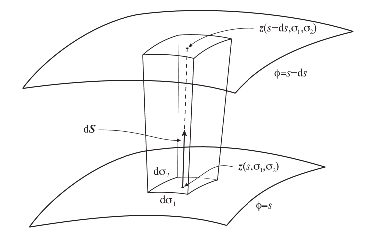
Figure 16: An infinitesimal flux tube. The area element ${\rm d}\bm{S}$ defined in (A.4) is proportional to both $\bm{\nabla}\phi$ and $\frac{\partial\bm{z}}{\partial s}$.

One can also derive the continuum Nahm equation from the Laplace equation. Starting from $\phi(\bm{z})$ satisfying the Laplace equation, we construct $\bm{z}(s,\sigma^{1},\sigma^{2})$ by solving $\phi(\bm{z})=s$. This requires fixing the $\sigma^{1},\sigma^{2}$ coordinates. We first fix $\sigma^{1},\sigma^{2}$ for a given $s$ by the requirement that the flux density be constant as in (A.7). The definition of $\sigma^{1},\sigma^{2}$ can be extended for arbitrary $s$, by requiring that $\frac{\partial\bm{z}}{\partial s}$ be proportional to $\bm{\nabla}\phi$. Once the paramterisation is fixed, one can deduce the continuum Nahm equations from the Laplace equation by basically backtracking the above proof.

Appendix B Behaviour at the splitting point

In this appendix, we discuss the behaviour of families of equipotential surfaces for solutions of the Laplace equation of the type presented in section 4 near points where the splitting occurs.

The splitting point is a singularity of the continuum Nahm equation, which is a partial differential equation (PDE). It is a well-known idea to study such singularities by describing the solutions of a PDE as a level set of a given function [53]. The singular point of the PDE is not singular for the function and thus this approach provides a way to discuss the phenomena described by the PDE avoiding the singularity. In the present case the PDE describes the evolution of a surface and another representation of the same membrane evolution, also free of singularities, is provided by the matrix regularisation. The equivalence between these two regularisations – the level set description of the PDE and the matrix model formulation – is implicitly assumed in our analysis.

In a region sufficiently close to a generic splitting point, the potential $\phi$ can be approximated by 

$$s=\phi(x,y,z)=\frac{1}{2}(x^{2}+y^{2})-z^{2},$$ (B.1)

which satisfies the Laplace equation, up to suitable rescaling of the $x,y,z$ variables. The surface described by (B.1) is a connected hyperboloid, a cone or a disconnected hyperboloid, depending on whether $s>0$, $s=0$ or $s<0$ respectively. The $s=0$ surface embedded in the $(x,y,z)$ space is a cone with tip at $z=0$. The continuum Nahm equations are

$$\dot{x}=-\alpha\{y,z\},\ \ \ \dot{y}=-\alpha\{z,x\},\ \ \ \dot{z}=-\alpha\{x,y\},$$ (B.2)

where $\alpha>0$ and the Lie bracket is defined in (3.4). At the tip of the cone the equations become singular, while the potential (B.1) itself is, of course, non-singular.

The form of the potential (B.1) can be used to study universal features of the splitting point. In particular, in order to discuss the relation between the matrix regularisation and the regularisation via the Laplace equation, one can assume the matrix size to be sufficiently large. Hence one can focus on the vicinity of the splitting point, i.e. the tip of the cone, and the generic form of the potential (B.1) is sufficient.

We discuss the relation of the two regularisations in the following way. Firstly, we rewrite the solution to the Laplace equation near the singularity (B.1) using a hodograph transformation, i.e. exchanging the role of independent and dependent variables, to obtain $x(s,\sigma^{1},\sigma^{2})$, $y(s,\sigma^{1},\sigma^{2})$ and $z(s,\sigma^{1},\sigma^{2})$. As functions of the $(s,\sigma^{1},\sigma^{2})$ these satisfy the continuum Nahm equation (B.2), see [20, 21] and appendix A. It turns out that this solution is characterised by a cubic equation. Then we discretise the functions, $x(\sigma^{1},\sigma^{2})$, $y(\sigma^{1},\sigma^{2})$ and $z(\sigma^{1},\sigma^{2})$, using the matrix regularisation and check if these satisfy the Nahm equations when the matrix size is large enough.

To construct $x$, $y$ and $z$ satisfying (B.1) as functions of $(\sigma^{1},\sigma^{2})$ we proceed as follows. For convenience we introduce a radial coordinate $\rho$,

$$\rho=\sqrt{x^{2}+y^{2}}=\sqrt{2}\sqrt{z^{2}+s}\,,$$ (B.3)

where in the last equality we have used (B.1). We fix the $\sigma$ coordinates by using (A.7). We compute the infinitesimal area in $\sigma$-space as follows. Using

$$\text{d}(\mbox{Area in $(x,y,z)$-space})=2\pi\rho\sqrt{1+\left(\frac{\text{d}\rho}{\text{d}z}\right)^{2}}\text{d}z=2\pi\sqrt{2}\sqrt{3z^{2}+s}\ \text{d}z$$ (B.4)

and

$$\left|\bm{\nabla}\phi\right|=|(x,y,-2z)|=\sqrt{x^{2}+y^{2}+4z^{2}}=\sqrt{6z^{2}+2s}=\sqrt{2}\sqrt{3z^{2}+s},$$ (B.5)

we obtain

$$\text{d}(\mbox{Area in $\sigma$-space})=\alpha 4\pi(3z^{2}+s)\text{d}z.$$ (B.6)

The infinitesimal area above refers to the portion of the membrane between $z$ and $z+\text{d}z$.

We parametrise the $\sigma$-space by $\xi$ and $\varphi$ with range $(-\infty,\infty)$ and $[0,2\pi)$ respectively. We have chosen the parametrisation such that $\xi$ increases as $z$ does and $\varphi$ is the standard polar angle.

Integrating both sides of (B.6) we get a cubic equation,

$$\alpha(z^{3}+sz)=\frac{\xi}{2}\,,$$ (B.7)

from which we obtain $z$ (and $\rho$ via (B.3)) as a function of $\xi$ and $s$. When there exist three solutions in (B.7), we choose a branch: for positive (negative) $\xi$, a positive (negative) root of the equation is employed. For $s>0$ there is only one root for every $\xi\in(-\infty,\infty)$. For $s<0$ there is a discontinuity at $\xi=0$, such that $z=\sqrt{-s}$ and $z=-\sqrt{-s}$ for $\xi\to 0$ from above and $\xi\to 0$ from below, respectively. Therefore, the $\sigma$-space is cylindrical for $s>0$ (corresponding to a connected hyperboloid), whereas it consists of two infinite planes for $s<0$ (corresponding to a disconnected hyperboloid) and a cone for $s=0$. It is interesting that a family of hyperboloids (described for each $s$ by a quadratic equation) is parametrised in this way by a cubic equation.

The $\xi,\varphi$ coordinates thus defined can be identified as the $(\sigma^{1},\sigma^{2})$ coordinates directly so that we have

$$\{f,g\}=\frac{\partial f}{\partial\xi}\frac{\partial g}{\partial\varphi}-\frac{\partial g}{\partial\xi}\frac{\partial f}{\partial\varphi}$$ (B.8)

and

$$\int\text{d}\sigma^{1}\text{d}\sigma^{2}=\int\text{d}\xi\text{d}\varphi.$$ (B.9)

One can study the singularity at the splitting point, using the coordinates $\xi,\varphi$. A natural measure for the singularity is the “energy density”

$$\varepsilon=\frac{1}{2}\left(\{x,y\}^{2}+\{y,z\}^{2}+\{z,x\}^{2}\right).$$ (B.10)

We use the relation between the continuum Nahm equation and the Laplace equation to obtain

$$\varepsilon=\frac{1}{\alpha^{2}|\bm{\nabla}\phi|^{2}}=\frac{1}{\alpha^{2}\left(x^{2}+y^{2}+4z^{2}\right)}=\frac{1}{\alpha^{2}\left(6z^{2}+s\right)}.$$ (B.11)

Thus the “energy density” diverges when $s=0$ at $z=0$ (i.e. $\xi=0$) as

$$\varepsilon\sim\frac{1}{z^{2}}\sim\xi^{-2/3}\,.$$ (B.12)

We note however that the divergence is weak enough so that the integral of the “energy density”

$$\int\varepsilon\text{d}\xi\text{d}\varphi$$ (B.13)

is finite.

The coordinates, $x$, $y$ and $z$, are functions of $(s,\xi,\varphi)$; from (B.7) $z(s,\xi,\varphi)=z(s,\xi)$. The variables $x$ and $y$ can be conveniently described by using

$$w=x+iy=\rho e^{i\varphi},\ \ \ w^{\dagger}=x-iy=\rho e^{-i\varphi}.$$ (B.14)

It is easy to check that the functions $z$ and $w$ satisfy the continuum Nahm equations (B.2),

$$\dot{z}=-\frac{i}{2}\alpha\{w,w^{\dagger}\},\ \ \ \dot{w}=i\alpha\{w,z\},$$ (B.15)

where we have introduced $\dot{z}=\partial_{s}z$ and $z^{\prime}=\partial_{\xi}z$. The above equations are equivalent to

$$\dot{z}=-\alpha\rho^{\prime}\rho,\ \ \ \dot{\rho}=\alpha\rho z^{\prime}.$$ (B.16)

Acting with $\partial_{s}$ and $\partial_{\xi}$ on both sides of the cubic equation (B.7) we have

$$\dot{z}=-\frac{z}{3z^{2}+s},\ \ \ z^{\prime}=\frac{1}{2\alpha(3z^{2}+s)}.$$ (B.17)

Using (B.3), these imply

$$\dot{\rho}=\frac{\sqrt{z^{2}+s}}{\sqrt{2}(3z^{2}+s)},\ \ \ \rho^{\prime}=\frac{z}{\sqrt{2}\alpha\sqrt{z^{2}+s}(3z^{2}+s)}.$$ (B.18)

Substituting into the continuum Nahm equations (B.16) we see that the equations are satisfied.

We then discretise the functions, $z$ and $w$, via the matrix regularisation and we check if they satisfy the Nahm equations when the matrix size is large enough. Here we write the Nahm equations in the form

$$\dot{X}=-\alpha\frac{1}{iC}[Y,Z]\ \ \ \dot{Y}=-\alpha\frac{1}{iC}[Z,X],\ \ \ \dot{Z}=-\alpha\frac{1}{iC}[X,Y],$$ (B.19)

or equivalently,

$$\dot{Z}=-\frac{\alpha}{2C}[W,W^{\dagger}],\ \ \ \dot{W}=\frac{\alpha}{C}[W,Z],$$ (B.20)

where

$$W=X+iY,\ \ \ W^{\dagger}=X-iY.$$ (B.21)

Here $X$, $Y$, $Z$ and $W$ are infinite dimensional matrices (corresponding to the non-compact $\sigma$-space). If the original matrix size $J$ is sufficiently large, we have $C\ll 1$. 

Our ansatz for the matrices is as follows [27, 54]. We take $Z$ to be diagonal and assume that $W$ has only non-zero sub-diagonal entries, i.e. the only non-zero components in the matrices are $Z_{mm}=Z_{m}$, $W_{m,m+1}$ respectively. We use a slightly unusual convention in which the rows and columns of infinite-size matrices are labelled by half-integer valued indices. The index $m$ can take both positive values, $m=1/2,3/2,5/2,\ldots$, and negative values, $m=-1/2,-3/2,-5/2,\ldots$ Using this ansatz, we propose a candidate for an approximate solution to the Nahm equations (B.20). For this purpose, we introduce an auxiliary function, $z[m]$, defined as a root of the cubic equation

$$z^{3}+sz=\frac{C}{2\alpha}m.$$ (B.22)

In case this equation has three solutions, we choose a branch in the same way as described below (B.7). Note that in (B.22) we have discretised $\xi$ introduced in (B.7) as $\xi=Cm$, i.e. the mesh of $\xi$ is taken to be equally spaced, following the Bohr-Sommerfeld quantisation [27]. Then the approximate solution to the Nahm equations (B.20) is

$$Z_{mm}=z[m],$$ (B.23)

$$W_{m,m+1}=\sqrt{2}\sqrt{z[m+1/2]^{2}+s}\,.$$ (B.24)

Note that this equation is well-defined even for $W_{-1/2,+1/2}$ for $s<0$; $z[m]$ has a discontinuity at $m=0$, but $z[m]^{2}$ does not. Furthermore, we note that $W_{-1/2,+1/2}=0$ here. For $s<0$ there are two disconnected portions, i.e. the two sheets of the hyperboloid. The values, $m=-1/2$ and $m=1/2$, correspond to these two parts and we do not expect non-zero matrix elements between them.

We show that these matrices satisfy the Nahm equations (B.20) up to terms which are sub-leading for $C\ll 1$. Indeed,

$$[W,W^{\dagger}]_{mm} =W_{m,m+1}^{2}-W_{m-1,m}^{2}$$

$$\approx 2\left(z\left[m+1/2\right]-z\left[m-1/2\right]\right)\left(z\left[m+1/2\right]+z\left[m-1/2\right]\right)$$

$$\approx 4z[m]\frac{\partial}{\partial m}z[m]\approx-\frac{2C}{\alpha}\dot{Z}_{mm}.$$ (B.25)

Similarly, since

$$[W,Z]_{m,m+1} =\left(z[m+1]-z[m]\right)W_{m,m+1}$$

$$\approx\sqrt{2}\sqrt{z[m]^{2}+s}\ \frac{\partial}{\partial m}z[m]=\frac{C}{\alpha}\frac{\sqrt{z[m]^{2}+s}}{\sqrt{2}(3z[m]^{2}+s)}$$ (B.26)

and

$$\dot{W}_{m,m+1} =\frac{2z\left[m+1/2\right]\dot{z}\left[m-1/2\right]+1}{W_{m,m+1}}\approx\frac{\sqrt{z[m]^{2}+s}}{\sqrt{2}(3z[m]^{2}+s)},$$ (B.27)

we have

$$[W,Z]_{m,m+1}\approx\frac{C}{\alpha}\dot{W}_{m,m+1}.$$ (B.28)

The existence of the approximate solution suggests that there exist an exact solution with the same qualitative behaviour. It would be also interesting to find the exact solution of the Nahm equations within the tridiagonal ansatz made above. In that case, it is known that the Nahm equations are closely related to those describing the so-called Toda lattice.

Appendix C Other solutions

C.1 BHP solution

The BHP solution (2.21) describes an instanton interpolating between a representation $L^{i}_{(-\infty)}$ at $t=-\infty$ and the $J$-dimensional representation ${\underline{1}}\oplus{\underline{1}}\oplus\cdots\oplus{\underline{1}}$ at $t=+\infty$. We consider the special case in which $L^{i}_{(-\infty)}$ is the irreducible representation ${\underline{J}}$. This corresponds to a process in which a membrane with angular momentum $J$ shrinks to a point-like object. Extrapolating the interpretation of the vacuum associated with a direct sum of irreducible representations as a collection of concentric membranes, the final state may be thought of as consisting of $J$ membranes each carrying one unit of angular momentum. However, we stress that such an extrapolation goes well beyond the region of applicability of the approximations used in this paper. Using the proposal in [42], the final state can also be understood as corresponding to a single M5-brane carrying angular momentum $J$.

It is not difficult to construct a solution to the Laplace equation which approximates this instanton configuration. To obtain a solution with the right properties, we consider the Coulomb potential generated by a positive point charge $J$ at the origin with the addition of a negative constant,

$$\phi(\bm{z})=\frac{J}{4\pi|\bm{z}|}-e^{-2t_{0}/R},$$ (C.1)

where $\bm{z}=(z^{1},z^{2},z^{3})$. Using the transformation (3.7) in reverse order, one can compute the distance from the origin of the membrane corresponding to (C.1) in terms of the variables $\bm{y}=(y^{1},y^{2},y^{3})$. The result is

$$|\bm{y}(t)|=\frac{J}{(2\pi T)R^{2}}\frac{1}{1+e^{2(t-t_{0})/R}}\,.$$ (C.2)

This represents a sphere with time dependent radius, $r(t)=|\bm{y}(t)|$, given by the right hand side of (C.2). For large values of the potential, i.e. $|\bm{z}|\approx 0$, corresponding to the far past ($t\to-\infty$), (C.1)-(C.2) describe a configuration which approaches a stable sphere of radius $r=J/(2\pi TR^{2})$. On the other hand, the potential (C.1) becomes zero at a finite distance from the origin, $|\bm{z}|=J/(4\pi e^{-2t_{0}/R})$, in the far future ($t\to+\infty$), where the radius of the membrane, $|\bm{y}|$, shrinks to zero.

The explicit form of the continuum counterpart of the BHP solution, in the case in which $L^{i}_{(-\infty)}$ is irreducible, is therefore

$$y^{i}(t,\sigma^{1},\sigma^{2})=r(t)n^{i}(\sigma^{1},\sigma^{2}),$$ (C.3)

where the membrane radius is

$$r(t)=\frac{J}{(2\pi T)R^{2}}\frac{1}{1+e^{2(t-t_{0})/R}}$$ (C.4)

and $n^{i}(\sigma^{1},\sigma^{2})$ is a unit vector in the radial direction.

C.2 Solution with positive and negative point charges

In this section we present a new solution approximately describing the instanton interpolating between the irreducible vacuum ${\underline{J}}$ and the vacuum associated with the representation ${\underline{J}}^{\prime}\oplus{\underline{1}}\oplus\cdots\oplus{\underline{1}}$, where ${\underline{1}}$ appears with multiplicity $(J-J^{\prime})$. From the membrane point of view in this process a single membrane with angular momentum $J$ splits into a membrane with angular momentum $J^{\prime}$ and a second membrane which shrinks to a point in the final state.

The corresponding solution to the Laplace equation is the sum of two Coulomb potentials associated respectively with a positive charge $J$ at the origin and a negative charge of magnitude $(J-J^{\prime})$ at a point $\bm{z}=\bm{z}_{0}(\neq\bm{0})$,

$$\phi(\bm{z})=\frac{J}{4\pi|\bm{z}|}-\frac{J-J^{\prime}}{4\pi|\bm{z}-\bm{z}_{0}|}\,,$$ (C.5)

where $J^{\prime}$ is assumed to be positive. The evolution of the membrane profile, corresponding to the equipotential surfaces of (C.5), can be described as follows. The relevant equipotential surfaces are those with $s=\phi\in(+\infty,0]$ which corresponds to $t\in(-\infty,+\infty)$. For $t\sim-\infty$, i.e. $s=\phi\sim+\infty$, we have a single spherical membrane of small radius. As $t$ increases this membrane grows and deforms, until it splits into two membranes (both with spherical topology) at a value $s>0$ of the potential. One of the membranes continues to grow as $t$ increases towards $+\infty$, i.e. $s=\phi\to 0$, and approaches the behaviour of the equipotential surfaces of a Coulomb solution with charge $J^{\prime}$. The other membrane at $\phi\sim 0$ is a sphere of finite radius. (This is a well-known fact used for the electrostatic potential of a spherical conductor.) The first membrane, due to the transformation (3.7), corresponds to a static spherical membrane in the original $\bm{y}$ coordinates (see section 4.1). In the same coordinates the second membrane shrinks to a point. Therefore, one finds indeed that the potential (C.5) describes the process in which a spherical membrane with angular momentum $J$ at $t=-\infty$ splits into a spherical membrane with angular momentum $J^{\prime}$ and a point-like object carrying angular momentum $(J-J^{\prime})$ .

A description of the above solution in terms of a suitable Riemann space leads to an interesting interpretation for the negative point charge. We consider a Riemann space consisting of $m+1$ sheets, with $m$ identical branch disks connecting the first sheet to the remaining $m$ sheets. The insertion of the negative charge can be realised as the limit in which $m$ is sent to infinity while the size of the branch disks is sent to zero, so as to keep the total flux out of the first sheet fixed.

It is clear that this solution can be generalised. One can put an arbitrary number of negative point charges at arbitrary locations. It is also possible to put the negative charges on different sheets of a Riemann space.

As mentioned earlier the ${\underline{1}}\oplus\cdots\oplus{\underline{1}}$ solution was conjectured in [42] to represent a single M5-brane. It is interesting to notice that combining this proposal with the above considerations, we are led to the conclusion that while M2-branes in our construction correspond to positive charges (which should be located at the origin of each sheet of a Riemann space), negative charges (which can be placed at arbitrary locations) are associated with M5-branes.

Appendix D Relation between Hobson’s and Sommerfeld’s solutions

The solution found by Sommerfeld [23] is

$$\phi(\bm{r},\bm{r_{0}})=\frac{1}{|\bm{r}-\bm{r_{0}}|}\left(\frac{1}{2}+\frac{1}{\pi}\arcsin{\left(\frac{\cos{\frac{\varphi_{S}-\varphi_{S0}}{2}}}{\cosh{\frac{\alpha_{S}}{2}}}\right)}\right),$$ (D.1)

where

$$\cosh\alpha_{S}=\frac{r_{S}^{2}+r_{S0}^{2}+(z_{S}-z_{S0})^{2}}{2r_{S}r_{S0}},$$ (D.2)

up to an overall constant. The notation used in the above formulae is as follows. We use the standard cylindrical coordinates $(r_{S},\varphi_{S},z_{S})$ for the point $\bm{r}$ where the $z$-axis coincides with the straight branch line. For the source point $\bm{r_{0}}$ the cylindrical coordinates are $(r_{S0},\varphi_{S0},z_{S0})$.

The solution is related to Hobson’s solution by an inversion tranformation, where the point of inversion $A$ is taken to be a point on the circumference of the disk. It is clear that the circular branch loop in Hobson’s solution is mapped to the straight branch line in Sommerfeld’s solution. The relation between the two solutions was observed and numerically verified in work by Heise [30]. Below we provide an analytic proof.

For the purpose of comparison, we present here again Hobson’s solution (4.13), (4.14) in an appropriately normalised form,

$$\phi(\bm{r},\bm{r}_{0})=\frac{1}{|\bm{r}-\bm{r}_{0}|}\left(\frac{1}{2}+\frac{1}{\pi}\arcsin\!\left(\frac{\cos\frac{\theta_{H}-\theta_{H0}}{2}}{\cosh\frac{\alpha_{H}}{2}}\right)\right)\,,$$ (D.3)

where

$$\cosh\alpha_{H}=\cosh\rho_{H}\cosh\rho_{H0}-\cos(\varphi_{H}-\varphi_{H0})\sinh\rho_{H}\sinh\rho_{H0}$$ (D.4)

and $(\rho_{H},\theta_{H},\varphi_{H})$ are the peripolar coordinates defined in section 4.2.2. We note that we have used

$$\cosh{\frac{\alpha_{H}}{2}}=\sqrt{\frac{\cosh\alpha_{H}+1}{2}}.$$ (D.5)

In this appendix we use the subscripts $H$ and $S$ to emphasise the distinction between the coordinates and the variables used in Hobson’s and Sommerfeld’s solutions.

In order to show that the solution (D.3) maps to (D.1) under an inversion transformation, we note that the prefactor $1/|\bm{r}-\bm{r}_{0}|$ in both solutions transforms under an inversion transformation in the well-known manner. Hence to show the equivalence between (D.3) and (D.1) under the inversion transformation it is sufficient to prove the following identities

$$\varphi_{S}=\theta_{H},$$ (D.6)

$$\alpha_{S}=\alpha_{H}.$$ (D.7)

The first identity needs only be satisfied up to a sign and constant shifts because the variables in the formula always appear in combinations such as $\cos{((\varphi_{S}-\varphi_{S0})/2)}$.

To prove (D.6) we first focus on the plane which contains the point of inversion $A$ and the center of the branch disk and which is orthogonal to the branch disk. The definition of $\theta_{H}$ is depicted in the first panel of figure 3. We denote by $P^{\prime},B^{\prime}$ the points corresponding to $P,B$ by an inversion transformation around the point $A$. By definition we have $\widehat{APB}=\theta_{H}$. We also have $\widehat{P^{\prime}B^{\prime}A}=\varphi_{S}$, since the straight branch line passes through the plane orthogonally at the point $B^{\prime}$. By elementary geometry, it is easy to show that $\widehat{APB}=\widehat{P^{\prime}B^{\prime}A}$, which is (D.6), using the definition of the inversion transformation. It is possible furthermore to show that the validity of (D.6) can be extended to the whole $\mathbbm{R}^{3}$. Indeed, we observe that the constant $\theta_{H}$ surface in Hobson’s coordinate is a part of a sphere bounded by the branch loop. Since the surface contains the inversion point, it will be mapped to a half-plane bounded by the straight branch line. Thus a constant $\theta_{H}$ surface is mapped to a constant $\varphi_{S}$ surface under the inversion and therefore it follows that (D.6) is valid generally.

It finally remains to show (D.7). As $\alpha_{H}$ and $\alpha_{S}$ do not depend on the $\theta_{H}=\varphi_{S}$ variable, one can focus on the special case $\theta_{H}=\pi$. The quantity $\alpha_{H}$ will then be defined on a pair of points on the branch disk itself and we wish to show that it is equal to $\alpha_{S}$ for the corresponding pair of points on the branch half-plane. This can be established by noting that $\alpha_{S}$ and $\alpha_{H}$ are nothing but the geodesic distances in the classic Poincaré upper half plane and disk models (the latter also referred to as the conformal disk model) of hyperbolic geometry, respectively [55]. These two models are related to each other by an inversion transformation and hence (D.7) follows.

It is interesting to note that the quantity $\alpha_{H}$ (or $\alpha_{S}$), which is an important ingredient in the exact solution, has an interpretation in terms of some non-trivial geometry defined on the branch disk (or the branch half-plane).

Appendix E Boundary conditions at branch disks and reformulation in terms of integral equations

In this appendix, we formulate boundary conditions associated with branch disks and present a reformulation of the Laplace equation on a Riemann space in terms of a set of integral equations. The unknown variables in the integral equations are functions defined on the branch surfaces. Here we use the vector $\bm{r}=(x,y,z)$ to denote the position of a point in what was referred to as $z$-space in the main text.

For concreteness we focus on the simplest case where there are two copies of $\mathbbm{R}^{3}$ connected by a single branch disk $D$. We put a point charge $J$ at the point designated by a vector $\bm{r_{0}}$. The potential function will be denoted by $\phi_{(1)}(\bm{r})$ in the first space and by $\phi_{(2)}(\bm{r})$ in the second space.

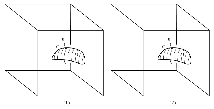
Figure 17: Riemann spaces

As functions in $\mathbbm{R}^{3}$ both these potential functions have a discontinuity at the branch disk. In order to take care of this discontinuity, we introduce the following notation. We refer to the two sides of the branch disk as $a$ and $b$. The values of the potential functions in each space, $\phi_{(i)}$, $(i=1,2)$, on the $a$ and $b$ sides of the branch disk will be denoted respectively by

$$\phi_{(i)a}(\bm{r})\quad{\rm and}\quad\phi_{(i)b}(\bm{r}).$$ (E.1)

In these expressions it is implicitly assumed that the vector $\bm{r}$ corresponds to a point on the branch disk which is approached from the $a$ or $b$ side.

We introduce the normal vector orthogonal to the branch disk defined at the point on the branch disk, $\bm{n}$, with orientation such that $\bm{n}$ points away from the disk on the $a$ side and towards the disk on the $b$ side as shown in figure 17.

The precise formulation of the condition that the first and the second spaces are connected by the branch disk is given by the following formulae,

$$\phi_{(1)a}(\bm{r})=\phi_{(2)b}(\bm{r}),\qquad\phi_{(2)a}(\bm{r})=\phi_{(1)b}(\bm{r}),$$ (E.2)

and

$$\partial_{n}\phi_{(1)a}(\bm{r})=\partial_{n}\phi_{(2)b}(\bm{r}),\qquad\partial_{n}\phi_{(2)a}(\bm{r})=\partial_{n}\phi_{(1)b}(\bm{r}),$$ (E.3)

where $\partial_{n}\phi(\bm{r})$ denotes the normal derivative of the potential functions at the branch disk,

$$\partial_{n}\phi(\bm{r})=\bm{n}\cdot\bm{\nabla}\phi.$$ (E.4)

We further require, as a part of the boundary conditions, that the $\phi_{(i)}$’s be finite at the boundary of the branch disk (the branch loop) and that they go to zero at infinity sufficiently rapidly.

Below we reformulate the Laplace equations with given boundary conditions in terms of integral equations. This reformulation is known, in the case of more conventional boundary conditions, to be useful in many respects, including numerical computations and the study of existence and uniqueness properties for the solutions to the Laplace equation [56]. We will use Green’s theorem,

$$\int_{M}\left(\phi\bm{\nabla}^{2}\psi-\psi\bm{\nabla}^{2}\phi\right)(\bm{r^{\prime}})\text{d}^{3}\bm{r^{\prime}}=\int_{\partial M}\left(\phi\bm{\nabla}\psi-\psi\bm{\nabla}\phi\right)(\bm{r^{\prime}})\cdot\text{d}^{2}\bm{S^{\prime}},$$ (E.5)

for the special case where $\psi(\bm{r^{\prime}})$ is

$$\psi(\bm{r^{\prime}})=-\frac{1}{4\pi|\bm{r}^{\prime}-\bm{r}|}\,,$$ (E.6)

satisfying

$$\bm{\nabla}^{2}\psi(\bm{r^{\prime}})=\delta^{3}(\bm{r}^{\prime}-\bm{r}).$$ (E.7)

The potential on the first sheet, $\phi_{(1)}$, also has a $\delta$-function source,

$$-\bm{\nabla}^{2}\phi_{(1)}(\bm{r}^{\prime})=J\delta^{3}(\bm{r}^{\prime}-\bm{r_{0}})$$ (E.8)

or equivalently behaves as

$$\phi_{(1)}(\bm{r^{\prime}})\sim\frac{J}{4\pi|\bm{r}^{\prime}-\bm{r_{0}}|},$$ (E.9)

when $|\bm{r}^{\prime}-\bm{r_{0}}|\sim 0$.

We define the following two important functions on the branch disk,

$$f=\phi_{(1)a}-\phi_{(1)b},$$ (E.10)

$$g=\partial_{n}\phi_{(1)a}-\partial_{n}\phi_{(1)b}.$$ (E.11)

They are the discontinuities of the potential and the normal derivative (in the first space).

The functions $f$ and $g$ may be interpreted as the dipole moment density and the charge density of a fictitious charge distribution placed at the disk, which, together with the point charge at $\bm{r}_{0}$, reproduces the electrostatic potential $\phi_{(1)}$. The functions $f$ and $g$ are the two unknown functions in the reformulation in terms of integral equations.

We apply Green’s theorems to $\phi_{(i)}$, choosing for $M$ the region in $\mathbbm{R}^{3}$ obtained excluding the branch disk . We then obtain

$$\phi_{(1)}(\bm{r})=\frac{J}{4\pi|\bm{r}-\bm{r_{0}}|}+\chi(\bm{r}),$$ (E.12)

$$\phi_{(2)}(\bm{r})=-\chi(\bm{r}).$$ (E.13)

Here we have introduced $\chi(\bm{r})$ defined as

$$\chi(\bm{r})=\int_{D}\left(-f(\bm{r}^{\prime})\frac{1}{4\pi}\frac{(\bm{r}^{\prime}-\bm{r})}{|\bm{r}^{\prime}-\bm{r}|^{3}}\cdot\bm{n}-g(\bm{r}^{\prime})\frac{1}{4\pi}\frac{1}{|\bm{r}-\bm{r}^{\prime}|}\right)\text{d}^{2}S^{\prime},$$ (E.14)

where the integration variable, $\bm{r}^{\prime}$, is restricted to the branch disk. Here, the condition that the $\phi_{(i)}$’s themselves be finite at the branch loop is important. Without this condition, it is possible to have an extra term in the above formulae originating from the branch loop. (Consider superposing to the $\phi_{(i)}$’s the electrostatic potential generated by a charged wire placed at the branch loop.)

Formulae (E.12)-(E.14) give an integral representation of the potential on the two sheets of the Riemann space, in terms of the discontinuities $f$ and $g$ at the branch disk.

Substituting the integral representations back into the connecting conditions (E.2)-(E.3), one obtains

$$\chi_{a}(\bm{r})+\chi_{b}(\bm{r})=-\frac{J}{4\pi|\bm{r}-\bm{r}_{0}|},$$ (E.15)

$$\partial_{n}\chi_{a}(\bm{r})+\partial_{n}\chi_{b}(\bm{r})=-\frac{1}{4\pi}\partial_{n}\frac{J}{|\bm{r}-\bm{r}_{0}|}.$$ (E.16)

Here $\bm{r}$ is assumed to correspond to points on the branch disk. The function $\chi$ also has a discontinuity across the disk and we denote by $\chi_{a}$ and $\chi_{b}$ the values of $\chi$ on side $a$ and $b$ respectively. Formulae (E.14)-(E.16) are the integral equations for the functions $f$ and $g$, which are defined on the disk.

Focussing on the special case in which the disk $D$ lies in the $xy$-plane, one can rewrite the integral equations in a more explicit form as

$$\int_{D}\frac{1}{\sqrt{(x-x^{\prime})^{2}+(y-y^{\prime})^{2}}}g(x^{\prime},y^{\prime})\text{d}x^{\prime}\text{d}y^{\prime}$$

$$\ \ \ =\frac{1}{2}\frac{J}{|\bm{r}-\bm{r}_{0}|}=\frac{1}{2}\frac{J}{\sqrt{(x-x_{0})^{2}+(y-y_{0})^{2}+z_{0}^{2}}},$$ (E.17)

$$\int_{D}\left(\frac{-1}{\sqrt{(x-x^{\prime})^{2}+(y-y^{\prime})^{2}+\varepsilon^{2}}^{3}}+\frac{3\varepsilon^{2}}{\sqrt{((x-x^{\prime})^{2}+(y-y^{\prime})^{2}+\varepsilon^{2}}^{5}}\right)f(x^{\prime},y^{\prime})\text{d}x^{\prime}\text{d}y^{\prime}$$

$$\ \ \ =\frac{1}{2}\partial_{z}\frac{J}{|\bm{r}-\bm{r}_{0}|}=J\frac{z_{0}}{\sqrt{(x-x_{0})^{2}+(y-y_{0})^{2}+z_{0}^{2}}^{3}}.$$ (E.18)

They are Fredholm integral equations of the first type, the second integral equation having a singular kernel. We note that the first integral equation is equivalent to the integral equation for the electrostatic potential associated with a conducting disk.

Appendix F Equations for general pp-wave matrix model

In the main text we have given most of the formulae for the pp-wave matrix model which is relevant for the large $J$ sector of the ABJM duality in the special case $k=1$. In this appendix we give generalisations of some of the important equations to the general pp-wave matrix model written in terms of a mass parameter, $\mu$, and for $k\neq 1$. To make the use of the generalised formulae below more straightforward we have numbered each equation with the same equation number as the corresponding one in the main text, with the addition of a suffix “a”. So for example equation (2.1a) below is the generalisation of (2.1) in section 2.

Below we consider matrices of size

$$K=\frac{J}{k}.$$ (F.1)

We note that the angular momentum quantum number $J$ is a multiple of $k$ on $S^{7}/\mathbbm{Z}_{k}$. The radius of $S^{7}$, $R$, is related to the radius of the M-theory circle, $R_{11}$, by

$$R_{11}=\frac{R}{k}.$$ (F.2)

For the pp-wave approximation of AdS${}_{4}\times S^{7}/\mathbbm{Z}_{k}$, the mass parameter $\mu$ below should be set to the value,

$$\mu=\frac{6}{R}.$$ (F.3)

All formulae in the rest of this appendix are written in terms of the parameters $K$, $R_{11}$ and $\mu$. In order to generalise the formulae in the main text to the $k\neq 1$ case, it is sufficient to apply (F.2) and (F.3) to the equations below and remember that the matrix size $K$ is given by (F.1).

Using the replacements $X^{m}\to-X^{m}$ and $Y^{i}\to-Y^{i}$, changing the sign of the mass parameter, $\mu\to-\mu$, and setting $2\pi T=1$ brings the following equations to the form used in the literature on the pp-wave matrix model, e.g. [6]. Note that the redefinition of $\mu$ and $Y$ has the effect of exchanging instantons and anti-instantons, which can be seen from (2.12a).

$$S_{E}=\int {\rm d}t\;\text{tr}\biggl{\{}\frac{1}{2R_{11}}\left(\frac{DY^{i}}{Dt}\right)^{2}+\frac{1}{2R_{11}}\left(\frac{DX^{m}}{Dt}\right)^{2}$$

$$+(2\pi T)^{2}\frac{R_{11}}{4}\left((i[X^{m},X^{n}])^{2}+2(i[X^{m},Y^{i}])^{2}\right)$$

$$+\frac{1}{2R_{11}}\left(\frac{\mu}{6}\right)^{2}(X^{m})^{2}+(2\pi T)^{2}\frac{R_{11}}{2}\left(\frac{i}{2}\epsilon^{ijk}[Y^{j},Y^{k}]+\frac{\mu}{3(2\pi T)R_{11}}Y^{i}\right)^{\!\!2}$$

$$+\frac{1}{2}\Psi^{T}\frac{D\Psi}{Dt}+2\pi T\frac{R_{11}}{2}\left(\Psi^{T}\gamma^{m}[X^{m},\Psi]+\Psi^{T}\gamma^{i}[Y^{i},\Psi]\right)-i\frac{\mu}{8}\,\Psi^{T}\gamma^{123}\Psi\biggl{\}}.$$ (2.1a)

$$Y_{0}^{i}=\frac{\mu}{3(2\pi T)R_{11}}L^{i}\,,\quad{\rm with}\quad[L^{i},L^{j}]=i\epsilon^{ijk}L^{k}\,.$$ (2.3a)

$$r=\frac{\mu\sqrt{K^{2}-1}}{6(2\pi T)R_{11}}\approx\frac{\mu K}{6(2\pi T)R_{11}}\,.$$ (2.5a)

$$S_{E}=\frac{1}{2R_{11}}\int{\rm d}t\>\text{tr} \biggl{[}\left(\frac{\text{d}X^{m}}{\text{d}t}\right)^{2}+\left(\frac{\mu}{6}\right)^{2}\left(X^{m}\right)^{2}+\frac{(2\pi T)^{2}R^{2}_{11}}{2}\left\{(i[X^{m},X^{n}])^{2}+(i[X^{m},Y^{i}])^{2}\right\}$$

$$+\left(\frac{\text{d}Y^{i}}{\text{d}t}\pm\frac{\mu}{3}Y^{i}\pm i(2\pi T)\frac{R_{11}}{2}\epsilon^{ijk}[Y^{j},Y^{k}]\right)^{2}$$

$$\mp\frac{\text{d}}{\text{d}t}\left(\frac{\mu}{3}Y^{i}Y^{i}+i(2\pi T)\frac{R_{11}}{3}\epsilon^{ijk}Y^{i}[Y^{j},Y^{k}]\right)+{\rm fermions}\biggl{]}\,.$$ (2.8a)

$$S_{E}\geq\left.\mp\frac{1}{2R_{11}}\,W[Y]\right|_{-\infty}^{+\infty}=\mp\frac{\mu}{18R_{11}}\left(\frac{\mu}{3(2\pi T)R_{11}}\right)^{\!2}{\rm tr}\!\left(L^{i}_{(+\infty)}L^{i}_{(+\infty)}-L^{i}_{(-\infty)}L^{i}_{(-\infty)}\right)\,.$$ (2.10a)

$$W[Y]={\rm tr}\left(\frac{\mu}{3}Y^{i}Y^{i}+i(2\pi T)\frac{R_{11}}{3}\epsilon^{ijk}Y^{i}[Y^{j},Y^{k}]\right)\,.$$ (2.11a)

$$\frac{\text{d}Y^{i}}{\text{d}t}\pm\frac{\mu}{3}Y^{i}\pm i(2\pi T)\frac{R_{11}}{2}\epsilon^{ijk}[Y^{j},Y^{k}]=0\,.$$ (2.12a)

$$W[Y_{0}]=\frac{\mu}{9}\left(\frac{\mu}{3(2\pi T)R_{11}}\right)^{\!2}{\rm tr}\!\left(L^{i}L^{i}\right)=\frac{\mu}{9}\left(\frac{\mu}{3(2\pi T)R_{11}}\right)^{2}\frac{1}{4}\sum^{n}_{i=1}{\rm tr}\left[\left(K^{2}_{i}-1\right)\mathbbm{1}_{K_{i}\times K_{i}}\right]\,,$$ (2.15a)

where $K_{j}=J_{j}/k$, $j=1,2,\ldots,n$, denote the (integer) size of the blocks in the case in which the matrices $L^{i}$ are generators of a reducible SU(2) representation. The $K_{j}$’s satisfy $\sum_{j}K_{j}=K$.

$$Z^{i}=C\,e^{(\mu t)/3}Y^{i},\ \ \ s=e^{-(\mu t)/3}\,.$$ (2.18a)

$$\frac{\text{d}Z^{i}}{\text{d}s}=i(2\pi T)\frac{3R_{11}}{2C\mu}\epsilon^{ijk}[Z^{j},Z^{k}]\,.$$ (2.19a)

$$\rho(fg) \approx\frac{1}{2}\Big{(}\rho(f)\rho(g)+\rho(g)\rho(f)\Big{)}\,.$$ (3.1a)

$$\rho\left(\{f,g\}\right) \approx\frac{2\pi K}{i[\sigma]}\left[\rho(f),\rho(g)\right]\,.$$ (3.2a)

$$\frac{1}{[\sigma]}\int f\,{\rm d}^{2}\sigma \approx\frac{1}{K}{\rm tr}\big{(}\rho(f)\big{)}\,.$$ (3.3a)

$$\frac{\partial y^{i}}{\partial t}\pm\frac{\mu}{3}y^{i}\mp\frac{(2\pi T)R_{11}}{4\pi}\frac{[\sigma]}{K}\epsilon^{ijk}\{y^{j},y^{k}\}=0\,.$$ (3.6a)

$$z^{i}=\frac{(2\pi T)}{4\pi}\left(\frac{6}{\mu}\right)^{2}e^{(\mu t)/3}y^{i},\ \ \ s=e^{-(\mu t)/3}\,.$$ (3.7a)

$$\frac{\partial z^{i}}{\partial s}=-\frac{\mu R_{11}}{12}\frac{[\sigma]}{K}\epsilon^{ijk}\{z^{j},z^{k}\}\,.$$ (3.8a)

References

- [1] B. de Wit, J. Hoppe and H. Nicolai, “On the Quantum Mechanics of Supermembranes”, Nucl. Phys. B305 (1988) 545.
- [2] T. Banks, W. Fischler, S. H. Shenker and L. Susskind, “M theory as a matrix model: A Conjecture”, Phys. Rev. D55 (1997) 5112 [hep-th/9610043].
- [3] O. Aharony, O. Bergman, D. L. Jafferis and J. Maldacena, “N=6 superconformal Chern-Simons-matter theories, M2-branes and their gravity duals”, JHEP 0810 (2008) 091 [arXiv:0806.1218 [hep-th]].
- [4] S. Kovacs, Y. Sato and H. Shimada, “Membranes from monopole operators in ABJM theory: Large angular momentum and M-theoretic AdS4/CFT3”, PTEP 2014 (2014) 9, 093B01 [arXiv:1310.0016 [hep-th]].
- [5] D. E. Berenstein, J. M. Maldacena and H. S. Nastase, “Strings in flat space and pp waves from N=4 superYang-Mills”, JHEP 0204 (2002) 013 [hep-th/0202021].
- [6] K. Dasgupta, M. M. Sheikh-Jabbari and M. Van Raamsdonk, “Matrix perturbation theory for M theory on a PP wave”, JHEP 0205 (2002) 056 [hep-th/0205185].
- [7] H. Shimada, “Holography at string field theory level: Conformal three point functions of BMN operators”, Phys. Lett. B647 (2007) 211 [hep-th/0410049].
- [8] S. Dobashi, H. Shimada and T. Yoneya, “Holographic reformulation of string theory on AdS(5) x S**5 background in the PP wave limit”, Nucl. Phys. B665 (2003) 94 [hep-th/0209251].
- [9] S. Dobashi and T. Yoneya, “Resolving the holography in the plane-wave limit of AdS/CFT correspondence”, Nucl. Phys. B711 (2005) 3 [hep-th/0406225].
- [10] S. Dobashi and T. Yoneya, “Impurity non-preserving 3-point correlators of BMN operators from PP- wave holography. I. Bosonic excitations”, Nucl. Phys. B711 (2005) 54 [hep-th/0409058].
- [11] S. Dobashi, “Impurity Non-Preserving 3-Point Correlators of BMN Operators from PP-Wave Holography. II. Fermionic Excitations,” Nucl. Phys. B756 (2006) 171 [hep-th/0604082].
- [12] G. Grignani and A. V. Zayakin, “Matching Three-point Functions of BMN Operators at Weak and Strong coupling”, JHEP 1206 (2012) 142 [arXiv:1204.3096 [hep-th]].
- [13] G. Grignani and A. V. Zayakin, “Three-point functions of BMN operators at weak and strong coupling II. One loop matching”, JHEP 1209 (2012) 087 [arXiv:1205.5279 [hep-th]].
- [14] W. Schulgin and A. V. Zayakin, “Three-BMN Correlation Functions: Integrability vs. String Field Theory One-Loop Mismatch”, JHEP 1310 (2013) 053 [arXiv:1305.3198 [hep-th]].
- [15] B. Basso, S. Komatsu and P. Vieira, “Structure Constants and Integrable Bootstrap in Planar N=4 SYM Theory”, arXiv:1505.06745 [hep-th].
- [16] Y. Kazama, S. Komatsu and T. Nishimura, “On the singlet projector and the monodromy relation for psu(2,24) spin chains and reduction to subsectors”, JHEP 1509 (2015) 183 [arXiv:1506.03203 [hep-th]].
- [17] J. -T. Yee and P. Yi, “Instantons of M(atrix) theory in PP wave background”, JHEP 0302 (2003) 040 [hep-th/0301120].
- [18] C. Bachas, J. Hoppe and B. Pioline, “Nahm equations, N=1* domain walls, and D strings in AdS(5) x S(5)”, JHEP 0107 (2001) 041 [hep-th/0007067].
-
[19]
W. Nahm, “A Simple Formalism for the BPS Monopole”,
Phys. Lett. B90 (1980) 413;
W. Nahm, “All Selfdual Multi - Monopoles For Arbitrary Gauge Groups”, CERN-TH-3172, C81-08-31.1-1. - [20] R. S. Ward, “Linearization of the SU(infinity) Nahm Equations”, Phys. Lett. B234 (1990) 81.
- [21] J. Hoppe, “Surface motions and fluid dynamics”, Phys. Lett. B335 (1994) 41 [hep-th/9405001].
- [22] M. Bordemann and J. Hoppe, “Diffeomorphism invariant integrable field theories and hypersurface motions in Riemannian manifolds”, J. Math. Phys. 39 (1998) 683 [hep-th/9512001].
- [23] A. Sommerfeld, “Über verzweigte Potentiate im Raum”, Proc. London Math. Soc. 28 (1896) 395.
- [24] P. B. Kronheimer, “Instantons and the geometry of the nilpotent variety”, J. Diff. Geom. 32 (1990) 473.
- [25] K. Dasgupta, M. M. Sheikh-Jabbari and M. Van Raamsdonk, “Protected multiplets of M theory on a plane wave”, JHEP 0209 (2002) 021 [hep-th/0207050].
-
[26]
J. Goldstone, unpublished (1982).
J. Hoppe, PhD Thesis (M.I.T. 1982). - [27] H. Shimada, “Membrane topology and matrix regularization”, Nucl. Phys. B685 (2004) 297 [hep-th/0307058].
- [28] E. G. Floratos and G. K. Leontaris, “Integrability of the Selfdual Membranes in (4+1)-dimensions and the Toda Lattice”, Phys. Lett. B223 (1989) 153.
- [29] E. W. Hobson, “On Green’s Function for a Circular Disc, with applications to Electrostatic Problems”, Trans. Camb. Phil. Soc. 18 (1900) 277.
-
[30]
U. Heise,
“Fundamental solutions of Laplace’s and Navier’s differential operators
defined on Riemann spaces with a circular branch line”,
J. Elasticity 34 (1994) 23.
U. Heise, “Fundamental solutions of Laplace’s potential operator and Navier’s elasticity operator defined on Riemann spaces with two parallel, straight branch lines”, Advances in Engineering Software 24 (1995) 27.
U. Heise, “Fundamental solutions of the plane and three-dimensional bipotential operators defined on various types of Riemann surfaces and spaces”, Int. J. Solids Structures 30 (1993) 115. - [31] R. de Melo e Souza, W. J. M. Kort-Kamp, C. Sigaud and C. Farina, “Finite size effects and non-additivity in the van der Waals interaction”, Phys. Rev. A84 (2011) 052513 [arXiv:1109.1885 [hep-th]].
-
[32]
See for example:
G. H. Golub and C. F. Van Loan, “Matrix computations”, Johns Hopkins University Press (1996). - [33] N. Higham, “Estimating the matrix -norm”, Numer. Math. 62 (1992) 539.
- [34] R. Dijkgraaf, E. P. Verlinde and H. L. Verlinde, “Matrix string theory”, Nucl. Phys. B500 (1997) 43 [hep-th/9703030].
- [35] S. B. Giddings, F. Hacquebord and H. L. Verlinde, “High-energy scattering and D pair creation in matrix string theory”, Nucl. Phys. B537 (1999) 260 [hep-th/9804121].
-
[36]
G. Bonelli, L. Bonora and F. Nesti,
“Matrix string theory, 2-D SYM instantons and affine Toda systems”,
Phys. Lett. B435 (1998) 303
[hep-th/9805071].
G. Bonelli, L. Bonora and F. Nesti, “String interactions from matrix string theory”, Nucl. Phys. B538 (1999) 100 [hep-th/9807232]. - [37] G. Bonelli, L. Bonora, F. Nesti and A. Tomasiello, “Matrix string theory and its moduli space”, Nucl. Phys. B554 (1999) 103 [hep-th/9901093].
- [38] N. Sasakura and S. Sugimoto, “M theory description of 1/4 BPS states in N=4 supersymmetric Yang-Mills theory”, Prog. Theor. Phys. 101 (1999) 749 [hep-th/9811087].
- [39] C. Papageorgakis and A. B. Royston, “Revisiting Soliton Contributions to Perturbative Amplitudes”, JHEP 1409 (2014) 128 [arXiv:1404.0016 [hep-th]].
- [40] C. Papageorgakis and A. B. Royston, “Instanton-soliton loops in 5D super-Yang-Mills”, Proc. Symp. Pure Math. 88 (2014) 351 [arXiv:1409.4093 [hep-th]]
- [41] N. Lambert, C. Papageorgakis and M. Schmidt-Sommerfeld, “Instanton Operators in Five-Dimensional Gauge Theories”, JHEP 1503 (2015) 019 [arXiv:1412.2789 [hep-th]].
- [42] J. M. Maldacena, M. M. Sheikh-Jabbari and M. Van Raamsdonk, “Transverse five-branes in matrix theory”, JHEP 0301 (2003) 038 [hep-th/0211139].
- [43] N. Dorey, T. J. Hollowood, V. V. Khoze, M. P. Mattis and S. Vandoren, “Multi-instanton calculus and the AdS / CFT correspondence in N=4 superconformal field theory”, Nucl. Phys. B552 (1999) 88 [hep-th/9901128].
- [44] S. Kovacs, “On instanton contributions to anomalous dimensions in N=4 supersymmetric Yang-Mills theory”, Nucl. Phys. B684 (2004) 3 [hep-th/0310193].
- [45] W. Taylor, “M(atrix) theory: Matrix quantum mechanics as a fundamental theory”, Rev. Mod. Phys. 73 (2001) 419 [hep-th/0101126].
- [46] J. Polchinski and P. Pouliot, “Membrane scattering with M momentum transfer”, Phys. Rev. D56 (1997) 6601 [hep-th/9704029].
- [47] T. Banks, W. Fischler, N. Seiberg and L. Susskind, “Instantons, scale invariance and Lorentz invariance in matrix theory”, Phys. Lett. B408 (1997) 111 [hep-th/9705190]. E. Keski-Vakkuri and P. Kraus, “M momentum transfer between gravitons, membranes, and five-branes as perturbative gauge theory processes”, Nucl. Phys. B530 (1998) 137 [hep-th/9804067]. S. Hyun, Y. Kiem and H. Shin, “Effective action for membrane dynamics in DLCQ M theory on a two torus”, Phys. Rev. D59 (1999) 021901 [hep-th/9808183]. J. de Boer, K. Hori and H. Ooguri, “Membrane scattering in curved space with M momentum transfer”, Nucl. Phys. 525 (1998) 257 [hep-th/9802005]. H. K. Lee, “Gauge theory and supergravity duality in the pp-wave background”, PhD Thesis (Caltech, 2005)
- [48] S. Hellerman, D. Orlando, S. Reffert and M. Watanabe, “On the CFT Operator Spectrum at Large Global Charge”, arXiv:1505.01537 [hep-th].
-
[49]
J. Gomis, S. Moriyama and J. Park,
“SYM description of SFT Hamiltonian in a PP wave background”,
Nucl. Phys. B659 (2003) 179
[hep-th/0210153].
J. Gomis, S. Moriyama and J. w. Park, “SYM description of PP wave string interactions: Singlet sector and arbitrary impurities”, Nucl. Phys. B 665 (2003) 49 [hep-th/0301250]. - [50] T. Nosaka and S. Terashima, “M5-branes in ABJM theory and Nahm equation”, Phys. Rev. D86 (2012) 125027 [arXiv:1208.1108 [hep-th]].
- [51] K. Sakai and S. Terashima, “Integrability of BPS equations in ABJM theory”, JHEP 1311 (2013) 002 [arXiv:1308.3583 [hep-th]].
- [52] B. de Wit, K. Peeters, J. Plefka and A. Sevrin, “The M theory two-brane in AdS(4) x S**7 and AdS(7) x S**4”, Phys. Lett. B443 (1998) 153 [hep-th/9808052].
-
[53]
See for example:
S. Osher, R. Fedkiw, “Level Set Methods: An Overview and Some Recent Results”, J. Comput. Phys. 169 (2001) 463. - [54] Y. Hyakutake, “Notes on the construction of the D2-brane from multiple D0-branes”, Nucl. Phys. B675 (2003) 241 [hep-th/0302190].
-
[55]
J. Anderson, “Hyperbolic geometry”, Springer (2006).
J. Milnor, “Hyperbolic geometry: The first 150 years”, Bull. Amer. Math. Soc. 6 (1982) 9. -
[56]
See for example:
K. Atkinson, “The numerical solution of integral equations of the second kind”, Cambridge University Press (1997).
R. Kress, “Linear integral equations” (Third Edition), Springer (2014).