Discriminative phenomenological features of scale invariant models
for electroweak symmetry breaking

Abstract

Classical scale invariance (CSI) may be one of the solutions for the hierarchy problem. Realistic models for electroweak symmetry breaking based on CSI require extended scalar sectors without mass terms, and the electroweak symmetry is broken dynamically at the quantum level by the Coleman-Weinberg mechanism. We discuss discriminative features of these models. First, using the experimental value of the mass of the discovered Higgs boson $h(125)$, we obtain an upper bound on the mass of the lightest additional scalar boson ($\simeq 543$ GeV), which does not depend on its isospin and hypercharge. Second, a discriminative prediction on the Higgs-photon-photon coupling is given as a function of the number of charged scalar bosons, by which we can narrow down possible models using current and future data for the di-photon decay of $h(125)$. Finally, for the triple Higgs boson coupling a large deviation ($\sim+70$ %) from the SM prediction is universally predicted, which is independent of masses, quantum numbers and even the number of additional scalars. These models based on CSI can be well tested at LHC Run II and at future lepton colliders.

By the discovery of the Higgs boson at LHC, the idea of spontaneous breaking of the electroweak (EW) symmetry was confirmed its correctness HiggsDiscovery . Detailed measurements of the property of the discovered Higgs particle $h(125)$ with the mass 125 GeV showed that the standard model (SM) with the one Higgs doublet field is a good description of the physics around the scale of 100 GeV within the uncertainty of the data Agashe:2014kda . Nevertheless, the essence of the Higgs boson and the structure of the Higgs sector remain unknown. The discovery of $h(125)$ provided us a step to explore the physics behind the EW symmetry breaking (EWSB). New physics beyond the SM is also required to explain phenomena such as dark matter, neutrino oscillation, baryon asymmetry of the universe and cosmic inflation. Physics of the Higgs sector is an important window to approach these problems.

In the SM, it is known that quadratic ultraviolet divergences appear in radiative corrections to the Higgs boson mass, which cause the hierarchy problem Veltman:1976rt . In order to solve the problem, several new physics paradigms have been proposed such as supersymmetry and scenarios of dynamical symmetry breaking. These paradigms have been thoroughly tested by experiments. Simple models of dynamical symmetry breaking like Technicolor models have been strongly constrained by EW precision data at LEP/SLC experiments Agashe:2014kda . Supersymmetric extensions of the SM are also now being in trouble due to the non-observation of supersymmetric partner particles at LHC, although there is still hope that they can be discovered at the LHC Run II experiment.

There is another idea that would avoid the hierarchy problem, which is based on the notion of classical scale invariance (CSI), originally proposed by Bardeen Bardeen:1995kv . In a class of models based on CSI, parameters with mass dimensions are not introduced to the Lagrangian. EWSB can dynamically occur via the mechanism by Coleman and Weinberg (CW) Coleman:1973jx , and masses of particles are generated by the dimensional transmutation. After the discovery of $h(125)$, models along this line have become popular as a possible alternative paradigm. The minimal scale-invariant model with one Higgs doublet has already been excluded by the data, so that extended scalar sectors have to be considered as realistic models Gildener:1976ih ; Funakubo:1993jg ; Takenaga:1993ux ; Lee:2012jn ; Fuyuto:2015vna ; Ishiwata:2011aa ; Guo:2014bha ; Endo:2015ifa . In Ref. Funakubo:1993jg ; Fuyuto:2015vna , strongly first order EW phase transition was studied in extended Higgs models with CSI for a successful scenario of EW baryogenesis. An additional scalar field in models with CSI could be a dark matter if it is stable Ishiwata:2011aa ; Guo:2014bha . In Ref. Endo:2015nba , in the CSI model with $N$-singlet fields under the $O(N)$ symmetry, the upper bound on $N$ was obtained from the direct search results of dark matter. In Ref. Khoze:2013uia ; Kannike:2015apa , dark matter and inflation were investigated in models with CSI. Scale invariant models for neutrino masses were discussed in Ref. Foot:2007ay .

In this Letter, we discuss discriminative phenomenological features of models for EWSB based on CSI. We study a full set of the models with additional scalar fields to $h(125)$, which can contain arbitrary number of isospin singlet fields, additional doublets or higher representation fields with arbitrary hypercharges. An unbroken symmetry may be added so that additional scalars do not have vacuum expectation values (VEVs). Otherwise, additional doublets or higher multiplets can share the VEV $v$ ($\simeq 246$ GeV) of EWSB with the SM-like Higgs field. However, we here do not discuss the case where singlets have VEVs which are irrelevant to the Fermi constant $G_{F}$ $(\simeq 1/\sqrt{2}v^{2})$ Meissner:2006zh ; Ishiwata:2011aa ; Khoze:2013uia .

First of all, a general upper bound $C$ on the mass $m_{1}^{\rm CSI}$ of the lightest scalar boson other than $h(125)$ is obtained in all models of this category,

$$m_{1}^{\rm CSI}\leq C\simeq 543{\rm GeV}.$$ (1)

If we specify the structure of the model, a stronger upper bound is obtained. Second, a discriminative prediction on the di-photon coupling of $h(125)$ is obtained. In terms of the scaling factor $\kappa_{\gamma}^{\rm CSI}$ of the $h\gamma\gamma$ coupling, it is approximately given by

$$\kappa_{\gamma}^{\rm CSI}\simeq 1-\frac{n}{16}-\frac{m}{4},$$ (2)

where $n$ and $m$ are the numbers of singly- and doubly-charged scalar bosons, respectively. Finally, the triple Higgs boson coupling $\Gamma_{hhh}^{\rm CSI}$ is universally predicted at the leading order as

$$\Gamma_{hhh}^{\rm CSI}=\frac{5m_{h}^{2}}{v}=\frac{5}{3}\times\Gamma_{hhh}^{\rm SMtree}.$$ (3)

Although these results have partially been obtained in some specific models of CSI Lee:2012jn ; Fuyuto:2015vna ; Endo:2015ifa , we would like to emphasize that they are common in all models for EWSB based on CSI. In the following, we discuss these results in more details.

The vacuum in these models is analyzed using the well-known method by Gildener and Weinberg Gildener:1976ih . The vacuum is surveyed along the flat direction, and the minimum of the effective potential can be found at the one-loop level by the CW mechanism Coleman:1973jx . In terms of the order parameter $\varphi$ along the flat direction, we can in general write the effective potential as Gildener:1976ih

$$V_{\rm eff}(\varphi)=A\varphi^{4}+B\varphi^{4}\ln\frac{\varphi^{2}}{Q^{2}},$$ (4)

where $Q$ is the scale of renormalization, and

$$A =\frac{1}{64\pi^{2}v^{4}}\left[3{\rm Tr}\left(M_{V}^{4}\ln\frac{M_{V}^{2}}{v^{2}}\right)-4{\rm Tr}\left(M_{f}^{4}\ln\frac{M_{f}^{2}}{v^{2}}\right)+{\rm Tr}\left(M_{S}^{4}\ln\frac{M_{S}^{2}}{v^{2}}\right)\right],$$ (5)

$$B =\frac{1}{64\pi^{2}v^{4}}\left[3{\rm Tr}\left(M_{V}^{4}\right)-4{\rm Tr}\left(M_{f}^{4}\right)+{\rm Tr}\left(M_{S}^{4}\right)\right],$$ (6)

where the first, the second and the third terms in the right hand side of Eqs. (5) and (6) are respectively loop effects of the vector bosons, those of fermions, and those of extra scalar bosons Gildener:1976ih . Loop effects of $h(125)$ are not included, as they are of higher order contributions. Notice that we can approximately identify the SM-like Higgs boson $h(125)$ as the “scalon” Gildener:1976ih . From the stationary condition,

$$\left.\frac{\partial V_{\rm eff}}{\partial\varphi}\right|_{\varphi=v}=0,$$ (7)

we obtain

$$\ln\frac{v^{2}}{Q^{2}}=-\frac{1}{2}-\frac{A}{B},$$ (8)

by using which, the mass of $h(125)$ is obtained as

$$m_{h}^{2}\equiv\left.\frac{\partial^{2}V_{\rm eff}}{\partial\varphi^{2}}\right|_{\varphi=v}=8Bv^{2}\;\simeq(125{\rm GeV})^{2}.$$ (9)

In the case where we only extend the scalar sector and do not extend the vector boson sector nor the fermion sector, Eq. (9) can be rewritten as

$${\rm Tr}M_{S}^{4}=8\pi^{2}v^{2}m_{h}^{2}-3m_{Z}^{4}-6m_{W}^{4}+12m_{t}^{4}\;(\equiv C^{4}).$$ (10)

Because all quantities in the right hand side are known from the current data Agashe:2014kda , this equation gives the constraint on the scalar sector. When the scalar sector contains $N$ scalar bosons in addition to $h(125)$, masses of these extra bosons can be written as $m_{1}\leq m_{2}\leq\cdots\leq m_{N}$, where $m_{i}$ is the mass of the $i$-th scalar boson. We then obtain an upper bound on the mass $m_{1}^{\rm CSI}$ of the lightest scalar boson other than $h(125)$ as

$$m_{1}^{\rm CSI} \leq\frac{C}{\sqrt[4]{N_{0,0}+2N_{0,1}+4N_{\frac{1}{2},\frac{1}{2}}+3N_{1,0}+6N_{1,1}+\cdots}},$$ (11)

where $N_{I,Y}$ is the number of additional scalar fields with isospin $I$ and hypercharge $Y$. Since $N_{0,0}+2N_{0,1}+4N_{\frac{1}{2},\frac{1}{2}}+3N_{1,0}+6N_{1,1}+\cdots\geq 1$, we obtain the general upper bound $C(\simeq 543$ GeV) as given in Eq. (1). This bound is given for all models for EWSB based on CSI with extended scalar bosons.

If we specify models, for example, to those with only doublets, we obtain the stronger bound as

$$m_{1}^{\rm CSI}\leq\frac{C}{\sqrt[4]{4N_{\frac{1}{2},\frac{1}{2}}}}\sim\frac{1}{\sqrt[4]{N_{\frac{1}{2},\frac{1}{2}}}}\times 383{\rm GeV}.$$ (12)

In Ref. Lee:2012jn , the similar bound has been discussed for the case of $N_{\frac{1}{2},\frac{1}{2}}=1$ in addition to the unitarity bound.

Next, the decoupling theorem Appelquist:1974tg states that quantum effects of heavy particles on low-energy observables decouple in the large mass limit. However, this is not the case for the models for EWSB based on CSI, where all massive particles obtain their masses from $v$, the VEV of EWSB. In such a case, significant non-decoupling effects can cause large deviations in low energy observables from their SM predictions.

As an example, let us discuss the one-loop induced coupling $h\gamma\gamma$ in models with $n$ singly-charged scalar bosons and $m$ doubly-charged ones. The ratio of the decay rate $\Gamma_{h\to\gamma\gamma}^{(n,m)}$ to the SM value $\Gamma_{h\to\gamma\gamma}^{\rm SM}$ is given at the one-loop level by using the well-known formula in Ref. Shifman:1979eb as

$$\frac{\Gamma^{(n,m)}_{h\to\gamma\gamma}}{\Gamma^{\rm SM}_{h\to\gamma\gamma}}\sim\left|1+\frac{1}{2}\frac{\sum_{i=1}^{n}(v/m_{\phi_{i}^{\pm}}^{2})\lambda_{h\phi_{i}^{+}\phi_{i}^{-}}A_{0}(\tau_{\phi_{i}^{\pm}})+4\sum_{j=1}^{m}(v/m_{\phi_{j}^{\pm\pm}}^{2})\lambda_{h\phi_{j}^{++}\phi_{j}^{--}}A_{0}(\tau_{\phi_{j}^{\pm\pm}})}{A_{1}(\tau_{W})+\frac{4}{3}A_{\frac{1}{2}}(\tau_{t})}\right|^{2},$$ (13)

where $\tau_{x}=4m_{x}^{2}/m_{h}^{2}$ with $m_{x}$ being the mass of $x$, and

$$A_{1}(\tau_{W}) =-2\tau_{W}^{2}\left\{2\tau_{W}^{-2}+3\tau_{W}^{-1}+3(2\tau_{W}^{-1}-1)f(\tau_{W}^{-1})\right\},$$ (14)

$$A_{\frac{1}{2}}(\tau_{t}) =2\tau_{t}^{2}\left\{\tau_{t}^{-1}+(\tau_{t}^{-1}-1)f(\tau_{t}^{-1})\right\},$$ (15)

$$A_{0}(\tau_{i}) =-\tau_{i}^{2}\left\{\tau_{i}^{-1}-f(\tau_{i}^{-1})\right\}$$ (16)

with

$$f(z)=\left\{\begin{array}[]{ll}\arcsin^{2}\sqrt{z}&z\leq 1\\ -\frac{1}{4}\left(\ln\frac{1+\sqrt{1-1/z}}{1-\sqrt{1-1/z}}-i\pi\right)&z>1\\ \end{array}\right..$$ (19)

In models for EWSB based on CSI, the coupling constants of $h\phi_{i}^{+}\phi_{i}^{-}$ and $h\phi_{i}^{++}\phi_{i}^{--}$ are given by

$$\lambda_{h\phi_{i}^{+}\phi_{i}^{-}}=\frac{2m_{\phi_{i}^{\pm}}^{2}}{v},\;\;\lambda_{h\phi_{i}^{++}\phi_{i}^{--}}=\frac{2m_{\phi_{i}^{\pm\pm}}^{2}}{v},$$ (20)

From Eqs. (13) and (20), the scaling factor $\kappa_{\gamma}^{\rm CSI}$ is calculated as approximately given in Eq. (2), which is valid in the large mass limit. By comparing this result with the current data from LHC, $\kappa_{\gamma}=1.14^{+0.12}_{-0.13}$ (CMS) k_gamma_cms and $1.19^{+0.15}_{-0.12}$ (ATLAS) k_gamma_atras , the number of charged scalar bosons is strongly constrained. In Fig. 1, we show predicted values of $\kappa_{\gamma}$ in models for EWSB based on CSI as a function of the common mass of charged scalar bosons. We learn that models with at most only one or two kinds of singly-charged scalar bosons are allowed. Scale invariant models for EWSB with doubly charged scalar bosons have been already excluded.

At the LHC Run II experiment, the data for Higgs coupling measurements will be drastically improved, where $\kappa_{\gamma}$ can be measured with the $5$-$7$ % accuracy Dawson:2013bba , so that the number of charged particles can be determined in models for EWSB based on CSI. If existence of charged scalar bosons is excluded, only the models with neutral singlets are allowed, while if the existence of one or two singly-charged scalar boson is indicated from the future di-photon decay data, we can complementarily test it by direct searches for charged scalar bosons. In any case, we can largely constrain the models for EWSB based on CSI at the LHC Run II experiment.

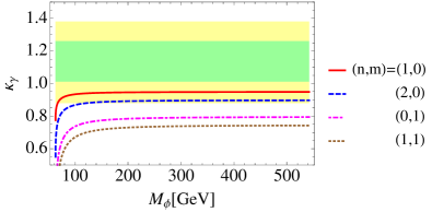
Figure 1: The prediction on $\kappa_{\gamma}$ in the models for EWSB based on CSI. The models with $(n,m)=(1,0)$, $(2,0)$, $(0,1)$ and $(1,1)$ are shown, where $n$ ($m$) is the number of singly- (doubly-) charged scalar bosons. The regions allowed by the current data from CMS k_gamma_cms are also indicated at the 1 $\sigma$ and 2$\sigma$ levels.

For the result on the $hhh$ coupling in Eq. (3), we start from discussing the case of the the SM. The quantum effect of the top quark is given approximately in Kanemura:2004mg

$$\Gamma^{\rm SM}_{hhh}\simeq\frac{3m_{h}^{2}}{v}\left(1-\frac{m_{t}^{4}}{\pi^{2}v^{2}m_{h}^{2}}+\cdots\right),$$ (21)

where the quartic power-like top mass contribution $m_{t}^{4}$ appears. These loop effects remain after the renormalization of the mass parameter ($\mu^{2}$) and the quartic coupling constant ($\lambda$) in the lowest-order effective potential

$$V(\varphi)_{\rm tree}=-\frac{1}{2}\mu^{2}\varphi^{2}+\frac{1}{4}\lambda\varphi^{4}.$$ (22)

We note that similar non-decoupling effects can also appear for bosonic loop contributions in some cases in massive extended Higgs models Kanemura:2004mg .

On the other hand, in the models for EWSB based on CSI where no mass term is introduced, the situation is drastically changed. From the effective potential in Eq. (4) with the relations in Eqs. (8) and (9), we obtain

$$\Gamma_{hhh}^{\rm CSI}\equiv\left.\frac{\partial^{3}V_{\rm eff}}{\partial\varphi^{3}}\right|_{\varphi=v}=40vB=\frac{5m_{h}^{2}}{v}.$$ (23)

Using the tree-level SM coupling $\Gamma_{hhh}^{\rm SMtree}$ ($=3m_{h}^{2}/v$), we obtain the result in Eq. (3). Because of CSI, the way of renormalization is different from the case with massive theories. Consequently, the renormalized $hhh$ coupling is expressed only in terms of $m_{h}$ and $v$. The deviation from $\Gamma_{hhh}^{\rm SMtree}$ is about +67%. This is universal for all models for EWSB based on CSI. Notice that this universality is broken in the higher order calculation, depending on details of the scalar sector of each model, although the difference is not so large, as discussed in Ref. Endo:2015ifa for a specific CSI model with O($N$) singlets. Therefore, we can test the models for EWSB based on CSI by using the $hhh$ coupling, which can be measured with the 13% accuracy at the International Linear Collider (ILC) Asner:2013psa .

Finally, some comments on the phenomenological consequences are in order. The upper bound ($\simeq 543$ GeV) on the mass of the lightest scalar boson other than $h(125)$ holds generally whatever its representation and charge. Thus, we might expect that the second scalar boson in scale invariant models for EWSB can be discovered at current and future LHC experiments. However, the detectability strongly depends on the detail of each model. By future measurements of $\kappa_{\gamma}$ at LHC Run II, the number of singly-charged scalar bosons can be determined. If at least one charged scalar boson is indicated, the possibility of a scalar sector with extra doublets would be high. For the case with a multi-doublet structure, the upper bound on $m_{1}^{\rm CSI}$ is stronger, as shown in Eq. (12). The detectability of additional scalars is very high especially when they couple to quarks and leptons as studied by many authors LHCdetect . Even if they do not have Yukawa interaction due to their inert property, we may detect them at LHC Run II Dolle:2009ft or at lepton colliders like the ILC Aoki:2013lhm . We can then finally discriminate the models from usual (massive) multi-Higgs doublet models by measuring the $hhh$ coupling at the ILC and by testing the prediction in Eq. (3). On the other hand, if future data for $\kappa_{\gamma}$ indicate that there is no charged scalar boson, the scalar sector is composed of only singlets as additional scalar fields. The testability at LHC Run II is then unclear even if their masses are light enough. Still, we can definitely test the models by measuring the $hhh$ coupling at the ILC. A detailed study is performed elsewhere hko2 .

We have discussed general aspects of models for EWSB with CSI. There is a general upper bound on the mass of the lightest scalar boson other than $h(125)$. The deviation in the $h\gamma\gamma$ coupling is mostly determined by the number of charged scalars. The deviation in the $hhh$ coupling from the SM prediction is universally about $+70$ % in these models. By using these results, the set of models based on CSI can be well tested at LHC and the ILC.

Acknowledgment: We would like to thank Michio Hashimoto, Mariko Kikuchi and Hiroaki Sugiyama for useful discussions. This work was supported, in part, by Grant-in-Aid for Scientific Research No. 23104006 (SK), Grant H2020-MSCA-RISE-2014 no. 645722 (Non Minimal Higgs) (SK), and NRF Research No. 2009-0083526 of the Republic of Korea (YO).

References

- (1) G. Aad et al. [ATLAS Collaboration], Phys. Lett. B 716, 1 (2012); S. Chatrchyan et al. [CMS Collaboration], Phys. Lett. B 716, 30 (2012).
- (2) K. A. Olive et al. [Particle Data Group Collaboration], Chin. Phys. C 38, 090001 (2014).
- (3) M. J. G. Veltman, Acta Phys. Polon. B 8, 475 (1977).
- (4) W. A. Bardeen, FERMILAB-CONF-95-391-T.
- (5) S. R. Coleman and E. J. Weinberg, Phys. Rev. D 7, 1888 (1973).
- (6) E. Gildener and S. Weinberg, Phys. Rev. D 13, 3333 (1976).
- (7) K. Funakubo, A. Kakuto and K. Takenaga, Prog. Theor. Phys. 91, 341 (1994); A. Farzinnia and J. Ren, Phys. Rev. D 90, no. 7, 075012 (2014).
- (8) K. Takenaga, Prog. Theor. Phys. 92, 987 (1994).
- (9) J. S. Lee and A. Pilaftsis, Phys. Rev. D 86, 035004 (2012).
- (10) K. Fuyuto and E. Senaha, Phys. Lett. B 747, 152 (2015).
- (11) K. Ishiwata, Phys. Lett. B 710, 134 (2012).
- (12) J. Guo and Z. Kang, Nucl. Phys. B 898, 415 (2015).
- (13) K. Endo and Y. Sumino, JHEP 1505, 030 (2015).
- (14) K. Endo and K. Ishiwata, arXiv:1507.01739 [hep-ph].
- (15) V. V. Khoze, JHEP 1311, 215 (2013).
- (16) K. Kannike, et al., JHEP 1505, 065 (2015).
- (17) R. Foot, A. Kobakhidze, K. L. McDonald and R. R. Volkas, Phys. Rev. D 76, 075014 (2007); M. Lindner, S. Schmidt and J. Smirnov, JHEP 1410, 177 (2014).
- (18) K. A. Meissner and H. Nicolai, Phys. Lett. B 648, 312 (2007); R. Foot, A. Kobakhidze and R. R. Volkas, Phys. Lett. B 655, 156 (2007); R. Foot, A. Kobakhidze, K. L. McDonald and R. R. Volkas, Phys. Rev. D 76, 075014 (2007); S. Iso, N. Okada and Y. Orikasa, Phys. Lett. B 676, 81 (2009).
- (19) G. D. Kribs, T. Plehn, M. Spannowsky and T. M. P. Tait, Phys. Rev. D 76, 075016 (2007).
- (20) M. Hashimoto, Phys. Rev. D 81, 075023 (2010).
- (21) T. Appelquist and J. Carazzone, Phys. Rev. D 11, 2856 (1975).
- (22) M. A. Shifman, A. I. Vainshtein, M. B. Voloshin and V. I. Zakharov, Sov. J. Nucl. Phys. 30, 711 (1979) [Yad. Fiz. 30, 1368 (1979)].
- (23) V. Khachatryan et al. [CMS Collaboration], Eur. Phys. J. C 75, no. 5, 212 (2015).
- (24) The ATLAS collaboration, ATLAS-CONF-2014-009, ATLAS-COM-CONF-2014-013.
- (25) S. Dawson et al., arXiv:1310.8361 [hep-ex].
- (26) S. Kanemura, Y. Okada, E. Senaha and C.-P. Yuan, Phys. Rev. D 70, 115002 (2004).
- (27) D. M. Asner et al., arXiv:1310.0763 [hep-ph].
- (28) For example, see: S. Kanemura, K. Tsumura, K. Yagyu and H. Yokoya, Phys. Rev. D 90, 075001 (2014).
- (29) E. Dolle, X. Miao, S. Su and B. Thomas, Phys. Rev. D 81, 035003 (2010).
- (30) M. Aoki, S. Kanemura and H. Yokoya, Phys. Lett. B 725, 302 (2013).
- (31) K. Hashino, S. Kanemura, Y. Orikasa, in preparation.