Unoriented knot Floer homology and the unoriented four-ball genus

Abstract.

In an earlier work, we introduced a family ${\rm{tHFK}}(K)$ of $t$-modified knot Floer homologies, defined by modifying the construction of knot Floer homology ${\mathrm{HFK}}^{-}$. The resulting groups were then used to define concordance homomorphisms $\Upsilon(t)$ indexed by $t\in[0,2]$. In the present work we elaborate on the special case $t=1$, and call the corresponding modified knot Floer homology the unoriented knot Floer homology of $K$. The corresponding concordance homomorphism when $t=1$ is denoted by $\upsilon$. Using elementary methods (based on grid diagrams and normal forms for surface cobordisms), we show that $\upsilon$ gives a lower bound for the smooth 4-dimensional crosscap number of $K$ — the minimal first Betti number of a smooth (possibly non-orientable) surface in $D^{4}$ that meets the boundary $S^{3}$ along the given knot $K$.

1. Introduction

Earlier work [16] gives a family of concordance invariants $\Upsilon_{K}(t)\in{\mathbb{R}}$ ($t\in[0,2]$), associated to a knot $K\subset S^{3}$. These numerical invariants are derived from the $t$-modified knot Floer homology ${\rm{tHFK}}(K)$ [16], defined using a modification of knot Floer homology (introduced in [20, 25]). In [16], the following properties of the invariants $\Upsilon_{K}(t)$ are verified:

1. for a connected sum $K_{1}\#K_{2}$ we have $\Upsilon_{K_{1}\#K_{2}}(t)=\Upsilon_{K_{1}}(t)+\Upsilon_{K_{2}}(t)$;

2. $\Upsilon_{K}(t)$ provides a lower bound for the slice genus $g_{s}(K)$: for $t\in[0,1]$ we have

   $$|\Upsilon_{K}(t)|\leq t\cdot g_{s}(K);$$

3. by combining Properties ($\Upsilon$-1) and ($\Upsilon$-2), for each $t\in[0,2]$ the map $K\mapsto\Upsilon_{K}(t)$ provides a homomorphism from the smooth concordance group $\mathcal{C}$ to ${\mathbb{R}}$;

4. $\Upsilon_{K}(t)=\Upsilon_{K}(2-t)$ and $\Upsilon_{K}(0)=\Upsilon_{K}(2)=0$;

5. for $t=\frac{m}{n}$ the value $\Upsilon_{K}(t)$ is in $\frac{1}{n}\mathbb{Z}$, in particular, for $t=1$ we have that $\Upsilon_{K}(1)$ is an integer.

Furthermore, for some classes of knots, $\Upsilon_{K}$ can be readily described. For an alternating knot $K$, $\Upsilon_{K}(t)$ can be described in terms of the signature and the Alexander polynomial of $K$. For a torus knot $K$ (and more generally, any knot with an $L$-space surgery) the Alexander polynomial $\Delta_{K}$ determines $\Upsilon_{K}(t)$. By partially computing these invariants in a family of satellite knots, one can show that the concordance group $\mathcal{C}$, and similarly its subgroup $\mathcal{C}_{TS}$ given by the classes of topologically slice knots, admit a direct summand isomorphic to $\mathbb{Z}^{\infty}$, reproving a recent result of Hom [6].

In this paper, we focus on one particular member of this family, where $t=1$, and study how it is related to concordance problems involving non-orientable surfaces. The $t$-modified knot Floer homology ${\rm{tHFK}}(K)$ for $t=1$ is particularly simple; it is denoted ${\mathrm{HFK}^{\prime}}(K)$, and it is called the unoriented knot Floer homology of $K$. The construction is recalled in Section 2. By construction, ${\mathrm{HFK}^{\prime}}(K)$ is a $\mathbb{Z}$-graded module over the polynomial ring $\mathbb{F}[U]$. The invariant $\upsilon(K)$ (upsilon of $K$) is defined as the value of $\Upsilon_{K}(t)$ at $t=1$: this is the maximal grading of any homogeneous, non-torsion element in the $\mathbb{F}[U]$-module ${\mathrm{HFK}^{\prime}}(K)$.

We will relate $\upsilon(K)$ with the following analogue of the slice genus. The smooth 4-dimensional crosscap number $\gamma_{4}(K)$ of a knot $K\subset S^{3}$ is the minimal

$$b_{1}(F)=b_{1}(F;\mathbb{Z}/{2}\mathbb{Z})=\dim_{\mathbb{Z}/{2}\mathbb{Z}}H_{1}(F;\mathbb{Z}/{2}\mathbb{Z})$$

of any smoothly embedded (possibly non-orientable) compact surface $(F,\partial F)$ in $(D^{4},S^{3})$ with $\partial F=F\cap S^{3}=K$. The slice genus $g_{s}(K)$ is defined similarly, only there the surfaces are required to be orientable, and we minimize the genus (which is twice the first Betti number); so clearly $\gamma_{4}(K)\leq 2g_{s}(K)$. The gap between these two invariants can be arbitrarily large: for example, for $n>0$, the $(2,2n+1)$ torus knot $T_{2,2n+1}$ has $g_{s}(T_{2,2n+1})=n$, but since this (non-slice) knot can be presented as the boundary of a Möbius band in $S^{3}$, $\gamma_{4}(T_{2,2n+1})=1$ for all $n\in{\mathbb{N}}$. For more on $\gamma_{4}$ see [3].

We wish to generalize the slice bound from $\upsilon$ (the $t=1$ specialization of Property ($\Upsilon$-2))

(1) $$|\upsilon(K)|\leq g_{s}(K)$$

to a bound on $\gamma_{4}(K)$. This generalization involves the normal Euler number of the (possibly non-orientable) surface $F$: since $F\subset D^{4}$, and the ambient manifold is oriented, a non-orientable surface $F$ has a well-defined, integer-valued self-intersection number $e(F)$, cf. Section 4.

Theorem 1.1.

Suppose that $F\subset[0,1]\times S^{3}$ is a (not necessarily orientable) smooth cobordism from the knot $K_{0}\subset\{0\}\times S^{3}$ to the knot $K_{1}\subset\{1\}\times S^{3}$. Then, we have

$$\lvert\upsilon(K_{0})-\upsilon(K_{1})+\frac{e(F)}{4}\rvert\leq\frac{b_{1}(F)}{2}.$$

Theorem 1.1 is a direct generalization of Equation (1): if $S$ is an orientable surface in $B^{4}$ meeting $S^{3}$ along $K$, remove a ball centered at a point in $S$ to obain a smooth cobordism $F$ from $K$ to the unknot $\mathcal{O}$, which has $\upsilon(\mathcal{O})=0$. Since $F$ is orientable, $e(F)=0$ and $b_{1}(F)=2g(F)$.

Theorem 1.1 is reminiscent of the “adjunction inequalities” pioneered by Kronheimer and Mrowka in gauge theory [9]; there, too, the genus bounds are corrected by a self-intersection number (though the adjunction inequalities apply to orientable surfaces).

Analogous bounds for non-orientable surfaces using a different knot concordance invariant, $d(S^{3}_{-1}(K))$ of the 3-manifold $S^{3}_{-1}(K)$ given by $(-1)$-surgery along $K$, were found by Batson [1] (and further generalized in [10]):

$$\frac{e(F)}{2}-2d(S^{3}_{-1}(K))\leq b_{1}(F).$$

Our bounds, though, are slightly different from these: unlike $d(S^{3}_{-1}(K))$, the invariant $\upsilon(K)$ is additive under connected sums.

Theorem 1.1 should be compared with bounds on the crosscap number coming from the signature $\sigma(K)$ of a knot, obtained using the Gordon-Litherland formula [4]:

(2) $$|\sigma(K)-\frac{e(F)}{2}|\leq b_{1}(F).$$

(We use the sign convention for the signature with $\sigma(T_{2,3})=-2$ for the right-handed trefoil knot $T_{2,3}$.) Combining Theorem 1.1 with Equation (2) gives:

Theorem 1.2.

For a knot $K\subset S^{3}$ , $\lvert\upsilon(K)-\frac{\sigma(K)}{2}\rvert\leq\gamma_{4}(K)$.

Proof. Suppose that $S\subset D^{4}$ is a smooth, compact surface with $\partial S=K$. Apply Theorem 1.1 for the cobordism we get from $S$ by deleting a small ball from $D^{4}$ centered on $S$, we find that $|\upsilon(K)-\frac{e(S)}{4}|\leq\frac{b_{1}(S)}{2}$. Combining this with the half of Inequality (2) we get $|\upsilon(K)-\frac{\sigma(K)}{2}|\leq b_{1}(F)$, implying the desired inequality.         

For knots and links in $S^{3}$, unoriented knot Floer homology can be set up in several ways. We could see it as a modification of the construction of knot Floer homology, as defined using pseudo-holomorphic curves; or alternatively, we can define it using grid diagrams as in [13, 14]. The equivalence of the two approaches follows from [13], and the invariance proof entirely within the grid approach is given in [14], see also [17]. In this paper, we will freely use the interchangeability of these two approaches; though, in the spirit of Sarkar’s proof of the slice bounds coming from $\tau$ [27], our proof Theorem 1.1 relies mostly on grid diagrams.

Like Sarkar’s proof of the slice genus bounds for $\tau$ in [27], the proof of Theorem 1.1 uses a normal form for knot cobordisms; for the crosscap number bound, though, we need an unorientable version, due to Kamada [7]. (The appropriately modified versions of these results will be recalled in Section 4.)

The invariant $\upsilon(K)$ can be computed for many families of knots, for which the knot Floer homology is understood. For example, following from [16], for an alternating knot $K$ we have

$$\upsilon(K)=\frac{\sigma(K)}{2}.$$

(Indeed, the same formula holds for the wider class of “quasi-alternating knots” of [23].)

We can also describe $\upsilon$ for the torus knot $T_{p,q}$. To this end, write the symmetrized Alexander polynomial $\Delta_{T_{p,q}}(t)$ of $T_{p,q}$ as

$$\Delta_{T_{p,q}}(t)=\frac{(t^{pq}-1)(t-1)}{(t^{p}-1)(t^{q}-1)}t^{-(\frac{pq-p-q-1}{2})}=\sum_{k=0}^{n}(-1)^{k}t^{\alpha_{k}},$$

where $\alpha_{i}$ is a decreasing sequence of integers. Define a corresponding sequence of numbers inductively by

$$m_{0} =0$$

$$m_{2k} =m_{2k-1}-1$$

$$m_{2k+1} =m_{2k}-2(\alpha_{2k}-\alpha_{2k+1})+1.$$

(Recall from [22] that $\widehat{\mathrm{HFK}}(T_{p,q})$ consists of the direct sum of $\mathbb{F}=\mathbb{Z}/2\mathbb{Z}$ summands supported in bigradings $\{(m_{k},\alpha_{k})\}_{k=0}^{n}$, where $m_{k}$ denotes the Maslov and $\alpha_{k}$ the Alexander gradings.) As a specialization of the computation of $\Upsilon_{K}(t)$ for torus knots [16, Theorem LABEL:Concordance:thm:TorusKnots], we get

Theorem 1.3.

For the positive $(p,q)$ torus knot $T_{p,q}$, $\upsilon(T_{p,q})=\max_{0\leq 2k\leq n}\{m_{2k}-\alpha_{2k}\}$.       

More generally, Theorem 1.3 holds for any knot in $S^{3}$ for which some positive rational surgery gives an “$L$-space” in the sense of [22]. Torus knots have this property; and other knots (e.g. certain iterated torus knots) also satisfy this condition.

For example, for the torus knot $T_{3,4}$ we have $\Delta_{T_{3,4}}(t)=t^{3}-t^{2}+1-t^{-2}+t^{-3}$, and so $\upsilon(T_{3,4})=-2$. Since $\sigma(T_{3,4})=-6$, Theorem 1.2 implies that $\gamma_{4}(T_{3,4})\geq 1$. Since the knot $T_{3,4}$ can be presented as the boundary of a Möbius band (cf. [1, Figure 4.1]), we actually get that $\gamma_{4}(T_{3,4})=1$. On the other hand, the additivity of both $\upsilon$ and $\sigma$, together with the above calculation provides

Corollary 1.4.

Consider the knot $K_{n}=\#_{n}T_{3,4}$, the $n$-fold connected sum of $T_{3,4}$. Then $\upsilon(K_{n})=-2n$ and $\sigma(K_{n})=-6n$, therefore $\gamma_{4}(K_{n})=n$.       

Note that this observation reproves [1, Theorem 2] of Batson, showing that the 4-dimensional smooth crosscap number $\gamma_{4}$ can be arbitrarily large.

The $t=1$ specialization of Property ($\Upsilon$-3) shows that $\upsilon$ induces a homomorphism from the smooth concordance group to $\mathbb{Z}$. One might wonder about the relationship between $\upsilon$ and previously existing concordance homomorphisms. Infinitely many linearly independent homomorphisms from the smooth concordance group to $\mathbb{Z}$ were constructed in work of Jen Hom [6]; but previous to this work, there were a few other concordance homomorphisms that are non-trivial on topologically slice knots. For example, there is $\tau(K)$, $\delta(K)$ (the $d$ invariant of the double branched cover of $S^{3}$ along $K$, studied by Manolescu and Owens [12]); and Rasmussen defined an invariant $s(K)$ using Khovanov homology. Computing these invariants on appropriate examples quickly leads to the following independence result:

Proposition 1.5.

The homomorphism $\upsilon$ is linearly independent from $\tau$, $\delta$, $s$, and $\sigma$.

The genus bounds obtained here are similar to earlier results; for example, those of [1] and [10] in the non-orientable case and [19] and [25] in the orientable case. Those proofs rely on the Heegard Floer homology groups for closed three-manifolds, and how these groups are related under cobordisms. By contrast, our present work relies on cominatorial decompositions of (possibly unorientable) knot cobordisms, in the spirit of Sarkar [27] (for slice genus bounds using $\tau$) and the earlier work of Rasmussen [26] (for slice genus bounds using Khovanov homology).

The paper is organized as follows. In Section 2 we provide the definition of unoriented knot Floer homology, both from the holomorphic and from the grid theoretic point of view. Since the definition relies on constructions discussed in detail elsewhere, we will make frequent references to those sources. Indeed, since ${\mathrm{HFK}^{\prime}}$ is a special case of the $t$-modified knot Floer homolog ${\rm{tHFK}}$, basic properties of unoriented knot Floer homology follow from general discussions of [16]. We define also related invariant for links, which will be needed later. In Section 3 we verify a bound on the change of $\upsilon$ under crossing changes. Although the result of Section 3 also follows from results of [16], we devoted this section to describe a more direct proof. In Section 4 we review what is needed about (orientable and non-orientable) cobordisms between knots. In particular, we quote the necessary normal form theorems. In Section 5 we give the details of the bounds on the genera and Betti numbers (in the orientable and in the non-orientable case) provided by the $\upsilon$-invariant. Although the oriented case already follows from [16], we give an alternate combinatorial proof, which is then easily modified to apply in the non-orientable case, as well. In Section 6 we give a few sample computations of ${\mathrm{HFK}^{\prime}}(K)$ and $\upsilon(K)$. In Section 7, we give a small modification of the earlier link invariant, to define unoriented link invariants.

Acknowledgements: We would like to thank Josh Batson, Ciprian Manolescu and Sucharit Sarkar for useful discussions.

2. Definition of $\upsilon$

We start by recalling the definition of unoriented knot Floer homology ${\mathrm{HFK}^{\prime}}(K)$. Although the invariant has been described in [16] (as ${\rm{tHFK}}(K)$ with $t=1$), for completeness (and since some of the constructions are needed in our later arguments) we give the details of the definition here. We start our discussion in the holomorphic context, and will turn to grid diagrams afterwards.

2.1. Unoriented knot Floer homology

Let ${\mathcal{H}}=(\Sigma,\mbox{\boldmath$\alpha$},\mbox{\boldmath$\beta$},w,z)$ be a genus-$g$ doubly pointed Heegaard diagram for a knot $K\subset S^{3}$. Let $\mathbf{S}({\mathcal{H})}$ denote the set of Heegaard Floer states for the diagram, that is, $\mathbf{S}({\mathcal{H})}$ is the set of unordered $g$-tuples $\mathbf{x}=\{x_{1},\ldots,x_{g}\}\subset\Sigma$ such that each $\alpha_{i}\in\mbox{\boldmath$\alpha$}$ and each $\beta_{j}\in\mbox{\boldmath$\beta$}$ contains a unique element of $\mathbf{x}$. There are maps $M\colon\mathbf{S}({\mathcal{H})}\to\mathbb{Z}$ (the “Maslov grading”) and $A\colon\mathbf{S}({\mathcal{H})}\to\mathbb{Z}$ (the “Alexander grading”). For the definitions and detailed discussions of these notions, see [20]; explicit formulae will be given only in the grid context.

Define the $\mathbb{Z}$-grading of the state $\mathbf{x}$ by the difference

$$\delta(\mathbf{x})=M(\mathbf{x})-A(\mathbf{x}).$$

Consider the $\mathbb{F}[U]$-module ${\mathrm{CFK}^{\prime}}({\mathcal{H}})$ freely generated by the Heegaard Floer states. We extend the $\mathbb{Z}$-grading by defining

$$\delta(U^{i}\cdot\mathbf{x})=\delta(\mathbf{x})-i.$$

(Note that this convention is compatible with the usual conventions, since multiplication by $U$ drops the Maslov grading $M$ by 2 and the Alexander grading $A$ by 1.) Equip ${\mathrm{CFK}^{\prime}}({\mathcal{H}})$ with the modified Heegaard Floer differential

(3) $$\partial\mathbf{x}=\sum_{\mathbf{y}\in\mathbf{S}({\mathcal{H})}}\sum_{\{\phi\in\pi_{2}(\mathbf{x},\mathbf{y})\mid\mu(\phi)=1\}}\#\left(\frac{\mathcal{M}(\phi)}{{\mathbb{R}}}\right)U^{n_{w}(\phi)+n_{z}(\phi)}\mathbf{y},$$

where $\mu(\phi)$ is the Maslov index (formal dimension) of the moduli space $\mathcal{M}(\phi)$ of holomorphic disks representing $\phi\in\pi_{2}(\mathbf{x},\mathbf{y})$, and $n_{w}(\phi)$ (and similarly $n_{z}(\phi)$) is the multiplicity of the domain corresponding to $\phi$ at $w$ (and $z$, resp.). The symbol $\#\left(\frac{\mathcal{M}(\phi)}{{\mathbb{R}}}\right)$ denotes the mod 2 count of elements in the quotient of the moduli space (with $\mu(\phi)=1$) by the obvious ${\mathbb{R}}$-action. For the moduli space $\mathcal{M}(\phi)$ to make sense, one needs to fix an almost complex structure on the appropriate symmetric power of the Heegaard surface — for more details see [21].

Definition 2.1.

The homology of $({\mathrm{CFK}^{\prime}}({\mathcal{H}}),\partial)$ is called the unoriented knot Floer homology of the knot $K\subset S^{3}$, and will be denoted by ${\mathrm{HFK}^{\prime}}(K)$.

In [16], we give a more general construction, parameterized by a parameter $t$. The chain complex ${\rm{tCFK}}$ is given a grading where $\mathrm{gr}_{t}(\mathbf{x})=M(\mathbf{x})-tA(\mathbf{x})$, and the differential is computed by

$$\partial_{t}\mathbf{x}=\sum_{\mathbf{y}\in\mathbf{S}}\sum_{\{\phi\in\pi_{2}(\mathbf{x},\mathbf{y})\big{|}\mu(\phi)=1\}}\#\left(\frac{\mathcal{M}(\phi)}{\mathbb{R}}\right)U^{tn_{z}(\phi)+(2-t)n_{w}(\phi)}\mathbf{y}.$$

Setting $t=1$ in this construction gives back unoriented knot complex ${\mathrm{CFK}^{\prime}}$, with the $\mathbb{Z}$-grading induced by $\delta$. Since the homology ${\rm{tHFK}}$ of ${\rm{tCFK}}$ is a knot invariant, so is the $t=1$ specialization:

Theorem 2.2.

$($[16, Theorem 1.1]$)$ The homology ${\mathrm{HFK}^{\prime}}(K)$, as a $\mathbb{Z}$-graded $\mathbb{F}[U]$-module, is an invariant of $K$.       

Remark 2.3.

The $t$-modified knot Floer homology ${\rm{tHFK}}$ is defined for all $t\in[0,2]$, and in the generic case we need to use a more complicated base ring, the ring of “long power series” (cf. [2, Section 11]). For rational $t$ (and in particular, for $t=1$), however, appropriate polynomial rings are also sufficient, as it is applied in the above definition; see [16, Proposition LABEL:Concordance:prop:SameUpsilon].

In the usual setting of knot Floer homology, by setting $U=0$ in the chain complex $\mathrm{CFK}^{-}$, and then taking homology, we get a related, simpler invariant, denoted $\widehat{\mathrm{HFK}}$.

Proposition 2.4.

The homology of ${\mathrm{CFK}^{\prime}}({\mathcal{H}})/(U=0)$ is isomorphic to $\widehat{\mathrm{HFK}}(K)$ (when in the latter group we collapse the Maslov and Alexander gradings to $\delta=M-A$).

Proof. By setting $U=0$, the differentials for both ${\mathrm{CFK}^{\prime}}/U$ and $\widehat{\mathrm{CFK}}$ count those holomorphic disks for which both $n_{w}$ and $n_{z}$ vanish, hence the resulting chain complexes are isomorphic. The isomorphism obviously respects the grading $\delta=M-A$.         

Let $\upsilon(K)$ be the maximal $\delta$-grading of any homogeneous non-torsion element in ${\mathrm{HFK}^{\prime}}(K)$:

$$\upsilon(K)=\max\{\delta(x)\mid x\in{\mathrm{HFK}^{\prime}}(K)\quad\text{homogeneous and}\quad U^{d}\cdot x\neq 0\quad\text{for all}\quad d\in{\mathbb{N}}\}.$$

Since ${\mathrm{HFK}^{\prime}}(K)$ is bounded above, to see that the above definition makes sense, we must show that there are non-torsion elements in ${\mathrm{HFK}^{\prime}}$. This could be done by appealing to the holomorphic theory; alternatively, we can appeal to Proposition 3.5 proved below. Assuming this, Theorem 2.2 immediately implies that $\upsilon(K)$ is a knot invariant. In fact, $\upsilon(K)=\Upsilon_{K}(1)$, in the notation of [16].

Remark 2.5.

In the choice of the sign of $\upsilon$ we follow the convention of [16] (in particular, $\upsilon(K)=\Upsilon_{K}(1)$). This convention differs from the convention for the $\tau$-invariant, where we have

$$\tau(K)=-\max\{A(x)\mid x\in{\mathrm{HFK}}^{-}(K)\quad\text{homogeneous and}\quad U^{d}\cdot x\neq 0\quad\text{for all}\quad d\in{\mathbb{N}}\}.$$

2.2. Formal constructions

Let $({\mathcal{C}},\partial)$ be a $\mathbb{Z}$-graded free chain complex over $\mathbb{F}[U]$ with a $\mathbb{Z}$-valued filtration, with the compatibility conditions that multiplication by $U$ drops grading by two and filtration level by one. Let $\mathbf{S}$ be a homogeneous generating set for ${\mathcal{C}}$ over $\mathbb{F}[U]$; so there are functions $M\colon\mathbf{S}\to\mathbb{Z}$ and $A\colon\mathbf{S}\to\mathbb{Z}$ so that the element $\mathbf{x}\in\mathbf{S}$ is in grading $M(\mathbf{x})$, and filtration level $A(\mathbf{x})$. We can form another complex $(C^{\prime},\partial^{\prime})$ with a $\mathbb{Z}$-grading by the following construction. $C^{\prime}$ is also generated by $\mathbf{S}$, its $\mathbb{Z}$-grading is induced by $\delta=M-A$. The differential on $C^{\prime}$ is specified by the property that $U^{m}\mathbf{y}$ appears with coefficient $1$ in the differential $\partial\mathbf{x}$ for $\mathbf{x},\mathbf{y}\in\mathbf{S}$ (so that $m=\frac{M(\mathbf{y})-M(\mathbf{x})}{2}$) if and only if $U^{\frac{\delta(\mathbf{y})-\delta(\mathbf{x})+1}{2}}\cdot\mathbf{y}$ appears with coefficient $1$ in $\partial^{\prime}\mathbf{x}$.

For example, a knot $K\subset S^{3}$ induces a filtration on ${\mathcal{CF}}^{-}(S^{3})$; if ${\mathcal{C}}$ denotes the resulting filtered chain complex, then it is straightforward to check that $C^{\prime}$ coincides with the construction of ${\mathrm{CFK}^{\prime}}(K)$ from above. (See [16, Section LABEL:Concordance:sec:Formal] for the generalization of this construction for $t\in[0,2]$.)

Constructions from knot Floer homology can be easily lifted to constructions to unoriented knot Floer homology, using the above formal trick. For example, if $({\mathcal{C}}_{1},\partial_{1})$ and $({\mathcal{C}}_{2},\partial_{2})$, are two $\mathbb{Z}$-filtered, $\mathbb{Z}$-graded free chain complexes over $\mathbb{F}[U]$, and $\phi\colon{\mathcal{C}}_{1}\to{\mathcal{C}}_{2}$ is a homotopy equivalence between them, then $\phi$ induces a homotopy equivalence $\phi^{\prime}\colon C^{\prime}_{1}\to C^{\prime}_{2}$ between their corresponding formal constructions $(C_{1}^{\prime},\partial_{1}^{\prime})$ and $(C_{2}^{\prime},\partial_{2}^{\prime})$. This is how Theorem 2.2 is derived from the invariance of the filtered chain homotopy type of ${\mathcal{CF}}^{-}(S^{3})$ with its induced filtration from $K$; see [16, Theorem 1.1].

2.3. Multi-pointed diagrams

Like knot Floer homology, unoriented knot Floer homology can be computed using Heegaard diagrams with multiple basepoints:

Definition 2.6.

Let ${\mathcal{H}}=(\Sigma,\mbox{\boldmath$\alpha$},\mbox{\boldmath$\beta$},\{w_{1},\dots,w_{n}\},\{z_{1},\dots,z_{n}\})$ be a multi-pointed Heegaard diagram for $K\subset S^{3}$. Given $\phi\in\pi_{2}(\mathbf{x},\mathbf{y})$, define its weight as

$$\mathbf{W}(\phi)=\sum_{i=1}^{n}n_{w_{i}}(\phi)+n_{z_{i}}(\phi).$$

Consider the free $\mathbb{F}[U]$-module ${\mathrm{CFK}^{\prime}}({\mathcal{H}})$ generated by the Heegaard Floer states of the Heegaard diagram ${\mathcal{H}}$, and define the boundary map as

$$\partial\mathbf{x}=\sum_{\mathbf{y}\in\mathbf{S}({\mathcal{H})}}\sum_{\{\phi\in\pi_{2}(\mathbf{x},\mathbf{y})\mid\mu(\phi)=1\}}\#\left(\frac{\mathcal{M}(\phi)}{{\mathbb{R}}}\right)U^{\mathbf{W}(\phi)}\mathbf{y}.$$

The $\delta$-grading (as the difference $M-A$ of the Maslov and Alexander gradings) extends naturally to the multi-pointed setting.

For the next theorem, it is convenient to introduce some notation. Let $V$ be the two-dimensional $\mathbb{F}$-vector space supported in $\delta$-grading equal to zero, so that if $M$ is any $\mathbb{Z}$-graded $\mathbb{F}[U]$-module, there is an isomorphism of $\mathbb{Z}$-graded $\mathbb{F}[U]$-modules:

$$M\otimes_{\mathbb{F}}V\cong M\oplus M.$$

Theorem 2.7.

The homology of $({\mathrm{CFK}^{\prime}}(\Sigma,\mbox{\boldmath$\alpha$},\mbox{\boldmath$\beta$},\mathbf{w},\mathbf{z}),\partial)$ is isomorphic to ${\mathrm{HFK}^{\prime}}(K)\otimes_{\mathbb{F}}V^{n-1}$.

Proof. There is a model for Heegaard Floer homology with multiple basepoints; see [24], and [13] for the case of knots. In this model, the chain complex ${\mathcal{C}=}{\mathcal{CF}}^{-}({\mathcal{H}})$ for ${\mathcal{CF}}^{-}(S^{3})$ (with its filtration coming from $K$) is specified as a module over $\mathbb{F}[U_{1},\dots,U_{n}]$, with differential

$$\partial\mathbf{x}=\sum_{\mathbf{y}\in\mathbf{S}({\mathcal{H})}}\sum_{\{\phi\in\pi_{2}(\mathbf{x},\mathbf{y})\mid\mu(\phi)=1\}}\#\left(\frac{\mathcal{M}(\phi)}{{\mathbb{R}}}\right)U_{1}^{n_{w_{1}}(\phi)}\cdots U_{n}^{n_{w_{n}}(\phi)}\cdot\mathbf{y}.$$

Setting all the $U_{i}$ equal to one another (and denoting the resulting formal variable by $U$), we obtain the complex $\frac{{\mathcal{C}}}{U_{1}=\dots=U_{n}}$, a $\mathbb{Z}$-filtered, $\mathbb{Z}$-graded chain complex over $\mathbb{F}[U]$, with differential given by

$$\partial\mathbf{x}=\sum_{\mathbf{y}\in\mathbf{S}({\mathcal{H})}}\sum_{\{\phi\in\pi_{2}(\mathbf{x},\mathbf{y})\mid\mu(\phi)=1\}}\#\left(\frac{\mathcal{M}(\phi)}{{\mathbb{R}}}\right)U^{n_{w_{1}}(\phi)+\dots+n_{w_{n}}(\phi)}\cdot\mathbf{y};$$

Assume for notational simplicity that $n=2$ in ${\mathcal{H}}$. In this case, we can destabilize the diagram after handleslides, to obtain a Heegaard diagram ${\mathcal{H}^{\prime}}$ for $K$ with only two basepoints $w_{1}$ and $z_{1}$. Thus, the complex ${\mathcal{C}}={\mathcal{CF}}^{-}({\mathcal{H}^{\prime}})$ is a filtered chain complex over $\mathbb{F}[U_{1}]$. We can promote this to a complex ${\mathcal{C}}[U_{2}]$ over $\mathbb{F}[U_{1},U_{2}]$, and take the filtered mapping cone of the map

$$U_{1}-U_{2}\colon{\mathcal{C}}[U_{2}]\to{\mathcal{C}}[U_{2}].$$

As in [24, Proposition 6.5] or [13, Theorem 1.1], the Heegaard moves induce a filtered homotopy equivalence of filtered complexes over $\mathbb{F}[U_{1},U_{2}]$ between the above mapping cone and ${\mathcal{CF}}^{-}({\mathcal{H}})$. Filtrations and gradings on the mapping cone are modified as follows. If $M$ is a $\mathbb{Z}$-graded $\mathbb{F}[U]$ module, let $M\llbracket k\rrbracket$ denote the same $\mathbb{F}[U]$-module, but with grading specified by

(4) $$M\llbracket k\rrbracket_{d}=M_{k+d}.$$

With this notation, the mapping cone of $U_{1}-U_{2}$ is identified with two copies of ${\mathcal{C}}[U_{2}]$; in fact, there is a $\mathbb{Z}$-graded isomorphism of $\mathbb{F}[U]$-modules

$$\mathrm{Cone}(U_{1}-U_{2})\cong{\mathcal{C}}[U_{2}]\llbracket 1\rrbracket\oplus{\mathcal{C}}[U_{2}],$$

where the first summand represents the domain of $U_{1}-U_{2}$ and the second its range. Alexader gradings are shifted similarly.

In particular, setting $U_{1}=U_{2}$, we obtain a filtered homotopy equivalence

$${\mathcal{CF}}^{-}({\mathcal{H}})\simeq{\mathcal{C}}\otimes_{\mathbb{F}}{\mathcal{V}}$$

of $\mathbb{Z}$-filtered, $\mathbb{Z}$-graded modules over $\mathbb{F}[U]$, where ${\mathcal{V}}$ is a two-dimensional $\mathbb{Z}\oplus\mathbb{Z}$-graded vector space, with one genertor in bigrading $(0,0)$ and another in bigrading $(-1,-1)$ (one of these components gives the $\mathbb{Z}$-grading and the other the $\mathbb{Z}$-filtration). It follows now that

$$({\mathcal{CF}}^{-}({\mathcal{H}}))^{\prime}\simeq({\mathcal{C}}\otimes_{\mathbb{F}}{\mathcal{V}})^{\prime}\cong{\mathcal{C}}^{\prime}\otimes_{\mathbb{F}}V.$$

The case of arbitrary $n$ is obtained by iterating the above.         

2.4. Unoriented grid homology

It follows from Theorem 2.7 that (a suitably stabilized version of) ${\mathrm{HFK}^{\prime}}(K)$ can be computed using grid diagrams. Explicitly, following the notation from [14, 17], let $\mathbb{G}$ be a grid diagram for $K$ with markings $\mathbb{X}$ and $\mathbb{O}$. Let $\mathbf{S}(\mathbb{G})$ denote the grid states of $\mathbb{G}$, i.e. the Heegaard Floer states of the Heegaard diagram induced by the the grid $\mathbb{G}$. In this picture the Maslov and Alexander gradings can be given by rather explicit formulae, as we recall below.

By considering a fundamental domain in the plane ${\mathbb{R}}^{2}$ for the grid torus, the $\mathbb{X}$- and $\mathbb{O}$-markings provide the values $M_{\mathbb{O}}(\mathbf{x})$ and $M_{\mathbb{X}}(\mathbf{x})$ for a grid state $\mathbf{x}$, as follows: For two finite sets $P,Q\subset{\mathbb{R}}^{2}$ define $\mathcal{I}(P,Q)$ to be the number of pairs $(p_{1},p_{2})\in P$ and $(q_{1},q_{2})\in Q$ with $p_{1}<q_{1}$ and $p_{2}<q_{2}$. Introduce the corresponding symmetrized function

$$\mathcal{J}(P,Q)=\frac{\mathcal{I}(P,Q)+\mathcal{I}(Q,P)}{2}.$$

We view $\mathcal{J}$ as a bilinear form, so that the expression $\mathcal{J}(P-Q,P-Q)$ is defined to mean $\mathcal{J}(P,P)-2\mathcal{J}(P,Q)+\mathcal{J}(Q,Q)$.

With this notation in place, consider the function $M_{\mathbb{O}}(\mathbf{x})$ on the grid state $\mathbf{x}$ defined by

(5) $$M_{\mathbb{O}}(\mathbf{x})=\mathcal{J}(\mathbf{x}-\mathbb{O},\mathbf{x}-\mathbb{O})+1;$$

by replacing $\mathbb{O}$ with $\mathbb{X}$ we get $M_{\mathbb{X}}(\mathbf{x})=\mathcal{J}(\mathbf{x}-\mathbb{X},\mathbf{x}-\mathbb{X})+1$. As it was verified in [14], these quantities are independent from the choice of the fundamental domain and are functions of the grid states. Indeed, the Maslov grading of $\mathbf{x}$ in the knot Floer chain complex corresponding to the grid $\mathbb{G}$ is equal to $M_{\mathbb{O}}(\mathbf{x})$, while the Alexander grading of $\mathbf{x}$ is equal to

$$A(\mathbf{x})=\frac{1}{2}(M_{\mathbb{O}}(\mathbf{x})-M_{\mathbb{X}}(\mathbf{x}))-\frac{n-1}{2},$$

where $n$ is the size (the grid index) of $\mathbb{G}$. In this setting the $\delta$-grading $\delta(\mathbf{x})=M(\mathbf{x})-A(\mathbf{x})$ can be given as

(6) $$\delta(\mathbf{x})=\frac{1}{2}(M_{\mathbb{O}}(\mathbf{x})+M_{\mathbb{X}}(\mathbf{x}))+\frac{n-1}{2}.$$

The set ${\rm{Rect}}(\mathbf{x},\mathbf{y})$ of rectangles from $\mathbf{x}$ to $\mathbf{y}$ is defined in [14]. For a rectangle $r\in{\rm{Rect}}(\mathbf{x},\mathbf{y})$ let $\mathbf{W}(r)=\#r\cap(\mathbb{X}\cup\mathbb{O})$ be the corresponding weight (as in Definition 2.6). Consider the chain complex ${\mathrm{GC}^{\prime}}(\mathbb{G})$ freely generated over $\mathbb{F}[U]$ by the grid states, endowed with the $\delta$-grading of Equation (6) and the differential

$$\partial\mathbf{x}=\sum_{\mathbf{y}\in\mathbf{S}(\mathbb{G})}\sum_{r\in{\rm{Rect}}^{0}(\mathbf{x},\mathbf{y})}U^{\mathbf{W}(r)}\mathbf{y},$$

where ${\rm{Rect}}^{0}(\mathbf{x},\mathbf{y})$ is the set of empty rectangles connecting $\mathbf{x}$ and $\mathbf{y}$ (i.e. such rectangles which do not contain in their interior any component of $\mathbf{x}$ or $\mathbf{y}$). From Theorem 2.7 and the identification of the moduli space count of the holomorphic theory with counting empty rectangles in $\mathbb{G}$ (as shown in [13]), it follows:

Corollary 2.8.

If $\mathbb{G}$ is a grid diagram for the knot $K$ of grid index $n$, then there is a $\delta$-graded $\mathbb{F}[U]$-module isomorphism

$$H_{*}({\mathrm{GC}^{\prime}}(\mathbb{G}))\cong{\mathrm{HFK}^{\prime}}(K)\otimes_{\mathbb{F}}V^{n-1},$$

where $V$ is the two-dimensional $\mathbb{F}$-vector space supported in $\delta$-grading equal to zero.       

Using grid diagrams, Corollary 2.8 (and the $\delta$-grading of $V$) gives a combinatorial description of $\upsilon(K)$.

Theorem 2.9.

The knot invariant $\upsilon(K)$ can be computed from a grid diagram $\mathbb{G}$ of the knot $K$: it is the maximal $\delta$-grading of any non-torsion homogeneous element of $H_{*}({\mathrm{GC}^{\prime}}(\mathbb{G}))$.       

In fact, one can prove that the quantity defined in the grid context is a knot invariant without appealing to the holomorphic theory, but working entirely within the context of grid diagrams. Setting this up is a straightforward adaptation of the results of [14].

2.5. The case of links

In our subsequent arguments we will need a slight extension of $\upsilon$ for links. Note that $t$-modified knot Floer homology admits a straightforward extension to links (cf. [16, Section 10]), where we use the collapsed link Floer homology $c\mathrm{HFL}^{-}$, which is a bigraded module over $\mathbb{F}[U]$.

In more detail, recall that a link $L=(L_{1},\ldots,L_{\ell})$ of $\ell$ components in $S^{3}$, equipped with an orientation $\vec{L}$, can be represented by a multi-pointed Heegaard diagram ${\mathcal{H}}=(\Sigma,\mbox{\boldmath$\alpha$},\mbox{\boldmath$\beta$},\{w_{1},z_{1}\},\ldots,\{w_{\ell},z_{\ell}\})$, where the pair $\{w_{i},z_{i}\}$ determines the $i^{th}$ component $L_{i}$. In the generalization of ${\mathrm{HFK}}^{-}$ to $\mathrm{HFL}^{-}$, a vector $(A_{1}(\mathbf{x}),\ldots,A_{\ell}(\mathbf{x}))$ of $\ell$ Alexander gradings is associated to each generator $\mathbf{x}\in{\mathbb{T}}_{\alpha}\cap{\mathbb{T}}_{\beta}$ (see [24]), and the homology has the structure of a module over the ring $\mathbb{F}[U_{1},\ldots,U_{\ell}]$. Consider next the chain complex $\mathrm{CFL}^{\prime}({\mathcal{H}})$ freely generated over $\mathbb{F}[U]$ by grid states, equipped with the differential given by

$$\partial^{\prime}\mathbf{x}=\sum_{\mathbf{y}\in\mathbf{S}({\mathcal{H})}}\sum_{\{\phi\in\pi_{2}(\mathbf{x},\mathbf{y})\mid\mu(\phi)=1\}}\#\left(\frac{\mathcal{M}(\phi)}{{\mathbb{R}}}\right)U^{\mathbf{W}(\phi)}\mathbf{y},$$

where $\mathbf{W}(\phi)=\sum_{i}n_{w_{i}}(\phi)+\sum_{i}n_{z_{i}}(\phi)$ (as in Definition 2.6). Equip $\mathrm{CFL}^{\prime}({\mathcal{H}})$ with the $\mathbb{Z}$-grading $\delta(\mathbf{x})=M(\mathbf{x})-A(\mathbf{x})$, where $A(\mathbf{x})=\sum_{i=1}^{\ell}A_{i}(\mathbf{x})$ gives another integer-valued grading. By properties of the Maslov index (see for example [24, Proposition 4.1]) and the Alexander grading (see [24, Lemma 3.11]), it follows that for any $\mathbf{x},\mathbf{y}\in\mathbf{S}({\mathcal{H})}$ and $\phi\in\pi_{2}(\mathbf{x},\mathbf{y})$,

(7) $$\delta(\mathbf{x})-\delta(\mathbf{y})=\mu(\phi)-\mathbf{W}(\phi);$$

and so the differential on $\mathrm{CFL}^{\prime}({\mathcal{H}})$ drops the $\mathbb{Z}$-grading by one.

Remark 2.10.

For links, there are several possible choices of Maslov grading. We use here the Maslov grading from [24], that is characterized by the property that the homology of the Heegaard Floer chain complex associated to ${\mathcal{H}_{S^{3}}}=(\Sigma,\mbox{\boldmath$\alpha$},\mbox{\boldmath$\beta$},\{w_{1},\dots,w_{\ell}\})$, which is isomorphic to $\mathbb{F}[U]$, has generator in Maslov grading equal to $0$.

Definition 2.11.

Let ${\mathcal{H}}=(\Sigma,\mbox{\boldmath$\alpha$},\mbox{\boldmath$\beta$},\{w_{1},z_{1}\},\dots,\{w_{\ell},z_{\ell}\})$ be a Heegaard diagram representing an oriented link $\vec{L}$. The homology of the chain complex $(\mathrm{CFL}^{\prime}({\mathcal{H}}),\partial)$ defined above (together with the $\delta$-grading) gives the unoriented link Floer homology ${\mathrm{HFL}^{\prime}}(\vec{L})$ of $\vec{L}$.

Theorem 2.12.

The unoriented link Floer homology ${\mathrm{HFL}^{\prime}}(\vec{L})$, as a $\delta$-graded $\mathbb{F}[U]$-module, is an invariant of the oriented link $\vec{L}$.

Proof. Start from the filtered link complex from [24], and set set variables $U_{1}=\dots=U_{\ell}$ to obtain a $\mathbb{Z}$-graded, $\mathbb{Z}$-filtered chain complex. According to [24], the filtered chain homotopy type of this complex is a link invariant. Applying the formal construction from Section 2.2, we arrive at the chain complex $\mathrm{CFL}^{\prime}$. As it is explained in [16, Section LABEL:Concordance:sec:Links], the application of the formal construction producing ${\rm{tHFK}}(K)$ from the filtered knot Floer complex of $K$ applies to the above chain complex over $\mathbb{F}[U]$, ultimately showing that the unoriented link Floer homology ${\mathrm{HFL}^{\prime}}(\vec{L})$ of a link $L$ is an invariant of $\vec{L}$.         

Remark 2.13.

In a Heegaard diagram $(\Sigma,\mbox{\boldmath$\alpha$},\mbox{\boldmath$\beta$},\{w_{1},z_{1}\},\dots,\{w_{\ell},z_{\ell}\})$, the orientation on $\vec{L}$ is specified by choosing the labeling of the basepoints as $w_{i}$ or $z_{i}$. The weight $\mathbf{W}(\phi)$ is independent of this choice, so the differential $\partial$ is independent of the orientation on $L$; and so, in view of Equation (7), ${\mathrm{HFL}^{\prime}}(\vec{L})$, thought of as a relatively $\mathbb{Z}$-graded module over $\mathbb{F}[U]$, is independent of the chosen orientation on $L$. The dependence of the the absolutely $\mathbb{Z}$-graded object will be described in Proposition 7.1.

Grid diagrams can be used to compute unoriented link Floer homology, as well. We define the Alexander grading for an $\ell$-component oriented link $L$ by

(8) $$A(\mathbf{x})=\frac{1}{2}(M_{\mathbb{O}}(\mathbf{x})-M_{\mathbb{X}}(\mathbf{x}))-\left(\frac{n-\ell}{2}\right)\in\mathbb{Z},$$

hence the $\delta$-grading of a grid state $\mathbf{x}$ is equal to

$$\delta(\mathbf{x})=\frac{1}{2}(M_{\mathbb{O}}(\mathbf{x})+M_{\mathbb{X}}(\mathbf{x}))+\left(\frac{n-\ell}{2}\right).$$

With this understanding, ${\mathrm{GC}^{\prime}}(\mathbb{G})$ can be defined for a grid diagram $\mathbb{G}$ representing the oriented link $\vec{L}$. For an $\ell$-component link the homology $H_{*}({\mathrm{GC}^{\prime}}(\mathbb{G}))$ is isomorphic to ${\mathrm{HFL}^{\prime}}(\vec{L})\otimes_{\mathbb{F}}V^{n-\ell}$. Indeed, the same handle sliding/destabilizing argument applies as in the proof of Theorem 2.7 until we get a Heegaard diagram with $\ell$ pairs of basepoints.

If $\vec{L}$ is an oriented link, let ${\mathcal{U}}_{m}(\vec{L})$ denote the disjoint union of $\vec{L}$ with the $m$-component unlink.

Let $W$ be the two-dimensional, $\mathbb{Z}$-graded vector space with one basis vector with degree $0$ and the other with degree $-1$, so that if $M$ is a $\mathbb{Z}$-graded module over $\mathbb{F}[U]$, there is an isomorphism

$$M\otimes_{\mathbb{F}}W\cong M\oplus M\llbracket 1\rrbracket$$

of $\mathbb{Z}$-graded modules over $\mathbb{F}[U]$, using notation from Equation (4).

Proposition 2.14.

Let $\vec{L}$ be an oriented link with $\ell$ components. Then, there is an isomorphism of $\mathbb{Z}$-graded modules over $\mathbb{F}[U]$:

$${\mathrm{HFL}^{\prime}}({\mathcal{U}}_{m}(\vec{L}))\cong{\mathrm{HFL}^{\prime}}(\vec{L})\otimes_{\mathbb{F}}W^{m}.$$

Proof. Consider $m=1$, and let ${\mathcal{H}}$ be an $\ell$-pointed Heegaard diagram for the $\ell$-component link $\vec{L}$. An $(\ell+1)$-pointed Heegaard diagram for ${\mathcal{U}}_{1}(\vec{L})$ is obtained by forming the connected sum ${\mathcal{H}^{\prime}}$ of ${\mathcal{H}}$ with a standard diagram in $S^{2}$, consisting of two embedded circles $\alpha_{\ell+1}$ and $\beta_{\ell+1}$ that intersect transversally in two points, dividing $S^{2}$ into four regions. One of the regions contains the two basepoints $w_{\ell+1}$ and $z_{\ell+1}$, its two adjacent regions are unmarked, and the fourth region is used as the connected sum point. This is the picture for an index $0$ and $3$ stabilization as in [24, Proposition 6.5]. It is similar to stabilization on a knot as in Theorem 2.7, except for the placement of the $z$ basepoints. Thus, the stabilization proof once again identifies ${\mathcal{CF}}^{-}({\mathcal{H}^{\prime}})$ with the mapping cone of

$$U_{\ell+1}-U_{\ell}\colon{\mathcal{CF}}^{-}({\mathcal{H}})\to{\mathcal{CF}}^{-}({\mathcal{H}}),$$

except that the filtration conventions are different. The two summands correspond to the two intersection points $x$ and $y$ of $\alpha_{\ell+1}$ and $\beta_{\ell+1}$. These two summands now have the same Alexander filtration levels (although their Maslov gradings are shifted as before). Thus, when we set $U_{\ell+1}=U_{\ell}$ in this complex, we obtain a filtered homotopy equivalence

$${\mathcal{CF}}^{-}({\mathcal{H}})\simeq{\mathcal{C}}\otimes_{\mathbb{F}}{\mathcal{W}}$$

of $\mathbb{Z}$-filtered, $\mathbb{Z}$-graded modules over $\mathbb{F}[U]$, where ${\mathcal{W}}$ is a two-dimensional $\mathbb{Z}\oplus\mathbb{Z}$-graded vector space, with one genertor in bigrading $(0,0)$ and another in bigrading $(-1,0)$. (Again, the first component is the Maslov grading and the second induces the Alexander filtration.) This translates into a $\mathbb{Z}$-graded quasi-isomorphism of chain complexes over $\mathbb{F}[U]$:

$${\mathrm{CFK}^{\prime}}({\mathcal{H}}^{\prime})={\mathcal{CF}}^{-}({\mathcal{H^{\prime}}})^{\prime}\simeq({\mathcal{CF}}^{-}({\mathcal{H}})\otimes_{\mathbb{F}}{\mathcal{W}})^{\prime}\cong{\mathrm{CFK}^{\prime}}({\mathcal{H}})\otimes_{\mathbb{F}}W.$$

Iterating the above result, we arrive at the proposition for arbitrary $m$.         

Corollary 2.15.

If $\vec{L}$ is the $n$-component unlink, then ${\mathrm{HFL}^{\prime}}(\vec{L})\cong\mathbb{F}[U]_{(0)}\otimes W^{n-1}$, where $W=\mathbb{F}_{(0)}\oplus\mathbb{F}_{(-1)}$.

Proof. When $\vec{L}$ is the unknot, there is a genus one diagram with one generator, with $\delta$-grading $0$. This verifies the case where $n=1$. The case where $n>1$ follows now from Proposition 2.14.         

Remark 2.16.

Although we have used the holomorphic theory to prove Propposition 2.14, a proof purely within the context of grid diagrams can also be given as in [17, Section LABEL:GridBook:sec:AddingUnknots]. Specifically, grid diagrams can be extended to give a slightly more economical description of unknotted, unlinked components. Such components are represented by a square that is simultaneously marked with an $X$ and an $O$. See Figure 1 for an extended grid diagram for the two-component link, with two generators. This picture can be used to easily verify Corollary 2.15 when $n=2$.

Figure 1. Extended grid diagram of the two-component unlink. Simple computation determines the $\delta$-gradings of the two generators shown by the diagram (indicated by the two full and the two hollow dots, respectively).

The following result will play an important role in the subsequent discussion. Given a $\mathbb{Z}$-graded chain complex $C$ over $\mathbb{F}[U]$, let ${\rm{Hom}}_{\mathbb{F}[U]}(C,\mathbb{F}[U])$ denote the chain complex of $\mathbb{F}[U]$-module homomorphisms $\phi\colon C\to\mathbb{F}[U]$, graded so that $\phi$ has degree $d$ if it sends the elements in $C_{k}$ to multiples of $U^{k+d}$.

Proposition 2.17.

If $\vec{L}$ is an oriented link with $\ell$ components and $m(\vec{L})$ is its mirror, then there is an isomorphism of graded chain complexes over $\mathbb{F}[U]$:

$${\mathrm{CFK}^{\prime}}(m(\vec{L}))\cong{\rm{Hom}}_{\mathbb{F}[U]}({\mathrm{CFK}^{\prime}}(\vec{L}),\mathbb{F}[U])\llbracket 1-\ell\rrbracket.$$

Proof. This follows from the corresponding duality under mirroring for link Floer homology; see [24, Proposition 8.3].         

From the universal coefficient theorem, it follows immediately that for a knot

(9) $$\upsilon(m(K))=-\upsilon(K);$$

see [16, Proposition LABEL:Concordance:prop:mirror] for a more general version of this statement.

3. The bound on the unknotting number

Recall that $V$ is a two-dimensional $\mathbb{Z}$-vector space supported in grading $0$, so that if $M$ is a $\mathbb{Z}$-graded module over $\mathbb{F}[U]$, then

$$M\otimes_{\mathbb{F}}V\cong M\oplus M$$

as $\mathbb{Z}$-graded modules over $\mathbb{F}[U]$. The key technical result in this section is the following:

Proposition 3.1.

Suppose that $L_{+},L_{-}$ are oriented links admitting projections which differ only at one crossing, where the projection of $L_{+}$ is a positive crossing, while for $L_{-}$ it is a negative crossing. Then there is $n\in{\mathbb{N}}$ and there are $\mathbb{F}[U]$-module maps

$$N\colon{\mathrm{HFL}^{\prime}}_{*}(L_{+})\otimes_{\mathbb{F}}V^{n}\to{\mathrm{HFL}^{\prime}}_{*}(L_{-})\otimes_{\mathbb{F}}V^{n}\qquad P\colon{\mathrm{HFL}^{\prime}}_{*}(L_{-})\otimes_{\mathbb{F}}V^{n}\to{\mathrm{HFL}^{\prime}}_{*-1}(L_{+})\otimes_{\mathbb{F}}V^{n},$$

such that $N$ preserves the $\delta$-grading, $P$ drops the $\delta$-grading by one, and furthermore $P\circ N=U$ and $N\circ P=U$.

Remark 3.2.

The same proposition holds without the stabilizing tensor products with $V$; the tensor factors appear here since we choose to use grid diagrams.

We postpone the proof of Proposition 3.1, drawing first some of its immediate consequences.

Theorem 3.3.

Suppose that $K=K_{+}$ is a given knot, together with a projection and a distingushed positive crossing, and let $K_{-}$ be the knot we get by changing that crossing. Then,

(10) $$0\leq\upsilon(K_{-})-\upsilon(K_{+})\leq 1.$$

Proof. Suppose that $x\in{\mathrm{HFK}^{\prime}}(K_{+})\otimes_{\mathbb{F}}V^{n}$ is a generator which is non-torsion and has $\delta$-grading equal to $\upsilon(K_{+})$. Then $N(x)$ is also non-torsion (since $P(N(x))=Ux$ is non-torsion), therefore $\delta(N(x))\leq\upsilon(K_{-})$. Since $N$ preserves $\delta$-grading, we get that $\upsilon(K_{+})\leq\upsilon(K_{-})$. Similarly, apply the map $P$ of Proposition 3.1 to a non-torsion element $y\in{\mathrm{HFK}^{\prime}}(K_{-})\otimes_{\mathbb{F}}V^{n}$ of $\delta$-grading $\upsilon(K_{-})$. Since $P$ shifts degree by one, a simple modification of the above argument gives $\upsilon(K_{-})-1\leq\upsilon(K_{+})$. The two arguments give Inequality (10).         

Remark 3.4.

Note that a more general version of this bound is proved in [16], where it is shown that

$$\Upsilon_{K_{+}}(t)\leq\Upsilon_{K_{-}}(t)\leq\Upsilon_{K_{+}}(t)+t$$

holds for all $t\in[0,1]$. That proof appeals to the holomorphic theory; the present proof is more in the spirit of our proof of Theorem 1.1.

It follows immediately from Theorem 3.3 that $|\upsilon(K)|\leq u(K)$: consider a minimal unknotting sequence of $K$, observe that $\upsilon$ for the unknot is $0$, and note that Theorem 3.3 shows that $\upsilon$ changes in absolute value by at most $1$ under each crossing change. This bound will be generalized in Theorem 5.6.

Before turning to the proof of Proposition 3.1, we give a further consequence of it:

Proposition 3.5.

For any $\ell$-component link $\vec{L}$, ${\mathrm{HFL}^{\prime}}(\vec{L})/\mathrm{Tors}\cong\bigoplus_{1}^{r}\mathbb{F}[U]$, where $r=2^{\ell-1}$.

Proof. Note that the maps induced by $N$ and $P$ on ${\mathrm{HFL}^{\prime}}(L)\otimes_{\mathbb{F}[U]}\mathbb{F}[U,U^{-1}]$ are isomorhpisms, since both both $P\circ N$ and $N\circ P$ are invertible on ${\mathrm{HFL}^{\prime}}(L)\otimes_{\mathbb{F}[U]}\mathbb{F}[U,U^{-1}]$. Considering a sequence of crossing changes which turn a given link $\vec{L}$ of $\ell$ components to the $\ell$-component unlink, and using Corollary 2.15, we conclude that

$${\mathrm{HFL}^{\prime}}(\vec{L})\otimes_{\mathbb{F}[U]}\mathbb{F}[U,U^{-1}]\cong\mathbb{F}[U,U^{-1}]^{r}.$$

The proposition now follows from the classification of finitely generated modules over the principal ideal domain $\mathbb{F}[U]$, according to which $({\mathrm{HFL}^{\prime}}(L)/\mathrm{Tors})\otimes_{\mathbb{F}[U]}\mathbb{F}[U,U^{-1}]\cong{\mathrm{HFL}^{\prime}}(L)\otimes_{\mathbb{F}[U]}\mathbb{F}[U,U^{-1}]$.         

Proposition 3.5 was used in the case where $\ell=1$ to verify that $\upsilon$ is well-defined for knots. The proposition also leads us to the natural extension of the $\upsilon$-invariant of knots to the case of links.

Definition 3.6.

The $\upsilon$-set of an oriented link $\vec{L}$ is a sequence of integers $\upsilon_{min}=\upsilon_{1}\leq\upsilon_{2}\leq\dots\leq\upsilon_{2^{\ell-1}}=\upsilon_{max}$ associated to $\vec{L}$ as follows. Choose a set freely generating the quotient of the $\mathbb{F}[U]$-module ${\mathrm{HFL}^{\prime}}(L)$ by its torsion part (as an $\mathbb{F}[U]$-module), with the property that each element is homogeneous with respect to the $\delta$-grading. Arrange the $\delta$-gradings of these homogeneous generators in order to obtain the $\upsilon$-set of $\vec{L}$.

It is easy to see that the above definition depends on the $\mathbb{F}[U]$-module structure of ${\mathrm{HFL}^{\prime}}(\vec{L})$; i.e. it is independent of the choice of the basis. By the invariance of unoriented link homology, it follows that the $\upsilon$-set is an invariant of $\vec{L}$. (Compare also Corollary 7.3.)

Example 3.7.

In general, we shall see in Lemma 6.3 that for any oriented link, $0\leq\upsilon_{max}(\vec{L})-\upsilon_{min}(\vec{L})\leq\ell-1$. It follows from Proposition 2.14 that if $\vec{L}$ is the $\ell$-component unlink, $\upsilon_{max}(\vec{L})=0$ and $\upsilon_{min}(\vec{L})=1-\ell$; whereas by [18, Theorem 4.1] (compare also [16, Theorem LABEL:Concordance:thm:AltKnots]), if $\vec{L}$ is a link with connected, alternating projection, then $\upsilon_{max}(\vec{L})=\upsilon_{min}(\vec{L})=\frac{\sigma-\ell+1}{2}$.

Now we return to the proof of Proposition 3.1. We will describe these maps in the grid context (explaining the presence of the stabilizations in the statement). By appropriately choosing the grid diagram $\mathbb{G}_{+}$ representing $K_{+}$, it can be assumed that a diagram $\mathbb{G}_{-}$ for $K_{-}$ is given by replacing the first column of $\mathbb{G}_{+}$ with its second column (and vice versa), see the two diagrams on the left of Figure 2. Indeed, these diagrams can be drawn on the same torus, as shown in the diagram on the right of Figure 2.

Figure 2. Grid diagrams for crossing changes. On the left we show two distinguished columns in the diagram $\mathbb{G}_{+}$ representing $K_{+}$; switching these two columns gives the diagram $\mathbb{G}_{-}$, shown in the middle, representing $K_{-}$. The diagram on the right represents both diagrams on the same torus, using two intersecting curves $\beta$ and $\gamma$.

Notice that the two new curves $\beta$ and $\gamma$ define five domains, four of which are bigons, each containing an $X$- or an $O$-marking, while the fifth one contains all the other markings. The two bigons containing the $X$-markings meet at $t\in\beta\cap\gamma$, while the intersection of the two curves above the top $X$-marking is $s$, cf. Figure 2.

The maps $N$ and $P$ are defined by counting empty pentagons (in the sense of [14, Section 3.1]). More precisely, suppose that $\mathbf{x}_{+}$ is a generator of ${\mathrm{GC}^{\prime}}(\mathbb{G}_{+})$ and $\mathbf{x}_{-}$ is a generator of ${\mathrm{GC}^{\prime}}(\mathbb{G}_{-})$. Then the $\mathbb{F}[U]$-module maps $N$ and $P$ on these chains are defined as

$$N(\mathbf{x}_{+})=\sum_{\mathbf{y}_{-}\in\mathbf{S}(\mathbb{G}_{-})}\sum_{p\in{\rm{Pent}}^{0}_{s}(\mathbf{x}_{+},\mathbf{y}_{-})}U^{\mathbf{W}(p)}\cdot\mathbf{y}_{-},$$

$$P(\mathbf{x}_{-})=\sum_{\mathbf{y}_{+}\in\mathbf{S}(\mathbb{G}_{+})}\sum_{p\in{\rm{Pent}}^{0}_{t}(\mathbf{x}_{-},\mathbf{y}_{+})}U^{\mathbf{W}(p)}\cdot\mathbf{y}_{+},$$

where ${\rm{Pent}}^{0}_{s}(\mathbf{x}_{+},\mathbf{y}_{-})$ and ${\rm{Pent}}^{0}_{t}(\mathbf{x}_{-},\mathbf{y}_{+})$ denote the sets of empty pentagons with corner at $s$ and $t$, respectively, connecting the indicated grid states. (The quantity $\mathbf{W}(p)$ for an empty pentagon is defined as the corresponding weight has been defined for rectangles: $\mathbf{W}(p)=\#p\cap(\mathbb{X}\cup\mathbb{O})$.)

Proof  of Proposition 3.1. Consider the module maps $N$ and $P$ defined above. The usual decomposition argument examining the interaction of rectangles (contributing to the boundary maps of the chain complexes) and the pentagons defining $P$ and $N$ (cf. [14, Section 3.1]) shows that both maps are chain maps, inducing the maps (denoted by the same symbols) of the proposition on the stabilized unoriented link Floer homology groups. In a similar manner (by adapting the arguments of [14, Section 3.1]) we can verify the claimed degree shifts.

To verify $N\circ P=U$ (and similarly, $P\circ N=U$) we construct maps

$$H_{+} \colon{\mathrm{GC}^{\prime}}_{d}(\mathbb{G}_{+})\to{\mathrm{GC}^{\prime}}_{d}(\mathbb{G}_{+})$$

$$H_{-} \colon{\mathrm{GC}^{\prime}}_{d}(\mathbb{G}_{-})\to{\mathrm{GC}^{\prime}}_{d}(\mathbb{G}_{-}).$$

satisfying

(11) $$\partial\circ H_{+}+H_{+}\circ\partial =P\circ N+U$$

(12) $$\partial\circ H_{-}+H_{-}\circ\partial =N\circ P+U,$$

where $U$ denotes the operator of multiplication by $U$ in the appropriate $\mathbb{F}[U]$-module. Indeed, consider the set ${\rm{Hex}}^{0}_{t,s}(\mathbf{x}_{+},\mathbf{y}_{+})$ of empty hexagons (as in [14, Section 3.1]) connecting the grid states $\mathbf{x}_{+},\mathbf{y}_{+}\in\mathbf{S}(\mathbb{G}_{+})$, having two vertices at $t$ and $s$ (in this order). Define ${\rm{Hex}}^{0}_{s,t}(\mathbf{x}_{-},\mathbf{y}_{-})$ similarly (for grid states $\mathbf{x}_{-},\mathbf{y}_{-}$ of $\mathbb{G}_{-}$). Then the definitions

$$H_{+}(\mathbf{x}_{+})=\sum_{\mathbf{y}\in\mathbf{S}(\mathbb{G}_{+})}\sum_{h\in{\rm{Hex}}^{0}_{t,s}(\mathbf{x},\mathbf{y})}U^{\mathbf{W}(h)}\cdot\mathbf{y}_{+}$$

$$H_{-}(\mathbf{x}_{-})=\sum_{\mathbf{y}\in\mathbf{S}(\mathbb{G}_{-})}\sum_{h\in{\rm{Hex}}^{0}_{s,t}(\mathbf{x},\mathbf{y})}U^{\mathbf{W}(h)}\cdot\mathbf{y}_{-}$$

provide the required maps. Once again, the simple adaptation of [14, Section 3.1] verifies the required identities of Equations (11) and (12). Indeed, by examining the various decompositions of the composition of a hexagon (counted in $H_{\pm}$) and a rectangle (counted in $\partial$), we either get an alternate decomposition of the composite domain as a rectangle and a hexagon, or the composition of two pentagons (counted in $P\circ N$ or in $N\circ P$). The only exception is the thin annular hexagon (containing no complete circle, hence component in its interior) wrapping aroung the torus. These domains do not admit alternate decompositions; on the other hand, the position of the markings now implies that these domains contain an $O$-marking, hence they provide an additive term of multiplication by $U$, exactly as stated.     

4. Knot cobordisms

Let $F$ be an embedded surface in $[0,1]\times S^{3}$, which meets $\{0\}\times S^{3}$ and $\{1\}\times S^{3}$ in knots $K_{0}$ and $K_{1}$, respectively. The surface $F$ has an Euler number $e(F)$, defined as follows. Fix the orientation on $[0,1]\times S^{3}$ we get by concatenating the canonical orientation of $[0,1]$ with an orientation of $S^{3}$. Take a local orientation system on $F$, and let $F^{\prime}$ be a small push-off of $F$, giving the Seifert framings of $K_{0}$ and $K_{1}$ in $\{0\}\times S^{3}$ and in $\{1\}\times S^{3}$, respectively. A local orientation system on $F^{\prime}$ is induced by the given local orientation system of $F$. At each (transverse) intersection point $p\in F\cap F^{\prime}$, compare the induced orientation from $T_{p}F\oplus T_{p}F^{\prime}$ with the orientation on $T_{p}([0,1]\times S^{3})$ and get a sign $\pm 1$, called the local self-intersection number at $p$. Adding up these contributions at each intersection point gives the Euler number $e(F)$. (Equivalently, pass to the orientable double cover ${\widetilde{F}}$, pull back the normal bundle of $F$, along with its trivialization at $\partial F$. Half of the relative Euler number of this oriented $2$-plane bundle is the Euler number of $F$.) When $F$ is orientable, the quantity defined in this manner vanishes.

Remark 4.1.

Notice that if we turn the cobordism upside down, then we reverse the orientation both on the $[0,1]$- and the $S^{3}$-factors, hence the Euler number remains unchanged. If the surface $F$ is embedded in $S^{3}=\{1\}\times S^{3}$, we can make it a cobordism in two different ways: we can push either end of the cobordism into $\{0\}\times S^{3}$ and keep the other one in $\{1\}\times S^{3}$. The resulting Euler numbers of the two cobordisms will be opposites of each other: the two presentations correspond to the two different orientations on $[0,1]$ (while keeping the orientation of $S^{3}$ unchanged). Therefore, when we consider an unorientable cobordism in $S^{3}$, its Euler number makes sense only after we specify a direction on the cobordism, that is, if we specify an incoming and an outgoing end of the surface (viewed as a 2-dimensional cobordism in $[0,1]\times S^{3}$).

A saddle move on a link $L$ is specified by an embedded rectangle $B$ (which we call a “band”) in $S^{3}$ with opposite sides on $L$. A new link $L^{\prime}$ is obtained by deleting the two sides of the band in $L$ and replacing them with the other two sides of the band. Fix an orientation $\vec{L}$ on $L$. A saddle move is called oriented if the orientations of the two arcs in $L$ are compatible with the boundary orientation of the band; otherwise, it is called an unorientable saddle. An unorientable saddle specifies a cobordism $F$ from $L$ to $L^{\prime}$ with $b_{1}(F,\mathbb{Z}/{2}\mathbb{Z})=1$. We will always apply the convention that, when viewing the saddle band as a cobordism, the original link $L$ is in $\{0\}\times S^{3}$ (that is, $L$ is the incoming end) and the resulting link $L^{\prime}$ is in $\{1\}\times S^{3}$ (so $L^{\prime}$ is the outgoing end).

If $L=K$ is a knot, an unoriented saddle move gives rise to another knot $L^{\prime}=K^{\prime}$. For an unorientable saddle, the relative Euler number can be computed as follows.

Lemma 4.2.

Suppose that $B$ is an unorientable saddle band from the knot $K$ to $K^{\prime}$. Choose a nonzero section $s$ of the normal bundle of the band $B$, and choose a framing $\lambda$ of $K$ which agrees with $s$ along the two arcs in $B\cap K$. Let $\lambda^{\prime}$ be the induced framing of $K^{\prime}$. Then,

(13) $$e(B)={\ell k}(K,\lambda)-{\ell k}(K^{\prime},\lambda^{\prime}),$$

where here, for example, ${\ell k}(K,\lambda)$ denotes the linking number of $K$ with the push-off of $K$ specified by the framing $\lambda$. (As before, $K$ is the incoming and $K^{\prime}$ is the outgoing end of the cobordism.)

Proof. From the definition of the linking number, it is clear that the Euler number of the band is equal to the difference of the two linking numbers. Indeed, by considering a nowhere zero section over $B$, the difference of the linking numbers determines its difference from a section with possible zeros, but which induces the Seifert framings at the two ends.

The sign in the formula, however, deserves a short explanation. For simplicity, assume that $K^{\prime}$ bounds a surface $F$ with Euler number $e(F)$. (The case of cobordisms follows along a similar logic.) In computing the Euler number consider a nonvanishing section of the normal bundle along $F$ and consider the induced framing (still denoted by $\lambda^{\prime}$) along $K^{\prime}$. If we take the trivial cobordism $W$, now from $K^{\prime}=K^{\prime}_{0}\subset\{0\}\times S^{3}$ to $K^{\prime}_{1}\subset\{1\}\times S^{3}$ with a section of the normal bundle which interpolates between the framing $\lambda^{\prime}$ on $K^{\prime}_{0}$ and the Seifert framing on $K_{1}^{\prime}$, then this section will have zeros. Indeed, the (signed) number of zeros is exactly the Euler number of the surface $F$ (since together with the topologically trivial collar between $K^{\prime}=K_{0}^{\prime}$ and $K_{1}^{\prime}$ and the section there, we have a section inducing the Seifert framing). On the other hand, the number of zeros along $W$ can be easily computed: consider a Seifert surface of $K_{0}^{\prime}$, push it into $D^{4}$ to get a surface $W^{\prime}$ and glue it to $W$. Extend the framing $\lambda^{\prime}$ to a section $\sigma$ of the normal bundle of $W^{\prime}$. Clearly, the number of zeros of $\sigma$ is ${\ell k}(K^{\prime},\lambda^{\prime})$ (following from the definition of the linking number), while if we glue $\sigma$ to our section over $W$ we get a section of $W^{\prime}\cup W$ inducing the Seifert framing on its boundary, hence the sum of zeros of this section is zero. This shows that over $W$ the signed number of zeros (and hence the Euler number $e(F)$) is $-{\ell k}(K^{\prime},\lambda^{\prime})$, justifying the formula of Equation (13), and concluding the proof of the lemma.         

The above formula can be given in explicit terms if the saddle band is related to an unoriented resolution of a crossing. Fix a diagram ${\mathcal{D}}$ of a knot $K$, and choose a crossing in the projection. Suppose that the unoriented resolution of that crossing gives an unorientable saddle $B$ (embedded in $S^{3}$) that connects $K$ to the result $K^{\prime}$ of the resolution, see Figure 3. (Once again, we assume that, as a cobordism, $B$ is from $K$ to $K^{\prime}$.)

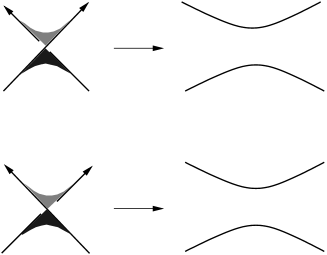
Figure 3. Unorientable saddle band attachment at a crossing of a diagram. In the top diagram the band resolves a positive crossing, in the bottom diagram it resolves a negative crossing.

Recall that the writhe $\mathrm{wr}({\mathcal{D}})$ of the diagram ${\mathcal{D}}$ is defined as the sum of the signs of the crossings. Alternatively, take $\lambda_{bb}$ to be the framing of $K$ given by the diagram (called the blackboard framing): move each point of the knot up (parallel to the projection) to get $\lambda_{bb}$. Then $\mathrm{wr}({\mathcal{D}})={\ell k}(K,\lambda_{bb})$. The writhe $\mathrm{wr}({\mathcal{D}})$ (and similarly $\lambda_{bb}$) depends on the chosen diagram; it is not an invariant of $K$. On the other hand, for a projection ${\mathcal{D}}$ of a knot the writhe $\mathrm{wr}({\mathcal{D}})$ is independent of the chosen orientation on the knot.

Lemma 4.3.

Let $K_{1}$ be a given knot, together with a diagram ${\mathcal{D}}_{1}$ and $B$ an unorientable saddle band coming from an unoriented resolution of a crossing of ${\mathcal{D}}_{1}$. Let $K_{2}$ denote the knot given by the resolution, together with the resulting diagram ${\mathcal{D}}_{2}$ of it. Then,

$$e(B)=\mathrm{wr}({\mathcal{D}}_{1})-\mathrm{wr}({\mathcal{D}}_{2})+\epsilon,$$

where

• $\epsilon=+1$ if the resolution eliminates a positive crossing in ${\mathcal{D}}_{1}$

• $\epsilon=-1$ if the resolution eliminates a negative crossing in ${\mathcal{D}}_{1}$.

Proof. Move the saddle band slightly up on the knot to achieve that it becomes embedded in the plane, cf. Figure 4.

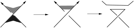
Figure 4. Moving the saddle band. By slighly pushing the band up on the knot, we can assume that it is embedded by the projection in the plane.

In this picture the vector field pointing upwards (parallel to the projection) will give a nowhere zero vector field in the normal bundle of the band $B$, restricting to two framings along $K_{1}$ and $K_{2}$. The diagram for $K_{1}$ is still ${\mathcal{D}}_{1}$, but the diagram ${\mathcal{D}}_{2}^{\prime}$ we get for $K_{2}$ is different from ${\mathcal{D}}_{2}$. Since the chosen vector field induces the blackboard framings on the two diagrams, the formula of Equation (13) determines the Euler number $e(B)$:

(14) $$e(B)=\mathrm{wr}({\mathcal{D}}_{1})-\mathrm{wr}({\mathcal{D}}_{2}^{\prime}).$$

It is easy to see that the diagram ${\mathcal{D}}_{2}^{\prime}$ for $K_{2}$ differs from ${\mathcal{D}}_{2}$ by a Reidemeister 1 move of introducing an extra crossing (cf. the right-most diagram of Figure 4). Since the two strands in this crossing were oriented so that after the resolution these orientations are in conflict (since we consider the unoriented resolution), we need to change the orientation on one of the strands, reversing the sign of the crossing. Hence $\mathrm{wr}({\mathcal{D}}_{2})=\mathrm{wr}({\mathcal{D}}_{2}^{\prime})+\epsilon$, which, combined with Equation (14) provides the result.         

Remark 4.4.

In the same vein we can examine unorientable saddle band attachments which create a new crossing in a diagram. The formula for computing the Euler number is similar, with the rule that $\epsilon$ is equal to $-1$ if the saddle introduces a positive crossing in ${\mathcal{D}}_{2}$ and is $+1$ if it introduces a negative crossing in ${\mathcal{D}}_{2}$. The argument is essentially the same as the proof given above.

Our slice bounds in Section 5 will depend on “normal form” theorems for knot cobordisms. We will handle the orientable and non-orientable situations slightly differently. The relevant theorem in the orientable case is from [8] and its non-orientable version is due to Kamada [7]. To state these in the form we will use later, recall that ${\mathcal{U}}_{n}(K)$ denotes the link obtained by adding $n$ unknotted, unlinked components to a knot $K$.

Theorem 4.5.

$($Orientable normal form, [8]$)$ Suppose that there is an orientable surface $F\subset[0,1]\times S^{3}$ of genus $g$, which is a cobordism from $K_{1}$ to $K_{2}$. Then, there are integers $c$ and $d$, and knots $K_{1}^{\prime}$ and $K_{2}^{\prime}$ with the following properties:

• $K_{1}^{\prime}$ is gotten from ${\mathcal{U}}_{c}(K_{1})$ by adding exactly $c$ orientable saddles.

• $K_{2}$ is gotten from ${\mathcal{U}}_{d}(K_{2}^{\prime})$ by adding exactly $d$ orientable saddles.

• There is a cobordism $F^{\prime}$ of genus $g$ from $K_{1}^{\prime}$ to $K_{2}^{\prime}$ which is composed by the addition of $2g$ orientable saddles.       

Theorem 4.6.

$($Non-orientable normal form, [7]$)$ Suppose that there is a non-orientable surface $F\subset[0,1]\times S^{3}$, which is a cobordism from $K_{1}$ to $K_{2}$. Then, there are integers $c$ and $d$, and knots $K_{1}^{\prime}$ and $K_{2}^{\prime}$ with the following properties:

• $K_{1}^{\prime}$ is gotten from ${\mathcal{U}}_{c}(K_{1})$ by adding exactly $c$ orientable saddles.

• $K_{2}$ is gotten from ${\mathcal{U}}_{d}(K_{2}^{\prime})$ by adding exactly $d$ orientable saddles.

• There is a cobordism $F^{\prime}$ from $K_{1}^{\prime}$ to $K_{2}^{\prime}$ composed of $b=b_{1}(F^{\prime})=b_{1}(F)$ non-orientable saddles, and with $e(F^{\prime})=e(F)$.       

Remark 4.7.

Although in [7] the normal form theorem is stated for embedded, non-orientable closed surfaces, the exact same argument provides the result above for cobordisms between knots.

The outline of the proofs of the normal form theorems goes as follows: restrict the projection function $[0,1]\times S^{3}\to[0,1]$ to the cobordims $F$. By generic position we can assume that the result is a Morse function, and it is easy to isotope $F$ so that (when increasing $t$ in $[0,1]$) we encounter first the index-0 critical points, then the index-1 and finally the index-2 critical points. With a possible further isotopy we can arrange that index-1 critical points correspond to the same value. By considering first those index-1 critical points for which the corresponding bands make the ascending disks of the index-0 handles and $K_{1}$ connected (and repeating the same process for the 2-handles, now upside down), we get the desired form of the theorem. Notice that in the non-orientable case the equality $e(F)=e(F^{\prime})$ follows trivially from the fact that the subsurface given by the 0-handles and the orientable saddles is orientable, hence has vanishing Euler number. In the non-orientable case further handle slides are needed to assure that all 1-handle attachments between the knots $K_{1}^{\prime}$ and $K_{2}^{\prime}$ are non-orientable. For more on Theorem 4.5 see [17, Appendix B.5].

5. Slice bounds from $\upsilon$

The proofs of the estimates on the genera of orientable and first Betti numbers of non-orientable slice surfaces for a knot $K$ will both rely on the normal form theorems of knot cobordisms discussed in the previous section. We start with the discussion of the orientable case, and turn to the non-orientable case afterwards.

5.1. Orientable slice bounds from $\upsilon$

In order to prove the bound provided by $\upsilon(K)$ on the oriented slice genus $g_{s}(K)$ of $K$, we need to understand how the invariant changes under oriented saddle moves. For this, the following proposition will be of crucial importance.

Proposition 5.1.

Let $L$ and $L^{\prime}$ be two links, related by an oriented saddle move, and suppose that $L^{\prime}$ has one more component than $L$. Then, there is an integer $n\in{\mathbb{N}}$ and there are $\mathbb{F}[U]$-module maps

$$\sigma \colon{\mathrm{HFL}^{\prime}}(L)\otimes_{\mathbb{F}}V^{n}\to{\mathrm{HFL}^{\prime}}(L^{\prime})\otimes_{\mathbb{F}}V^{n-1}$$

$$\mu \colon{\mathrm{HFL}^{\prime}}(L^{\prime})\otimes_{\mathbb{F}}V^{n-1}\to{\mathrm{HFL}^{\prime}}(L)\otimes_{\mathbb{F}}V^{n}$$

with the following properties:

• $V$ is a two-dimensional $\mathbb{F}$-vector space in $\delta$-grading 0,

• $\sigma$ drops $\delta$-grading by one,

• $\mu$ preserves $\delta$-grading,

• $\mu\circ\sigma$ is multiplication by $U$,

• $\sigma\circ\mu$ is multiplication by $U$.

The map $\sigma$ will be referred to as the split map and $\mu$ as the merge map. We prove the above proposition after establishing its key consequence:

Theorem 5.2.

Let $L$ and $L^{\prime}$ be two links which differ by an oriented saddle move, and suppose that $L^{\prime}$ has one more component than $L$. Then,

(15) $$\upsilon_{max}(L)-1 \leq\upsilon_{max}(L^{\prime})\leq\upsilon_{max}(L)$$

(16) $$\upsilon_{min}(L)-1 \leq\upsilon_{min}(L^{\prime})\leq\upsilon_{min}(L).$$

Proof. Consider a homogeneous non-torsion element $x\in{\mathrm{HFL}^{\prime}}(L)\otimes V^{n}$ with maximal $\delta$-grading, i.e. $\delta(x)=\upsilon_{max}(L)$. By Proposition 5.1, its image $\sigma(x)$ is non-torsion, and is of $\delta$-grading $\upsilon_{max}(L)-1$, hence $\upsilon_{max}(L)-1\leq\upsilon_{max}(L^{\prime})$. Similarly, if $y\in{\mathrm{HFL}^{\prime}}(L^{\prime})\otimes V^{n-1}$ is a non-torsion element with maximal $\delta$-grading $\upsilon_{max}(L^{\prime})$, then its image $\mu(y)$ has $\delta$-grading $\upsilon_{max}(L^{\prime})$, and it is non-torsion, so $\upsilon_{max}(L^{\prime})\leq\upsilon_{max}(L)$, verifying Inequality (15).

Inequality (16) is obtained via a similar logic. The details, however, are slightly more involved, since the definition of $\upsilon_{min}(L)$ is not as straightforward as the definition of $\upsilon_{max}(L)$. Suppose that $a\in{\mathrm{HFL}^{\prime}}(L)\otimes V^{n}$ is an element generating a free summand in $({\mathrm{HFL}^{\prime}}(L)/\mathrm{Tors})\otimes V^{n}$ with $\delta$-grading $\upsilon_{min}(L)$. Then $\sigma(a)$ has $\delta$-grading $\upsilon_{min}(L)-1$, and it either generates a free summand in $({\mathrm{HFL}^{\prime}}(L^{\prime})/\mathrm{Tors})\otimes V^{n-1}$ or it is $U$-times such a generator. Indeed, if $\sigma(a)=U^{2}h$ for some element $h$, then $\mu(\sigma(a))=Ua$ is equal to $U^{2}\mu(h)$, and since multiplication by $U$ is injective on the factor $({\mathrm{HFL}^{\prime}}(L)/\mathrm{Tors})\otimes V^{n}$, we would get $a=U\mu(h)$, contradicting the choice of $a$ as a generator. Hence from the two possibilities (according to whether $\sigma(a)$ is a generator, or $U$-times a generator) we get two inequalities, and $\upsilon_{min}(L^{\prime})\leq\upsilon_{min}(L)$ holds in both cases. With the same logic, starting now with a generator of $({\mathrm{HFL}^{\prime}}(L^{\prime})/\mathrm{Tors})\otimes V^{n-1}$ of $\delta$-grading $\upsilon_{min}(L^{\prime})$ and applying $\mu$, we get $\upsilon_{min}(L)\leq\upsilon_{min}(L^{\prime})+1$, concluding the proof.         

We prove Proposition 5.1 using grid diagrams.

Proof of Proposition 5.1. It is not hard to see that any oriented band from $L$ to $L^{\prime}$ can be represented by the following move: there is a grid diagram $\mathbb{G}$ for $L$ such that by switching the $O$-markings in the first two columns (as shown by Figure 5) we get the grid diagram $\mathbb{G}^{\prime}$ representing $L^{\prime}$. Let $n+\ell$ be equal to the grid index of $\mathbb{G}$ (and so of $\mathbb{G}^{\prime}$), where $L$ has $\ell$ components (and so $L^{\prime}$ has $\ell+1$ components by our assumption). Let $O_{1}$ denote the $O$-marking in the first column of $\mathbb{G}$ and $O_{2}$ the $O$-marking in the second column of the same grid diagram. After switching them, the new $O$-markings will be denoted by $O_{1}^{\prime}$ and $O_{2}^{\prime}$, respectively, see Figure 5.

Figure 5. Grid diagrams for an oriented saddle move. The left diagram is the first two columns of a grid diagram representing $L$, and we get a diagram for $L^{\prime}$ by switching the $O$-markings of these columns (given on the right). The figure also shows the arc ${\mathbf{A}}$ by the thicker segment. The complement of ${\mathbf{A}}$ in the circle is ${\mathbf{B}}$.

The grid states of $\mathbb{G}$ and of $\mathbb{G}^{\prime}$ are naturally identified, and can be classified into two types. This classification is based on the position of the coordinate occupying the circle between the first and second columns. Indeed, the two $O$-markings partition this circle into two intervals, one of which (call it ${\mathbf{B}}$) passes by the two $X$-markings, while the other one (which is, in some sense ’between the $O$-s’) is called ${\mathbf{A}}$, see Figure 5 where the interval ${\mathbf{A}}$ is indicated. Now a grid state $\mathbf{x}$ is of type ${\mathbf{A}}$ if the coordinate of $\mathbf{x}$ between the first and second columns is in ${\mathbf{A}}$; otherwise $\mathbf{x}$ is of type ${\mathbf{B}}$.

We define the $\mathbb{F}[U]$-module maps $\sigma\colon{\mathrm{GC}^{\prime}}(\mathbb{G})\to{\mathrm{GC}^{\prime}}(\mathbb{G}^{\prime})$ and $\mu\colon{\mathrm{GC}^{\prime}}(\mathbb{G}^{\prime})\to{\mathrm{GC}^{\prime}}(\mathbb{G})$ as follows: for a grid state $\mathbf{x}\in{\mathbf{A}}$ consider

$$\sigma(\mathbf{x})=U\cdot\mathbf{x},\quad\mu(\mathbf{x})=\mathbf{x},$$

and for a grid state $\mathbf{x}\in{\mathbf{B}}$ take

$$\sigma(\mathbf{x})=\mathbf{x},\qquad\mu(\mathbf{x})=U\cdot\mathbf{x}.$$

The definition immediately implies that both $\sigma\circ\mu$ and $\mu\circ\sigma$ are multiplications by $U$.

The proposition is proved once we show that the maps defined above on the chain level are chain maps, which have the required behavior on the $\delta$-grading. Indeed, then the maps appearing in the statement of the proposition will be the maps induced by these chain maps on homology.

First we argue that the maps $\sigma$ and $\mu$ are chain maps; below we will concentrate on the map $\sigma$. To this end, consider a rectangle $r$ connecting two grid states $\mathbf{x}$ and $\mathbf{y}$ in $\mathbb{G}$. Note that the $\mathbb{X}$-markings in $\mathbb{G}$ and in $\mathbb{G}^{\prime}$ coincide, hence we only need to examine the change of interaction of $r$ with $\mathbb{O}$ and $\mathbb{O}^{\prime}$. If both grid states $\mathbf{x},\mathbf{y}$ are from ${\mathbf{B}}$, then the rectangle $r$ contains $\{O_{1},O_{2}\}$ with the same multiplicity as it contains $\{O_{1}^{\prime},O_{2}^{\prime}\}$, viewed as a rectangle in either $\mathbb{G}$ or $\mathbb{G}^{\prime}$. The same holds if $\mathbf{x}$ and $\mathbf{y}$ are both in ${\mathbf{A}}$. If $\mathbf{x}\in{\mathbf{A}}$ and $\mathbf{y}\in{\mathbf{B}}$, then the rectangle $r$, thought of as a rectangle in $\mathbb{G}$, contains exactly one of $O_{1}$ or $O_{2}$, but it does not contain either of $O_{1}^{\prime}$ or $O_{2}^{\prime}$, i.e. the contribution of $r$ to $\partial\mathbf{x}$ contains $\mathbf{y}$ with an extra factor of $U$ not appearing in the contribution of $r$ to $\partial^{\prime}\mathbf{x}$. The definition of $\sigma$ compensates for this difference, verifying $\partial^{\prime}\circ\sigma(\mathbf{x})=\sigma\circ\partial(\mathbf{x})$ when $\mathbf{x}\in{\mathbf{A}}$. Similarly, in the case where $\mathbf{x}\in{\mathbf{B}}$ and $\mathbf{y}\in{\mathbf{A}}$, $r$ contains neither of $O_{1}$ or $O_{2}$, but it does contain exactly one of $O_{1}^{\prime}$ or $O_{2}^{\prime}$, so $r$ contributes an extra $U$ factor in $\partial^{\prime}(\mathbf{x})$ which it does not in $\partial(\mathbf{x})$. This discrepancy is also compensated for in the definition of $\sigma$. The map $\mu$ is a chain map by the same logic.

In comparing the $\delta$-gradings of $\mathbf{x}$ in $\mathbb{G}$ and in $\mathbb{G}^{\prime}$, we first verify that for an element $\mathbf{x}\in{\mathbf{A}}$ we have $M_{\mathbb{O}^{\prime}}(\mathbf{x})=M_{\mathbb{O}}(\mathbf{x})+1$, while for $\mathbf{x}\in{\mathbf{B}}$, $M_{\mathbb{O}^{\prime}}(\mathbf{x})=M_{\mathbb{O}}(\mathbf{x})-1$. Indeed, $\mathcal{I}(\mathbf{x},\mathbf{x})$ is the same in both diagrams, while (using Figure 5) it is easy to see that $\mathcal{I}(\mathbb{O}^{\prime},\mathbb{O}^{\prime})=\mathcal{I}(\mathbb{O},\mathbb{O})-1$. For the mixed terms $\mathcal{I}(\mathbb{O}^{\prime},\mathbf{x})=\mathcal{I}(\mathbb{O},\mathbf{x})$ and $\mathcal{I}(\mathbf{x},\mathbb{O}^{\prime})=\mathcal{I}(\mathbf{x},\mathbb{O})$ for $\mathbf{x}\in{\mathbf{B}}$, while $\mathcal{I}(\mathbb{O}^{\prime},\mathbf{x})=\mathcal{I}(\mathbb{O},\mathbf{x})-1$ and $\mathcal{I}(\mathbf{x},\mathbb{O}^{\prime})=\mathcal{I}(\mathbf{x},\mathbb{O})-1$ for a grid state $\mathbf{x}\in{\mathbf{A}}$. Since $\mathbb{X}=\mathbb{X}^{\prime}$, we get that $\delta_{\mathbb{G}}(\mathbf{x})=\frac{1}{2}(M_{\mathbb{O}}(\mathbf{x})+M_{\mathbb{X}}(\mathbf{x}))+\frac{n-\ell}{2}$ and $\delta_{\mathbb{G}^{\prime}}(\mathbf{x})=\frac{1}{2}(M_{\mathbb{O}^{\prime}}(\mathbf{x})+M_{\mathbb{X}}(\mathbf{x}))+\frac{n-\ell-1}{2}$ are equal if $\mathbf{x}\in{\mathbf{A}}$ and $\delta_{\mathbb{G}^{\prime}}(\mathbf{x})=\delta_{\mathbb{G}}(\mathbf{x})-1$ if $\mathbf{x}\in{\mathbf{B}}$. Since multiplication by $U$ drops $\delta$-grading by 1, from this if follows that $\delta_{\mathbb{G}^{\prime}}(\sigma(\mathbf{x}))=\delta_{\mathbb{G}}(\mathbf{x})-1$ and $\delta_{\mathbb{G}}(\mu(\mathbf{x}))=\delta_{\mathbb{G}^{\prime}}(\mathbf{x})$, as claimed.     

With the above results at hand, now we can start examining the effect of attaching an oriented band to a knot or link. We start with the following immediate corollary of Proposition 2.14:

Lemma 5.3.

If $L$ is a link of the form $L={\mathcal{U}}_{n}(K)$ for some knot $K$, then $\upsilon_{max}(L)=\upsilon(K)$ and $\upsilon_{min}(L)=\upsilon(K)-n$.       

This result then implies the fact that adding $n$ saddles to ${\mathcal{U}}_{n}(K)$, the resulting knot will have $\upsilon$-invariant equal to $\upsilon(K)$:

Proposition 5.4.

If the knot $K_{2}$ is obtained from the link ${\mathcal{U}}_{n}(K_{1})$ by adding $n$ saddles, then $\upsilon(K_{1})=\upsilon(K_{2})$.

Proof. Since $K_{2}$ is obtained from ${\mathcal{U}}_{n}(K_{1})$ by applying $n$ merge moves, from Theorem 5.2 it follows that

$$\upsilon(K_{2})=\upsilon_{max}(K_{2})\geq\upsilon_{max}({\mathcal{U}}_{n}(K_{1}))=\upsilon(K_{1}).$$

Now the mirror $m(K_{2})$ is also obtained from ${\mathcal{U}}_{n}(m(K_{1}))$ by adding $n$ saddles, so the same argument gives

$$\upsilon(m(K_{2}))\geq\upsilon(m(K_{1})).$$

Equation (9) now allows us to turn these two inequalities to the statement of the proposition.         

Putting these together, we get a variant of the genus bound stated in Equation (1):

Proposition 5.5.

Suppose that $F$ is an orientable, genus-$g$ cobordism in $[0,1]\times S^{3}$ between the two knots $K_{1}$ and $K_{2}$. Then

$$|\upsilon(K_{1})-\upsilon(K_{2})|\leq g.$$

Proof. We apply the orientable normal form Theorem 4.5.

Using notation from that theorem, $F$ gives two knots $K_{1}^{\prime}$ and $K_{2}^{\prime}$ such that (according to Proposition 5.4) $\upsilon(K_{1})=\upsilon(K_{1}^{\prime})$ and $\upsilon(K_{2})=\upsilon(K_{2}^{\prime})$, and there is a cobordism $F^{\prime}$ between $K_{1}^{\prime}$ and $K_{2}^{\prime}$ of genus $g$ which decomposes as $2g$ orientable saddle moves. Order them so that each split move is followed by a merge move, hence we decompose $F^{\prime}$ further as $G_{1}\cup\ldots\cup G_{g}$ such that each $G_{i}$ (between the knots $C_{i}$ and $C_{i+1}$) is a genus-1 cobordism composed by the addition of a split and a merge move. Applying Proposition 5.1 to the subcobordisms $G_{i}$ we get that $|\upsilon(C_{i})-\upsilon(C_{i+1})|\leq 1$, hence $|\upsilon(K_{1}^{\prime})-\upsilon(K_{2}^{\prime})|=|\upsilon(C_{1})-\upsilon(C_{g+1})|\leq g$, concluding the argument.         

The slice genus bound of Equation (1) now easily follows:

Theorem 5.6.

For any knot $K\subset S^{3}$, $|\upsilon(K)|\leq g_{s}(K)$.

Proof. Suppose that $F\subset D^{4}$ is a slice surface of genus $g_{s}(K)$ for the knot $K\subset S^{3}$. By deleting a small ball from $D^{4}$ with center on $F$ it gives rise to a cobordism between the unknot ${\mathcal{O}}$ and $K$. Since the unknot has $\upsilon({\mathcal{O}})=0$, the inequality of Proposition 5.5 implies $|\upsilon(K)|\leq g_{s}(K)$.         

5.2. Non-orientable slice bounds from $\upsilon$

Theorem 1.1 will be proved using the following analogue of Proposition 5.1.

Proposition 5.7.

Let $K$ and $K^{\prime}$ be two knots which are related by an unorientable saddle move, with Euler number $e$. Then, there is an integer $n\in{\mathbb{N}}$ and there are maps

$$\nu\colon{\mathrm{HFK}^{\prime}}(K)\otimes_{\mathbb{F}}V^{n}\to{\mathrm{HFK}^{\prime}}(K^{\prime})\otimes_{\mathbb{F}}V^{n}\qquad{\text{and}}\qquad\nu^{\prime}\colon{\mathrm{HFK}^{\prime}}(K^{\prime})\otimes_{\mathbb{F}}V^{n}\to{\mathrm{HFK}^{\prime}}(K)\otimes_{\mathbb{F}}V^{n}$$

with the property that

• $V$ is a 2-dimensional $\mathbb{F}$-vector space in $\delta$-grading 0,

• $\nu$ drops $\delta$-grading by $\frac{2-e}{4}$, i.e., for a homogeneous element $x\in{\mathrm{HFK}^{\prime}}(K)\otimes_{\mathbb{F}}V^{n}$ we have $\delta_{K^{\prime}}(\nu(x))=\delta_{K}(x)-\frac{2-e}{4}$,

• $\nu^{\prime}$ drops $\delta$-grading by $\frac{2+e}{4}$, i.e., for a homogeneous element $y\in{\mathrm{HFK}^{\prime}}(K)\otimes_{\mathbb{F}}V^{n}$ we have $\delta_{K}(\nu(y))=\delta_{K^{\prime}}(y)-\frac{2+e}{4}$

• $\nu^{\prime}\circ\nu=U$ and $\nu\circ\nu^{\prime}=U$.

We turn to the proof of the above proposition after establishing a consequence:

Proof of Theorem 1.1. Suppose that $F$ is a smooth cobordism from $K_{1}$ to $K_{2}$, and the Euler number of $F$ is $e(F)$, while its first Betti number is $b_{1}(F)$.

If $F$ is orientable, then $e(F)=0$, the Betti number $b_{1}(F)$ is equal to $2g(F)$, and the statement of the theorem follows from Proposition 5.5.

Suppose now that $F$ is non-orientable. According to the non-orientable normal form Theorem 4.6, there are knots $K_{1}^{\prime}$ and $K_{2}^{\prime}$ and a cobordism $F^{\prime}$ from $K_{1}^{\prime}$ to $K_{2}^{\prime}$ such that $e(F^{\prime})=e(F)$ and $b_{1}(F^{\prime})=b_{1}(F)$. Furthermore, by Lemma 5.3 we have that $\upsilon(K_{1})=\upsilon(K_{1}^{\prime})$ and $\upsilon(K_{2})=\upsilon(K_{2}^{\prime})$. Therefore, in order to prove the theorem, we need to prove it for $F^{\prime}$, a cobordism built from $b_{1}(F)$ unorientable saddle bands.

If there is a single unorientable saddle band between $K_{1}^{\prime}$ and $K_{2}^{\prime}$, then Proposition 5.7 (with the roles of $K=K_{1}^{\prime}$ and $K^{\prime}=K_{2}^{\prime}$) provides the result. Indeed, applying the maps $\nu$ and $\nu^{\prime}$ to non-torsion elements in the homology associated to $K_{1}^{\prime}$ and $K_{2}^{\prime}$ respectively and reasoning as in the proof of Theorem 5.2, we find that for a single unorientable saddle move with Euler number $e$

$$\upsilon(K_{1}^{\prime})-\frac{2-e}{4}\leq\upsilon(K_{2}^{\prime})\leq\upsilon(K_{1}^{\prime})+\frac{2+e}{4},$$

implying

$$\lvert\upsilon(K_{1}^{\prime})-\upsilon(K_{2}^{\prime})+\frac{e}{4}\rvert\leq\frac{1}{2}.$$

Adding this for all the $b_{1}(F)$-many unorientable saddle moves (and using the additivity of the Euler number $e$) we get the desired inequality.     

The proof of Proposition 5.7 will closely follow the proof of Proposition 5.1. The maps will be defined similarly, but computing the degree shifts is a little more involved. To this end, consider a grid diagram and fix a fundamental domain for it, that is, consider the grid in the plane. This extra choice naturally gives a a projection of the knot. The writhe of this projection will be denoted by $\mathrm{wr}(\mathbb{G})$. A further number can be associated to the planar grid as follows:

Definition 5.8.

For a given planar grid diagram $G$ define the bridge index $b(G)$ as the number of those markings which are local maxima in the diagram for the antidiagonal height function.

For a toroidal grid $\mathbb{G}$ with planar realization $G$, both $\mathrm{wr}(G)$ and $b(G)$ depend the choice of planar realization. According to the next lemma, which is an important ingredient in the proof of Proposition 5.7, their difference gives a quantity which is an invariant of the toroidal grid. (For the statement, recall the definition of $\mathcal{J}$ from Section 2.)

Lemma 5.9.

For a planar grid diagram $G$, $\mathcal{J}(\mathbb{O}-\mathbb{X},\mathbb{O}-\mathbb{X})=b(G)-\mathrm{wr}(G)$.

Proof. The projection corresponding to the planar grid diagram is composed of straight (vertical and horizontal) segments. Let ${\mathcal{S}}_{h}$ denote the $n$ horizontal, and ${\mathcal{S}}_{v}$ the $n$ vertical segments. Each such segment $a\in{\mathcal{S}}_{h}\cup{\mathcal{S}}_{v}$ has a pair of markings $O(a)$ and $X(a)$ as its endpoints. It is easy to see that

$$\mathcal{J}(\mathbb{O}-\mathbb{X},\mathbb{O}-\mathbb{X}) =\sum_{i,j}\mathcal{J}(\{O_{i}\},\{O_{j}\})-2\mathcal{J}(\{O_{i}\},\{X_{j}\})+\mathcal{J}(\{X_{i}\},\{X_{j}\})$$

$$=\sum_{a\in{\mathcal{S}}_{h}}\sum_{b\in{\mathcal{S}}_{v}}\mathcal{J}(\{O(a)\}-\{X(a)\},\{O(b)\}-\{X(b)\}).$$

Let

$$z(a,b)=\mathcal{J}(\{O(a)\}-\{X(a)\},\{O(b)\}-\{X(b)\}).$$

For $a\in{\mathcal{S}}_{h}$ and $b\in{\mathcal{S}}_{v}$, a simple case analysis can be used to compute $z(a,b)$. If $a$ and $b$ are disjoint, then $z(a,b)=0$. If $a$ and $b$ meet in an endpoint which is a local maximum or a local minimum for the antidiagonal height function, then $z(a,b)=\frac{1}{2}$; if they meet in an endpoint which is neither, then $z(a,b)=0$. Finally, if $a$ and $b$ intersect in an interior point, then $z(a,b)$ is the negative of the intersection number of $a$ and $b$; i.e. it is $\mp 1$ if the crossing of $a$ and $b$ has sign $\pm 1$. Note that the number of local maxima equals the number of local minima (of the antidiagonal height function).         

The construction of the two maps encountered by Proposition 5.7 follows closely the construction of the maps in Proposition 5.1. Let $\mathbb{G}$ be a grid diagram representing the knot $K$. A grid diagram $\mathbb{G}^{\prime}$ representing the result of an unorientable saddle move $K^{\prime}$ on $K$ can be described as follows.

Consider two distinguished columns of $\mathbb{G}$ and switch the position of the $X$ in the first column and the $O$ in the second, that is, move the $X$-marking of the first column to the second column (within its row) and move the $O$-marking of the second column to the first column (again, within its row), see the transition from the left-most to the middle diagram of Figure 6.

Figure 6. Non-orientable saddle move in grids. We interchange the $X$- and the $O$-markings of the first and second columns of $\mathbb{G}$ (on the left), and get the illegal grid diagram $\mathbb{G}_{ill}$ in the middle. Starting at the bottom $X$-marking and traverse the knot until we get to the top $O$-marking, we change $X$ to $O$ and vice versa, to get the grid diagram $\mathbb{G}^{\prime}$, the first two columns of which is shown on the right-most diagram.

After this move, however, the result will not be a grid diagram anymore: in the first column there are two $O$-markings, while in the second column there are two $X$-markings. We call such a diagram (where each row and each column has two markings in two different squares, but the two markings are not necessarily distinct) an illegal grid. Such a diagram still determines a knot (or link), but does not specify an orientation on it. Start at the bottom $X$-marking in the second column and traverse through the knot (by starting to move away from the other $X$-marking in the second column), and change the $X$-markings to $O$’s and vice versa, until we reach the top $O$ in the first column (and change it). In this way we restore a grid diagram $\mathbb{G}^{\prime}$ which represents the knot $K^{\prime}$ (with some orientation), cf. the right-most diagram of Figure 6.

It is not hard to see that any unorientable saddle band attachment can be achieved by this picture. By fixing a planar presentation of $\mathbb{G}$ and $\mathbb{G}^{\prime}$, the grids also determine projections (hence writhes) of the corresponding knots $K$ and $K^{\prime}$, respectively. Since with these conventions the switching of the markings corresponds to the unoriented resolution of a positive crossing, for the Euler number $e(B)$ of the saddle band $B$ (by Lemma 4.3) we have

(17) $$e(B)=\mathrm{wr}(\mathbb{G})-\mathrm{wr}(\mathbb{G}^{\prime})+1.$$

The grid states of $\mathbb{G}$ and $\mathbb{G}^{\prime}$ can be obviously identified as before. Once again, we classify the grid states into two classes. The circle between the first and the second column is partitioned into two intervals by the $O$- and $X$-markings which we moved. Let ${\mathbf{A}}$ denote the interval which is not close to the further two markings in the first two columns, and let ${\mathbf{B}}$ denote the other interval (cf. Figure 6 indicating ${\mathbf{A}}$). Correspondingly, the grid states with coordinate in ${\mathbf{A}}$ comprise the set ${\mathbf{A}}$, while the ones with coordinate in ${\mathbf{B}}$ give ${\mathbf{B}}$.

The definition of the two $\mathbb{F}[U]$-module maps follows the corresponding definition of $\sigma$ and $\mu$ from Proposition 5.1: for a grid state $\mathbf{x}\in{\mathbf{A}}$ we have

(18) $$\nu(\mathbf{x})=U\cdot\mathbf{x},\qquad\nu^{\prime}(\mathbf{x})=\mathbf{x},$$

and for a grid state $\mathbf{x}\in{\mathbf{B}}$ we have

(19) $$\nu(\mathbf{x})=\mathbf{x},\qquad\nu^{\prime}(\mathbf{x})=U\cdot\mathbf{x},$$

and obtain the maps $\nu\colon{\mathrm{GC}^{\prime}}(\mathbb{G})\to{\mathrm{GC}^{\prime}}(\mathbb{G}^{\prime})$ and $\nu^{\prime}\colon{\mathrm{GC}^{\prime}}(\mathbb{G}^{\prime})\to{\mathrm{GC}^{\prime}}(\mathbb{G})$.

Proof of Proposition 5.7. Let us choose the grid diagrams $\mathbb{G}$ and $\mathbb{G}^{\prime}$ given above (with $n+1$ being the common grid index), and define the two maps by the formulae of Equations (18) and (19). It is not hard to see that (just as in the oriented case) the maps are chain maps and their compositions (in any order) are multiplications by $U$. Indeed, the same proof from Proposition 5.1, showing that $\sigma$ and $\mu$ are chain maps, applies here; since in unoriented knot Floer homology (as far as the boundary map goes) there is no distinction between the $X$- and $O$-markings.

Therefore all it remained to be verified are the formulae for the degree shifts. Notice that although we only moved two markings (as we did in the proof of Proposition 5.1), we also relabeled a number of markings (by switching them from $X$ to $O$ or conversely), possibly changing the $\delta$-grading significantly. Let $\mathbb{G}_{ill}$ denote the intermediate illegal diagram we got by swapping the $X$- and $O$-marking in the first two columns. Although $\mathbb{G}_{ill}$ is not a grid diagram, the terms $M_{\mathbb{O}_{ill}}(\mathbf{x})$ and $M_{\mathbb{X}_{ill}}(\mathbf{x})$ (given by the adaptation of the formula of Equation (5)) make perfect sense for any grid state $\mathbf{x}$, and indeed they can be easily related to $M_{\mathbb{O}}(\mathbf{x})$ and $M_{\mathbb{X}}(\mathbf{x})$ (giving the $\delta$-grading $\delta_{\mathbb{G}}$ in the grid $\mathbb{G}$), just like in the proof of Proposition 5.1. A simple local calculation in the first two columns of the grid $\mathbb{G}$ provides

(22) $$\delta_{\mathbb{G}_{ill}}(\mathbf{x}) =\left\{\begin{array}[]{ll}\delta_{\mathbb{G}}(\mathbf{x})+1&{\text{if $\mathbf{x}\in{\mathbf{A}}$}}\\ \delta_{\mathbb{G}}(\mathbf{x})&{\text{if $\mathbf{x}\in{\mathbf{B}}$.}}\end{array}\right.$$

In the following we will concentrate on the degree shift of the map $\nu$. By the above formula, if $\nu_{1}(\mathbf{x})$ denotes $U\cdot\mathbf{x}$ or $\mathbf{x}$ in $\mathbb{G}_{ill}$ (depending on whether $\mathbf{x}$ in $\mathbb{G}$ is in A or in B), then the above argument shows that $\delta_{\mathbb{G}}(x)=\delta_{\mathbb{G}_{ill}}(\nu_{1}(\mathbf{x}))$.

Therefore what is left to be done is to relate $\delta_{\mathbb{G}_{ill}}(\mathbf{x})$ to $\delta_{\mathbb{G}^{\prime}}(\mathbf{x})$ for any grid state $\mathbf{x}$. When writing down the defintions in the difference $\delta_{\mathbb{G}_{ill}}(\mathbf{x})-\delta_{\mathbb{G}^{\prime}}(\mathbf{x})$, we realize that many terms cancel. For example, the term $\mathcal{I}(\mathbf{x},\mathbf{x})$ appears in both (hence cancels in the difference). Furthermore, it is easy to see that

$$\mathcal{I}(\mathbf{x},\mathbb{O}_{ill}\cup\mathbb{X}_{ill})=\mathcal{I}(\mathbf{x},\mathbb{O}_{ill})+\mathcal{I}(\mathbf{x},\mathbb{X}_{ill})=\mathcal{I}(\mathbf{x},\mathbb{O}^{\prime})+\mathcal{I}(\mathbf{x},\mathbb{X}^{\prime})=\mathcal{I}(\mathbf{x},\mathbb{O}^{\prime}\cup\mathbb{X}^{\prime}),$$

since in these sums we consider all the north-east pointing intervals from coordinates of $\mathbf{x}$ to coordinates of $\mathbb{O}_{ill}\cup\mathbb{X}_{ill}=\mathbb{O}^{\prime}\cup\mathbb{X}^{\prime}$. Similarly,

$$\mathcal{I}(\mathbb{O}_{ill},\mathbf{x})+\mathcal{I}(\mathbb{X}_{ill},\mathbf{x})=\mathcal{I}(\mathbb{O}^{\prime},\mathbf{x})+\mathcal{I}(\mathbb{X}^{\prime},\mathbf{x}),$$

implying

(23) $$\delta_{\mathbb{G}_{ill}}(\mathbf{x})-\delta_{\mathbb{G}^{\prime}}(\mathbf{x})=\frac{1}{2}(\mathcal{I}(\mathbb{O}_{ill},\mathbb{O}_{ill})+\mathcal{I}(\mathbb{X}_{ill},\mathbb{X}_{ill})-\mathcal{I}(\mathbb{O}^{\prime},\mathbb{O}^{\prime})-\mathcal{I}(\mathbb{X}^{\prime},\mathbb{X}^{\prime})).$$

Partition $\mathbb{O}_{ill}=\mathbb{O}_{1}\cup\mathbb{O}_{2}$ and $\mathbb{X}_{ill}=\mathbb{X}_{1}\cup\mathbb{X}_{2}$ in such a way that in getting $\mathbb{G}^{\prime}$ we switch the markings in $\mathbb{O}_{2}$ and $\mathbb{X}_{2}$: we have $\mathbb{O}^{\prime}=\mathbb{O}_{1}\cup\mathbb{X}_{2}$ and $\mathbb{X}^{\prime}=\mathbb{X}_{1}\cup\mathbb{O}_{2}$. Now expanding Equation (23) according to the above decompositions, we get that

$$\delta_{\mathbb{G}_{ill}}(\mathbf{x})-\delta_{\mathbb{G}^{\prime}}(\mathbf{x})=$$

$$\frac{1}{2}(\mathcal{I}(\mathbb{O}_{2},\mathbb{O}_{1})+\mathcal{I}(\mathbb{O}_{1},\mathbb{O}_{2})+\mathcal{I}(\mathbb{X}_{1},\mathbb{X}_{2})+\mathcal{I}(\mathbb{X}_{2},\mathbb{X}_{1})-\mathcal{I}(\mathbb{O}_{1},\mathbb{X}_{2})-\mathcal{I}(\mathbb{X}_{2},\mathbb{O}_{1})-\mathcal{I}(\mathbb{O}_{2},\mathbb{X}_{1})-\mathcal{I}(\mathbb{X}_{1},\mathbb{O}_{2}))=$$

$$=\mathcal{J}(\mathbb{O}_{1}-\mathbb{X}_{1},\mathbb{O}_{2}-\mathbb{X}_{2}).$$

Simple arithmetic shows that this quantity is equal to

$$\frac{1}{4}\big{(}\mathcal{J}(\mathbb{O}_{1}+\mathbb{O}_{2}-\mathbb{X}_{1}-\mathbb{X}_{2},\mathbb{O}_{1}+\mathbb{O}_{2}-\mathbb{X}_{1}-\mathbb{X}_{2})-\mathcal{J}(\mathbb{O}_{1}+\mathbb{X}_{2}-\mathbb{O}_{2}-\mathbb{X}_{1},\mathbb{O}_{1}+\mathbb{X}_{2}-\mathbb{O}_{2}-\mathbb{X}_{1})\big{)}=$$

$$\frac{1}{4}\big{(}\mathcal{J}(\mathbb{O}_{ill}-\mathbb{X}_{ill},\mathbb{O}_{ill}-\mathbb{X}_{ill})-\mathcal{J}(\mathbb{O}_{\mathbb{G}^{\prime}}-\mathbb{X}_{\mathbb{G}^{\prime}},\mathbb{O}_{\mathbb{G}^{\prime}}-\mathbb{X}_{\mathbb{G}^{\prime}})\big{)}.$$

Fix a planar presentation for both grids $\mathbb{G}_{ill}$ and $\mathbb{G}^{\prime}$. By Lemma 5.9 we have that $\mathcal{J}(\mathbb{O}_{\mathbb{G}^{\prime}}-\mathbb{X}_{\mathbb{G}^{\prime}},\mathbb{O}_{\mathbb{G}^{\prime}}-\mathbb{X}_{\mathbb{G}^{\prime}})=b(\mathbb{G}^{\prime})-\mathrm{wr}(\mathbb{G}^{\prime})$. A simple local computation in the first two columns of $\mathbb{G}$ shows that $\mathcal{J}(\mathbb{O}-\mathbb{X},\mathbb{O}-\mathbb{X})+1=\mathcal{J}(\mathbb{O}_{ill}-\mathbb{X}_{ill},\mathbb{O}_{ill}-\mathbb{X}_{ill})$. Local calculation in the first two columns also implies that $b(\mathbb{G})=b(\mathbb{G}^{\prime})$ (notice that the quantity $b(\mathbb{G})$ is insensitive of the change of markings from $X$ to $O$ or vice versa). Now

$$\delta_{\mathbb{G}_{ill}}(\mathbf{x})-\delta_{\mathbb{G}^{\prime}}(\mathbf{x})=\frac{1}{4}\big{(}\mathrm{wr}(\mathbb{G}^{\prime})-\mathrm{wr}(\mathbb{G})+1\big{)}=-\frac{1}{4}\big{(}\mathrm{wr}(\mathbb{G})-\mathrm{wr}(\mathbb{G}^{\prime})+1-2)=-\frac{1}{4}(e(B)-2).$$

In the last step we used the formula of Equation (17) (based on Lemma 4.3) expressing the Euler number of the unorientable saddle in terms of the writhes. Therefore $\delta_{\mathbb{G}^{\prime}}(\nu(\mathbf{x}))=\delta_{\mathbb{G}}(\mathbf{x})-\frac{2-e}{2}$, as claimed.

Regarding the degree shift of the map $\nu^{\prime}$ we can use the same argument adapted to that situation, providing the claimed result. Alternatively, the adaptation of the first part of this argument shows that the map $\nu^{\prime}$ shifts degree by a constant (depending only on $\mathbb{G}^{\prime}$ and $\mathbb{G}$); and we can easily determine this constant knowing that the composition $\nu^{\prime}\circ\nu$ is simply multiplication by $U$ on the chain complex, hence it shifts degree by $-1$. With this last observation the proof of Proposition 5.7 (and therefore of Theorem 1.1) is complete.     

6. Computations

Computations of knot Floer homology can be used to calculate $\upsilon(K)$ for several families of knots. In Section 6.1 we state some results that specialize computations from [16]. Some of these examples are then used in Section 6.2 to verify Proposition 1.5. In Section 6.3 we show that $\upsilon$ vanishes for the Conway knots, whose slice status is currently unknown.

6.1. Alternating knots and torus knots

For any alternating knot $K$ (or more generally, any quasi-alternating knot) we have $\upsilon(K)=\frac{\sigma(K)}{2}$; see [16, Theorem LABEL:Concordance:thm:AltKnots]. Similarly, as stated in Theorem 1.3, a simple algorithm determines $\upsilon$ of a torus knot (or more generally of a knot which admits an $L$-space surgery) from its Alexander polynomial. Indeed, for such knots, the filtered chain homotopy type of the complex for $\mathrm{CFK}^{-}$ can be computed [22], and this computation can be used to determine $\Upsilon_{K}$ as in [16], and in particular $\upsilon$ (as stated in Theorem 1.3).

Example 6.1.

For the $(3,4)$ torus knot $T_{3,4}$,

$${\mathrm{HFK}^{\prime}}(T_{3,4})\cong\mathbb{F}[U]_{(-2)}\oplus\big{(}\mathbb{F}[U]/(U)\big{)}_{(-3)}\oplus\big{(}\mathbb{F}[U]/(U)\big{)}_{(-3)}.$$

For comparison, ${\mathrm{HFK}}^{-}(T_{3,4})=\mathbb{F}[U]_{(-6,-3)}\oplus\big{(}\mathbb{F}[U]/(U)\big{)}_{(0,3)}\oplus\big{(}\mathbb{F}[U]/(U^{2})\big{)}_{(-2,0)}$, hence after collapsing the Maslov and Alexander gradings $M$ and $A$ to the $\delta$-grading $\delta=M-A$, we get ${\mathrm{HFK}}^{-}(T_{3,4})=\mathbb{F}[U]_{(-3)}\oplus\big{(}\mathbb{F}[U]/(U)\big{)}_{(-3)}\oplus\big{(}\mathbb{F}[U]/(U^{2})\big{)}_{(-2)}$.

More generally, examining the Alexander polynomials of the family $T_{3,q}$ of torus knots, it is easy to see that for $q\geq 1$,

$$\upsilon(T_{3,q})=\left\{\begin{array}[]{ll}-\frac{2}{3}(q-1)&{\text{if $q\equiv 1\pmod{3}$}}\\ -\frac{2}{3}(q-2)-1&{\text{if $q\equiv 2\pmod{3}$.}}\end{array}\right.$$

6.2. Linear independence

We next turn to the verification that $\upsilon(K)$ is linearly independent of $\tau$, $\delta$, $s$, and $\sigma$. We will use the following facts about invariants of torus knots:

• For a positive torus knot $K=T_{p,q}$, both $\tau(K)$ and $\frac{1}{2}s(K)$ are $\frac{(p-1)(q-1)}{2}$ (see [22] for $\tau$, and [26] for $s$).

• If $p$ and $q$ are odd and relatively prime, the branched double cover of $T_{p,q}$ is the Brieskorn sphere $\Sigma(2,p,q)$; moreover, if $q=2pn\pm 1$ for some integer $n$, then $\Sigma(2,p,2pn\pm 1)=S^{3}_{\pm 1}(T_{2,p})$; and hence (using the formulae from [12])

  $$\delta(T_{p,2pn+1}) =0$$

  $$\delta(T_{p,2pn-1}) =-2\lceil\frac{n}{2}\rceil.$$

• $\upsilon(T_{p,q})$ can be computed from

  $$\Delta_{T_{p,q}}(t)=\frac{(t^{pq}-1)(t-1)}{(t^{p}-1)(t^{q}-1)}t^{-(\frac{pq-p-q-1}{2})},$$

  as in Theorem 1.3.

Proof of Proposition 1.5. Using the signature calculations of [15] and the above results, we can now compute:

	$\delta/2$	$\tau$	$\upsilon$	$\sigma/2$
$T_{3,5}$	$-1$	$4$	$-3$	$-4$
$T_{3,7}$	$0$	$6$	$-4$	$-4$
$T_{5,9}$	$-1$	$16$	$-10$	$-12$
$T_{5,11}$	$0$	$20$	$-12$	$-12$

The determinant of this $4\times 4$ matrix is non-zero. It follows that the homomorphisms $\delta/2$, $\tau$, $\upsilon$, and $\sigma/2$ are linearly independent. (Moreover, it follows that the knots listed above are linearly independent in the concordance group. This is not surprising: according to [11], all non-trivial torus knots are linearly independent in the concordance group.) Observe that $2\tau-s=0$ for all torus knots; any knot $K$ with $2\tau(K)\neq s(K)$ (the first examples of which were found by Hedden and Ording [5]) now completes the linear independence claim.     

6.3. Conway knots

It is an open problem, whether the Conway knot (cf. the left diagram of Figure 7) is slice or not. As we shall see soon, $\upsilon$ cannot be used to settle this question.

Figure 7. The Conway knot and the Conway link.

In fact, the Conway knot fits into an infinite family of knots $C_{n,r}$, parameterized by two integers $r$ and $n$. $C_{n,r}$ is obtained by attaching a twisted band to the four-stranded pretzel link $P(n+1,-n,-n-1,n)$ of Figure 8; the parameter $r$ parameterizes the number of full twists on the band, as shown on the right of Figure 8. Thus, $C_{n,0}$ is the unknot for all $n$, $C_{1,r}$ is the unknot for all $r$, and $C_{2,-1}$ is the Conway knot $C$ from Figure 7. Notice that the pretzel link $P(n+1,-n,-n-1,n)$ is isotopic to its mirror image: indeed, the mirror is the pretzel link $P(-n-1,n,n+1,-n)$ which we get from the original link by cyclically permuting the parameters (which in turn is straightforward to realize by an isotopy).

Figure 8. The pretzel link $P(n+1,-n,-n-1,n)$ and the two-parameter family of Conway knots. A box with $k\in\mathbb{Z}$ in it means $k$ right half-twists if $k\geq 0$ and $|k|$ left half-twists if $k<0$.

Proposition 6.2.

For all $n,r\in\mathbb{Z}$, the Conway knot $C_{n,r}$ has $\upsilon(C_{n,r})=0$.

Before proving this result, we establish some general principles.

Lemma 6.3.

If $\vec{L}$ is an $\ell$-component link, then $\upsilon_{max}(\vec{L})-\upsilon_{min}(\vec{L})\leq\ell-1$.

Proof. In $\ell-1$ oriented saddle moves, we can transform $\vec{L}$ into a knot $K$. Applying Theorem 5.2 $\ell-1$ times, we get

$$\upsilon(K)-\ell+1\leq\upsilon_{max}(\vec{L})\leq\upsilon(K)~{}\text{and}~{}\upsilon(K)-\ell+1\leq\upsilon_{min}(\vec{L})\leq\upsilon(K),$$

so the lemma follows.         

Lemma 6.4.

Let $\vec{L}$ be a two-component link with the property that $m(\vec{L})=\vec{L}$. Then, $\upsilon_{min}(\vec{L})=-1$ and $\upsilon_{max}(\vec{L})=0$.

Proof. It follows from Proposition 2.17 that $\upsilon_{max}(\vec{L})=\upsilon_{max}(m(\vec{L}))=-\upsilon_{min}(\vec{L})-1$; i.e. the $\upsilon$-set of $\vec{L}$ is of the form $(-c-1,c)$ with $-c-1\leq c$. Lemma 6.3 gives the inequality $2c+1\leq 1$, and so $c=0$.         

Proof of Proposition 6.2. Each Conway knot is obtained by adding an oriented band to the $(-n-1,n,n+1,-n)$ pretzel link $\vec{L}$. Since $m(\vec{L})=\vec{L}$, Lemma 6.4 shows that its $\upsilon$-set is $(-1,0)$. Since $C_{n,r}$ is obtained from $\vec{L}$ by a single oriented saddle move, we can apply both inequalities from Theorem 5.2 to conclude that $0=\upsilon(C_{r,n})$.     

It is natural to wonder if $\upsilon$ remains invariant under Conway mutation. Note that there is a two-parameter family of slice knots (and so with $\upsilon=0$), the Kinoshita-Terasaka knots $KT_{n,r}$, which differ from the $C_{n,r}$ by a Conway mutation.

7. Unoriented link invariants

Using Lemma 5.9, we can modify our earlier constructions to define an invariant of unoriented links, as follows.

Proposition 7.1.

Let $L$ be a link and $\vec{L}$ be an orientation on it. The $\frac{1}{2}\mathbb{Z}$-graded group ${\mathrm{HFL}^{\prime}}(\vec{L})\llbracket\frac{\sigma(\vec{L})-\ell+1}{2}\rrbracket$ is independent of the choice of orientation on $L$.

Proof. Fix an orientation $\vec{L}$ on $L$, and let $\mathbb{G}$ be a grid diagram representing $\vec{L}$. A grid diagram representing $L$ with any other orientation is obtained from $\mathbb{G}$ by exchanging some $O$- and $X$-markings. Let $\mathbb{G}^{\prime}$ be another grid diagram so obtained. Let $\mathbb{O}$ and $\mathbb{X}$ be the markings in $\mathbb{G}$ and $\mathbb{O}^{\prime}$ and $\mathbb{X}^{\prime}$ be the markings in $\mathbb{G}^{\prime}$. Let $G$ and $G^{\prime}$ be two planar realizations of $\mathbb{G}$ and $\mathbb{G}^{\prime}$ using the same fundamental domain in the torus. We can think of the $\delta$-grading from $\mathbb{G}$ and the one from $\mathbb{G}^{\prime}$ as defining two functions $\delta\colon\mathbf{S}(\mathbb{G})\to\mathbb{Z}$ and $\delta^{\prime}\colon\mathbf{S}(\mathbb{G})\to\mathbb{Z}$. By bilinearity, for any $\mathbf{x}\in\mathbf{S}(\mathbb{G})$,

$$\delta(\mathbf{x})-\delta^{\prime}(\mathbf{x}) =\frac{1}{2}(M_{\mathbb{O}}(\mathbf{x})+M_{\mathbb{X}}(\mathbf{x})-M_{\mathbb{O}^{\prime}}(\mathbf{x})-M_{\mathbb{X}^{\prime}}(\mathbf{x}))$$

(24) $$=\frac{1}{2}(\mathcal{J}(\mathbb{O},\mathbb{O})+\mathcal{J}(\mathbb{X},\mathbb{X})-\mathcal{J}(\mathbb{O}^{\prime},\mathbb{O}^{\prime})-\mathcal{J}(\mathbb{X}^{\prime},\mathbb{X}^{\prime}))$$

(25) $$=\frac{1}{4}(\mathcal{J}(\mathbb{O}-\mathbb{X},\mathbb{O}-\mathbb{X})-\mathcal{J}(\mathbb{O}^{\prime}-\mathbb{X}^{\prime},\mathbb{O}^{\prime}-\mathbb{X}^{\prime}))$$

By Lemma 5.9, since $b(G)=b(G^{\prime})$, it follows that

(26) $$\mathcal{J}(\mathbb{O}-\mathbb{X},\mathbb{O}-\mathbb{X})-\mathcal{J}(\mathbb{O}^{\prime}-\mathbb{X}^{\prime},\mathbb{O}^{\prime}-\mathbb{X}^{\prime})=\operatorname{wr}(G^{\prime})-\operatorname{wr}(G).$$

Writing $\vec{L}=\vec{L}_{1}\cup\vec{L}_{2}$ and $\vec{L}^{\prime}=-\vec{L}_{1}\cup\vec{L}_{2}$, it is obvious that

(27) $$\operatorname{wr}(G^{\prime})-\operatorname{wr}(G)=4{\ell k}(\vec{L}_{1},\vec{L}_{2}).$$

It is a straightforward consequence of the Gordon-Litherlan formula from [4] that

(28) $${\ell k}(\vec{L}_{1},\vec{L}_{2})=\frac{1}{2}(\sigma((-\vec{L}_{1})\cup\vec{L}_{2})-\sigma(\vec{L}_{1}\cup\vec{L}_{2}).$$

Putting together Equations (24), (26), (27), and (28), we conclude that

$$\delta(\mathbf{x})+\frac{\sigma(\vec{L})}{2}=\delta^{\prime}(\mathbf{x})+\frac{\sigma(\vec{L}^{\prime})}{2};$$

the statement follows.         

Definition 7.2.

Let $L$ be an oriented $\ell$-component link, and choose an orientation $\vec{L}$ on $L$. The renormalized $\upsilon$-set of $L$ is the sequence of possibly half-integers $\upsilon_{1}^{\prime}\leq\upsilon_{2}^{\prime}\leq\dots\leq\upsilon_{2^{\ell-1}}^{\prime}$ defined by $\upsilon^{\prime}_{i}=\upsilon_{i}-\frac{\sigma-\ell+1}{2}$, where $\upsilon_{1}\leq\dots\leq\upsilon_{2^{\ell-1}}$ is the $\upsilon$-set of $\vec{L}$, and $\sigma$ is the signature of $\vec{L}$.

The following is an immediate consequence of Proposition 7.1:

Corollary 7.3.

The unoriented link set of $L$ is an unoriented link invariant.       

By Proposition 2.17, if $\{\upsilon_{i}^{\prime}\}_{i=1}^{2^{\ell-1}}$ is the renormalized $\upsilon$-set of $L$, then $\{-\upsilon^{\prime}_{2^{\ell-1}-i+1}\}_{i=1}^{2^{\ell-1}}$ is the renormalized $\upsilon$-set of its mirror.

For an alternating, $\ell$-component link with connected projection, the renormalized $\upsilon$-set is the number zero, taken with multiplicity $2^{\ell-1}$.

References

- [1] J. Batson. Nonorientable slice genus can be arbitrarily large. Math. Res. Lett., 21(3):423–436, 2014.
- [2] W. Brandal. Commutative rings whose finitely generated modules decompose, volume 723 of Lecture Notes in Mathematics. Springer, Berlin, 1979.
- [3] P. Gilmer and C. Livingston. The nonorientable 4-genus of knots. J. Lond. Math. Soc. (2), 84(3):559–577, 2011.
- [4] C. Gordon and R. Litherland. On the signature of a link. Invent. Math., 47(1):53–69, 1978.
- [5] M. Hedden and P. Ording. The Ozsváth-Szabó and Rasmussen concordance invariants are not equal. Amer. J. Math., 130(2):441–453, 2008.
- [6] J. Hom. An infinite-rank summand of topologically slice knots. Geom. Topol., 19(2):1063–1110, 2015.
- [7] S. Kamada. Nonorientable surfaces in -space. Osaka J. Math., 26(2):367–385, 1989.
- [8] A. Kawauchi, T. Shibuya, and S. Suzuki. Descriptions on surfaces in four-space. I. Normal forms. Math. Sem. Notes Kobe Univ., 10(1):75–125, 1982.
- [9] P. Kronheimer and T. Mrowka. Embedded surfaces and the structure of Donaldson’s polynomial invariants. J. Differential Geom., 41(3):573–734, 1995.
- [10] A. Levine, D. Ruberman, and S. Strle. Nonorientable surfaces in homology cobordisms. Geom. Topol., 19(1):439–494, 2015. With an appendix by Ira M. Gessel.
- [11] R. Litherland. Signatures of iterated torus knots. In Topology of low-dimensional manifolds (Proc. Second Sussex Conf., Chelwood Gate, 1977), volume 722 of Lecture Notes in Math., pages 71–84. Springer, Berlin, 1979.
- [12] C. Manolescu and B. Owens. A concordance invariant from the Floer homology of double branched covers. Int. Math. Res. Not. IMRN, (20):Art. ID rnm077, 21, 2007.
- [13] C. Manolescu, P. Ozsváth, and S. Sarkar. A combinatorial description of knot Floer homology. Ann. of Math. (2), 169(2):633–660, 2009.
- [14] C. Manolescu, P. Ozsváth, Z. Szabó, and D. Thurston. On combinatorial link Floer homology. Geom. Topol., 11:2339–2412, 2007.
- [15] K. Murasugi. Knot theory & its applications. Modern Birkhäuser Classics. Birkhäuser Boston Inc., Boston, MA, 2008. Translated from the 1993 Japanese original by Bohdan Kurpita, Reprint of the 1996 translation.
- [16] P. Ozsváth, A. Stipsicz, and Z. Szabó. Concordance homomorphisms from knot Floer homology. arXiv:1407.1795.
- [17] P. Ozsváth, A. Stipsicz, and Z. Szabó. Grid homology for knots and links. AMS, book to appear, 2015.
- [18] P. Ozsváth and Z. Szabó. Heegaard Floer homology and alternating knots. Geom. Topol., 7:225–254, 2003.
- [19] P. Ozsváth and Z. Szabó. Knot Floer homology and the four-ball genus. Geom. Topol., 7:615–639, 2003.
- [20] P. Ozsváth and Z. Szabó. Holomorphic disks and knot invariants. Adv. Math., 186(1):58–116, 2004.
- [21] P. Ozsváth and Z. Szabó. Holomorphic disks and topological invariants for closed three-manifolds. Ann. of Math. (2), 159(3):1027–1158, 2004.
- [22] P. Ozsváth and Z. Szabó. On knot Floer homology and lens space surgeries. Topology, 44(6):1281–1300, 2005.
- [23] P. Ozsváth and Z. Szabó. On the Heegaard Floer homology of branched double-covers. Adv. Math., 194(1):1–33, 2005.
- [24] P. Ozsváth and Z. Szabó. Holomorphic disks, link invariants and the multi-variable Alexander polynomial. Algebr. Geom. Topol., 8(2):615–692, 2008.
- [25] J. Rasmussen. Floer homology and knot complements. PhD thesis, Harvard University, 2003.
- [26] J. Rasmussen. Khovanov homology and the slice genus. Invent. Math., 182(2):419–447, 2010.
- [27] S. Sarkar. Grid diagrams and the Ozsváth-Szabó tau-invariant. Math. Res. Lett., 18(6):1239–1257, 2011.