Joint Reconstruction of Absorbed Optical Energy Density and Sound Speed Distributions in Photoacoustic Computed Tomography:
A Numerical Investigation

Abstract

Photoacoustic computed tomography (PACT) is a rapidly emerging bioimaging modality that seeks to reconstruct an estimate of the absorbed optical energy density within an object. Conventional PACT image reconstruction methods assume a constant speed-of-sound (SOS), which can result in image artifacts when acoustic aberrations are significant. It has been demonstrated that incorporating knowledge of an object’s SOS distribution into a PACT image reconstruction method can improve image quality. However, in many cases, the SOS distribution cannot be accurately and/or conveniently estimated prior to the PACT experiment. Because variations in the SOS distribution induce aberrations in the measured photoacoustic wavefields, certain information regarding an object’s SOS distribution is encoded in the PACT measurement data. Based on this observation, a joint reconstruction (JR) problem has been proposed in which the SOS distribution is concurrently estimated along with the sought-after absorbed optical energy density from the photoacoustic measurement data. A broad understanding of the extent to which the JR problem can be accurately and reliably solved has not been reported. In this work, a series of numerical experiments is described that elucidate some important properties of the JR problem that pertain to its practical feasibility. To accomplish this, an optimization-based formulation of the JR problem is developed that yields a non-linear iterative algorithm that alternatingly updates the two image estimates. Heuristic analytic insights into the reconstruction problem are also provided. These results confirm the ill-conditioned nature of the joint reconstruction problem that will present significant challenges for practical applications.

I Introduction

Photoacoustic computed tomography (PACT), also known as optoacoustic or thermoacoustic tomography, is a rapidly emerging hybrid imaging modality that combines optical image contrast with ultrasound detection [1, 2, 3]. In PACT, the to-be-imaged object is illuminated with a short laser pulse that results in the generation of internal acoustic wavefields via the photoacoustic effect. The amplitudes of the induced acoustic wavefields are proportional to the spatially variant absorbed optical energy density distribution within the object, which will be denoted by the object function $A(\mathbf{r})$. The acoustic waves propagate out of the object and are subsequently measured by use of wide-band ultrasonic transducers. The goal of image reconstruction in PACT is to estimate the object function $A(\mathbf{r})$ from these measurements.

Image reconstruction methods for PACT are often based on idealized imaging models that assume an acoustically homogeneous medium [4, 5, 6, 7, 8]. However, these assumptions are not warranted in certain biomedical applications of PACT [9]. Numerous image reconstruction methods have been proposed [10, 11, 12, 13, 14, 15, 16, 17] that compensate for aberrations of the measured photoacoustic (PA) wavefields caused by an object’s speed-of-sound (SOS) variations, $c(\mathbf{r})$, and hence improve PACT image quality. It has been demonstrated that these methods can improve the fidelity of reconstructed images by incorporating accurate knowledge of the SOS variations in the PACT imaging model. However, accurate estimation of $c(\mathbf{r})$ prior to the PACT study generally requires solution of an ultrasound computed tomography (USCT) inverse problem, which can present experimental and computational challenges [18, 19, 20, 21, 22].

An important observation is that, because variations in the SOS distribution induce the PA wavefield aberrations, certain information regarding an object’s SOS distribution is encoded in the PACT measurement data. Based on this observation, it is natural to question whether $A(\mathbf{r})$ and $c(\mathbf{r})$ can both be accurately determined from only the PACT measurement data. [23, 24, 25, 26, 27], thereby circumventing the need to perform a dedicated USCT study. This will be referred to as the joint reconstruction (JR) problem and is the subject of this article.

Theoretical and computational studies of the JR problem have been conducted but all are limited in scope. Theoretical work on the JR problem that neglects discrete sampling effects has established that $A(\mathbf{r})$ and $c(\mathbf{r})$ can be uniquely determined from the measured PACT data only under certain restrictive assumptions regarding the forms of $A(\mathbf{r})$ and $c(\mathbf{r})$ [28, 14] or the measurement surface[29]. However, the uniqueness of the JR problem for the general case has not been established. Another study established that the solution of the linearized JR problem is unstable [30] and suggested that the same conclusion would hold for the general case where wavefield propagation modeling is based on the full wave equation.

Despite the lack of theoretical works, others have moved forward and developed computational methods for solving the JR problem by use of discretely sampled measurement data [23, 24, 25]. In [23], an iterative reconstruction method was proposed to jointly estimate both $A(\mathbf{r})$ and $c(\mathbf{r})$. That study employed a geometrical acoustics propagation model and assumed a priori information regarding the singular support of $c(\mathbf{r})$. In [24, 25], a JR method based on the Helmholtz equation was proposed that was solved by the finite element method (FEM). While this method is grounded in an accurate model of the imaging physics, it suffers from an intensive computational burden. A similar JR approach was proposed [26] that employed a time-reversal (TR) adjoint method. All of these works are preliminary in the sense that they did not systematically explore the numerical properties of the JR problem or provide broad insights that allow one to predict when accurate JR may be possible. In combination with the scarcity of theoretical works, this indicates an important need to further elucidate the practical feasibility of JR.

To address this, the primary objective of this work is to investigate the numerical properties of the JR problem, which will provide important insights into its practical feasibility. A novel JR method is developed for this purpose. The developed reconstruction method is based on an alternating optimization scheme, where $A(\mathbf{r})$ is reconstructed by use of a previously-developed full-wave iterative method [16], while $c(\mathbf{r})$ is reconstructed by use of a nonlinear optimization algorithm based on the Fréchet derivative of an objective function with respect to $c(\mathbf{r})$ [31, 32]. Computer-simulation studies are conducted to investigate the topology of the cost function defined in the optimization-based approach to JR. Additionally, numerical experiments are conducted that reveal how the supports and relative smoothness of $A(\mathbf{r})$ and $c(\mathbf{r})$ affect the numerical stability of the JR problem. Demonstrations of how errors in the imaging model associated with imperfect transducer modeling and acoustic attenuation affect JR accuracy are also provided.

The paper is organized as follows. In Section II, the imaging physics of PACT in acoustically heterogeneous media is reviewed briefly. The derivation of the Fréchet derivative with respect to $c(\mathbf{r})$ of a pertinent objective function is also provided. Section III describes the alternating optimization approach for solving the JR problem. In Sec. IV, heuristic insights into how the relative extents of the spatial supports of $A(\mathbf{r})$ and $c(\mathbf{r})$ can affect the ability to perform accurate JR are provided. The computer-simulation methodology and numerical studies are given in Secs. V and VI. The paper concludes with a summary and discussion in Section VII.

II Background

II-A Photoacoustic wavefield propagation in heterogeneous media

We consider PA wavefield propagation in lossless fluid media having a constant mass density. Let $p(\mathbf{r},t)$ denote the photoacoustically-induced pressure wavefield at location $\mathbf{r}\in\mathbb{R}^{3}$ and time $t\geq 0$. The photoacoustic wavefield $p(\mathbf{r},t)$ satisfies [1]:

$$\nabla^{2}p(\mathbf{r},t)-\frac{1}{c(\mathbf{r})^{2}}\frac{\partial^{2}p(\mathbf{r},t)}{\partial t^{2}}=0,$$ (1)

subject to initial conditions

$$p(\mathbf{r},0)=\Gamma(\mathbf{r})A(\mathbf{r}),\quad\left.\frac{\partial p(\mathbf{r},t)}{\partial t}\right|_{t=0}=0,$$ (2)

where $\Gamma(\mathbf{r})$ is the Grueneisen parameter that is assumed to be known.

II-B Fréchet derivative with respect to $c(\mathbf{r})$

Here, for simplicity, we neglect the acousto-electrical impulse response (EIR) and the spatial impulse response (SIR) of the ultrasonic transducers employed to record the PA signals. However, the impact of these will be addressed in Section VI-D. The quantity $\hat{p}(\mathbf{r}^{m},t)$ represents the PA data recorded by the $m$-th transducer at location $\mathbf{r}^{m}$ ($m=1,\cdots,M$). For ease of description, we represent the measured PA data as continuous functions of $t$, but the results below will be discretized for numerical implementation as described in Section III.

The problem of reconstructing $c(\mathbf{r})$ from PA data for a fixed $A(\mathbf{r})$, defined as Sub-Problem #2 below, can be formulated as an optimization problem in which the following objective functional is minimized with respect to $c(\mathbf{r})$:

$$\mathcal{E}[c(\mathbf{r})]=\sum_{m=1}^{M}\int_{0}^{T}\mathrm{d}t[p(\mathbf{r}^{m},t)-\hat{p}(\mathbf{r}^{m},t)]^{2},$$ (3)

subject to the constraint that $p(\mathbf{r}^{m},t)$ satisfies Eqs. (1) and (2), where $T$ denotes the maximum time at which the PA data were recorded.

Gradient-based algorithms can be utilized to minimize the nonlinear functional (3). Such methods require the functional gradient, or Fréchet derivative, of $\mathcal{E}$ with respect to $c(\mathbf{r})$, which can be calculated by use of an adjoint method [31, 32]. In the adjoint method, the adjoint wave equation is defined as

$$\nabla^{2}q(\mathbf{r},t)-\frac{1}{c(\mathbf{r})^{2}}\frac{\partial^{2}q(\mathbf{r},t)}{\partial t^{2}}=-s(\mathbf{r},t),$$ (4)

subject to terminal conditions

$$q(\mathbf{r},T)=0,\quad\left.\frac{\partial q(\mathbf{r},t)}{\partial t}\right|_{t=T}=0.$$ (5)

The source term $s(\mathbf{r},t)$ is defined as

$$s(\mathbf{r},t)=\sum_{m=1}^{M}[p(\mathbf{r}^{m},t)-\hat{p}(\mathbf{r}^{m},t)]\delta(\mathbf{r}-\mathbf{r}^{m}).$$ (6)

Upon solving (1) and (4), the Fréchet derivative of $\mathcal{E}$ with respect to $c(\mathbf{r})$ can be determined as [31, 32],

$$\nabla_{c}\mathcal{E}=-\frac{4}{c(\mathbf{r})^{3}}\int_{0}^{T}\mathrm{d}t\frac{\partial p(\mathbf{r},t)}{\partial t}\frac{\partial q(\mathbf{r},t)}{\partial t}.$$ (7)

Once the Fréchet derivative is obtained, it can be utilized by any gradient-based method as the search direction to iteratively reduce the functional value of (3). The computation of this Fréchet derivative from discrete measurements is described in the Appendix.

III Joint Reconstruction of $A(\mathbf{r})$ and $c(\mathbf{r})$

In this section, a JR method for concurrently estimating $A(\mathbf{r})$ and $c(\mathbf{r})$ is formulated based on an alternating optimization strategy.

III-A Discrete imaging model

Let the $N\times 1$ vectors

$$\mathbf{A}\equiv[A(\mathbf{r}_{1}),\cdots,A(\mathbf{r}_{N})]^{\rm T}$$ (8)

and

$$\mathbf{c}\equiv[c(\mathbf{r}_{1}),\cdots,c(\mathbf{r}_{N})]^{\rm T}$$ (9)

denote the finite-dimensional approximations of $A(\mathbf{r})$ and $c(\mathbf{r})$ formed by sampling the functions at the $N$ vertices on a Cartesian grid that correspond to locations $\mathbf{r}_{n}$, $n=1,\cdots,N$. As introducted earlier, $\mathbf{r}^{k}$, $k=1,\cdots,M$ denote the transducer locations.

The quantity

$$\hat{\mathbf{p}}_{l}\equiv[\hat{p}(\mathbf{r}^{1},l\Delta t),\cdots,\hat{p}(\mathbf{r}^{M},l\Delta t)]^{\rm T}$$ (10)

represents the measured PA data sampled at time $t=l\Delta t$ ($l=1,\cdots,L$) at each transducer location. Here, $\Delta t$ is the sampling time step, and $L$ is the total number of time steps. The complete set of measured PA data can be represented by the $LM\times 1$ vector

$$\hat{\mathbf{p}}\equiv[\hat{\mathbf{p}}_{1},\cdots,\hat{\mathbf{p}}_{L}]^{\rm T}.$$ (11)

By use of (8), (9), and (11), a discrete PACT imaging model can be expressed as [16]

$$\hat{\mathbf{p}}=\mathbf{H}(\mathbf{c})\mathbf{A},$$ (12)

where $\mathbf{H}(\mathbf{c})$ is the $LM\times N$ system matrix that depends non-linearly on $\mathbf{c}$. A procedure to establish an explicit matrix representation of $\mathbf{H}(\mathbf{c})$ was provided in [16].

In conventional applications of PACT the SOS distribution $\mathbf{c}$ is assumed to be known. Alternatively, the goal of the JR problem is to concurrently estimate $\mathbf{A}$ and $\mathbf{c}$ from the measured data $\hat{\mathbf{p}}$ by use of the model in Eq. (12).

III-B Optimization-based joint image reconstruction

Based on Eq. (12), the JR problem can be formulated as

$$\hat{\mathbf{A}},\hat{\mathbf{c}}=\operatorname*{arg\,min}_{\mathbf{A}\geq 0,\mathbf{c}>0}\|\mathbf{H}(\mathbf{c})\mathbf{A}-\hat{\mathbf{p}}\|^{2}+\lambda_{1}\rm{R}_{A}(\mathbf{A})+\lambda_{2}\rm{R}_{c}(\mathbf{c}),$$ (13)

where $\rm{R}_{A}(\mathbf{A})$ and $\rm{R}_{c}(\mathbf{c})$ are penalty functions that impose regularity on the estimates of $\mathbf{A}$ and $\mathbf{c}$, respectively, and $\lambda_{1}$, $\lambda_{2}$ are the corresponding regularization parameters. As discussed in Sec. VI-A, the cost function in (13) is non-convex. However, a heuristic alternating optimization approach can be employed to find solutions that approximately satisfy (13). This approach consists of the two sub-problems described below: (1) reconstruction of $\mathbf{A}$ given $\mathbf{c}$, and (2) reconstruction of $\mathbf{c}$ given $\mathbf{A}$.

Sub-Problem #1: Reconstruction of $\mathbf{A}$ given $\mathbf{c}$: The problem of estimating $\mathbf{A}$ for a given (i.e., fixed) $\mathbf{c}$ can be formulated as the penalized least squares problem

$$\hat{\mathbf{A}}=\operatorname*{arg\,min}_{\mathbf{A}\geq 0}\|\mathbf{H}(\mathbf{c})\mathbf{A}-\hat{\mathbf{p}}\|^{2}+\lambda_{A}\rm{R}_{A}(\mathbf{A}),$$ (14)

where $\lambda_{A}$ is the regularization parameter, which is different from $\lambda_{1}$ in Eq. (13) in general. Reconstruction methods have been proposed for solving problems of this form [16, 33].

Sub-Problem #2: Reconstruction of $\mathbf{c}$ given $\mathbf{A}$: For a given ${\mathbf{A}}$, an estimate of ${\mathbf{c}}$ can be formed as

$$\hat{\mathbf{c}}=\operatorname*{arg\,min}_{\mathbf{c}>0}\|\mathbf{H}(\mathbf{c})\mathbf{A}-\hat{\mathbf{p}}\|^{2}+\lambda_{c}\rm{R}_{c}(\mathbf{c}),$$ (15)

where $\lambda_{c}$ is the regularization parameter, which is different from $\lambda_{2}$ in Eq. (13), in general. Equation (15) can be solved by use of gradient-based methods, which require computation of the gradient of the objective function in Eq. (15) with respect to $\mathbf{c}$. Details regarding this gradient computation are provided in Sec. II-B and the Appendix.

Algorithm 1 Alternating optimization approach to JR of $\mathbf{A}$ and $\mathbf{c}$

0:  $\hat{\mathbf{p}}$, $\mathbf{A}^{(0)}$, $\mathbf{c}^{(0)}$, $\epsilon_{A}$, $\epsilon_{c}$, $\lambda_{A}$, $\lambda_{c}$

0:  $\hat{\mathbf{A}}$, $\hat{\mathbf{c}}$

1:  $i=0$

2:  while $\epsilon_{1}<\epsilon_{A}$ and $\epsilon_{2}<\epsilon_{c}$ do

3:     $\mathbf{A}^{(i+1)}\leftarrow\rm{F_{A}}\big{(}\mathbf{A}^{(i)},\mathbf{c}^{(i)},\hat{\mathbf{p}},\lambda_{A}\big{)}$ {Sub-Problem #1}

4:     $\mathbf{c}^{(i+1)}\leftarrow\rm{F_{c}}\big{(}\mathbf{c}^{(i)},\mathbf{A}^{(i+1)},\hat{\mathbf{p}},\lambda_{c}\big{)}$ {Sub-Problem #2}

5:     $\epsilon_{1}\leftarrow\rm{Dist}(\mathbf{A}^{(i)},\mathbf{A}^{(i+1)})$

6:     $\epsilon_{2}\leftarrow\rm{Dist}(\mathbf{c}^{(i)},\mathbf{c}^{(i+1)})$

7:     $i\leftarrow i+1$

8:  end while

9:  $\hat{\mathbf{A}}\leftarrow\mathbf{A}^{(i)}$

10:  $\hat{\mathbf{c}}\leftarrow\mathbf{c}^{(i)}$

Alternating optimization algorithm: As described in Algorithm 1, JR of $\mathbf{A}$ and $\mathbf{c}$ can be accomplished by alternately solving Sub-Problems #1 and #2. The quantities $\mathbf{A}^{(0)}$ and $\mathbf{c}^{(0)}$ are the initial estimates of $\mathbf{A}$ and $\mathbf{c}$, respectively, and $\epsilon_{A}$ and $\epsilon_{c}$ are convergence tolerances. The functions ‘$\rm{F_{A}}$’ and ‘$\rm{F_{c}}$’ compute the solutions of Eqs. (14) and (15), respectively, and are described below in Section V. The function ‘Dist’ measures the Euclidean distance between $\mathbf{A}^{(i)}$ and $\mathbf{A}^{(i+1)}$ (or between $\mathbf{c}^{(i)}$ and $\mathbf{c}^{(i+1)}$).

IV Heuristic insights into support conjecture and Sub-problem #2

As revealed throughout this work, difficulities in solving Sub-Problem #2 represents a significant challenge for JR. In this section, heuristic insights into how the relative extents of the spatial supports of $A(\mathbf{r})$ and $c(\mathbf{r})$ can affect the ability to accurately solve Sub-Problem #2, and hence the JR problem, are provided.

The supports of the functions $A(\mathbf{r})$ and $c(\mathbf{r})$ will be denoted as $\text{supp}(A)$ and $\text{supp}(c)$, respectively. The supports are defined to be the regions where $A(\mathbf{r})\neq 0$ and $c(\mathbf{r})-c_{0}\neq 0$, respectively. Here $c_{0}$ is the known SOS in the background (i.e., in the coupling water-bath). The functions $A(\mathbf{r})$ and $c(\mathbf{r})$ are assumed to be compactly supported, reflecting the physical constraint that their extents are limited and the object of interest resides within the imaging system.

The following assumptions will be made in order to permit a simple analysis of the problem that yield insights. First, it is assumed that acoustic scattering is weak. More specifically, a geometrical acoustics model [10] is employed to describe the propagation of the PA wavefields. Amplitude variations are assumed to be negligible and wavefront aberrations are modeled by computing the time-of-flight along straight propagation paths. The second assumption exploits the fact that an arbitrary function $A(\mathbf{r})$ can be decomposed into a collection of point sources. Specifically, it is assumed that the PA signal generated by each of these point sources can be recorded independently by transducers. In reality, of course, this is not the case. This assumption, in effect, assumes that an ‘oracle’ records the PA signals and is able to decompose them into the individual components that were produced by each point source. Below, we will describe how the relative extents of $\text{supp}(A)$ and $\text{supp}(c)$ affect the ability of the oracle to accurately solve Sub-Problem #2. Since the oracle has access to more information than is actually recorded in an experiment, inability of the oracle to perform accurate image reconstruction implies that accurate image reconstruction by use of the actual recorded data will also be unfeasible. This is the logical basis for the analysis below. Third, the analysis is presented in 2D but can be extended to the 3D case readily. Without loss of generality, the measurement surface is assumed to be a circle with radius $R$ that encloses $\text{supp}(A)$.

For convenience, we introduce the perturbed slowness distribution $s(\mathbf{r})\equiv{1\over c_{0}}-{1\over c(\mathbf{r})}$. As assumed above, the oracle can resolve the PA signal generated by each point source that comprises $A(\mathbf{r})$. As such, the time it takes for a PA pulse to propagate from its emission location $\mathbf{r}_{s}\in\text{supp}(A)$ to each transducer location $\mathbf{r}_{\beta}\equiv[R\cos(\beta),R\sin(\beta)]^{\rm{T}}$ ($\beta\in[-\pi,\pi)$) is also known to the oracle, where the geometry is defined in Fig. 1. From these time-of-flight (TOF) data, a tomographic data function can be defined as

$$g(\mathbf{r}_{\beta},\mathbf{r}_{\beta}^{\prime};\mathbf{r}_{s})\equiv\tau_{c_{0}}(\mathbf{r}_{\beta},\mathbf{r}_{\beta^{\prime}})-\tau(\mathbf{r}_{s},\mathbf{r}_{\beta})-\tau(\mathbf{r}_{s},\mathbf{r}_{\beta}^{\prime}),$$ (16)

where $\mathbf{r}_{\beta}^{\prime}$ is the transducer location defined by the intersection of the line connecting $\mathbf{r}_{\beta}$ and $\mathbf{r}_{s}$ and the measurement circle. The quantity ${\tau_{c_{0}}(\mathbf{r}_{\beta},\mathbf{r}_{\beta^{\prime}})}$ denotes the time it takes for a pulse to propagate between the two transducer locations when only the background medium is present. Since a straight-ray, geometrical acoustics, model is assumed, this data function is related to the sought-after slowness distribution as

$$g(\mathbf{r}_{\beta},\mathbf{r}_{\beta}^{\prime};\mathbf{r}_{s})=\int_{L(\mathbf{r}_{\beta}^{\prime},\mathbf{r}_{\beta})}\hskip-14.22636pts(\mathbf{r})\rm{d}\mathbf{r},\quad$$ (17)

where the path of integration is along the line segment $L(\mathbf{r}_{\beta}^{\prime},\mathbf{r}_{\beta})$ that connects the two transducer locations.

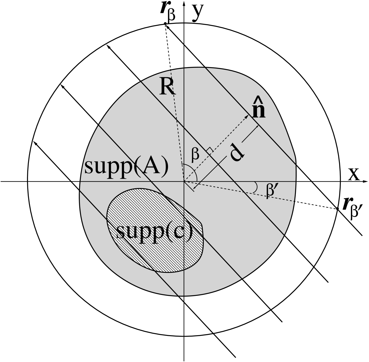
Figure 1: Schematic of the 2D circular measurement geometry employed in the heuristic analysis of Sub-Problem #2 described in Sec. IV. The coordinates $\mathbf{r}_{\beta}$ and $\mathbf{r}_{\beta}^{\prime}$ denote the transducer locations that correspond to the intersection points of the line $\mathbf{r}\cdot\hat{n}=d$ with the measurement circle. In this example, $\text{supp}(c)\subseteq\text{supp}(A)$.

Two cases will be considered that reveal the impact of the relative extents of $\text{supp}(A)$ and $\text{supp}(c)$ on the ability of the oracle to reconstruct $s(\mathbf{r})$, or equivalently, $c(\mathbf{r})$, given $A(\mathbf{r})$. The first case corresponds to the situation where $\text{supp}(c)\subseteq\text{supp}(A)$, as depicted in Fig.  1. In this case, for example, $\text{supp}(A)$ could correspond to the area occupied by a soft tissue structure in which the SOS is approximately the same as the background SOS and $\text{supp}(c)$ would correspond to a region within the tissue possessing a different SOS. It can be verified readily that for every $\mathbf{r}\in\text{supp}(c)$, a collection of $\mathbf{r}_{s}\in\text{supp}(A)$ exists such that values of the data function that specify the line integrals along all paths $L(\mathbf{r}_{\beta}^{\prime},\mathbf{r}_{\beta})$ that intersect $\mathbf{r}$ are accessible to the oracle. Stated otherwise, in this case, all projection data that are needed to uniquely invert the 2D Radon transform [34] in Eq. (17) are accessible and therefore $s(\mathbf{r})$ or, equivalently, $c(\mathbf{r})$ can be exactly determined in a mathematical sense.

In fact, the requirement $\text{supp}(c)\subseteq\text{supp}(A)$ can be relaxed to $\text{supp}(c)$ being enclosed by $\text{supp}(A)$, as shown in Fig. 2(a). This is because we only require $\mathbf{r}_{s}\in\partial\,\text{supp}(A)$, where $\partial\,\text{supp}(A)$ denotes the boundary of $\text{supp}(A)$, to determine the complete set of projection data as described above.

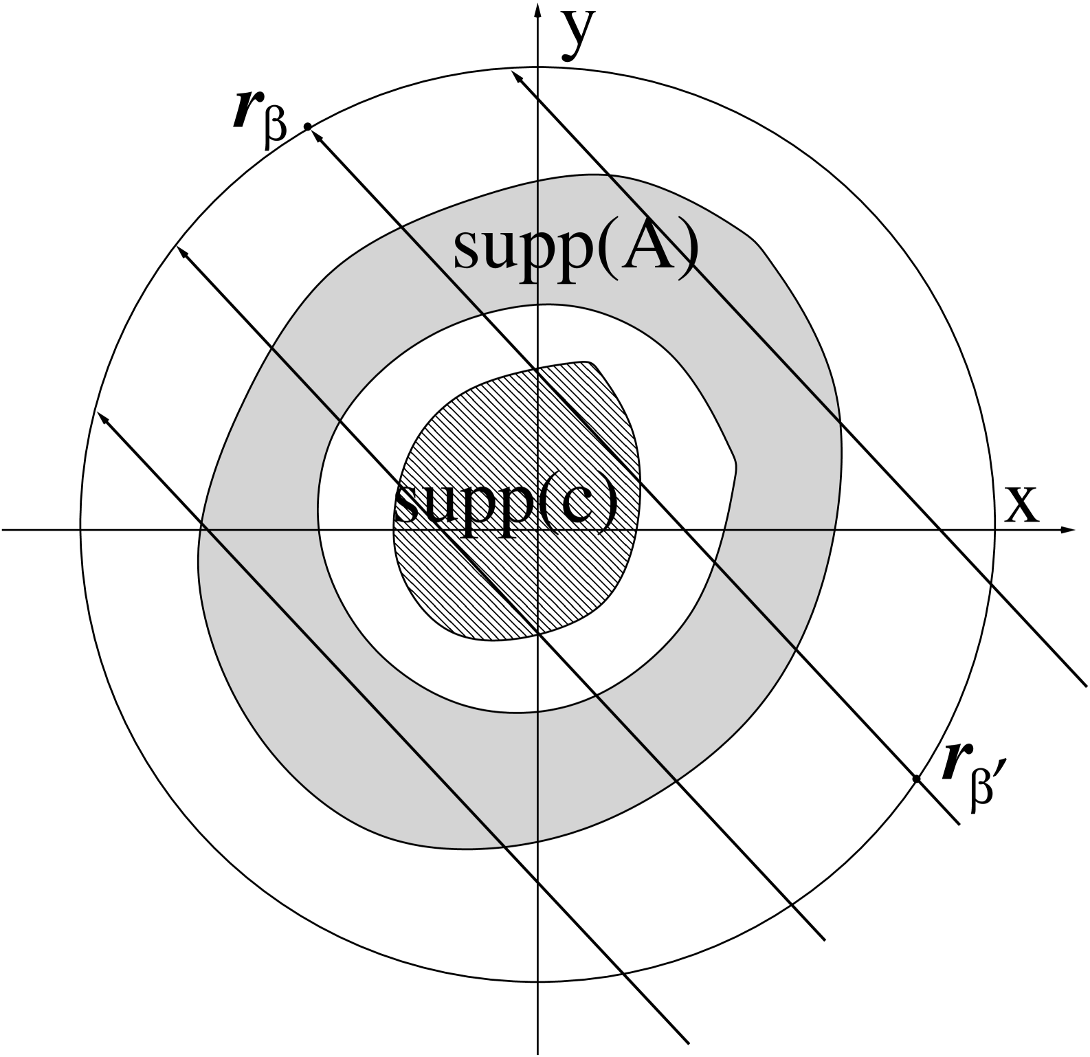
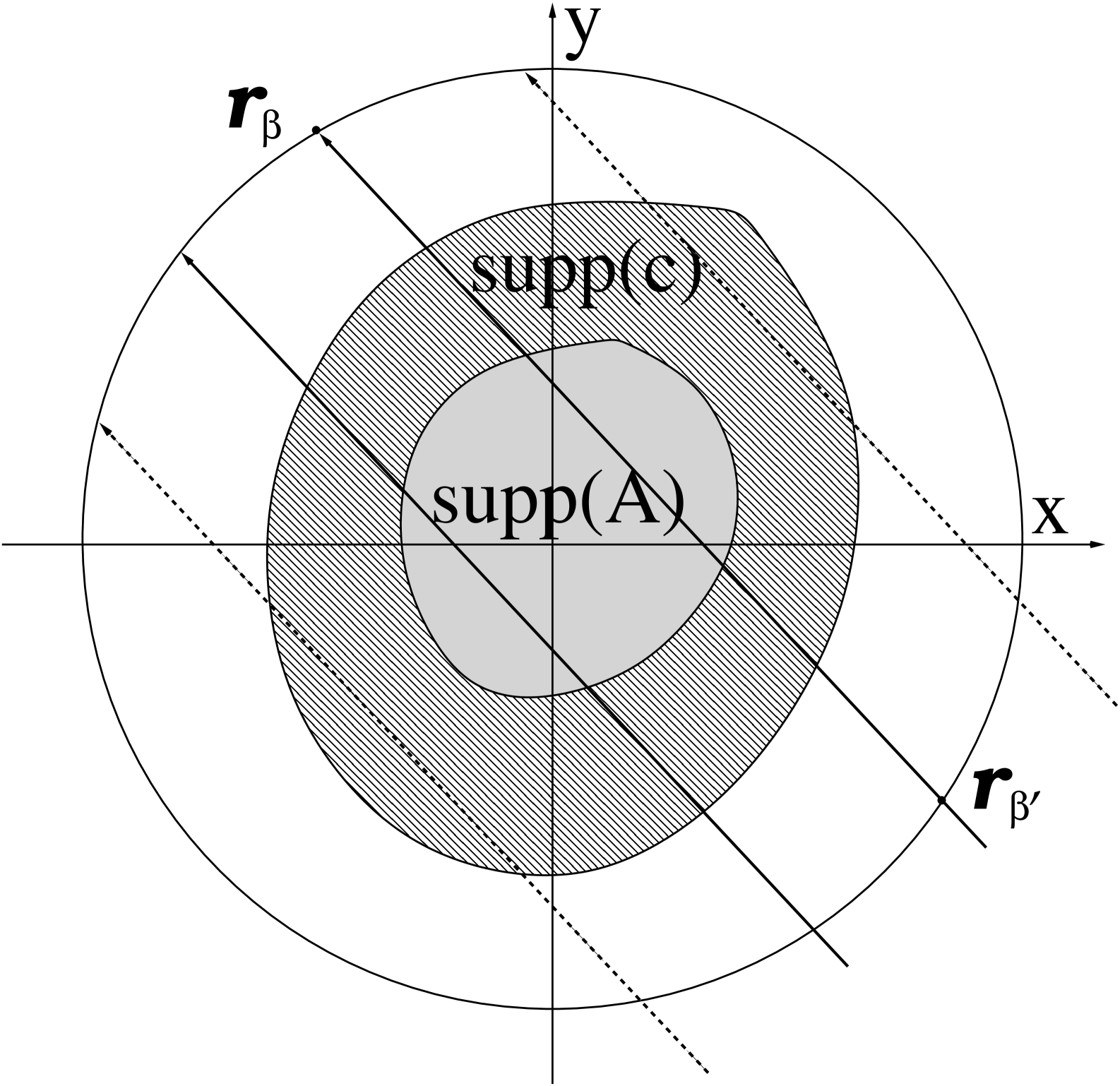
Figure 2: Two cases addressed in the heuristic analysis of Sub-Problem #2 described in Sec. IV: (a) Case where $\text{supp}(c)$ is enclosed by $\text{supp}(A)$; and (b) Case where $\text{supp}(c)$ is not enclosed by $\text{supp}(A)$. In (b), certain line integral data for the slowness distribution in a subset of $\text{supp}(c)$ are not measured, as indicated by the dashed lines through the regions covered by lines.

The second case corresponds to the situation where $\text{supp}(c)$ is not enclosed by $\text{supp}(A)$, as shown in Fig. 2(b). In this case, it can be verified that the complete data function cannot be determined, indicating that the values of all line integrals through $s(\mathbf{r})$ are not accessible as depicted in Fig. 2(b). That example is analogous to the interior problem in X-ray CT, which possesses no unique solution [34].

These observations are summarized as follows.

Support conjecture:: When geometrical acoustics is valid, Sub-Problem #2 cannot be accurately solved when $\text{supp}(c)$ is not enclosed by $\text{supp}(A)$.

V Computer-Simulation Studies

A general description of the computer-simulation methodologies is described below. Although the optimization approach to JR described above is based on the 3D wave equation, 3D JR remains computationally intensive. For computational convenience, the 2D formulation is investigated in this work. The specific numerical experiments designed to investigate the numerical properties of the JR problem are described subsequently in Sec. VI.

V-A Simulation of idealized PA measurement data

Numerical phantoms were utilized to represent $A(\mathbf{r})$ and $c(\mathbf{r})$, which were described by Eqs. (8) and (9). These phantoms, denoted by $\mathbf{A}$ and $\mathbf{c}$, contained $512\times 512$ pixels with a pitch of $0.25$ mm. (i.e., $N=512^{2}$ in Eqs. (8) and (9).) For a given $\mathbf{A}$ and $\mathbf{c}$, the lossless PA wave equation was solved by use of the MATLAB k-Wave toolbox [35] to produce simulated PA signals at each transducer location. Each PA signal contained 6000 temporal samples recorded with a time step $\Delta t=50$ ns. The measurement geometry consisted of 800 transducers that were evenly distributed on the perimeter of a square with a side length of 100 mm. The object was contained within this region. Note that, unless stated otherwise, the generation of the simulated PA measurement data in this way avoided an ‘inverse crime’, due to a different choice of discretization parameters from those employed by the reconstruction algorithm as described below.

V-B Simulation of non-idealized PA measurement data

To investigate the properties of JR under more realistic conditions, additional PA data sets were simulated that considered certain physical factors. Measurement noise was modeled by adding 3% (with respect to the maximum value of the noiseless data) white Gaussian noise (AWGN) to the simulated PA data. Additional factors considered included acoustic attenuation, the effect of the electrical and spatial impulse responses of the transducers. Specific details are provided in Sec. VI-D.

V-C Implementation details for image reconstruction

The implementations of the two image reconstruction sub-problems in Algorithm 1 are described below. The function ‘$\rm{F_{c}}$’ that computes the solution of (15) was implemented based on the MATLAB k-Wave toolbox [35]. Specifically, the wave equation (1) and the adjoint wave equation (4) were solved numerically by use of the k-space pseudospectral method. The computed PA wavefield and the adjoint wavefield were employed to compute the gradient of the objective function in (15) (see Appendix). The gradient was subsequently utilized by the limited-memory BFGS (L-BFGS) algorithm to solve (15) [36, 37, 38]. The implementation of the function ‘$\rm{F_{A}}$’ that solves (14) can be found in [16]. In this study, a total variation (TV) penalty was adopted. The ‘Dist’ function measured the difference in terms of root mean squared error (RMSE), and the convergence tolerances $\epsilon_{A}$ and $\epsilon_{c}$ were empirically chosen to have a value of $10^{-2}$ throughout the studies. In all studies, the initial estimates of $\mathbf{A}$ and $\mathbf{c}$ were set to be $\mathbf{A}^{(0)}=0$ and $\mathbf{c}^{(0)}=1480$ m/s, which is the background SOS. Both $\mathbf{A}$ and $\mathbf{c}$ were reconstructed on a uniform grid of $256\times 256$ pixels with a pitch of 0.5 mm.

All simulations were computed in the MATLAB environment on a workstation that contained dual hexa-core Intel(R) Xeon(R) E5645 CPUs and an NVIDIA Tesla C2075 graphics processing unit (GPU). The GPU was equipped with 448 1.15 GHz CUDA cores and 5 GB global memory. The Jacket toolbox [39] was employed to accelerate the computation of (1) and (4) on the GPU.

VI Numerical investigations and analyses

VI-A Topology of the JR cost function in Eq. (13)

The effectiveness of the optimization-based approach to JR depends on the topology of the cost function that is minimized in Eq. (13). In these studies, only the data fidelity term was considered ($\lambda_{1}=\lambda_{2}=0$). If the cost function is not convex or quasi-convex, a global minimum (i.e., an accurate JR solution) may not be returned by the optimization algorithm when the initial estimate is not close enough to the global minimizer. Moreover, when the cost function is not strictly convex, there is no guarantee that the solution is unique. In this section, a low-dimensional stylized example is considered to yield insights into the general characteristics of the cost function topology.

The numerical phantoms shown in Fig. 3 were employed to represent $\mathbf{A}$ and $\mathbf{c}$. To establish a low-dimensional representation of these phantoms, a discretization scheme that differed from Eqs. (8) and (9) was employed (in this study only). Namely, $\mathbf{A}$ was described as $\mathbf{A}=[A_{s},A_{b}]$ where $A_{s}$ represented the value within the uniform disk and $A_{b}$ is the known (assumed to be zero) background value. Similarly, $\mathbf{c}$ was described as $\mathbf{c}=[c_{s},c_{b}]$ where $c_{s}$ represented the value of the uniform annulus and $c_{b}$ is the fixed background value outside of the annulus. For each $(A_{s},c_{s})$ pair, simulated PA data $\hat{\mathbf{p}}$ were computed. Subsequently, the value of $\|\mathbf{H}(\mathbf{c})\mathbf{A}-\hat{\mathbf{p}}\|^{2}$ was computed and plotted as a function of the scale factors of $A_{s}$ and $c_{s}$.

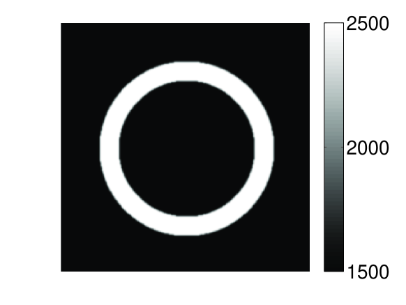
Figure 3: Subfigures (a) and (b) display the numerical phantoms that specified $\mathbf{A}$ and $\mathbf{c}$ that were employed to investigate the JR cost function topology in Sec. VI-A.

Figure 4(a) displays a surface plot of the data fidelity term $\|\mathbf{H}(\mathbf{c})\mathbf{A}-\hat{\mathbf{p}}\|^{2}$ as a function of the scale factors of $A_{s}$ and $c_{s}$, while profiles corresponding to $A_{s}=1$ are shown in subfigure (b). The results show that the data fidelity term is not convex with respect to $\mathbf{c}_{s}$. These results suggest the cost function may also be non-convex with respect to more general and higher-dimensional SOS distributions $\mathbf{c}$.

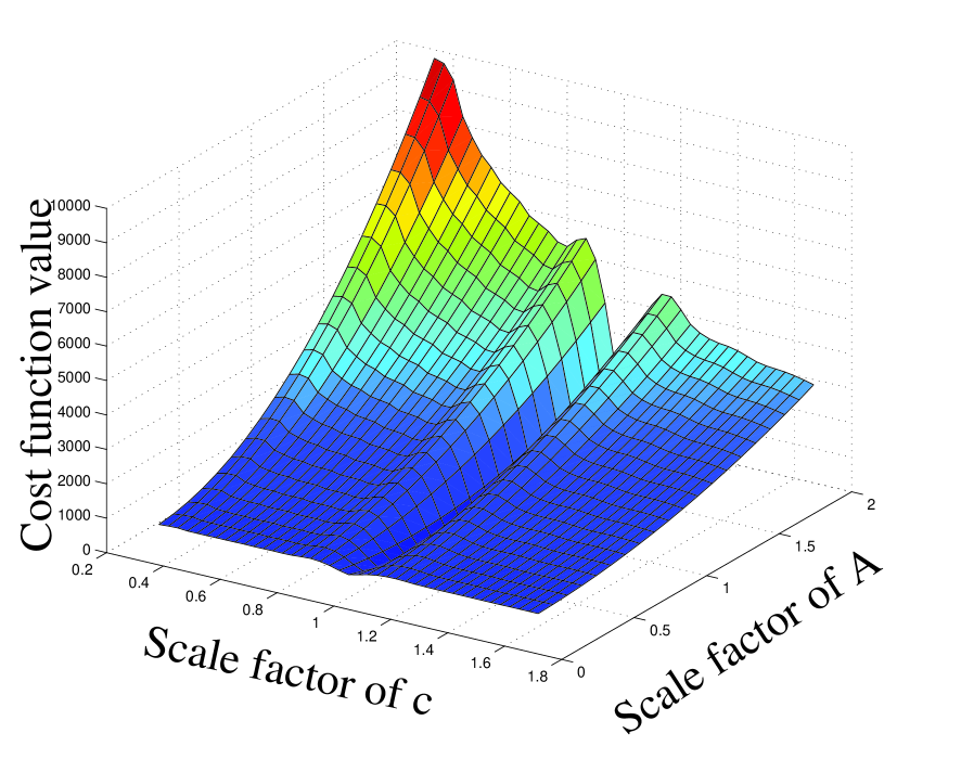
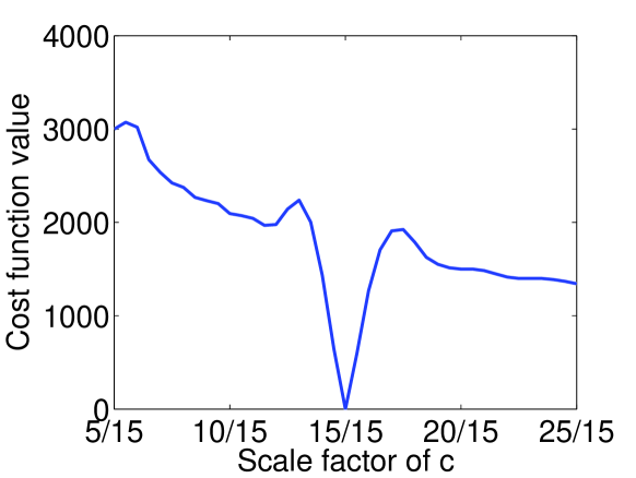
Figure 4: Subfigure (a) displays a surface plot of the data fidelity term in the JR cost function and the corresponding profile corresponding to $A_{s}=1$ is shown in subfigure (b). Details are provided in Sec. VI-A.

To investigate how the spatial structure of $\mathbf{A}$ can influence the topology of the cost function, the above procedure was repeated when the radius of the disk in $\mathbf{A}$ was varied. Profiles of the normalized data fidelity term corresponding to $A_{s}=1$ are displayed in Fig. 5(a). These data reveal that the ‘valley’ containing the global minimum of the cost function widens as the radius of the disk heterogeneity in $\mathbf{A}$ increases. This can be seen more clearly in the plots of the width of the valley versus the disk radius that are shown in Fig. 5(b). This observation suggests that the quality of the initial estimate for $\mathbf{c}$ can be relaxed when the radius of the support of $\mathbf{A}(\mathbf{r})$ increases.

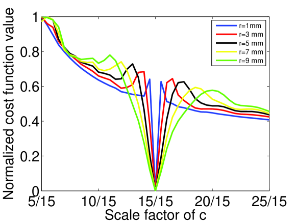
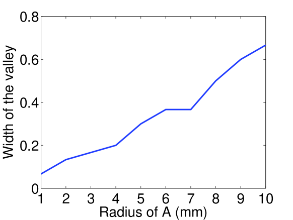
Figure 5: Profiles of the normalized data fidelity term corresponding to $A_{s}=1$ for different radii of the disk phantom that specified $\mathbf{A}$ are displayed in subfigure (a). Subfigure (b) displays a plot of the width of the valleys in (a) versus the disk radius.

In summary, these results establish that, for a fixed $\mathbf{A}$, the JR cost function is generally non-convex with respect to $\mathbf{c}$. Accordingly, Sub-Problem #2 is generally a non-convex problem. Sub-Problem #1 is convex if the penalty is convex. The overall non-convexity of the JR problem indicates that accurate initial estimates of $\mathbf{c}$ will generally be necessary to avoid local minima that represent inaccurate solutions. Additionally, the non-convexity of the problem suggests that uniqueness of the solution is not guaranteed.

VI-B Numerical investigations of Sub-Problem #2

As described above, Sub-Problem #2 corresponds to a non-convex optimization problem that can be difficult to solve in practice. Accordingly, errors that arise when solving Sub-Problem #2 can accumulate in Algorithm 1 and hinder the ability to perform accurate JR. Below, numerical experiments are reported that reveal insights into some mathematical properties of $A(\mathbf{r})$ and $c(\mathbf{r})$ that influence the ability to accurately solve Sub-Problem #2.

VI-B1 Effect of spatial supports of $A(\mathbf{r})$ and $c(\mathbf{r})$

Studies were conducted to investigate the extent to which the support conjecture, provided in Sec. IV, influences the ability to accurately solve Sub-Problem #2, and hence perform JR, by use of perfect measurements. The numerical phantom employed to represent the SOS distribution, $\mathbf{c}$, is shown in Fig. 6. The SOS values were representative of human breast tissues. We first considered two choices for $\mathbf{A}$, shown in Figs.  7(a) and 7(d), which were designed to satisfy the support conjecture ($\text{supp}(c)$ is enclosed by $\text{supp}(A)$). For each choice of $\mathbf{A}$, a corresponding estimate of $\mathbf{c}$ was estimated by solving Sub-Problem #2 from noiseless simulated PACT measurements. The value of the regularization parameter $\lambda_{c}$ in Eq. (15) was zero. The reconstructed estimates of $\mathbf{c}$ corresponding to the two choices of $\mathbf{A}$ are shown in Figs. 7(b) and 7(c). The corresponding profiles extracted from the central rows of the reconstructed estimates are displayed in Figs. 7(c) and 7(f), respectively. These results reveal that it is possible to reconstruct accurate estimates of $\mathbf{c}$ from perfect PACT measurements via Sub-Problem #2 when the specified $\mathbf{A}$ satisfies the support conjecture. The effects of noise and other measurement errors are addressed later.

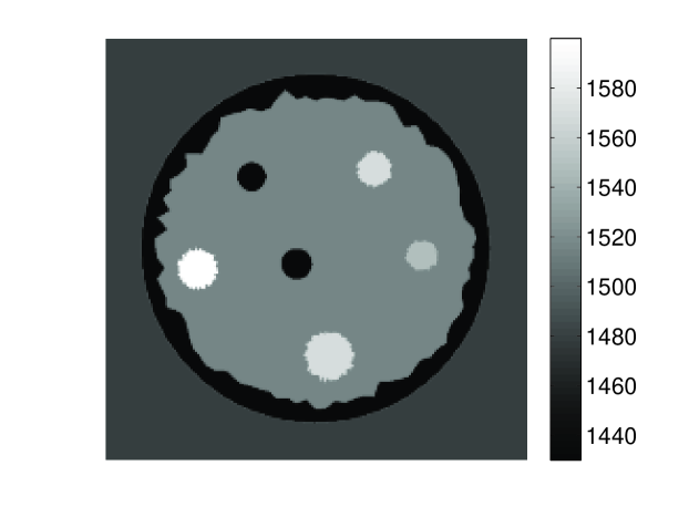
Figure 6: The numerical SOS phantom described in Sec. VI-B that was utilized in the investigations of Sub-Problem #2.

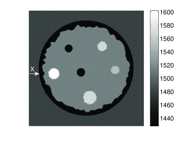
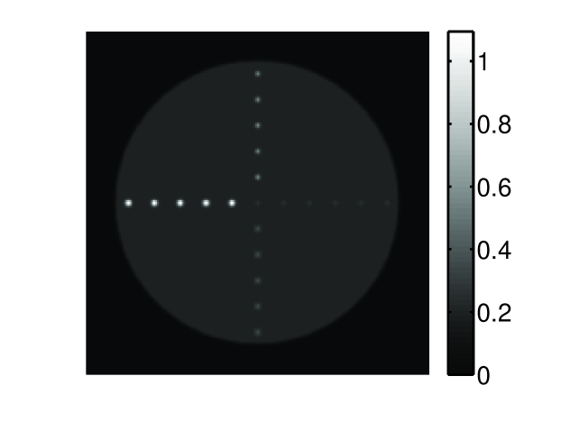
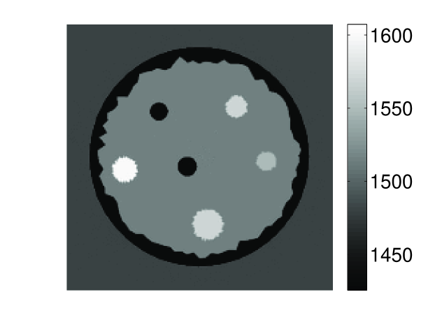
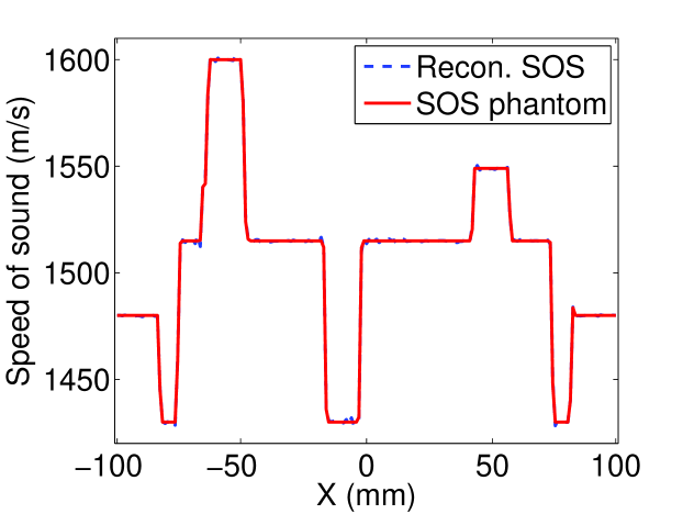
Figure 7: Numerical investigations of Sub-Problem #2 - Spatial support effects: Two different phantoms $\mathbf{A}$ that satisfy the support conjecture are shown in subfigures (a) and (d). The estimates of $\mathbf{c}$ obtained by solving Sub-Problem #2 by use of noiseless data and the corresponding $\mathbf{A}$ are shown in subfigures (b) and (e). Image profiles through the estimates of $\mathbf{c}$ are shown in subfigures (c) and (f).

We next considered the four choices for $\mathbf{A}$, shown in the left column of Fig. 8 (Figs. 8(a), (d), (g), and (j)), which, roughly speaking, were designed to violate the support conjecture to different extents. As above, corresponding unregularized estimates of $\mathbf{c}$ were estimated by solving Sub-Problem #2 from noiseless simulated PACT measurements. The reconstructed estimates of $\mathbf{c}$ corresponding to the different choices of $\mathbf{A}$ are shown in the middle column of Fig. 8. The corresponding profiles extracted from the central rows of the reconstructed estimates are displayed in the right column. Figures 8(b) and (e) reveal that, despite that the violation of the support conjecture, accurate estimates of $\mathbf{c}$ could still be reconstructed. Figures 8(h) and (k) demonstrate that the accuracy of the reconstructed estimate of $\mathbf{c}$ degrades as the size of the support of $A(\mathbf{r})$ is reduced.

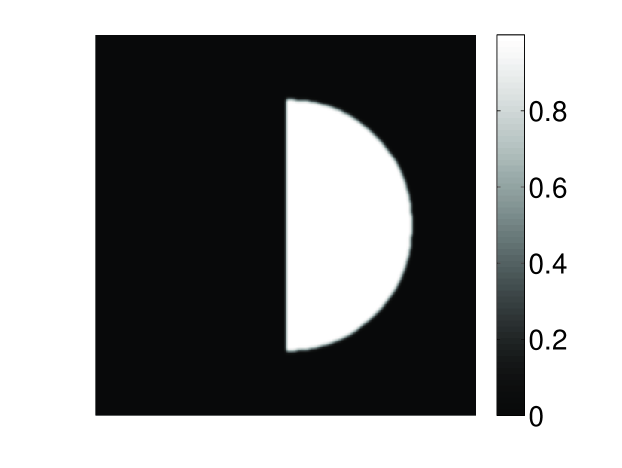
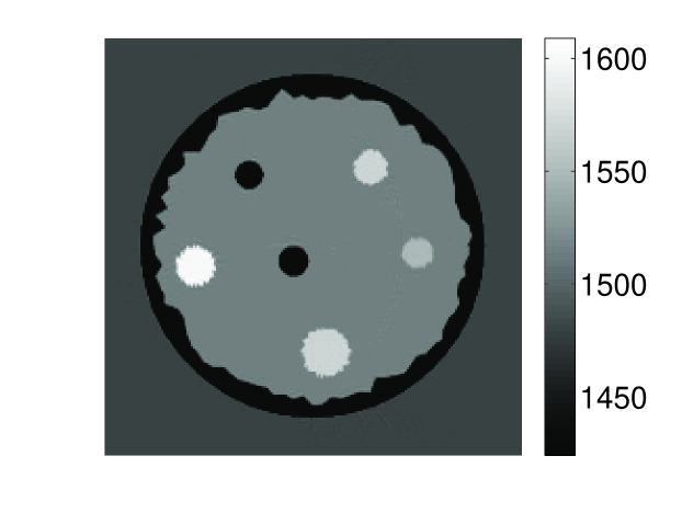
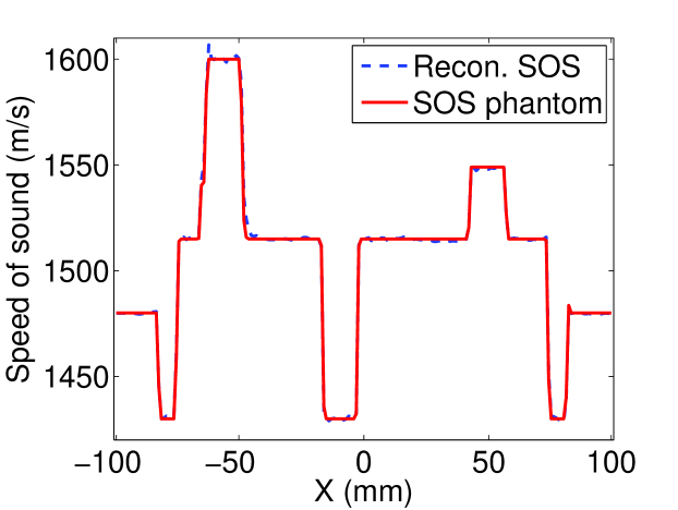
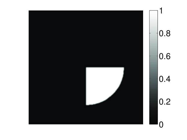
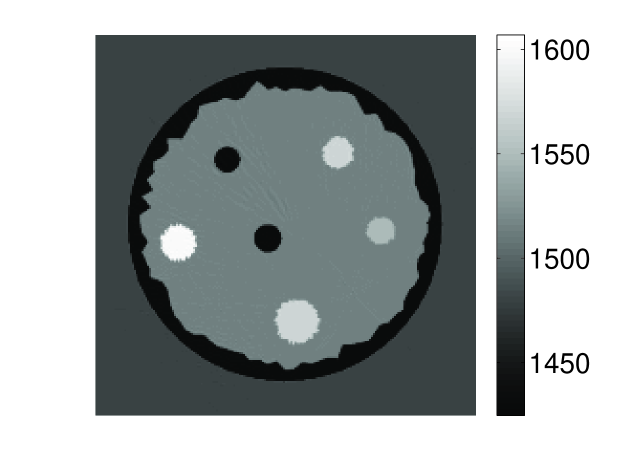
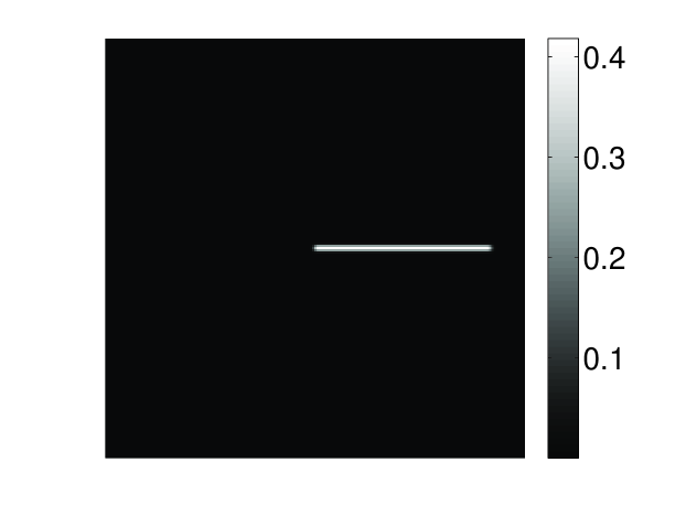
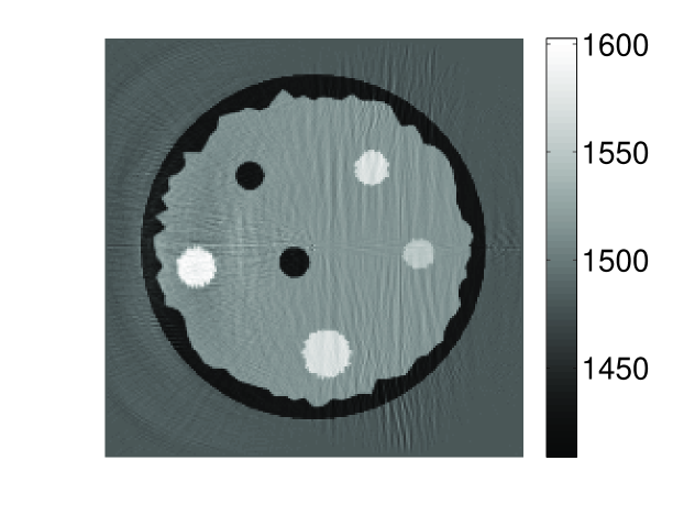
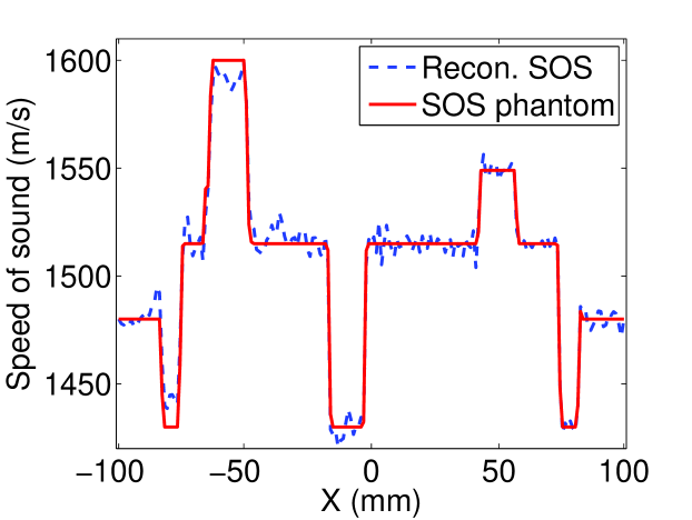
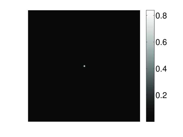
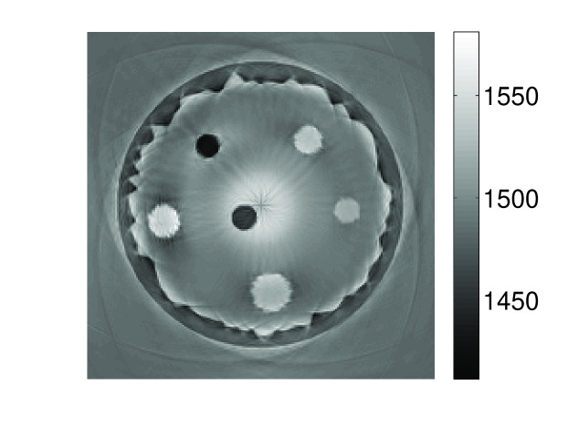
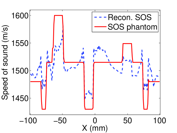
Figure 8: Numerical investigations of Sub-Problem #2 - Spatial support effects: Four different phantoms $\mathbf{A}$ that violated the support conjecture are shown in subfigures (a), (d), (g), and (j). The estimates of $\mathbf{c}$ obtained by solving Sub-Problem #2 by use of noiseless data and the corresponding $\mathbf{A}$ are shown in subfigures (b), (e), (h), and (k). Image profiles through the estimates of $\mathbf{c}$ are shown in subfigures (c), (f), (i), and (l).

In summary, these observations reveal that, in general, the support conjecture does not need to be satisfied in order to achieve accurate reconstruction of $\mathbf{c}$ for an exactly known $\mathbf{A}$ and perfect measurement data. This may be explained by the fact that the support conjecture was established by use of geometrical acoustics that represents a simplification of the complicated acoustic wave propagation in both our simulations or in practice. However, in the cases where the support conjecture was satisfied, $\mathbf{c}$ was accurately estimated. Moreover, the simulation results indicate that the extent to which the supports of $A(\mathbf{r})$ and $c(\mathbf{r})$ overlap does affect the ability to accurately solve Sub-Problem #2, and hence the JR problem.

VI-B2 Effect of relative spatial bandwidths of $A(\mathbf{r})$ and $c(\mathbf{r})$

Studies were conducted to investigate the extent to which the relative spatial bandwidths of $A(\mathbf{r})$ and $c(\mathbf{r})$ influence the ability to accurately solve Sub-Problem #2 by use of perfect measurements. Figure 9 shows the numerical phantoms for $\mathbf{A}$ and $\mathbf{c}$. To exclude the effects related to the supports of $A(\mathbf{r})$ and $c(\mathbf{r})$, the phantoms were designed to satisfy the support conjecture. The spatial structures of the original phantoms in Fig. 9 are identical, indicating that their spatial frequency bandwidths are identical. The phantom depicting $\mathbf{A}$ was subsequently convolved with different Gaussian kernels to generate additional phantoms that possessed different spatial frequency bandwidths. The full width at half maximum (FWHM) of the blurring kernel was employed as a summary measure of the relative spatial bandwidths of the smoothed phantoms. Sub-Problem #2 was subsequently solved with $\lambda_{c}=0$ by use of both perfect and noisy simulated measurement data for each of the smoothed versions of $\mathbf{A}$.

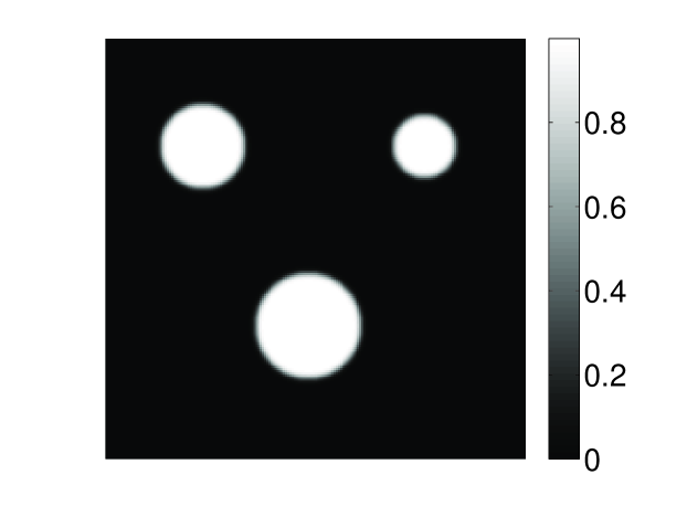
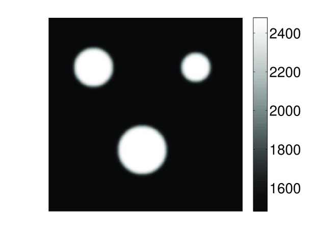
Figure 9: The numerical phantoms representing (a) $\mathbf{A}$ and (b) $\mathbf{c}$ that are described in Sec. VI-B2.

The reconstructed estimates of $\mathbf{c}$ are shown in Fig. 10. From top to bottom, the results correspond to relative bandwidth ratios (of $\mathbf{A}$ to $\mathbf{c}$) of 0.25, 0.44, and 1.0, respectively. Figures 10(a), (e), and (i) correspond to images reconstructed from perfect measurement data and the associated image profiles are displayed in Figs.  10(b), (f), and (j). Figures 10(c), (g), and (k) correspond to images reconstructed from noisy measurement data and the associated image profiles are displayed in Figs.  10(d), (h), and (l). The RMSE of the reconstructed $\mathbf{c}$ with respect to the relative bandwidth ratio of $\mathbf{A}$ to $\mathbf{c}$ for both noiseless and noisy cases is displayed in Fig. 11.

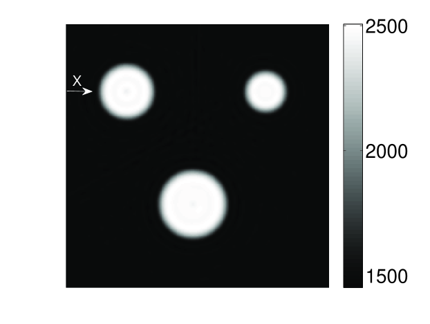
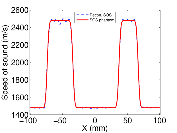
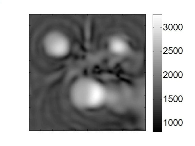
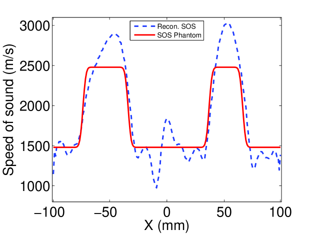
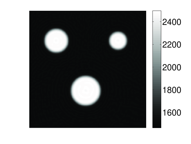
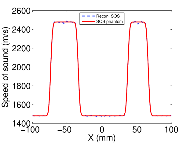
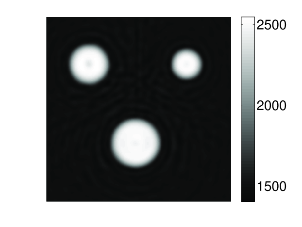
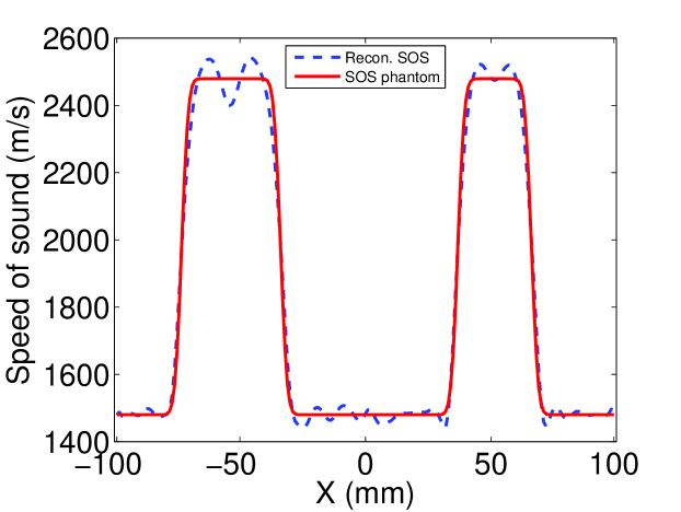
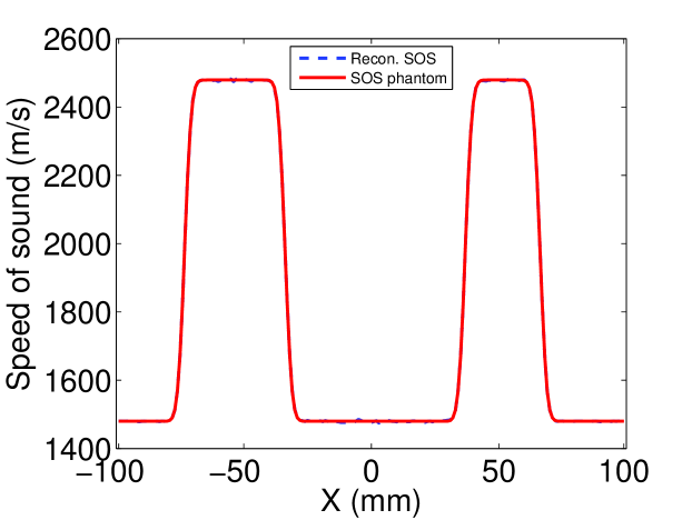
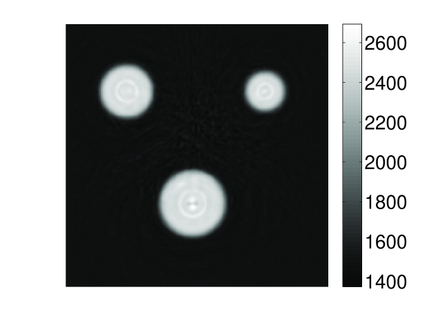
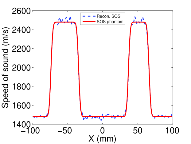
Figure 10: Numerical investigations of Sub-Problem #2 - Spatial bandwidth effects: As described in Sec. VI-B2, unregularized estimates of $\mathbf{c}$ were reconstructed from noiseless and noisy data and a series of $\mathbf{A}$ that had different spatial bandwidths relative to that of the sought-after $\mathbf{c}$. From the top to the bottom rows, the results correspond to relative bandwidths of $\mathbf{A}$ to $\mathbf{c}$ of 0.25, 0.44, and 1.0, respectively. Subfigures (a), (e), and (i) correspond to images reconstructed from perfect measurement data and the associated image profiles are displayed in subfigures (b), (f), and (j). Subfigures (c), (g), and (k) correspond to images reconstructed from noisy measurement data and the associated image profiles are displayed in subfigures (d), (h), and (l).

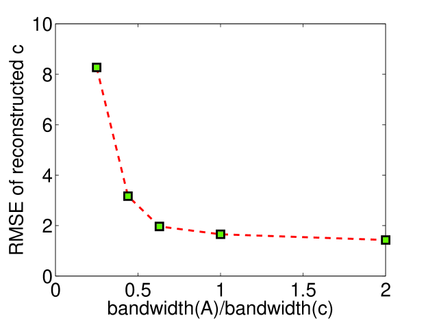
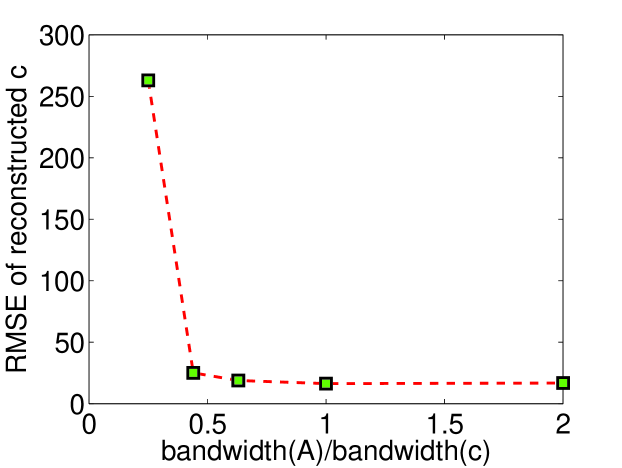
Figure 11: Numerical investigations of Sub-Problem #2 - Spatial bandwidth effects: Plots of RMSE of the estimated $\mathbf{c}$ as a function of the bandwidth ratio of $\mathbf{A}$ to $\mathbf{c}$. Subfigures (a) and (b) correspond to the noiseless and noisy results, repectively.

These results reveal that the relative spatial frequency bandwidths of $A(\mathbf{r})$ and $c(\mathbf{r})$ affect the numerical stability of Sub-Problem #2 and, hence, that of the JR problem. The accuracy of the reconstructed $\mathbf{c}$ in the present of measurement noise for a specified $\mathbf{A}$ was observed to be influenced strongly by the relative spatial bandwidths of $\mathbf{A}$ and $\mathbf{c}$. Specifically, in order to accurately reconstruct $\mathbf{c}$ in the presence of noise, the presented results suggest that the spatial frequency bandwidth of $A(\mathbf{r})$ should be comparable to or larger than the spatial frequency bandwidth of $c(\mathbf{r})$. We will refer to this as the k-space conjecture hereafter.

VI-B3 Effect of perturbations of $A(\mathbf{r})$

In the studies described above, perfect knowledge of $\mathbf{A}$ was assumed. Below, a numerical experiment is described that provides insights into how small perturbations in the assumed $\mathbf{A}$ affects the accuracy of the reconstructed $\mathbf{c}$ obtained by solving Sub-Problem #2.

Figures 12(a) and (c) display two similar numerical phantoms depicting $\mathbf{A}$. The RMSE between these phantoms is $0.004$. Perfect PACT measurements were simulated for each of the two $\mathbf{A}$, for a given $\mathbf{c}$ (not shown). Figures 12(b) and (d) display the reconstructed estimates of $\mathbf{c}$ when the $\mathbf{A}$ specified in Fig. 12(a) and (c) was assumed, respectively. These results demonstrate that the problem of reconstructing $\mathbf{c}$ for a given $\mathbf{A}$ is ill-conditioned in the sense that small changes in $\mathbf{A}$ can produce significant changes in the reconstructed estimate of $\mathbf{c}$. This observation is consistent with the theoretical results in [30].

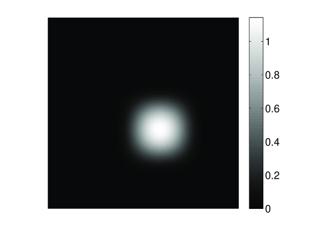
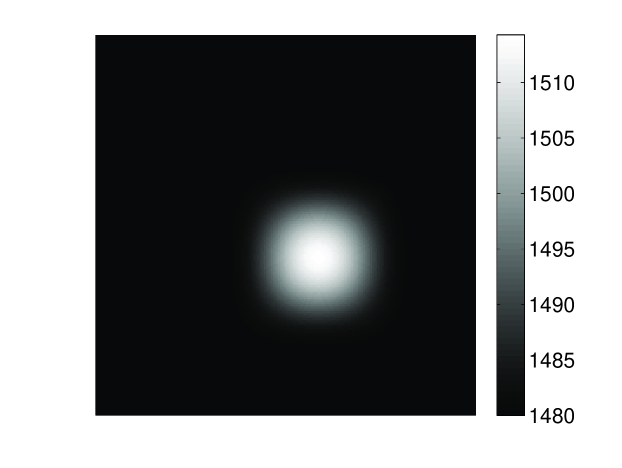
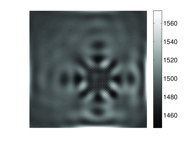
Figure 12: Numerical investigations of Sub-Problem #2 - Effect of perturbation of $\mathbf{A}$: Two numerical phantoms representing $\mathbf{A}$ are shown in subfigures (a) and (c). As described in Sec. VI-B3, these two phantoms are very similar, with a RMSE between them of only $0.004$. Unregularized estimates of $\mathbf{c}$ reconstructed by use of noiseless simulated measurement data and the $\mathbf{A}$ specified in (a) and (c) are shown in subfigures (b) and (d), respectively. Although the phantoms depicting $\mathbf{A}$ are very similar, the reconstructed estimates of $\mathbf{c}$ are not.

It is interesting to note that the ($\mathbf{A}$, $\mathbf{c}$) pair in the top row of Fig. 12 produces nearly identical PA data, at all transducer locations, to that produced by the ($\mathbf{A}$, $\mathbf{c}$) pair in the bottom row. The simulated noiseless pressure data at an arbitrary transducer location produced by the two ($\mathbf{A}$, $\mathbf{c}$) pairs is shown in Fig. 13, where the pressure signals are observed to overlap almost completely. The RMSE between the two sets of PA data was $\text{RMSE}=3.2\times 10^{-4}$. These results suggest that the solutions of the JR problem in PACT may not be unique. Consequently, it indicates that accurate JR of $\mathbf{A}$ and $\mathbf{c}$, in general, may not be possible.

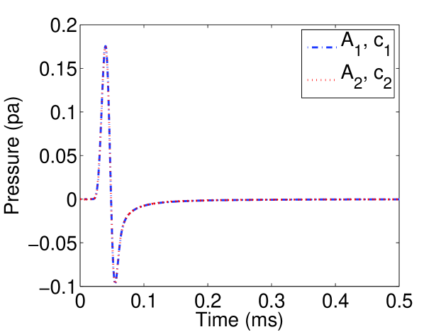
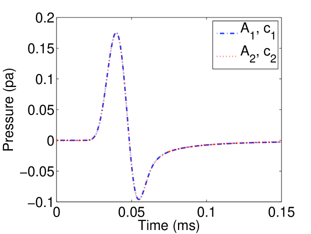
Figure 13: Numerical evidence of non-uniqueness of the JR problem: Simulated PA measurement data were computed from the $(\mathbf{A},\mathbf{c})$ pairs shown in Figs. 12(a) and (b) and Figs. 12(c) and (d). The two pressure profiles corresponding to an arbitrary transducer location are superimposed in subfigure (a). Subfigure (b) displays a zoomed-in version of subfigure (a). Similar agreement between the profiles was observed at all transducer locations.

VI-C Feasibility of JR with idealized data

The numerical instability of Sub-Problem #2, as examined in the previous section, implies that the solution to the JR problem is also numerically unstable. This was confirmed by computing solutions to the JR problem from perfect measurement data. The data were perfect in the sense that they did not contain measurement noise. Moreover, ‘inverse crime’ was committed in which the same forward model and discretization parameters (pixel size $=0.5$ mm) were employed to produce the simulation data and to conduct image reconstruction. These data were produced by use of the phantoms shown in Fig.  9, which satisfied both the support and the k-space conjectures. Unregularized JR was performed by use of Algorithm 1 with $\lambda_{A}=\lambda_{c}=0$ and the results are displayed in the top row of Fig. 14. Despite the use of perfect measurement data and a favorable choice of $\mathbf{A}$ and $\mathbf{c}$, neither $\mathbf{A}$ nor $\mathbf{c}$ could be accurately reconstructed.

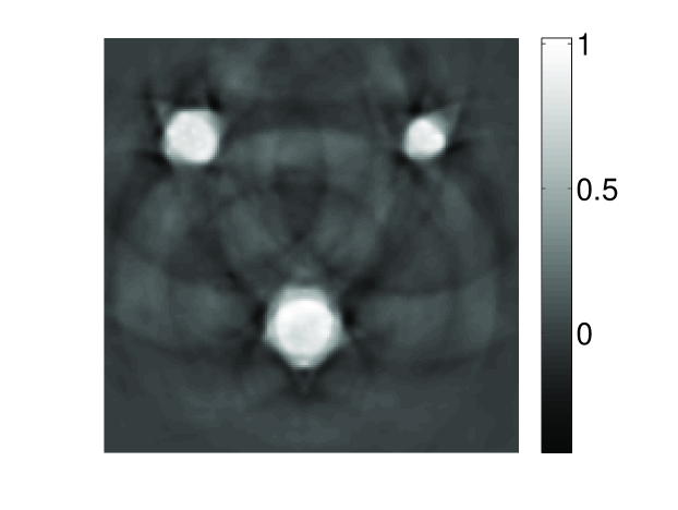
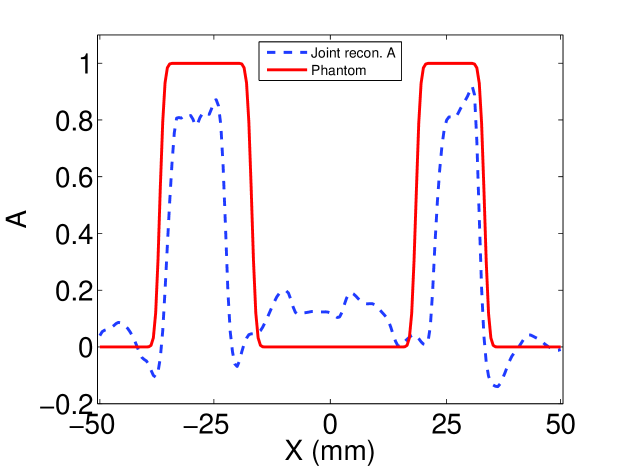
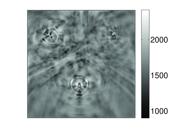
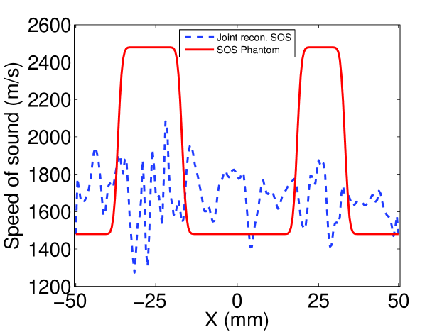
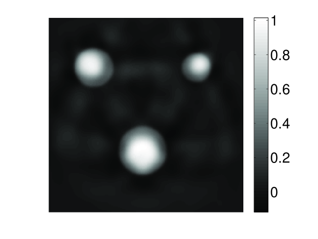
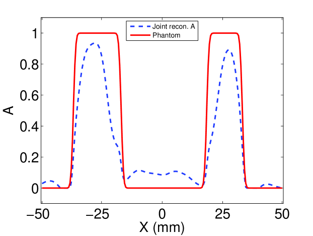
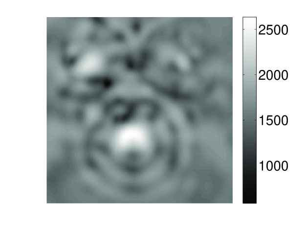
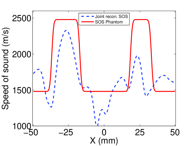
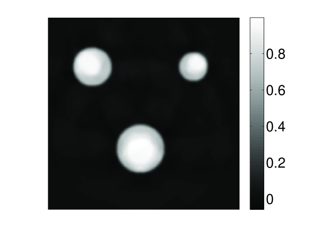
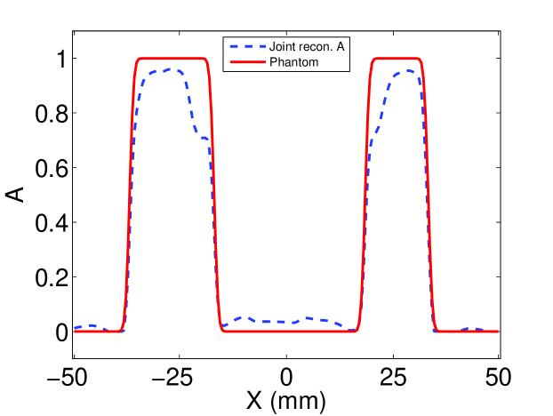
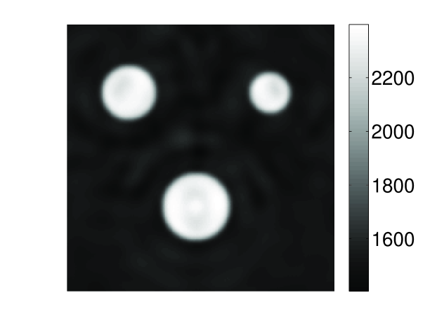
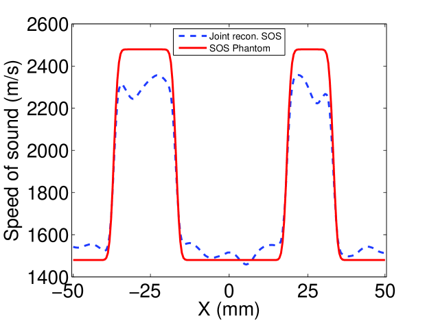
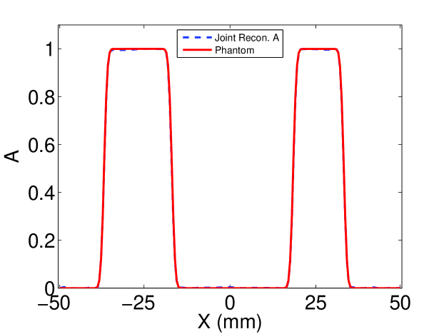
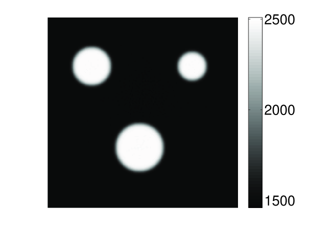
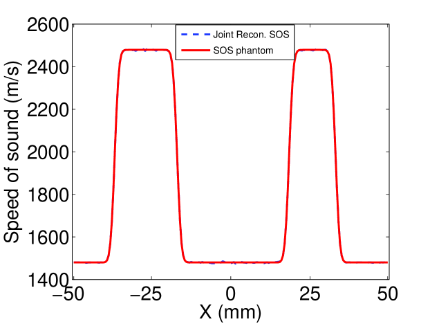
Figure 14: Images obtained via JR from noiseless PA measurements: The first and third columns display the estimates of $\mathbf{A}$ and $\mathbf{c}$, and the corresponding image profiles are displayed in the second and fourth columns, respectively. Each row corresponds to use of different regularization parameters $\lambda_{A}$ and $\lambda_{c}$. From top to bottom, $(\lambda_{A},\lambda_{c})$ are $(0,10^{-5})$, $(10^{-4},10^{-3})$, $(0,10^{-4})$, and $(10^{-3},10^{-2}$), respectively.

Additional studies were conducted in which noiseless measurement data were computed without committing inverse crime. Namely, the pixel size employed to simulate the measurement data was 0.5 times the pixel size employed in the reconstruction algorithm. From these data, regularized estimates of $\mathbf{A}$ and $\mathbf{c}$ were computed. In rows 2-4 of Fig. 14, the corresponding regularization parameters are $\lambda_{A}=\lambda_{c}=10^{-5}$, $10^{-4}$, and $10^{-3}$, respectively. These results demonstrate that the numerical instability of the JR problem can be mitigated by incorporating appropriate regularization. However, the salient observation here is that regularization was required to obtain accurate image estimates, even if no stochastic measurement noise or other significant modeling errors other than discretization effects were introduced.

VI-D Feasibility of JR with imperfect data

VI-D1 Effect of stochastic measurement noise

JR was performed by use of noisy versions of the PA data. The first and second rows of Fig. 15 display the estimates of $\mathbf{A}$ and $\mathbf{c}$, respectively, along with corresponding image profiles. These results were obtained with regularization parameters $\lambda_{A}=10^{-3}$ and $\lambda_{c}=10^{-2}$. There results show that, with appropriate regularization, JR can be robust to the effects of AWGN.

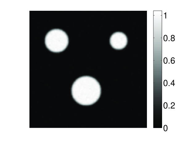
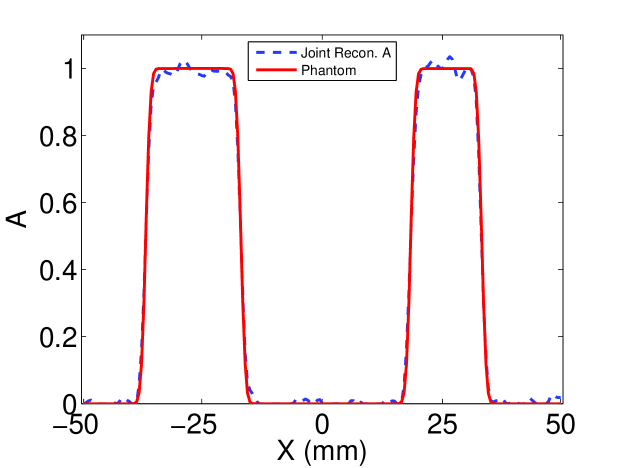
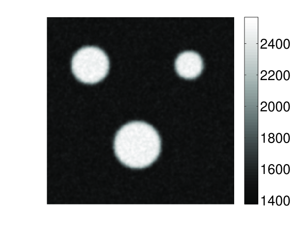
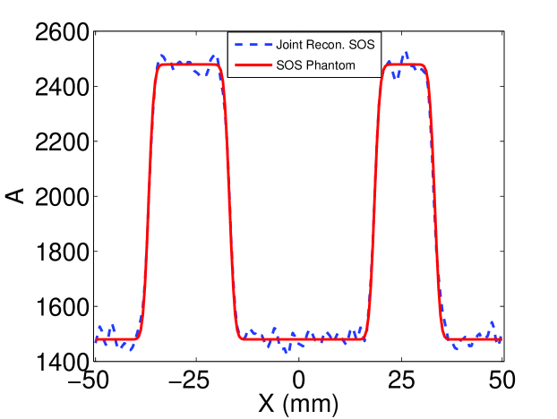
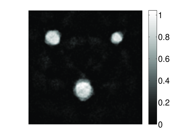
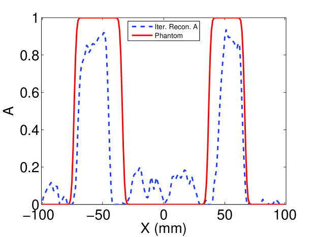
Figure 15: Images obtained via JR from noisy PA measurements: The top and middle rows display the reconstructed estimates of $\mathbf{A}$ and $\mathbf{c}$, respectively, along with the corresponding image profiles. The bottom row displays an estimate of $\mathbf{A}$ reconstructed by a PACT reconstruction method that employed a constant SOS that was manually tuned to minimize RMSE.

To compare with the JR results, $\mathbf{A}$ was also reconstructed by use of a full-wave PACT reconstruction method [16] that neglected acoustic heterogeneity by employing a constant SOS value. This estimate of $\mathbf{A}$ is displayed in the third row of Fig 15. The reconstruction method assumed a constant SOS value of 1600 m/s, which was manually tuned to minimize the RMSE of the reconstructed image. The RMSE of the reconstructed $\mathbf{A}$ by use of the JR method and the PACT method ignoring SOS variations was $0.01$ and $0.21$, respectively. These results confirm that the estimate of $\mathbf{A}$ obtained by performing JR is more accurate than the corresponding estimate reconstructed by use of a PACT method assuming a constant SOS.

VI-D2 Effect of other modeling errors

In practice, besides stochastic measurement noise due to the electronics, other forms of measurement data inconsistency will be present. For example, the imaging model utilized in this work neglects the spatial impulse response (SIR) of the transducers and acoustic attenuation within the object and coupling medium [40, 41, 42, 43, 44, 33]. Additionally, because the pressure data are assumed to represent the measurable quantity, the electrical impulse response (EIR) of the transducer is assumed to be known exactly and the deconvolution process to obtain the pressure data is assumed to be error-free. These assumptions will be violated in a real-world experiment. A study was conducted to demonstrate the performance of JR based on our idealized imaging model in the presence of stochastic measurement noise and these factors that are neglected or only partially compensated for.

The simulated PA data containing the effects of these physical factors was generated as follows.

1. Simulated PA data were generated in a lossy medium. The $\mathbf{A}$ and $\mathbf{c}$ phantoms shown in Fig. 9 were employed. Acoustic attenuation was introduced by use of an acoustic attenuation coefficient $\alpha$ that was described by a frequency power law of the form $\alpha(\mathbf{r},f)=\alpha_{0}(\mathbf{r})f^{y}$ [45]. The frequency-independent attenuation coefficient $\alpha_{0}=10$ dB MHz and the power law exponent $y=2.0$ were employed in the data generation, which correspond to the values of $\alpha_{0}$ and $y$ in human kidneys that have the strongest acoustic attenuation among typical biological tissues [46]. The simulated PA data were contaminated by 3% AWGN.

2. To model the effects of the SIR, the simulated PA data, described above, were computed on a grid with a pitch of 0.1 mm and recorded by 4000 transducers that were evenly distributed on the sides of a square with side length 100 mm. The recorded data from every 20 consecutive transducers were then averaged to emulate the SIR of a 2 mm line transducer. Note that this simplified model of the SIR accounts only for the averaging of the pressure data over the active surface of a transducer [47] and neglects other factors that may contribute to the SIR of a real-world transducer.

3. The simulated PA data containing the acoustic attenuation effects, the SIR effects and measurement noise were convolved with an EIR of an actual transducer [48, 40]. The convolved data were then deconvolved by use of a curvelet deconvolution technique [49]. In the deconvolution, a perturbed EIR was employed that was produced by adding 2% Gaussian noise into the spectrum of the original EIR. Figure 16(a) displays the perturbed and original EIR and Fig.  16(b) displays the deconvolved and true pressure signal for a particular transducer location.

   

   

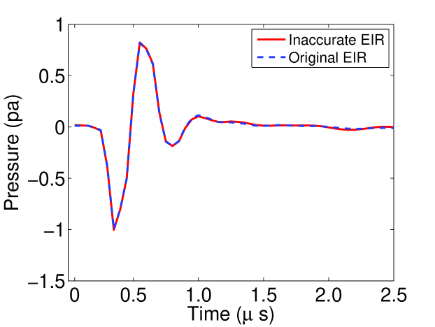
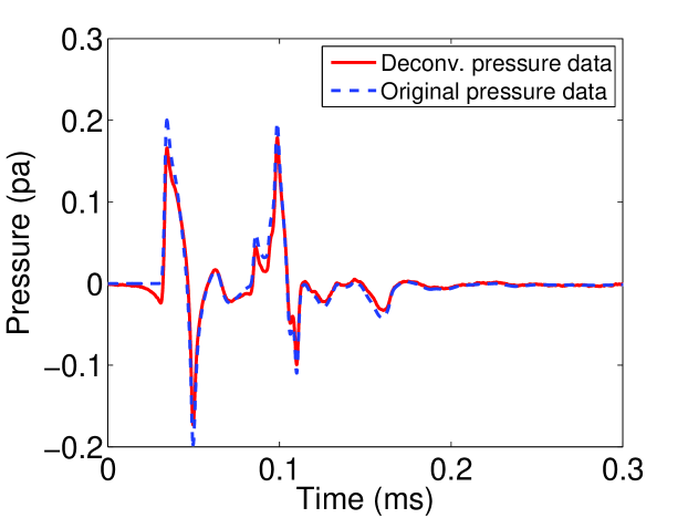
   Figure 16: Panel (a): inaccurate EIR compared to the original EIR. Panel (b): deconvolved pressure data by use of the inaccurate EIR compared to original pressure data.

From these data, JR of $\mathbf{A}$ and $\mathbf{c}$ was performed with regularization parameters $\lambda_{A}=10^{-2}$ and $\lambda_{c}=10^{-1}$. The JR results are displayed in the top and middle rows of Fig. 17. These results suggest that, even with a sufficient $\mathbf{A}$ that satisfies the support and k-space conjectures, accurate JR may not be feasible in practice due to its instability unless model errors are small. However, the jointly reconstructed $\mathbf{A}$ has smaller RMSE = 0.12 compared to the iterative result (the bottom row of Fig. 17) that was reconstructed with constant SOS of 1600 m/s and has RSME = 0.22. This shows that, even though accurate JR may not be feasible in practice, the JR method provides the opportunity to improve the accuracy of the reconstructed $\mathbf{A}$ as compared to the use of a PACT reconstruction method that assumes a constant SOS [50].

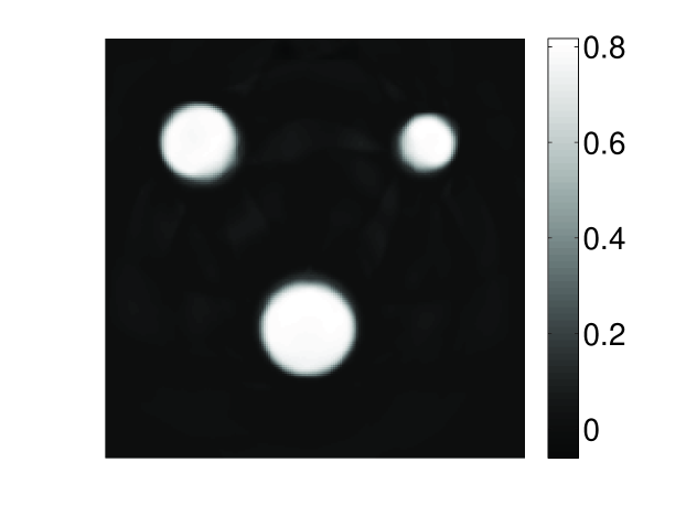
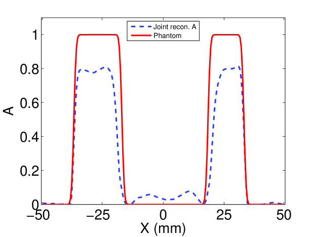
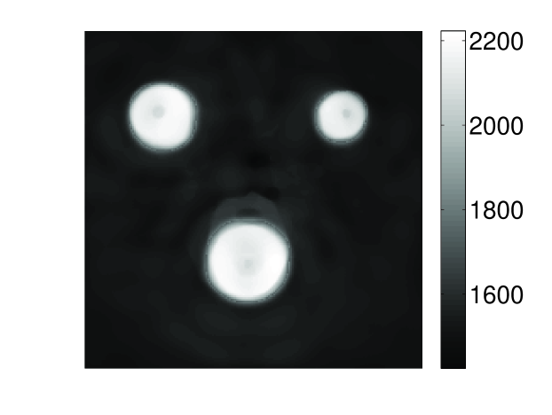
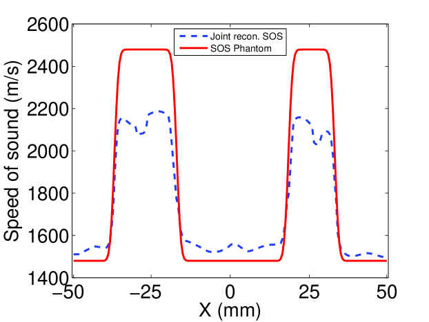
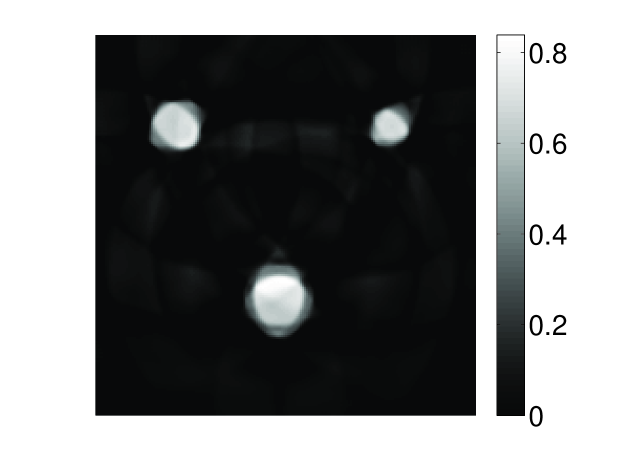
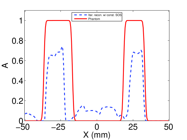
Figure 17: Images obtained via JR from noisy PA measurements in the presence of model error: The top and middle rows display the reconstructed estimates of $\mathbf{A}$ and $\mathbf{c}$, respectively, along with the corresponding image profiles. The bottom row displays an estimate of $\mathbf{A}$ reconstructed by a PACT reconstruction method that employed a constant SOS that was manually tuned to minimize RMSE.

VII Conclusion and discussion

Because variations in the SOS distribution induce aberrations in the measured PA wavefields, certain information regarding an object’s SOS distribution is encoded in the PACT measurement data. As such, several investigators have proposed a JR problem in which the SOS distribution is concurrently estimated along with the sought-after absorbed optical energy density. The purpose of this work was to contribute to a broader understanding of the extent to which this problem can be accurately and reliably solved under realistic conditions. This was accomplished by conducting a series of numerical experiments that elucidated some important numerical properties of the JR problem. These studies demonstrated the numerical instability of the JR problem.

The presented findings are consistent with and corroborate previous theoretical studies of the JR problem. Namely, Stefanov et al proved the instability of the linearized JR problem, which suggested instability of the more general JR problem as well [30]. In [51], a condition for unique reconstruction of $c(\mathbf{r})$ given $A(\mathbf{r})$ was provided, which is consistent with our support condition (see Theorem 3.3 therein). In previous work regarding the development of JR algorithms, Chen et al proposed a similar optimization-based approach to JR [26]. They solved the optimization problem by use of an optimization algorithm called the TR adjoint method. Although their algorithm was different from ours, they obtained similar results; Accurate JR images were not produced when $\mathbf{A}$ is deficient, but the jointly reconstructed $\mathbf{A}$ could be more accurate than the one reconstructed by use of the TR method with a constant SOS.

Similar and results can be found in the works by Jiang et al [24, 25], in which the authors proposed an optimization approach to JR that was based on the Helmholtz equation instead of the wave equation. By use of that method, the authors observed that the accuracy of JR results was affected by the temporal frequency band employed in the reconstruction. Specifically, the frequency ranges covering lower frequencies gave more accurate JR results than higher frequencies. This observation is implicitly contained in our heuristic k-space conjecture. Their observations and our k-space conjecture can be understood by noting that band-pass or high-pass filtered $\mathbf{A}$ are not physical because the non-negativity of $\mathbf{A}$ does not hold in those cases. Both results showed that the accuracy of JR is impacted by the spatial spectrum of $\mathbf{A}$. When $\mathbf{A}$ and $\mathbf{c}$ possess sharp boundaries and the same structures (i.e., are simply scaled versions of each other), the authors also showed that biased estimates of $\mathbf{A}$ and $\mathbf{c}$ could be jointly reconstructed by incorporating Marquardt and Tikhonov regularizations into the reconstruction method. Note that in this case, $\mathbf{A}$ and $\mathbf{c}$ satisfied our support and k-space conjectures. By use of regularization, the authors showed that their algorithm was insensitive to random noise in the measurement, which is congruous with our observations. Although the reconstructed images were biased, the authors showed that the jointly reconstructed $\mathbf{A}$ was more accurate than the image reconstructed with a homogeneous SOS, which is consistent with our results. In addition, they also observed that the jointly reconstructed $\mathbf{A}$ was more accurate than the jointly reconstructed $\mathbf{c}$, which, again, indicated the inverse problem of reconstructing $\mathbf{c}$ is more unstable compared to the reconstruction of $\mathbf{A}$.

However, none of these works reported a systematic investigation of the numerical properties of the JR problem or provided broad insights that allow one to predict when accurate JR may be possible. In particular, the impact of the spatial support and spatial frequency content of $A(\mathbf{r})$ relative to that of $c(\mathbf{r})$ was not explored. In the current study, we have demonstrated that, even if the measurement data are perfect, accurate JR may not be achievable.

The investigation of the JR problem by use of experimental data remains a topic for future investigation. However, based on the presented studies, the task of performing accurate JR under experimental conditions is likely to be highly challenging and will require accurate modeling of the imaging operator. This will generally require the use of the 3D wave equation instead of 2D wave equation. A line search is inevitable in any nonlinear optimization algorithm that is employed to solve Sub-Problem #2, which will create a very large computational burden in the 3D case. Additionally, in this study, a lossless fluid medium was assumed by the reconstruction method. However, in certain applications, density variations and/or acoustic absorption may not be negligible [9, 52]. These assumptions can, in principle, be relaxed when formulating the JR problem.

Finally, due to its instability, it will likely be beneficial to incorporate additional information into the JR problem. One possibility is to augment the PACT measurement data with a small number of ultrasound computed tomography (USCT) measurements. The investigation of the JR problem by combining PACT and USCT measurements is underway [53].

Appendix: calculating the gradient of (15)

The gradient of the first term in Eq. (15) can be calculated by discretizing the the Fréchet derivative (7)

$$\begin{split}\frac{\partial\|\mathbf{H}(\mathbf{c})\mathbf{A}-\hat{\mathbf{p}}\|^{2}}{\partial\mathbf{c}}=-4\mathbf{C}^{-3}\circ\big{\{}\sum_{l=1}^{L-2}\frac{\mathbf{p}_{l+1}-\mathbf{p}_{l-1}}{2}\\ \circ\frac{\mathbf{q}_{l+1}-\mathbf{q}_{l-1}}{2}+(\mathbf{p}_{1}-\mathbf{p}_{0})\circ(\mathbf{q}_{1}-\mathbf{q}_{0})\\ +(\mathbf{p}_{L-1}-\mathbf{p}_{L-2})\circ(\mathbf{q}_{L-1}-\mathbf{q}_{L-2})\big{\}}\end{split}$$ (18)

where $\circ$ denotes Hadamard product, $\mathbf{C}^{-3}$ is defined as

$$\mathbf{C}^{-3}\equiv[c(\mathbf{r}_{1})^{-3},\cdots,c(\mathbf{r}_{N})^{-3}]^{\rm T},$$ (19)

$\mathbf{p}_{l}$ and $\mathbf{q}_{l}$ ($l=0,\cdots,L-1$) are defined as

$$\mathbf{p}_{l}\equiv[p(\mathbf{r}_{1},l\Delta t),\cdots,p(\mathbf{r}_{N},l\Delta t)]^{\rm T},$$ (20)

and

$$\mathbf{q}_{l}\equiv[q(\mathbf{r}_{1},l\Delta t),\cdots,q(\mathbf{r}_{N},l\Delta t)]^{\rm T},$$ (21)

representing the PA wavefield and the adjoint wavefield sampled at the 3D Cartesian grid vertices $\mathbf{r}_{n}$ ($n=1,\cdots,N$) and at time $t=l\Delta t$, respectively.

If TV-penalty is adopted, the gradient of the second term in (15) is given by [54]

$$\frac{\partial\lambda_{c}|\mathbf{c}|_{\text{TV}}}{\partial\mathbf{c}}=\lambda_{c}[\dot{c}_{1},\cdots,\dot{c}_{n},\cdots,\dot{c}_{N}]^{\rm T},$$ (22)

and

$$\begin{split}&\dot{c}_{n}\equiv{(3[\mathbf{c}]_{n}-\sum_{i=1}^{3}[\mathbf{c}]_{n_{i}^{-}})}{\{\epsilon+\sum_{i=1}^{3}([\mathbf{c}]_{n}-[\mathbf{c}]_{n_{i}^{-}})^{2}\}^{-\frac{1}{2}}}\\ &-\sum_{i=1}^{3}{([\mathbf{c}]_{n_{i}^{+}}-[\mathbf{c}]_{n})}{\{\epsilon+\sum_{j=1}^{3}([\mathbf{c}]_{n_{i}^{+}}-[\mathbf{c}]_{{(n_{i}^{+})}_{j}^{-}})^{2}\}^{-\frac{1}{2}}}\\ \end{split}$$ (23)

where $\epsilon$ is a small positive number to prevent the denominators being zeros, and $[\mathbf{c}]_{n}$ denotes the $n$-th grid node of $\mathbf{c}$, and $[\mathbf{c}]_{n_{i}^{-}}$ and $[\mathbf{c}]_{n_{i}^{+}}$ are neighboring nodes before and after the $n$-th node along the $i$-th dimension ($i=1,2,3$), respectively. Likewise, $[\mathbf{c}]_{{(n_{i}^{+})}_{j}^{-}}$ denotes the neighboring node that is after the $n$-th node along the $i$-th dimension and before the $n$-th node along the $j$-th dimension.

The gradient of the objective function in (15) is then given by the sum of Eqs.  (18) and (22).

References

- [1] L. V. Wang, “Photoacoustic imaging and spectroscopy,” in Photoacoustic Imaging and Spectroscopy. CRC, 2009.
- [2] A. A. and A. A. Karabutov, “Optoacoustic tomography,” in Biomedical Photonics Handbook, T. Vo-Dinh, Ed. CRC Press LLC, 2003.
- [3] M. Xu and L. V. Wang, “Photoacoustic imaging in biomedicine,” Review of Scientific Instruments, vol. 77, no. 041101, 2006.
- [4] Y. Xu, D. Feng, and L. V. Wang, “Exact frequency-domain reconstruction for thermoacoustic tomography: I. Planar geometry,” IEEE Transactions on Medical Imaging, vol. 21, pp. 823–828, 2002.
- [5] Y. Xu and L. V. Wang, “Universal back-projection algorithm for photoacoustic computed tomography,” Physical Review E, vol. 71, no. 016706, 2005.
- [6] D. Finch, S. Patch, and Rakesh, “Determining a function from its mean values over a family of spheres,” SIAM Journal of Mathematical Analysis, vol. 35, pp. 1213–1240, 2004.
- [7] L. A. Kunyansky, “Explicit inversion formulae for the spherical mean radon transform,” Inverse Problems, vol. 23, pp. 373–383, 2007.
- [8] K. Wang and M. A. Anastasio, “A simple fourier transform-based reconstruction formula for photoacoustic computed tomography with a circular or spherical measurement geometry,” Physics in Medicine and Biology, vol. 57, no. 23, p. N493, 2012. [Online]. Available: http://stacks.iop.org/0031-9155/57/i=23/a=N493
- [9] C. Huang, L. Nie, R. W. Schoonover, Z. Guo, C. O. Schirra, M. A. Anastasio, and L. V. Wang, “Aberration correction for transcranial photoacoustic tomography of primates employing adjunct image data,” Journal of Biomedical Optics, vol. 17, no. 6, p. 066016, 2012. [Online]. Available: http://link.aip.org/link/?JBO/17/066016/1
- [10] Y. Xu and L. Wang, “Effects of acoustic heterogeneity in breast thermoacoustic tomography,” Ultrasonics, Ferroelectrics and Frequency Control, IEEE Transactions on, vol. 50, no. 9, pp. 1134 –1146, Sept. 2003.
- [11] D. Modgil, M. A. Anastasio, and P. J. La Rivière, “Image reconstruction in photoacoustic tomography with variable speed of sound using a higher-order geometrical acoustics approximation,” Journal of Biomedical Optics, vol. 15, no. 2, pp. 021 308–021 308–9, 2010. [Online]. Available: + http://dx.doi.org/10.1117/1.3333550
- [12] J. Jose, R. G. H. Willemink, S. Resink, D. Piras, J. C. G. van Hespen, C. H. Slump, W. Steenbergen, T. G. van Leeuwen, and S. Manohar, “Passive element enriched photoacoustic computed tomography (per pact) for simultaneous imaging of acoustic propagation properties and light absorption,” Optics Express, vol. 19, no. 3, pp. 2093–2104, Jan 2011. [Online]. Available: http://www.opticsexpress.org/abstract.cfm?URI=oe-19-3-2093
- [13] Z. Yuan and H. Jiang, “Three-dimensional finite-element-based photoacoustic tomography: Reconstruction algorithm and simulations,” Medical Physics, vol. 34, no. 2, pp. 538–546, 2007. [Online]. Available: http://link.aip.org/link/?MPH/34/538/1
- [14] Y. Hristova, P. Kuchment, and L. Nguyen, “Reconstruction and time reversal in thermoacoustic tomography in acoustically homogeneous and inhomogeneous media,” Inverse Problems, vol. 24, no. 5, p. 055006, 2008. [Online]. Available: http://stacks.iop.org/0266-5611/24/i=5/a=055006
- [15] P. Stefanov and G. Uhlmann, “Thermoacoustic tomography with variable sound speed,” Inverse Problems, vol. 25, no. 7, p. 075011, 2009. [Online]. Available: http://stacks.iop.org/0266-5611/25/i=7/a=075011
- [16] C. Huang, K. Wang, L. Nie, L. V. Wang, and M. A. Anastasio, “Full-wave iterative image reconstruction in photoacoustic tomography with acoustically inhomogeneous media,” Medical Imaging, IEEE Transactions on, vol. 32, no. 6, pp. 1097–1110, 2013.
- [17] X. L. Deán-Ben, V. Ntziachristos, and D. Razansky, “Statistical optoacoustic image reconstruction using a-priori knowledge on the location of acoustic distortions,” Applied Physics Letters, vol. 98, no. 17, p. 171110, 2011. [Online]. Available: http://link.aip.org/link/?APL/98/171110/1
- [18] Z. Zhang, L. Huang, and Y. Lin, “Efficient implementation of ultrasound waveform tomography using source encoding,” Proceedings of the SPIE, vol. 8320, pp. 832 003–832 003–10, 2012.
- [19] C. Li, N. Duric, P. Littrup, and L. Huang, “In vivo breast sound-speed imaging with ultrasound tomography,” Ultrasound in Medicine & Biology, vol. 35, no. 10, pp. 1615 – 1628, 2009. [Online]. Available: http://www.sciencedirect.com/science/article/pii/S0301562909002373
- [20] G. Glover, “Characterization of in vivo breast tissue by ultrasonic time-of-flight computed tomography,” in Natl Bur Stand Int Symp Ultrason Tissue Characterization, National Science Foundation, Ultrasonic Tissue Characterization II, 1979, pp. 221–225.
- [21] J. S. Schreiman, J. J. Gisvold, J. F. Greenleaf, and R. C. Bahn, “Ultrasound transmission computed tomography of the breast.” Radiology, vol. 150, no. 2, pp. 523–530, 1984, pMID: 6691113. [Online]. Available: http://pubs.rsna.org/doi/abs/10.1148/radiology.150.2.6691113
- [22] K. Wang, T. Matthews, F. Anis, C. Li, N. Duric, and M. A. Anastasio, “Waveform inversion with source encoding for breast sound speed reconstruction in ultrasound computed tomography,” Ultrasonics, Ferroelectrics, and Frequency Control, IEEE Transactions on, vol. 62, no. 3, pp. 475–493, 2015.
- [23] J. Zhang, K. Wang, Y. Yang, and M. A. Anastasio, “Simultaneous reconstruction of speed-of-sound and optical absorption properties in photoacoustic tomography via a time-domain iterative algorithm,” Proceedings of the SPIE, vol. 6856, 2008.
- [24] H. Jiang, Z. Yuan, and X. Gu, “Spatially varying optical and acoustic property reconstruction using finite-element-based photoacoustic tomography,” Journal of the Optical Society of America A, vol. 23, no. 4, pp. 878–888, Apr 2006. [Online]. Available: http://josaa.osa.org/abstract.cfm?URI=josaa-23-4-878
- [25] Z. Yuan, Q. Zhang, and H. Jiang, “Simultaneous reconstruction of acoustic and optical properties of heterogeneous media by quantitative photoacoustic tomography,” Optics Express, vol. 14, no. 15, pp. 6749–6754, Jul 2006.
- [26] G. Chen, X. Wang, J. Wang, Z. Zhao, Z. Nie, and Q. Liu, “Tr adjoint imaging method for mitat,” Progress In Electromagnetics Research B, vol. 46, pp. 41–57, 2013.
- [27] A. Kirsch and O. Scherzer, “Simultaneous reconstructions of absorption density and wave speed with photoacoustic measurements,” SIAM Journal on Applied Mathematics, vol. 72, no. 5, pp. 1508–1523, 2012.
- [28] K. S. Hickmann, “Unique determination of acoustic properties from thermoacoustic data,” Ph.D. dissertation, Oregon State University, 2010.
- [29] A. Kirsch and O. Scherzer, “Simultaneous reconstructions of absorption density and wave speed with photoacoustic measurements,” SIAM Journal on Applied Mathematics, vol. 72, no. 5, pp. 1508–1523, 2012.
- [30] P. Stefanov and G. Uhlmann, “Instability of the linearized problem in multiwave tomography of recovery both the source and the speed.” Inverse Problems & Imaging, vol. 7, no. 4, 2013.
- [31] C. Bunks, F. Saleck, S. Zaleski, and G. Chavent, “Multiscale seismic waveform inversion,” Geophysics, vol. 60, no. 5, pp. 1457–1473, 1995. [Online]. Available: http://library.seg.org/doi/abs/10.1190/1.1443880
- [32] S. J. Norton, “Iterative inverse scattering algorithms: Methods of computing fréchet derivatives,” The Journal of the Acoustical Society of America, vol. 106, no. 5, pp. 2653–2660, 1999. [Online]. Available: http://link.aip.org/link/?JAS/106/2653/1
- [33] B. E. Treeby, E. Z. Zhang, and B. T. Cox, “Photoacoustic tomography in absorbing acoustic media using time reversal,” Inverse Problems, vol. 26, no. 11, p. 115003, 2010. [Online]. Available: http://stacks.iop.org/0266-5611/26/i=11/a=115003
- [34] F. Natterer, “The mathematics of computerized tomography,” in The Mathematics of Computerized Tomography. Society for Industrial and Applied Mathematics, 2001.
- [35] B. Treeby and B. Cox, “k-wave: MATLAB toolbox for the simulation and reconstruction of photoacoustic wave fields,” Journal of Biomedical Optics, vol. 15, p. 021314, 2010.
- [36] D. M. Dunlavy, T. G. Kolda, and E. Acar, “Poblano v1.0: A matlab toolbox for gradient-based optimization,” Sandia National Laboratories, Albuquerque, NM and Livermore, CA, Tech. Rep. SAND2010-1422, Mar. 2010.
- [37] J. E. Dennis, Jr. and R. B. Schnabel, “Numerical methods for unconstrained optimization and nonlinear equations,” in Numerical Methods for Unconstrained Optimization and Nonlinear Equations. Society for Industrial and Applied Mathematics, 1996.
- [38] J. Nocedal and S. J. Wright, “Numerical optimization,” in Numerical Optimization. Springer, 1999.
- [39] B. Zhang, S. Xu, F. Zhang, Y. Bi, and L. Huang, “Accelerating matlab code using gpu: A review of tools and strategies,” in Artificial Intelligence, Management Science and Electronic Commerce (AIMSEC), 2011 2nd International Conference on, aug. 2011, pp. 1875 –1878.
- [40] K. Wang, S. A. Ermilov, R. Su, H.-P. Brecht, A. A. Oraevsky, and M. A. Anastasio, “An imaging model incorporating ultrasonic transducer properties for three-dimensional optoacoustic tomography,” Medical Imaging, IEEE Transactions on, vol. 30, no. 2, pp. 203 –214, feb. 2011.
- [41] A. Rosenthal, V. Ntziachristos, and D. Razansky, “Model-based optoacoustic inversion with arbitrary-shape detectors,” Medical physics, vol. 38, no. 7, pp. 4285–4295, 2011.
- [42] Q. Sheng, K. Wang, J. Xia, L. Zhu, L. V. Wang, and M. A. Anastasio, “Photoacoustic computed tomography without accurate ultrasonic transducer responses,” in SPIE BiOS. International Society for Optics and Photonics, 2015, pp. 932 313–932 313.
- [43] P. J. L. Rivière, J. Zhang, and M. A. Anastasio, “Image reconstruction in optoacoustic tomography for dispersive acoustic media,” Optics Letters, vol. 31, no. 6, pp. 781–783, Mar 2006. [Online]. Available: http://ol.osa.org/abstract.cfm?URI=ol-31-6-781
- [44] X. L. Deán-Ben, D. Razansky, and V. Ntziachristos, “The effects of acoustic attenuation in optoacoustic signals,” Physics in Medicine and Biology, vol. 56, no. 18, p. 6129, 2011. [Online]. Available: http://stacks.iop.org/0031-9155/56/i=18/a=021
- [45] T. L. Szabo, “Time domain wave equations for lossy media obeying a frequency power law,” The Journal of the Acoustical Society of America, vol. 96, no. 1, pp. 491–500, 1994. [Online]. Available: http://dx.doi.org/doi/10.1121/1.410434
- [46] ——, “Diagnostic ultrasound imaging,” in Diagnostic Ultrasound Imaging: Inside Out. Elsevier, 2004.
- [47] G. R. Harris, “Review of transient field theory for a baffled planar piston,” The Journal of the Acoustical Society of America, vol. 70, no. 1, pp. 10–20, 1981. [Online]. Available: http://link.aip.org/link/?JAS/70/10/1
- [48] A. Conjusteau, S. A. Ermilov, R. Su, H.-P. Brecht, M. P. Fronheiser, and A. A. Oraevsky, “Measurement of the spectral directivity of optoacoustic and ultrasonic transducers with a laser ultrasonic source,” Review of Scientific Instruments, vol. 80, no. 9, pp. –, 2009. [Online]. Available: http://scitation.aip.org/content/aip/journal/rsi/80/9/10.1063/1.3227836
- [49] K. Wang, R. Su, A. A. Oraevsky, and M. A. Anastasio, “Sparsity regularized data-space restoration in optoacoustic tomography,” Proceedings of the SPIE, vol. 8223, pp. 822 322–822 322–7, 2012.
- [50] X. Zhu, Z. Zhao, J. Wang, G. Chen, and Q. H. Liu, “Active adjoint modeling method in microwave induced thermoacoustic tomography for breast tumor,” Biomedical Engineering, IEEE Transactions on, vol. 61, no. 7, pp. 1957–1966, 2014.
- [51] P. Stefanov and G. Uhlmann, “Recovery of a source term or a speed with one measurement and applications,” Transactions of the American Mathematical Society, vol. 365, no. 11, pp. 5737–5758, 2013.
- [52] C. Huang, L. Nie, R. W. Schoonover, L. V. Wang, and M. A. Anastasio, “Photoacoustic computed tomography correcting for heterogeneity and attenuation,” Journal of Biomedical Optics, vol. 17, no. 6, p. 061211, 2012. [Online]. Available: http://link.aip.org/link/?JBO/17/061211/1
- [53] T. P. Matthews, K. Wang, L. V. Wang, and M. A. Anastasio, “Synergistic image reconstruction for hybrid ultrasound and photoacoustic computed tomography,” in SPIE BiOS. International Society for Optics and Photonics, 2015, pp. 93 233A–93 233A.
- [54] E. Y. Sidky, C.-M. Kao, and X. Pan, “Accurate image reconstruction from few-views and limited-angle data in divergent-beam ct,” Journal of X-Ray Science and Technology, vol. 14, no. 2, p. 119, 2006.