Dynamics of fully coupled rotators with unimodal and bimodal frequency distribution

Abstract

We analyze the synchronization transition of a globally coupled network of $N$ phase oscillators with inertia (rotators) whose natural frequencies are unimodally or bimodally distributed. In the unimodal case, the system exhibits a discontinuous hysteretic transition from an incoherent to a partially synchronized (PS) state. For sufficiently large inertia, the system reveals the coexistence of a PS state and of a standing wave (SW) solution. In the bimodal case, the hysteretic synchronization transition involves several states. Namely, the system becomes coherent passing through traveling waves (TWs), SWs and finally arriving to a PS regime. The transition to the PS state from the SW occurs always at the same coupling, independently of the system size, while its value increases linearly with the inertia. On the other hand the critical coupling required to observe TWs and SWs increases with $N$ suggesting that in the thermodynamic limit the transition from incoherence to PS will occur without any intermediate states. Finally a linear stability analysis reveals that the system is hysteretic not only at the level of macroscopic indicators, but also microscopically as verified by measuring the maximal Lyapunov exponent.

0.1 Introduction

The renowned Kuramoto model [14] for phase oscillators was generalized in 1997 by Tanaka, Lichtenberg and Oishi (TLO)[24, 25] by including an additional inertial term. The TLO model revealed, at variance with the usual Kuramoto model, first order synchronization transitions even for unimodal distributions of the natural frequencies. TLO have been inspired in their extension by a work of Ermentrout published in 1991 [7]; in this paper Ermentrout has introduced a pulse coupled phase oscillator model with inertia to mimic the perfect synchrony achieved by a specific type of fireflies, the Pteroptix Malaccae (but also by certain species of crickets and humans). The peculiarity of these fireflies is that they are able to synchronize their flashing activity to some forcing frequency (even quite distinct from their own intrinsic flashing frequency) with an almost zero phase lag. This happens because they adapt their period of oscillation to that of the driving oscillator. After his introduction, the Kuramoto model with inertia has been employed to describe synchronization phenomena in crowd synchrony on London’s Millennium bridge [23], as well as in Huygen’s pendulum clocks [4]. Furthermore, phase oscillators with inertia (rotators) have recently found application in the study the self-synchronization in power and smart grids  [21, 8, 20, 6, 16], as well as in the analysis of disordered arrays of underdamped Josephson junctions [26]. Cluster explosive synchronization has been reported for an adaptive network of Kuramoto oscillators with inertia, where the natural frequency of each oscillator is assumed to be proportional to the degree of the corresponding node [12]. Rotators arranged in two symmetrically coupled populations have recently revealed the emergence of intermittent chaotic chimeras [17], imperfect chimera states have been found in a ring with nonlocal coupling [11], and transient waves have been observed in regular lattices [13].

There is a wide literature devoted to coupled rotators  with an unimodal frequency distribution, however only a really limited number of studies have been devoted to this model with a bimodal distribution, despite the subject being extremely relevant for the modelization of the power grids  [8, 20, 18]. To our knowledge the synchronization transition in populations of globally coupled rotators with bimodal distribution has been previously analyzed only by Acebrón et al. in [1]. More specifically, the authors considered a model with white noise and a distribution composed by two $\delta$-functions localized at $\pm\Omega_{0}$. As suggested in [15], the presence of noise blurs the $\delta$-functions in bell-shaped functions analogous to Gaussian distributions. Therefore one expects a similar phenomenology to the one observable for deterministic systems with bimodal Gaussian distributions of the frequencies. A multiscale analysis of the model, in the limit of sufficiently large $\Omega_{0}$, reveals the emergence from the incoherent state of stable standing wave solutions (SWs)  and of unstable traveling wave solutions (TWs)  via supercritical bifurcations, while partially synchronized stationary states (PSs)  bifurcates subcritically from incoherence. However, the authors affirm that in the considered limit the bifurcation diagram coincides with that of the usual Kuramoto model without inertia  [2].

In this article we analyze the synchronization transitions observable for unimodal and bimodal frequency distributions for a population of globally coupled rotators in a fully deterministic system. In particular, we will analyze the influence of inertia and of finite size effects on the synchronization transitions. Moreover, we will study the macroscopic and microscopic characteristics of the different regimes emerging during adiabatic increase and decrease of the coupling among the rotators. In particular, Section 1.2 will be devoted to the introduction of the model, of the indicators used to characterize the synchronization transition, and of the different protocols employed to perform adiabatic simulations. The Lyapunov linear stability analysis is introduced in SubSection 1.2.1. The results for unimodal distributions are reported in Sect. 1.3, with a particular emphasis to the TLO mean field theory and its extension to any generic state observable within the hysteretic region (SubSect. 1.3.2). The emergence of clusters of locked and whirling oscillators is described in details in SubSect. 1.3.3. The dynamics of the network for bimodal distributions is analyzed in Section 1.4. In particular, SubSect. 1.4.1 is devoted to two non overlapping distributions and SubSect. 1.4.2 to largely overlapping Gaussian distributions. Sect. 1.5 report the result of linear stability analysis for the considered distributions. Finally, in Sect. 1.6 the reported results are briefly summarized and discussed.

0.2 Model and Indicators

By following Refs. [25, 24], we study the following version of the Kuramoto model with inertia for $N$ fully coupled rotators :

$$m\ddot{\theta}_{i}+\dot{\theta}_{i}=\Omega_{i}+\frac{K}{N}\sum_{j}\sin(\theta_{j}-\theta_{i})$$ (1)

where $\theta_{i}$ and $\Omega_{i}$ are, respectively, the instantaneous phase and the natural frequency of the $i$-th oscillator, $K$ is the coupling. In the following we will consider random natural frequencies $\Omega_{i}$ Gaussian distributed according to: an unimodal distribution $g(\Omega)=\frac{1}{\sqrt{2\pi}}{\rm e}^{-\frac{\Omega^{2}}{2}}$ with zero average and an unitary standard deviation or a bimodal symmetric distribution $g(\Omega)=\frac{1}{2\sqrt{2\pi}}\left[{\rm e}^{-\frac{(\Omega-\Omega_{0})^{2}}{2}}+{\rm e}^{-\frac{(\Omega+\Omega_{0})^{2}}{2}}\right]$, which is the overlap of two Gaussians with unitary standard deviation and with the peaks located at a distance $2\Omega_{0}$.

To measure the level of coherence between the oscillators, we employ the complex order parameter  [27]

$$r(t)e^{i\phi(t)}=\frac{1}{N}\sum_{j}e^{i\theta_{j}}\enskip;$$ (2)

where $r(t)\in[0:1]$ is the modulus and $\phi(t)$ the phase of the macroscopic indicator. An asynchronous state, in a finite network, is characterized by $r\simeq\frac{1}{\sqrt{N}}$, while for $r\equiv 1$ the oscillators are fully synchronized and intermediate $r$-values correspond to partial synchronization.

Another relevant indicator for the state of the rotator population is the number of locked oscillators $N_{L}$, characterized by a vanishingly small average phase velocity $\bar{\omega_{i}}\equiv\bar{\frac{d{\theta_{i}}}{dt}}$, and the maximal locking frequency $\Omega_{M}$, which corresponds to the maximal natural frequency $|\Omega_{i}|$ of the locked oscillators.

In general we will perform sequences of simulations by varying adiabatically the coupling parameter $K$ with two different protocols. Namely, for the first protocol (I) the series of simulations is initialized for the decoupled system by considering random initial conditions for $\{\theta_{i}\}$ and $\{\omega_{i}\}$. Afterwards the coupling is increased in steps $\Delta K$ until a maximal coupling $K_{M}$ is reached. For each value of $K$, apart the very first one, the simulations is initialized by employing the last configuration of the previous simulation in the sequence. For the second protocol (II), starting from the final coupling $K_{M}$ achieved by employing the protocol (I), the coupling is reduced in steps $\Delta K$ until $K=0$ is recovered. At each step the system is simulated for a transient time $T_{R}$ followed by a period $T_{W}$ during which the average value of the order parameter ${\bar{r}}$ and of the velocities $\{\bar{\omega_{i}}\}$, as well as $\Omega_{M}$, are estimated.

0.2.1 Lyapunov Analysis

The stability of Eq. (1) can be analyzed by following the evolution of infinitesimal perturbations $\mathcal{T}=(\delta\dot{\theta}_{1},\dots,\delta\dot{\theta}_{N},\delta{\theta}_{1},\dots,\delta{\theta}_{N})$ in the tangent space, whose dynamics is ruled by the linearization of Eq. (1) as follows:

$$m\enskip\delta\ddot{\theta}_{i}+\delta\dot{\theta}_{i}=\frac{K}{N}\sum_{j=1}^{N}\cos{\left(\theta_{j}-\theta_{i}\right)(\delta\theta_{j}-\delta\theta_{i})}\enskip.$$ (3)

We will limit to estimate the maximal Lyapunov exponent $\lambda_{M}$, by employing the method developed by Benettin et al. [3]. This amounts to follow the dynamical evolution of the orbit and of the tangent vector $\mathcal{T}$ for a time lapse $T_{W}$ by performing Gram-Schmidt ortho-normalization at fixed time intervals $\Delta t$, after discarding an initial transient evolution $T_{R}$.

Furthermore, the values of the components of the maximal Lyapunov vector ${\cal T}$ can give important information about the oscillators that are more actively contributing to the chaotic dynamics. It is useful to introduce the following squared amplitude component of the normalized vector for each rotator [9, 17]

$$\xi_{i}(t)=[\delta\dot{\theta}_{i}(t)]^{2}+[\delta{\theta}_{i}(t)]^{2}\enskip,\qquad i=1,\dots,N\enskip.$$ (4)

The time average ${\bar{\xi}_{i}}$ of this quantity gives a measure of the contribution of each oscillator to the chaotic dynamics.

0.3 Unimodal Frequency Distribution

0.3.1 Hysteretic Synchronization Transitions

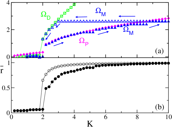
Figure 1: Unimodal frequency distribution. (a) Maximal locking frequency $\Omega_{M}$ (blue triangles) and (b) time averaged order parameter ${\bar{r}}$ (black circles) as a function of the coupling $K$ for two series of simulations performed following the protocol (I) (filled symbols) and the protocol (II) (empty symbols). The data refer to inertia: $m=2$, for which we set $\Delta K=0.2$ and $K_{M}=10$; moreover $N=500$, $T_{R}=5,000$ and $T_{W}=200$. The (magenta) diamonds indicate $\Omega_{P}=\frac{4}{\pi}\sqrt{\frac{K\bar{r}}{m}}$ for protocol (I) and the (green) squares $\Omega_{D}=K\bar{r}$ for protocol (II).

In Fig. 1 the results for a sequence of simulations obtained by following protocol (I) and (II) are reported for a not too small inertia (namely, $m=2$) and unimodal frequency distribution. For the first protocol the system remains incoherent up to a critical value $K=K_{1}^{c}\simeq 2$, where $\bar{r}$ jumps to a finite value and then increases with $K$ reaching $\bar{r}\simeq 1$ for sufficiently large coupling. Starting from the last state and by reducing $K$ one notices that $\bar{r}$ assumes larger values than during protocol (I) and the system becomes incoherent at a smaller coupling, namely $K_{2}^{c}<K_{1}^{c}$. This is a clear indication of the hysteretic nature of the synchronization transition in this case.

For the chosen values of the inertia, we observe the creation of an unique cluster of $N_{L}$ locked oscillators with $\bar{\omega_{i}}\simeq 0$, for larger $m$ the things will be more complex, as we will discuss in the following. The maximal locking frequency $\Omega_{M}$ becomes finite for $K>K_{1}^{c}$ and increases with $K$. The frequency $\Omega_{M}$ attains a maximal value when $\bar{r}\simeq 1$, no more oscillators can be recruited in the large locked cluster. Once reached this value, even if $K$ is reduced following the protocol (II), $\Omega_{M}$ remains constant for a wide $K$ interval. Then $\Omega_{M}$ shows a rapid decrease towards zero by approaching $K_{2}^{c}$. This behavior will be explained in the following two sub-sections.

0.3.2 Mean field theory

In order to derive a mean field description of the dynamics of each single rotator, we can rewrite Eq. (1) by employing the order parameter definition (2) as follows

$$m\ddot{\theta}_{i}+\dot{\theta}_{i}=\Omega_{i}-Kr\sin(\theta_{i}-\phi)\qquad;$$ (5)

this corresponds to the evolution equation for a damped driven pendulum. Eq. (5) admits, for sufficiently small forcing frequency $\Omega_{i}$, two fixed points: a stable node and a saddle. At larger frequencies $\Omega_{i}>\Omega_{P}\simeq\frac{4}{\pi}\sqrt{\frac{Kr}{m}}$ the saddle, via a homoclinic bifurcation, gives rise to a limit cycle. The stable limit cycle and a stable fixed point coexist until a saddle node bifurcation, taking place at $\Omega_{i}=\Omega_{D}=Kr$, leads to the disappearance of the fixed points and for $\Omega_{i}>\Omega_{D}$ only the limit cycle persists. This scenario is correct for sufficiently large inertia; at small $m$ one has a direct transition from a stable node to a periodic oscillating orbit at $\Omega_{i}=\Omega_{D}=Kr$ [22]. Therefore for sufficiently large $m$ there is a coexistence regime where, depending on the initial conditions, the single oscillator can rotate or stay quiet. The fixed point (limit cycle) solution corresponds to locked (drifting) rotators.

The TLO theory [25, 24] has explained the origin of the first order hysteretic transitions by considering two opposite initial states for the network: (I) the completely incoherent phase ($r=0$) and (II) the completely synchronized one ($r\equiv 1$). In case (I) the oscillators are all initially drifting with finite velocities ${\omega_{i}}$; by increasing $K$ the oscillators with smaller natural frequencies $|\Omega_{i}|<\Omega_{P}$ begin to lock ($\bar{\omega_{i}}=0$), while the other continue to drift. This is confirmed by the data reported in Fig. 1, where it is clear that the locking frequency $\Omega_{M}$ is well approximated by $\Omega_{P}$. The process continues until all the oscillators are finally locked, leading to $r=1$ and to a plateau in $\Omega_{M}$.

In the second case, initially all the oscillators are already locked, with an associated order parameter $r\equiv 1$. Therefore, the oscillators can start to drift only when the stable fixed point solution will disappear, leaving the system only with the limit cycle solution. This happens, by decreasing $K$, whenever $|\Omega_{i}|\geq\Omega_{D}=Kr$. This is numerically verified, indeed, as shown in Fig. 1, where it is clear that the maximal locked frequency $\Omega_{M}$ remains constant until, by decreasing $K$, it encounters the curve $\Omega_{D}$ and then $\Omega_{M}$ follows this latter curve down towards the asynchronous state. The case (II) corresponds to the situation observable for the usual Kuramoto model, where there is no bistability [14].

In both the considered cases there is a group of desynchronized oscillators and one of locked oscillators separated by a frequency, $\Omega_{P}$ ($\Omega_{D}$ ) in case (I) (case (II)). At variance with the usual Kuramoto model, both these groups contribute to the total level of synchronization, namely

$$r=r_{L}+r_{D}$$ (6)

where $r_{L}$ ($r_{D}$) is the contribution of the locked (drifting) population.

The contribution of the locked population is simply given by

$$r_{L}^{I,II}=Kr\int_{-\theta_{P,D}}^{\theta_{P,D}}\cos^{2}\theta g(Kr\sin\theta)d\theta\qquad;$$ (7)

where $\theta_{P}=\sin^{-1}(\Omega_{P}/Kr)$ and $\theta_{D}=\sin^{-1}(\Omega_{D}/Kr)\equiv\pi/2$.

The contribution $r_{D}$ of the drifting rotators is negative and it has been estimated analytically by TLO by performing a perturbative expansion to the fourth order in $1/(mK)$ and $1/(m\Omega)$. The obtained expression, valid for sufficiently large inertia, reads as

$$r_{D}^{I,II}\simeq-mKr\int_{\Omega_{P,D}}^{\infty}\frac{1}{(m\Omega)^{3}}g(\Omega)d\Omega\qquad;$$ (8)

with $g(\Omega)=g(-\Omega)$.

By considering an initially desynchronized (fully synchronized) system and by increasing (decreasing) $K$ one can get a theoretical approximation for the level of synchronization in the system by employing the mean-field expression (7), (8) and (6) for case I (II). In this way, two curves are obtained in the phase plane $(K,r)$, namely $r^{I}(K)$ and $r^{II}(K)$. For a certain coupling $K$ the system can attain all the possible levels of synchronization between $r^{I}(K)$ and $r^{II}(K)$.

Let us notice that the expression for $r_{L}$ and $r_{D}$ reported in Eqs. (7) and (8) are the same for case (I) and (II), only the integration extrema change in the two cases. These are defined by the frequency which discriminates locked from drifting neuron, that in case (I) is $\Omega_{P}$ and in case (II) $\Omega_{D}$. It should be noticed that the value of these frequencies is a function of the order parameter $r$ and of the coupling constant $K$, therefore one should solve implicit integrals to obtain $r$.

However, one could also fix the discriminating frequency to some arbitrary value $\Omega_{0}$ and solve self-consistently the equations Eqs. (6), (7), and (8) for different values of the coupling $K$. This corresponds to solve the equation 

$$\int_{-\theta_{0}}^{\theta_{0}}\cos^{2}\theta g(Kr^{0}\sin\theta)d\theta-m\int_{\Omega_{0}}^{\infty}\frac{1}{(m\Omega)^{3}}g(\Omega)d\Omega=\frac{1}{K}\qquad;$$ (9)

with $\theta_{0}=\sin^{-1}(\Omega_{0}/Kr^{0})$. A solution $r^{0}=r^{0}(K,\Omega_{0})$ exists provided that $\Omega_{0}\leq\Omega_{D}(K)=r^{0}K$. Therefore the part of the plane delimited by the curve $r^{II}(K)$, will be filled with the curves $r_{0}(K)$ obtained for different $\Omega_{0}$ values (as shown in Fig. 2(a)). These solutions represent clusters of $N_{L}$ oscillators for which the maximal locking frequency and $N_{L}$ do not vary upon changing the coupling strength. In particular, for $K>K_{2}^{c}$ these states can be observed in numerical simulations in the portion of the phase space delimited by the two curves $r^{I}(K)$ and $r^{II}(K)$ (see Fig. 2(b)).

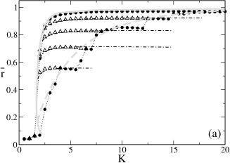
Figure 2: Unimodal Distribution. Panel (a): Average order parameter ${\bar{r}}$ versus the coupling constant $K$. Theoretical mean field estimates: the dashed (solid) grey curves refer to $r^{I}=r^{I}_{L}+r^{I}_{D}$ ($r^{II}=r^{II}_{L}+r^{II}_{D}$) as obtained by employing Eqs. (7) and (8) following protocol (I) (protocol (II)); the (black) dot-dashed curves are the solutions $r^{0}(K,\Omega_{0})$ of Eq. (9) for different $\Omega_{0}$ values. The employed values from bottom to top are: $\Omega_{0}=0.79$, 1.09, 1.31 and 1.79. Numerical simulations: (black) filled circles have been obtained by following protocol (I) and then (II) starting from $K=0$ until $K_{M}=20$ with steps $\Delta K=0.5$; (black) empty triangles refer to simulations performed by starting from a final configuration obtained during protocol (I) and by decreasing the coupling from such initial configurations. The Panel (b) displays $N_{L}$ vs $K$ for the numerical simulations reported in (a). The numerical data refer to $m=6$, $N=500$, $T_{R}=5000$, and $T_{W}=200$.

0.3.3 Clusters of Locked and Whirling Oscillators

By observing the results reported in Fig. 2(a) for $m=6$, it is evident that the numerical data obtained by following the procedure (II) are quite well reproduced from the mean field approximation $r^{II}$ (solid grey curve). This is not the case for the theoretical estimation $r^{I}$ (dashed grey curve), which does not reproduce the step-wise structure revealed for the data corresponding to protocol (I). This step-wise structure emerges only for sufficiently large inertia (as it is clear from Fig. 1 (b), where it is absent for $m=2$); this is due to the break down of the independence of the whirling oscillators: namely, to the formation of clusters of drifting oscillators moving coherently at the same non zero velocity [24]. Oscillators join in small groups to the locked stationary cluster and not individually as it happens for smaller inertia; this is clearly revealed by the behavior of $N_{L}$ versus the coupling $K$ as reported in Fig. 2(b).

Furthermore, once formed, these stationary locked clusters are particularly robust, as it can be appreciated by considering as initial condition a partially synchronized state obtained following protocol (I) for a certain coupling $K_{S}>K_{1}$. This state is characterized by a cluster of $N_{L}$ locked; if now we reduce the coupling $K$, the number of locked oscillators remain constant until we do not reach the descending curve obtained with protocol (II), see the black empty triangles in Fig. 2. On the other hand $\bar{r}$ decreases slightly with $K$, this behavior is well reproduced by the mean field solutions of Eq. (9), namely $r^{0}(K,\Omega_{0})$ with $\Omega_{0}=\Omega_{P}(K_{s},r^{I}(K_{S}))=\frac{4}{\pi}\sqrt{\frac{K_{s}r^{I}}{m}}$, these are shown in Fig. 2 (a) as black dot-dashed lines. As soon as, by decreasing $K$, the frequency $\Omega_{0}$ becomes equal or smaller than $\Omega_{D}$, the order parameter has a rapid drop towards zero following the upper limit curve $r^{II}$. These results indicate that hysteretic loops of any size are possible within the region delimited by the two curves $\bar{r}$ obtained by following protocol I and II respectively, as shown in [18].

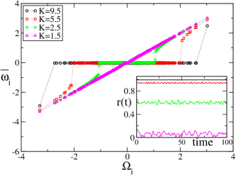
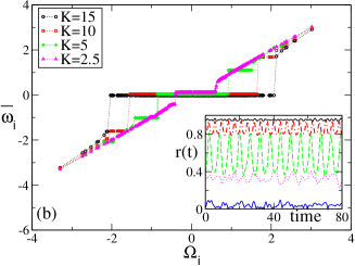
Figure 3: Unimodal Distribution. Average phase velocity $\bar{\omega_{i}}$ of the rotators versus their natural frequencies $\Omega_{i}$ for $N=500$ and inertia $m=2$ (a) and $m=6$ (b). In panel (a) (panel (b)) magenta triangles refer to $K=1.5$ ($K=2.5$), green diamonds to $K=2.5$ ($K=5$), red squares to $K=5.5$ ($K=10$) and black circles to $K=9.5$ ($K=15$). The insets report the time evolution of the order parameters $r(t)$ for the corresponding coupling constants, apart for the extra blue line shown in the inset in (b) which refers to $K=1$. For each simulation an initial transient $T_{R}\simeq 5,500$ has been discarded and the time averages have been estimated over a window $T_{W}=5,000$.

For sufficiently small $m$, the synchronization occurs starting from the incoherent state via the formation of an unique cluster of locked oscillators, and the size of this cluster increases with $K$, as evident from Fig. 3 (a) for $m=2$. At the same time the value of $r$ also increases with $K$ and its evolution is characterized only by finite size fluctuations vanishing in the thermodynamic limit (see the inset of Fig. 3 (a)). As already mentioned, the situation is different for sufficiently large inertia, now the partially synchronized phase is characterized by the coexistence of the main cluster of locked oscillators with $\bar{\omega_{i}}\simeq 0$, but also by the emergence of clusters composed by drifting oscillators with common finite velocities, see the data for $\bar{\omega_{i}}$ reported in Fig. 3 (b) for $m=6$. In particular, the clusters of whirling oscillators emerge always in couple and they are characterized by the same average velocity but opposite sign. These states are indicated as standing waves (SWs), therefore we have a SW coexisting with a partially synchronized stationary state (PS) (as shown in Fig. 3 (b).

The effect of these extra clusters on the collective dynamics is to induce oscillations in the temporal evolution of the order parameter, as one can see from the inset of Fig.  3 (b). In presence of drifting clusters characterized by the same average velocity (in absolute value), as for $m=6$ and $K=5$ in Fig.  3 (b), $r$ exhibits almost regular oscillations and the period of these oscillations corresponds to the one associated to the oscillators in the drifting cluster.

0.4 Bimodal Distribution

In this Section we consider a bimodal distribution, we will initially focus on two almost non overlapping Gaussians, namely we consider $\Omega_{0}=2$, while Sub-Section 1.4.2 is devoted to overlapping Gaussians, examined for $\Omega_{0}=0.2$.

0.4.1 Non Overlapping Gaussians

For $\Omega_{0}=2$ and sufficiently small inertia ($m=1$ and 2), we observe a very rich synchronization transition, as shown in Fig. 4 (a). In particular, by following protocol (I) we observe that the system leaves the incoherent state abruptly by exhibiting a jump to a finite $\bar{r}$ value at $K^{TW}$; above such value in the network emerges a single cluster of oscillators, drifting together with a finite velocity $\simeq\Omega_{0}$, this corresponds to Traveling Wave (TW) solution . By further increasing $K$ a second finite jump of the order parameter at $K^{SW}$ denotes the passage to a Standing Wave (SW)  solution, corresponding to two clusters of drifting oscillators with symmetric opposite velocities $\simeq\pm\Omega_{0}$. A final jump at $K^{PS}$ leads the system to a Partially Synchronized (PS)  phase, characterized by an unique cluster of locked rotators  with zero average velocity. By increasing the coupling the PS state smoothly approaches the fully synchronized regime . Starting from this final state the return sequence of simulations, following protocol (II), displays a simpler phenomenology. The network stays in the PS regime, characterized by an order parameter larger than that measured during protocol (I) simulations, until $K^{DS}<K^{TW}$. For smaller coupling, the system leaves the PS state; however, depending on the realization of the natural frequencies and on the initial conditions, it can ends up or in a TW (most of the cases) or in a SW, or it can even reach directly the incoherent state (as shown in Fig. 4 (a) and Fig. 6 (a)). This first analysis clearly shows hysteretic effects and coexistence of macroscopic states with different level of synchronization for a wide range of couplings.

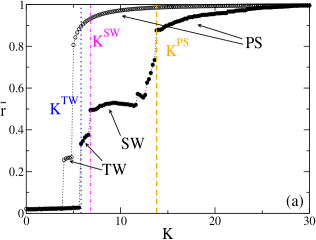
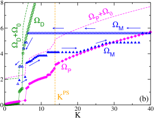
Figure 4: Bimodal frequency distribution. Panel (a): Average order parameter ${\bar{r}}$ versus $K$ for two series of simulations performed following the protocol (I) (filled symbols) and (II) (empty symbols). The dotted vertical blue line refers to $K^{TW}$; the dashed-dotted magenta line to $K^{SW}$. Panel (b): Maximal locking frequency $\Omega_{M}$ (blue triangles) versus $K$ for simulations reported in (a) for protocol (I) (filled symbols) and (II) (empty symbols). The magenta diamonds indicate $\Omega_{P}=\frac{4}{\pi}\sqrt{\frac{K\bar{r}}{m}}$ for protocol (I) and the (green) squares $\Omega_{D}=K\bar{r}$ for protocol (II). The dashed magenta line represents the curve $\Omega_{P}+\Omega_{0}$ and the dashed green curve $\Omega_{D}+\Omega_{0}$. In both panels the dashed orange vertical line denotes the critical value $K^{PS}$. The data refer to $m=2$, $\Omega_{0}=2$, $N=2000$, $T_{R}=10,000$ and $T_{W}=200$, for the sequence of simulations we employed $\Delta K=0.4$ until $K=14.8$ and $\Delta K=0.4$ for $14.8<K<39.8$.

Let us now try to examine the observed transitions in terms of the maximal locking frequency, $\Omega_{M}$. This frequency is now defined in a different way with respect to the unimodal distribution, in the present case $\Omega_{M}$ represents the maximal absolute value of the natural frequencies of the oscillators belonging to the main clusters present in the system, therefore in this estimation are considered both stationary and drifting clusters. As shown in Fig. 4 (b), $\Omega_{M}$ increases with $K$ for protocol (I) simulations. In particular $\Omega_{M}$ shows a finite jump in correspondence of $K=K^{TW}$, and then its evolution is reasonably well approximated by the curve $\Omega_{P}+\Omega_{0}$, where $\Omega_{P}=\frac{4}{\pi}\sqrt{\frac{K\bar{r}}{m}}$. By approaching $K^{PS}$ the maximal frequency displays a constant plateau which extends beyond $K^{PS}$, this indicates that the two symmetric drifting clusters merge at $K=K^{PS}$ giving rise to an unique locked cluster with zero average velocity, however no other oscillators join this cluster up to a larger coupling. Whenever this happens , $\Omega_{M}$ starts again to increase, but this time it follows the curve $\Omega_{P}=\frac{4}{\pi}\sqrt{\frac{K\bar{r}}{m}}$. Finally, for $\bar{r}\simeq 1$ the maximal locking frequency attains a maximal value. Moreover, by reducing the coupling, following now protocol (II), $\Omega_{M}$ remains stacked to such a value for a wide $K$ interval. The fully synchronized cluster is difficult to break down due to the inertia effects. Finally, $\Omega_{M}$ reveals a rapid decrease towards zero whenever it encounters the curve $\Omega_{D}=K\bar{r}$, initially it follows this curve, however as soon as the system desynchronizes towards a TW the decrease of $\Omega_{M}$ is better described by the curve $\Omega_{D}+\Omega_{0}$. The observed behavior can be explained by the fact that for $K<K^{PS}$ ($K<K^{(DS)}$) for protocol (I) (protocol (II)), the network behaves as two independent sub-networks each characterized by an unimodal frequency distribution, one centered at $\Omega_{0}$ and the other one at $-\Omega_{0}$. The extension of the analysis reported in Section 1.3.2 for an unimodal distribution not centered around zero simply amounts to shift the limiting curves $\Omega_{P}$ and $\Omega_{D}$ by $\Omega_{0}$. However, for sufficiently large coupling constant, once the system exhibits only one large cluster with zero velocity, the network behaves as a single entity and $\Omega_{M}$ closely follows $\Omega_{P}$ or $\Omega_{D}$ as for a single unimodal distribution centered in zero.

Let us now describe the TW and SW states in more details with the help of the examples reported in Fig. 5 for inertia $m=2$ and $N=2000$. The TW is an asymmetrical cluster of whirling oscillators with a finite velocity $\bar{\omega_{i}}\simeq\Omega_{0}$, in particular in Fig. 5 (a) the oscillators have natural frequencies in a range around $\Omega_{0}$, namely $0.67\leq\Omega_{i}\leq 3.34$. The effect of this cluster on the collective dynamics is to increase the average value of the order parameter without inducing any clear oscillating behavior in $r(t)$. However, oscillators with positive natural frequencies are much more synchronized with respect to the ones with negative frequencies, as can be inferred by observing the order parameter $r_{p}$ ($r_{n}$) estimated only on the the sub-population of oscillators with positive (negative) natural frequencies and reported in Fig. 5 (b). We believe that the emergence of the TW state is related to the finite sampling of the distribution of the natural frequencies, which due to finite size effects can be non perfectly symmetric. The asymmetric cluster will emerge around $+\Omega_{0}$ ($-\Omega_{0}$) depending on the positive (negative) sign of the average natural frequency.

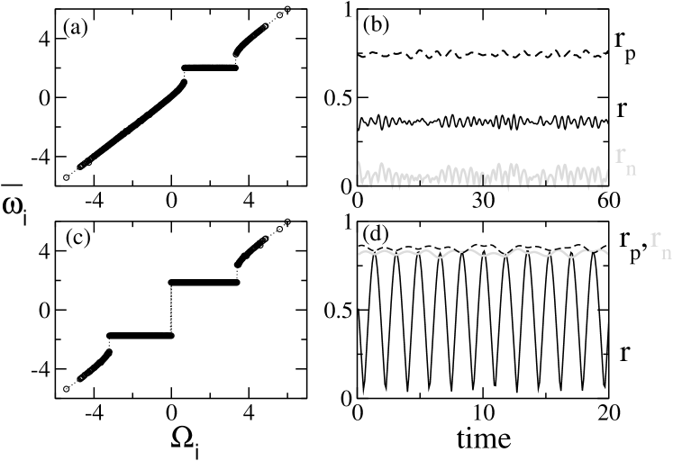
Figure 5: Bimodal frequency distributions. Average phase velocity $\bar{\omega_{i}}$ of the rotators versus their natural frequencies $\Omega_{i}$ for coupling strength K=6.2 (a) and K=6.8 (c). Panels (b) and (d) display the order parameter $r(t)$ (black line) versus time for the same coupling constants as in (a) and (c), respectively. The dashed black (continuous grey) line denotes the time evolution of $r_{p}$ ($r_{n}$). For each simulation an initial transient time $T_{R}=1000$ has been discarded and the average are estimated over a time interval $T_{W}=200$. In both cases $m=2$, $N=2000$ and $\Omega_{0}=2$.

The SWs are observable at larger coupling constants, this is characterized by two symmetrical clusters with opposite average velocities $\simeq\pm\Omega_{0}$, as shown in Fig. 5 (c). The presence of these two clusters now induces clear periodic oscillations in the order parameter $r(t)$, as observable in Fig. 5 (d). The period of the oscillations is related to $|\Omega_{0}|$, i.e. the average frequency of the clustered oscillators. However, at variance with the results reported in Fig. 3 (b) for the unimodal distribution the two symmetric clusters do not coexist with a cluster of locked oscillators with zero average velocity. By examining separately $r_{p}$ and $r_{n}$ reported in Fig. 3 (d), we notice that each sub-population is much more synchronized than the global one, in fact $r_{p}$ and $r_{n}$ have a higher average value than $r$ with superimposed irregular oscillations.

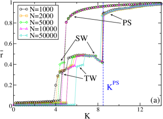
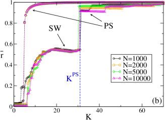
Figure 6: Bimodal frequency distribution with $\Omega_{0}=2$. Average order parameter ${\bar{r}}$ versus $K$ for various system sizes $N$: (a) $m=1$, (b) $m=6$. The numerical data have been obtained by following protocol (I) and then protocol (II) from $K=0$ up to $K_{M}=20$ ($K_{M}=200$) for inertia m=1 (m=6) with $\Delta K=0.2$ ($\Delta K=0.5$). The vertical dashed blue line refers to $K^{PS}$. The average has been performed over a time window $T_{W}=200$, after discarding a transient time $T_{R}=5,000-50,000$ depending on the system size; the larger $T_{R}$ have been employed for the larger N.

The data reported so far refer to a single system size, however finite size effects are quite relevant for this model, as shown in [18] for unimodal distributions. In Fig.  6 (a) we report the synchronization transition for several system sizes, namely $1,000\leq N\leq 50,000$ for a small inertia value ($m=1$). We observe that $K^{TW}$ and $K^{SW}$ increase with the size $N$; in particular, the incoherent state is observable on a wider coupling interval by increasing $N$ (similarly to what reported in [18] for unimodal distributions). Finite size fluctuations induce transitions from the incoherent branch to the TW branch and from this to the SW branch. The fact that we do not observe transition back to the original states indicates that the energy barriers are higher from these sides. A quite astonishing result is the fact that the transition value $K^{PS}$ and $K^{DS}$ seem completely independent from $N$. The combination of these results seem to suggest that in the thermodynamic limit the incoherent state will loose stability at $K^{PS}$ and therefore the two branches corresponding to TW and SW will be no more visited, at least by following protocol (I).

By observing all the data reported in Fig.  6 (a) for various $N$ and for protocol (I) and (II), it seems that there are clear indications that the two branches of solutions, corresponding to TW and SW, emerge via a supercritical bifurcation at the same coupling, namely $K\simeq 3.8$, while the transition to PS is clearly subcritical. These results confirm the analysis reported in [1] for a system with noise (in particular, see Fig. 17 in that paper). However, Acebrón et al. affirm that the SW is stable, while the TW is unstable. From our results, both branches seem to become inaccessible (in absence of noise) from the incoherent state, while at least a part of these branches appear to be reachable from the PS state by decreasing $K$ below $K^{DS}$ following protocol (II). Another important difference with respect to the results reported in [1] is that the PS regime is clearly hysteretic revealing two coexisting branches of PS states visited by following protocol (I) or (II).

As shown in Fig. 6 (b), for larger inertia (namely, $m=6$), the transition from the incoherent state following protocol (I) occurs via the emergence of many small clusters leading finally to a SW state. In this case the critical value at which the incoherent state looses stability seems to saturate to a constant value already for $N\geq 2,000$. The value of $K^{PS}$ is also in this case insensible to the system size. For large inertia values, the TWs seem no more observable.

As a further aspect, we will report the numerical results of the dependence on the inertia of the critical coupling constant $K^{PS}$, while the value of $K^{DS}\simeq 4.9$ is independent not only by $N$, but also by the inertia. As shown in Fig. 7, $K^{PS}$ increases linearly with the inertia and this scaling is already valid for not too large inertia values. The linear scaling with the inertia is analogous to the scaling recently found within a theoretical mean-field analysis for the coupling $K_{1}^{MF}$, which delimits the range of linear stability of the asynchronous state [1, 10]. In particular, the authors in [18] have shown for a Gaussian unimodal distribution of width $\sigma$ that $K_{1}^{MF}\simeq 2\sigma(0.64+m\sigma)$, which shows a linear dependence on the inertia and a quadratic dependence on the variance of the frequency distribution.

Figure 7: Critical value $K^{PS}$ as a function of the inertia. The dashed line represents the fit of the numerical data and indicates a linear increasing of $K^{PS}$ as a function of the inertia being the fit $K^{PS}=4(1.245+1.0525m)$. For all cases $N=2000$, $\Omega_{0}=2$. The data have been obtained by employing protocol (I) and for each simulation an initial transient time $T_{R}=5000$ has been discarded and data are averaged over a time $T_{W}=200$.

In the final part of this sub-section we perform an analysis analogous to that reported in Sub-Sect. 1.3.3, in particular starting from states with a finite level of synchronization obtained by following protocol (I) we decrease the coupling and observe how these states evolve. In Fig.  8, we report the results of these simulations (shown as empty triangles) for two different inertia values, namely $m=1$ and $m=10$. Starting from PS states we observe that the cluster survives until the descending curve obtained with protocol (II) is encountered, analogously to the results reported in Fig. 3 for the unimodal distribution. Therefore any part of the hysteretic portion of the $(K,r)$-plane delimited by the PS curves obtained via protocol (I) or (II) is accessible . However, if one starts for $m=1$ from a TW or a SW state, one observes only two curves (corresponding to the TW and SW branches previously discussed) which seem to end up at the same critical coupling which is smaller than $K^{DS}$. Therefore it seems that there are no evidences of hysteresis for this small inertia for SW and TW solutions (as shown in Fig.  8 (a)). For large inertia values $m=10$, since now, apart the SW solutions, there are solutions with many small clusters, the situations is much more complex. By starting from different values of $K<K^{PS}$ and by decreasing $K$, these curves seem all to end up at the same critical coupling smaller $K^{PS}$, see Fig.  8 (b). These results suggest that for large inertia values is possible to observe a continuum of possible states even starting from states characterized by (many) drifting clusters and that these states coexist in a wide range of coupling.

Figure 8: Bimodal frequency distribution. Average order parameter ${\bar{r}}$ versus the coupling constant $K$ for $m=1$ and $N=10,000$ (panel (a)) and for $m=10$ and $N=2,000$ (panel (b)). The filled circles have been obtained by following protocol (I) and then (II) starting from $K=0$ until $K_{M}=20$ ($K_{M}=100$) with steps $\Delta K=0.2$ ($\Delta K=0.5$); the empty triangles refer to simulations performed by starting from a final configuration obtained during protocol (I) and by decreasing the coupling from such initial configurations. The numerical data refer to $\Omega_{0}=2$, $T_{R}=50000$ ($T_{R}=5000$), and $T_{W}=2000$.

0.4.2 Overlapping Gaussians

In this sub-section, we analyze a bimodal distribution, where the two Gaussians are largely overlapping, since $\Omega_{0}=0.2$. In this case we expect to observe a phenomenology of the synchronization transition quite similar to the one seen for the unimodal case. In Fig. 9(a) is reported the average order parameter ${\bar{r}}$ versus the coupling constant $K$ estimated by following protocol (I) and (II) for various inertia values and for a fixed system size, namely $N=10,000$. We observe that all the curves obtained for protocol (II) almost overlap irrespectively of the used inertia, while the protocol (I) curves reveal a strong dependence on $m$. In particular, the hysteretic region widens with $m$. For small inertia values, namely $m=1$ and 2, there is a sudden transition from the asynchronous state to a PS state at $K^{PS}$ and neither traveling waves nor standing waves are observable: a single cluster at zero velocity emerges in correspondence of $K^{PS}$ and the order parameter never shows oscillating behavior in time.

For $m=6$, it is possible to observe a scenario similar to the one reported in Fig. 3 (b), where not only a cluster at zero velocity is present, but also two symmetrical clusters at finite velocities emerge. In particular, following protocol (I) for $K>2.4$ a small cluster of locked oscillators emerges; at larger coupling, namely $K\geq 3$, two symmetrical clusters of whirling oscillators emerge and coexist with the zero velocity cluster. Finally, at $K=10.8$ the PS regime arises, corresponding to a single large cluster of locked oscillators. Furthermore, in the range $3\leq K<10.8$ the order parameter reveals irregular oscillations. A more detailed analysis is needed to understand the origin of these oscillations as done in the next Section.

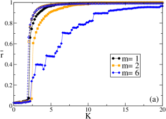
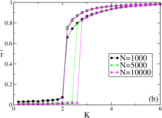
Figure 9: Bimodal frequency distribution for $\Omega_{0}=0.2$. Panel (a) : Average order parameter ${\bar{r}}$ versus $K$ for various inertia values and N=1000. The numerical data have been obtained by following protocol (I) and then protocol (II) from $K=0$ up to $K_{M}=20$ for all inertia values with $\Delta K=0.2$ . Panel (b): Average order parameter ${\bar{r}}$ versus the coupling constant $K$ for various system sizes N and m=1. Data have been obtained by averaging the order parameter over a time window $T_{W}=200$, after discarding a transient time $T_{R}=5,000-50,000$ depending on the system size.

Finally, we examine the influence of the system size on the studied transitions: for $m=1$ the results for the protocol (I) [protocol (II)] simulations are reported in Fig. 9(b) for sizes ranging from $N=1,000$ to $N=10,000$. It is immediately evident that the transition from synchronized state to the asynchronous state, following protocol (II), does not depend on N: for all considered sizes the transition happens in correspondence of $K\simeq 2$, analogously to what reported for unimodal distributions [18]. Starting from the incoherent regime and following protocol (I) the system reveals a jump to a finite $\bar{r}$ value for critical couplings increasing with $N$, quite similar once more to the results reported for unimodal distributions. We can conclude this sub-section by affirming that the phenomenology seen for bimodal, but largely overlapping, distributions should not differ much from the one observed for unimodal distributions.

0.5 Linear Stability Analysis

To better characterize the synchronization transitions and the stability of the observed states it is worth estimating the maximal Lyapunov exponent $\lambda_{M}$ following protocol (I) and (II) for an unimodal and a bimodal distributions. This quite time consuming analysis has been performed for a single inertia value $m=6$ and a single system size $N=1,000$, the scaling of $\lambda_{M}$ with $N$ will be discussed in the following for specific coupling constant values.

In general, we observe that once the system fully synchronizes, $\lambda_{M}$ vanishes; therefore for most of the simulations associated to protocol (II) corresponding to fully synchronized cluster down to the desynchronization transition, $\lambda_{M}$ is zero. This is not the case for protocol (I) simulations which reveal a positive $\lambda_{M}$ as soon as $\bar{r}$ is non zero. Thus indicating that not only the dynamics characterized in terms of the macroscopic order parameter $\bar{r}$ is hysteretic, but also at the level of the microscopic dynamics, investigated via $\lambda_{M}$, the system has a clear hysteretic behavior.

The behavior of $\lambda_{M}$ with $K$ exhibits chaotic dynamical states with windows of regularity for both unimodal and bimodal distribution with $\Omega=2$, as shown in Figs. 10 (a) and (b). As a general aspect, we observe the maximal level of chaoticity immediately after the transition from the incoherent state to partially coherence, where small clusters of synchronized oscillators and drifting oscillators coexist. The increase of $\bar{r}$ is accompanied by a trend of $\lambda_{M}$ to decrease and finally to vanish for $\bar{r}\to 1$

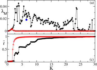
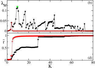
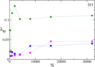
Figure 10: Maximal Lyapunov exponent $\lambda_{M}$ and the average order parameter ${\bar{r}}$ versus $K$ for unimodal (bimodal with $\Omega_{0}=2$) are shown in panel (a) (panel (b)) and in panel (c) (panel (d)), respectively. The numerical data have been obtained by following protocol (I) (black circles) and then protocol (II) (red diamonds) from $K=0$ up to $K_{M}=30$ ($K_{M}=80$) with $\Delta K=0.2$ ($\Delta K=0.8$). For panels (a),(c) $T_{R}=500$, and $T_{W}=50,000$; for panels (b),(d) $T_{R}=500$, and $T_{W}=400000$. The different symbols in (a) and (b) denote the value for which the further analysis reported in panel (e) has been done. Panel (e): $\lambda_{M}$ versus $N$ for different couplings and frequency distributions. Blue circles refer to unimodal distribution and coupling constant $K=6.5$; magenta squares (green diamonds) refer to binomial distributions with $\Omega_{0}=0.2$ and $K=6.7$ ($\Omega_{0}=2$ and $K=9.5$). $\lambda_{M}$ has been averaged over a time window $T_{W}=4,000-400,000$, after discarding a transient time $T_{R}=1,000-10,000$ depending on the system size. For all panels $m=6$ and $N=1,000$.

An important aspect to understand is if this dynamics is weakly chaotic or not, in particular this amounts to verify if, in the thermodynamic limit, $\lambda_{M}$ will vanish or will remain finite. In order to test for this aspect, we have considered a configuration obtained by following protocol (I) for a specific coupling and analyzed $\lambda_{M}$ versus the system size for $200\leq N\leq 32,000$. The results for unimodal distributions, as well as for bimodal ones with $\Omega_{0}=2$ and $\Omega_{0}=0.2$ are shown in Fig. 10 (e). It is clear for all the considered cases that the system remains chaotic for diverging system sizes.

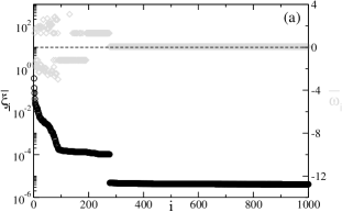
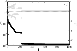
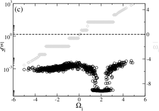
Figure 11: Average squared amplitude of the components of the maximal Lyapunov vector $\bar{\xi}_{i}$ (black circles) and average frequencies $\bar{\omega}_{i}$ (grey diamonds) versus the rotator index for unimodal (a) and bimodal distribution with $\Omega_{0}=0.2$ (b). In both panels the oscillators are ordered according to the values of $\bar{\xi}_{i}$. Panel (c): $\bar{\xi}_{i}$ (black circles) and average frequencies $\bar{\omega}_{i}$ (grey diamonds) of the oscillators as a function of their natural frequency for bimodal distribution with $\Omega_{0}=2$. Panel (a) refers to coupling constant $K=6.5$, panel (b) to $K=6.7$ and panel (c) to $K=9.5$. For all panels inertia $m=6$ and $N=1,000$, $T_{R}=500$, and $T_{W}=400000$.

As a final aspect we would like to understand which oscillators contribute more to the chaotic dynamics of the system; this can be understood by measuring the average squared amplitude of the components of the maximal Lyapunov vector  $\bar{\xi}_{i}$ (see the definition reported in Eq. 4). In particular, we consider the three cases analyzed in Fig. 10 (e) for $N=1,000$. The corresponding results are shown in Fig. 11. From panel (a) and (b) of the figure it is clear that for the unimodal distribution, as well as for the largely overlapping bimodal distributions, the chaotic activity is associated almost exclusively to the rotators which are outside the large clusters of locked oscillators with $\bar{\omega}_{i}\simeq 0$. Thus confirming recent results reported for two coupled populations of rotators with identical natural frequencies [17].

However, the situation for the bimodal distribution with $\Omega_{0}=2$ is different; in particular, as shown in Fig. 11 (c), the network for this large value of the inertia and the considered coupling does not exhibit a cluster of locked oscillators with $\bar{\omega}_{i}\simeq 0$, but only drifting clusters. In this case the rotators outside and inside the clusters seem to contribute equally to the maximal Lyapunov vector, with the possible exclusion of a group of rotators with $\Omega_{i}\simeq\Omega_{0}$.

0.6 Conclusions

We have studied the synchronization transition for a globally coupled Kuramoto model with inertia for different frequency distributions. For the unimodal frequency distribution we have shown that clusters of locked oscillators of any size coexist within the hysteretic region. This region is delimited by two curves in the plane individuated by the coupling and the average value of the order parameter. Each curve corresponds to the synchronization (desynchronization) profile obtained starting from the fully desynchronized (synchronized) state. For sufficiently large inertia values, clusters composed by drifting oscillators with opposite velocities (standing wave state) emerge in addition to the locked oscillators clusters. The presence of clusters of whirling rotators induces oscillatory behavior in the order parameter.

For bimodal frequency distribution the scenario can become more complex since it is possible to play with an extra parameter: the distance between the peaks of the distributions. For simplicity we have analyzed only two cases: largely overlapping distributions ($\Omega_{0}=0.2$), and almost not overlapping distributions ($\Omega_{0}=2$). The phenomenology observed for $\Omega_{0}=0.2$ resembles strongly that found for the unimodal distribution. The analysis of the non overlapping case reveals new interesting features. In particular, the transition from incoherence to coherence occurs via several states: namely, traveling waves, standing waves and finally partial synchronization. This scenario resembles that reported for the usual Kuramoto model for a bimodal distribution  [5, 15, 19]. However, in our case the transition is always largely hysteretic, and for non overlapping distributions, traveling waves are clearly observable at variance, not only with the results for the Kuramoto model  [5, 15, 19], but also with the theoretical phase diagram reported in [1] for oscillators with inertia. A peculiar aspect is that in the thermodynamic limit we expect a direct discontinuous jump from the incoherent to the coherent phase, without passing through any intermediate state. The critical coupling $K^{PS}$ required to pass from incoherence to partial synchronization is independent of the system size and grows linearly with inertia, while the partially synchronized state looses its stability at a smaller coupling $K^{DS}<K^{PS}$ which is the same for any inertia value and system size.

Finally, by performing a linear stability analysis we have been able to show that the hysteretic behavior is not limited to macroscopic observables, as the level of synchronization, but it is revealed also by microscopic indicators as the maximal Lyapunov exponent. In particular, we expect that in a large interval of coupling values chaotic and non chaotic states will coexist.

References

- [1] J. Acebrón, L. Bonilla, and R. Spigler. Synchronization in populations of globally coupled oscillators with inertial effects. Physical Review E, 62(3):3437, 2000.
- [2] J. Acebrón and R. Spigler. Adaptive frequency model for phase-frequency synchronization in large populations of globally coupled nonlinear oscillators. Physical Review Letters, 81(11):2229, 1998.
- [3] G. Benettin, L. Galgani, A. Giorgilli, and J.-M. Strelcyn. Lyapunov characteristic exponents for smooth dynamical systems and for hamiltonian systems; a method for computing all of them. part 1: Theory. Meccanica, 15(1):9–20, 1980.
- [4] M. Bennett, M. F. Schatz, H. Rockwood, and K. Wiesenfeld. Huygens’s clocks. Proceedings: Mathematics, Physical and Engineering Sciences, pages 563–579, 2002.
- [5] J. D. Crawford. Amplitude expansions for instabilities in populations of globally-coupled oscillators. Journal of statistical physics, 74(5-6):1047–1084, 1994.
- [6] F. Dörfler, M. Chertkov, and F. Bullo. Synchronization in complex oscillator networks and smart grids. Proceedings of the National Academy of Sciences, 110(6):2005–2010, 2013.
- [7] B. Ermentrout. An adaptive model for synchrony in the firefly pteroptyx malaccae. Journal of Mathematical Biology, 29(6):571–585, 1991.
- [8] G. Filatrella, A. H. Nielsen, and N. F. Pedersen. Analysis of a power grid using a kuramoto-like model. The European Physical Journal B, 61(4):485–491, 2008.
- [9] F. Ginelli, K. A. Takeuchi, H. Chaté, A. Politi, and A. Torcini. Chaos in the hamiltonian mean-field model. Physical Review E, 84(6):066211, 2011.
- [10] S. Gupta, A. Campa, and S. Ruffo. Nonequilibrium first-order phase transition in coupled oscillator systems with inertia and noise. Physical Review E, 89(2):022123, 2014.
- [11] P. Jaros, Y. Maistrenko, and T. Kapitaniak. Chimera states on the route from coherence to rotating waves. Physical Review E, 91(2):022907, 2015.
- [12] P. Ji, T. K. D. Peron, P. J. Menck, F. A. Rodrigues, and J. Kurths. Cluster explosive synchronization in complex networks. Phys. Rev. Lett., 110:218701, May 2013.
- [13] D. J. Jörg. Nonlinear transient waves in coupled phase oscillators with inertia. Chaos: An Interdisciplinary Journal of Nonlinear Science, 25(5):053106, 2015.
- [14] Y. Kuramoto. Chemical oscillations, waves, and turbulence. Courier Dover Publications, 2003.
- [15] E. A. Martens, E. Barreto, S. Strogatz, E. Ott, P. So, and T. Antonsen. Exact results for the kuramoto model with a bimodal frequency distribution. Physical Review E, 79(2):026204, 2009.
- [16] T. Nishikawa and A. E. Motter. Comparative analysis of existing models for power-grid synchronization. New Journal of Physics, 17(1):015012, 2015.
- [17] S. Olmi, E. A. Martens, S. Thutupalli, and A. Torcini. Intermittent chaotic chimeras for coupled rotators. arXiv:1507.07685, 2015.
- [18] S. Olmi, A. Navas, S. Boccaletti, and A. Torcini. Hysteretic transitions in the kuramoto model with inertia. Physical Review E, 90(4):042905, 2014.
- [19] D. Pazó and E. Montbrió. Existence of hysteresis in the kuramoto model with bimodal frequency distributions. Physical Review E, 80(4):046215, 2009.
- [20] M. Rohden, A. Sorge, M. Timme, and D. Witthaut. Self-organized synchronization in decentralized power grids. Physical review letters, 109(6):064101, 2012.
- [21] F. Salam, J. E. Marsden, and P. P. Varaiya. Arnold diffusion in the swing equations of a power system. Circuits and Systems, IEEE Transactions on, 31(8):673–688, 1984.
- [22] S. H. Strogatz. Nonlinear dynamics and chaos (with applications to physics, biology, chemistry a. Perseus Publishing, 2006.
- [23] S. H. Strogatz, D. M. Abrams, A. McRobie, B. Eckhardt, and E. Ott. Theoretical mechanics: Crowd synchrony on the millennium bridge. Nature, 438(7064):43–44, 2005.
- [24] H.-A. Tanaka, A. J. Lichtenberg, and S. Oishi. First order phase transition resulting from finite inertia in coupled oscillator systems. Physical review letters, 78(11):2104, 1997.
- [25] H.-A. Tanaka, A. J. Lichtenberg, and S. Oishi. Self-synchronization of coupled oscillators with hysteretic responses. Physica D: Nonlinear Phenomena, 100(3):279–300, 1997.
- [26] B. Trees, V. Saranathan, and D. Stroud. Synchronization in disordered josephson junction arrays: Small-world connections and the kuramoto model. Physical Review E, 71(1):016215, 2005.
- [27] A. Winfree. The Geometry of Biological Time. Springer-Verlag, Berlin-Heidelberg-New York, 1980.
Index
- bimodal frequency distribution §0.1, §0.4
- collective dynamics §0.3.3, §0.4.1
- drifting oscillators §0.3.3
- finite size effects §0.4.1
- full synchrony §0.4.1
- hysteresis §0.4.1
- hysteretic transition §0.3.1, §0.3.2
- inertia §0.1, §0.3.2, §0.4
- Kuramoto model with inertia §0.1, §0.2, §0.2
- linear stability analysis §0.5
- locked oscillators §0.3.3, §0.4.1
- Lyapunov vector §0.5
- maximal Lyapunov exponent §0.2.1, §0.5
- mean field theory §0.3.2
- partial synchronization §0.1, §0.4.1
- phase oscillator §0.1
- power grids §0.1
- rotators §0.1
- standing waves §0.1, §0.3.3, §0.4.1
- synchronization §0.2
- synchronization order parameter §0.2
- synchronization transition §0.1, §0.3.1
- traveling waves §0.1, §0.4.1
- unimodal frequency distribution §0.3