The early phases of the type Iax supernova SN 2011ay

Abstract

We present a detailed study of the early phases of the peculiar supernova 2011ay based on BVRI photometry obtained at Konkoly Observatory, Hungary, and optical spectra taken with the Hobby-Eberly Telescope at McDonald Observatory, Texas. The spectral analysis carried out with SYN++ and SYNAPPS confirms that SN 2011ay belongs to the recently defined class of SNe Iax, which is also supported by the properties of its light and color curves. The estimated photospheric temperature around maximum light, $T_{phot}\sim$ 8,000 K, is lower than in most Type Ia SNe, which results in the appearance of strong Fe II features in the spectra of SN 2011ay, even during the early phases. We also show that strong blending with metal features (those of Ti II, Fe II, Co II) makes the direct analysis of the broad spectral features very difficult, and this may be true for all SNe Iax. We find two alternative spectrum models that both describe the observed spectra adequately, but their photospheric velocities differ by at least $\sim 3,000$ km s^-1. The quasi-bolometric light curve of SN 2011ay has been assembled by integrating the UV-optical spectral energy distributions. Fitting a modified Arnett-model to $L_{bol}(t)$, the moment of explosion and other physical parameters, i.e. the rise time to maximum, the ⁵⁶Ni mass and the total ejecta mass are estimated as $t_{rise}\sim$14$\pm$1 days, $M_{Ni}\sim$0.22$\pm$0.01 $M_{\odot}$ and $M_{ej}\sim$ 0.8 $M_{\odot}$, respectively.

1 Introduction

Type Iax supernovae (SNe Iax), previously labeled as SN 2002cx-like ones, are spectroscopically similar to SNe Ia, but thought to have lower velocities at maximum light and lower peak magnitudes (Foley et al., 2013). There are 25 members of this class known to date, but it is suggested that in a given volume there may be 30-40 SNe Iax for every 100 SNe Ia.

The major question about SNe Iax is the nature of their progenitors. The similarity of their light curves to those of “normal” SNe Ia (especially their rise times), their spectral features, and the lack of X-ray and radio detections suggest that they originate from compact progenitors, probably white dwarfs (WDs). At the same time, explosions causing the total disruption of WDs (either via detonation or via pure deflagration) are not in agreement with the observational results. This statement was recently strengthened by McCully et al. (2014a) who analyzed late-time spectra of two SNe Iax.

Partial disruption of WDs seems to be a feasible model to explain the properties of this new class of stellar explosions (Foley et al., 2013; McCully et al., 2014a). This model seems to give a plausible explanation for the diversity of this class (including extremely faint and low-velocity explosions, like SN 2008ha). It is also supported by recently published results of numerical 3D simulations (Jordan et al., 2012; Krömer et al., 2013). As Foley et al. (2013) and Wang, Justham & Han (2013) proposed, WDs accreting material from their helium-star companion in binary systems may be good candidates for the progenitors of SNe Iax. This assumption has been recently strengthened by the detection of the luminuous, blue progenitor system of the type Iax SN 2012Z (McCully et al., 2014b). At the same time, the observed properties of this object, and maybe those of other SNe Iax, can be also explained with the pulsational delayed detonation of a single WD (see Stritzinger et al., 2015, and references therein).

Other ideas, e.g. the theory of the “.Ia” events (which are thought to be luminous helium shell flashes of WDs in binary systems with low accretion rates, Bildsten, 2007), do not seem to give self-consistent description of the observations (Foley et al., 2009, 2013). Note, however, that the .Ia models might be good alternatives to explain the extremely low-luminosity events, like SN 2008ha.

On the other hand, so far almost all SNe Iax have been found in late-type galaxies with recent, strong star formation activity (Lyman et al., 2013; Foley et al., 2013). This fact might lead to the suspicion that SNe Iax actually could be low-luminosity core-collapse (CC) events emerging from 7-9 M_⊙, stripped-envelope stars (Valenti et al., 2009; Lyman et al., 2013), even though the observed properties of SNe Iax are more similar to those of Ia than CC SNe. In this scenario the explosion might not have enough energy to eject the entire stellar envelope, thus, part of the ejecta falls back to the central remnant (Valenti et al., 2009; Moriya et al., 2010). Note, however, that SN 2008ge, another SN Iax, is situated in a region that has no detectable star-formation, thus, there are probably no massive stars near the SN site (Foley et al., 2010b, 2013).

To understand the general properties of SNe Iax, it is important to study single, well-observed objects as thoroughly as possible. Up to now, detailed photometric and spectroscopic analyses have been published only on a few of them: SN 2002cx (Li et al., 2003; Branch et al., 2004; Jha et al., 2006), SN 2005hk (Chornock et al., 2006; Phillips et al., 2007; Sahu et al., 2008; McCully et al., 2014a), SN 2007qd (McClelland et al., 2010), SN 2008A (McCully et al., 2014a), SN 2008ge (Foley et al., 2010b), SN 2008ha (Foley et al., 2009; Valenti et al., 2009; Foley et al., 2010a), SN 2009ku (Narayan et al., 2011), SN 2010ae (Stritzinger et al., 2014), SN 2012Z (McCully et al., 2014b; Stritzinger et al., 2015; Yamanaka et al., 2015), and SN 2014dt (Foley et al., 2015). Moreover, Foley et al. (2013) presented light curves and spectra of some other SNe Iax for which detailed studies are in progress.

Here we present a detailed analysis of SN 2011ay, another SN Iax. This object was discovered on March 18.18 UT by the KAIT/LOSS program with an apparent, unfiltered brightness of 17.7 mag (Blanchard et al., 2011). The SN located 9.3″east and 1.4″south from the center of NGC 2315. The average Hubble-flow distance of the host galaxy is 86.9$\pm$6.9 Mpc, as listed in the NASA/IPAC Extragalactic Database (NED). Based on a quick analysis of an early spectrum, Pogge, Garnavich & Pedani (2011) classified SN 2011ay as a peculiar Ia, while Silverman et al. (2011) reported that it may belong to the SN 2002cx-like events. Foley et al. (2013) confirmed the classification and also published some optical photometry and spectra of this object.

Our motivation was to carry out a detailed analysis using data obtained during the early photospheric phase of the SN. We present our simultaneous photometric and spectroscopic observations in Section 2, while the light and color curves, the UV-optical spectral energy distributions (SEDs) and the results of modeling the spectra and the light curve are shown in Section 3. In Section 4 we discuss our results and present our conclusions.

2 Observations and data reduction

2.1 Photometry

Ground-based photometric observations for SN 2011ay were obtained from the Piszkéstető Mountain Station of Konkoly Observatory, Hungary. We used the 0.6/0.9 m Schmidt-telescope and the 1.0m RCC-telescope, both equipped with Bessell BVRI filters. Figure 1 shows a BVI composite image of the SN and its host galaxy.

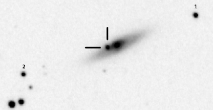
Figure 1: BVI composite image of the SN 2011ay and its host galaxy on 2011 March 24 (0.6/0.9 m Schmidt-telescope, Konkoly Observatory, Hungary). The numbered objects were used as local comparison stars.

We used the daophot/allstar task in IRAF to carry out PSF-photometry on the SN and two nearby comparison stars (see Figure 1). Because the SN appeared close to the center of the nearly edge-on host galaxy, the value of background flux level was estimated interactively in every case. The background level estimates produced by the fitskypars task were adjusted by eye and the background was subtracted manually for each frame.

The instrumental magnitudes were transformed to the standard system applying the following equations:

$$V-v=C_{V}\cdot(V-I)+\zeta_{V}$$

$$(B-V)=C_{BV}\cdot(b-v)+\zeta_{BV}$$

$$(V-R)=C_{VR}\cdot(v-r)+\zeta_{VR}$$

$$(V-I)=C_{VI}\cdot(v-i)+\zeta_{VI},$$ (1)

where lowercase and uppercase letters denote instrumental and standard magnitudes, respectively. The color terms ($C_{X}$), determined by measuring Landolt standard stars during photometric conditions close to the epochs of the SN observations, were the followings: C_V = $−$0.047, C_BV = 1.228, C_VR = 0.960, C_VI = 0.934. Because simultaneous observation of the Landolt field and the SN field was not possible, we applied Eq. (1) to the differential magnitudes $\Delta m=m_{SN}-m_{C1,2}$ constructed from the instrumental magnitudes of the SN and the comparison stars, thus, eliminating the zero points ($\zeta_{X}$). Then, using the standard BVRI magnitudes of the comparison stars calculated from their SDSS-magnitudes (based on the calibration of Jordi, Grebel & Ammon, 2006), the standard magnitudes of SN 2011ay were obtained in the Johnson-Cousins system. The results are presented in Table 1. Errors (given in parentheses) contain both the uncertainties of the PSF-photometry and the standard transformation.

The optical data were supplemented by the available Swift/UVOT data (reduced using standard HEAsoft tasks). Individual frames were summed with the uvotimsum task, and magnitudes were determined via aperture photometry using the task uvotsource. The object could be roughly separated from the galactic nucleus only in channels b, u, and uw1, while it got too faint after $\sim$2 weeks. The results of Swift-photometry are shown in Table 2.

Table 1: BVRI magnitudes of SN 2011ay from the Konkoly Observatory, Hungary

JDa	B (mag)	V (mag)	R (mag)	I (mag)
5645.3	16.89(.07)	16.97(.05)	16.75(.06)	16.74(.10)
5647.3	16.85(.02)	16.71(.05)	16.52(.06)	16.33(.08)
5649.3	16.99(.03)	16.62(.07)	16.44(.06)	16.31(.08)
5650.3	16.99(.06)	16.54(.04)	16.50(.05)	16.28(.08)
5651.3	16.97(.05)	16.65(.07)	16.42(.06)	16.21(.07)
5655.3	17.30(.06)	16.62(.07)	16.31(.06)	16.10(.07)
5657.3	17.38(.07)	16.63(.06)	16.28(.06)	16.09(.07)
5661.6	18.02(.15)	16.86(.06)	16.36(.05)	16.21(.07)
5669.3	18.82(.23)	17.71(.03)	16.88(.04)	16.43(.02)
5671.3	19.05(.12)	17.78(.09)	17.05(.03)	16.48(.02)

Notes. ^(a)JD$-$2,450,000. Errors are given in parentheses.

Table 2: Swift magnitudes of SN 2011ay

JDa	UVW1 (mag)	U (mag)	B (mag)
5645.5	17.70(.12)	16.53(.07)	16.59(.05)
5648.0	17.98(.11)	16.63(.07)	16.66(.05)
5650.1	18.22(.13)	16.75(.06)	16.67(.05)
5651.8	18.32(.14)	16.91(.08)	16.80(.05)
5653.5	18.17(.13)	17.14(.10)	16.79(.06)
5655.6	18.66(.25)	17.26(.12)	17.01(.08)
5657.6	18.73(.19)	17.36(.10)	17.18(.07)
5660.1	18.83(.22)	17.88(.18)	17.54(.11)

Notes. ^(a)JD$-$2,450,000. Errors are given in parentheses.

2.2 Spectroscopy

Optical spectra of SN 2011ay were obtained with the 9.2m Hobby-Eberly Telescope (HET) Marcario Low Resolution Spectrograph (LRS, Hill et al., 1998) at McDonald Observatory, Texas, between March 24 and April 19, 2011. LRS has a spectral coverage of 4,200–10,200 Å and a resolving power of $\lambda/\Delta\lambda\sim$ 600. The data were reduced with standard IRAF routines. Table 3 contains the journal of the spectroscopic observations, while the extracted, wavelength- and flux-calibrated spectra are collected in Figure 2.

Table 3: Log of spectral observations obtained with HET LRS

Date	JDa	Phaseb (d)	Exp. time (s)
2011-03-23	5643.2	$-$10	1500
2011-03-24	5644.2	$-$9	1800
2011-03-26	5646.2	$-$7	1500
2011-03-27	5647.2	$-$6	1500
2011-03-28	5648.2	$-$5	1500
2011-03-29	5649.2	$-$4	1500
2011-03-31	5651.2	$-$2	1500
2011-04-14	5665.1	+12	1500
2011-04-19	5670.1	+17	1500

Notes. ^(a)JD$-$2,450,000; ^(b) with respect to the moment of maximum light in V-band.

Figure 2: HET spectra of SN 2011ay. Epochs are given relative to V-band maximum. The spectra are shifted vertically for better visibility.

3 Data analysis and results

3.1 Light curves and colors

The light curves consisting of standard BVRI and Swift magnitudes are shown in Figure 3. The Konkoly B and V curves are generally consistent with the ones published by Foley et al. (2013), but the sampling of our data around maximum is better (at longer wavelengths they observed SN 20011ay with $r$ and $i$ filters). As seen in Fig. 3, the data by Foley et al. (2013) do not provide new information in addition to our photometry during the early phases. While they followed the SN longer, their late-time photometry is much more uncertain, probably due to the increasing contribution from the host galaxy background flux. Thus, for further analysis we used only our data, but note that the results are consistent with the photometry by Foley et al. (2013).

By fitting low-order polynomials to the data around the maxima, the light-curve parameters could be determined with relatively low uncertainties. These parameters are listed in Table 4. Note that for normal SNe Ia the moment of B maximum is usually used as a reference epoch. Instead, we used the time of V maximum, which is closer to the moment of maximum luminosity, to be consistent with the analysis presented by Foley et al. (2013).

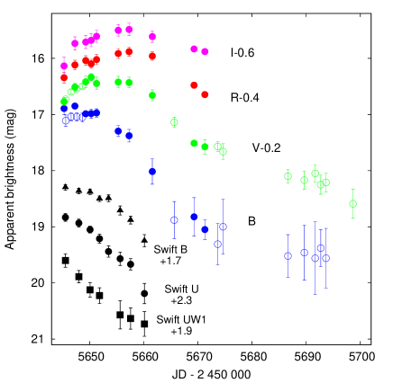
Figure 3: Standard BVRI (Konkoly Observatory) and Swift light curves of SN 2011ay (not corrected for reddening). The open circles denote the B and V data from Foley et al. (2013).

Table 4: Light-curve parameters of SN 2011ay

	B	V	R	I
$t_{max}$
(JD-2,450,000)	5646.6(1.1)	5653.6(0.4)	5657.2(1.1)	5656.2(0.8)
Peak mag.	16.89(.08)	16.56(.08)	16.30( .07)	16.08(.08)
Peak abs. mag.	$-$18.15(.17)	$-$18.39(.18)	$-$18.60(.17)	$-$18.76(.18)
$\Delta m_{15}$ (mag)	1.11(.16)	0.95(.08)	0.82(.07)	0.40(.08)

Notes. Errors are given in parentheses.

Figure 4: Color curves of SN 2011ay (corrected for Milky Way reddening, see the text for details). The values plotted with open circles were calculated using the B and V datapoints of Foley et al. (2013).

The color evolution of SN 2011ay (Figure 4) is very similar to other SNe Iax (see e.g. Li et al., 2003; Phillips et al., 2007; Foley et al., 2013): it gets redder after V-maximum until it reaches a nearly constant color at 15-20 days after maximum. Although the interstellar matter (ISM) in the host galaxy may contribute to the total reddening, it is probably low, because the SN appeared very blue, $(B-V)<0$ mag, at the earliest observed epochs. Thus, the color curves have been corrected only for Milky Way reddening, using $E(B-V)$ = 0.081 mag, $A_{V}$ = 0.23 mag, $A_{R}$ = 0.18 mag, and $A_{I}$ = 0.13 mag (Schlafly & Finkbeiner, 2011).

3.2 Spectroscopic analysis

In the following, we present detailed analysis of some of the HET spectra shown in Fig. 2 and Table 3. The $-9$d, $-2$d and $+17$d spectra were selected for this purpose, because they have the highest signal-to-noise and show the largest differences in their spectral features, i.e. the most noticeable evolution. Moreover, two additional spectra obtained by Foley et al. (2013) were also included in the sample of analyzed spectra. These two spectra were taken with the Lick/Kast spectrograph on April 2 and 5, 2011, at $0$d and $+3$d phases, respectively.

The application of the Supernova Identification (SNID) code (Blondin & Tonry, 2007) to the pre-maximum spectra of SN 2011ay revealed some similarity with spectra of normal Ic SNe. However, using SNID for the $+17$d HET spectrum we found that the relatively weak Si, dominating Fe II and strong Ca II features clearly imply that SN 2011ay most closely resembles SN 2005hk (see e.g. Sahu et al., 2008), i.e. it belongs to the Iax subclass, as first pointed out by Silverman et al. (2011) and Foley et al. (2013).

For more quantitative analysis, we applied the SYN++ and SYNAPPS codes (Thomas, Nugent & Meza, 2011), which are based on the original SYNOW code (Jeffery & Branch, 1990; Hatano et al., 1999), to model the selected spectra in order to reveal the chemical composition and other physical properties of the ejecta of SN 2011ay. SYNOW/SYN++/SYNAPPS assumes a fully opaque photosphere located at a specific velocity $v_{phot}$, where the electron-scattering optical depth $\tau_{es}=1$ (Hatano et al., 1999), in homologously expanding ejecta. The spectral features are assumed to be due to pure resonant scattering of the photons originating from the (assumed) blackbody emission of the photosphere. The scattering of photons take place in the partly transparent ejecta above the photosphere, where the strong velocity gradient (due to the rapid, homologous expansion) makes the scattering regions appear as thin planes perpendicular to the line of sight for each photon frequency/wavelength. This Sobolev-approximation, among others, is clearly a limitation for the applicability of such a code. Nevertheless, it was found to be surprisingly effective and useful for modeling P Cygni line profiles and identifying SN features (see e.g. Parrent, Friesen & Parthasarathy, 2014; Parrent, 2014).

Before the fitting, all spectra were corrected to Milky-Way extinction (adopting $E(B-V)=0.081$ mag as above) and the redshift of the host galaxy using $z$ = 0.021 (Miller & Owen, 2001).

Since parametrized models, like those from SYNAPPS/SYN++, depend heavily on the a-priori identification of ions and key parameters such as the velocity at the photosphere, we built two alternative models based on slightly different assumptions.

In the first model (hereafter Model A) all features were assumed as photospheric, i.e. the line formation region for all ions extends from the top of the ejecta, parametrized as a fixed $v_{max}$ = $40,000$ km s^-1 at all phases, down to the sharp edge of the photosphere, given as $v_{phot}$ in velocity coordinates. The density structure of the ions distributed within the line forming region is treated as a simple exponential, defined directly for the optical depth of a given feature as

$$\tau(v)~{}=~{}\tau(v_{ref})\times\exp[-(v-v_{ref})/v_{e}],$$ (2)

where $v_{ref}$ is a fixed reference velocity (arbitrary, but set close to $v_{phot}$) and $v_{e}$ is the e-folding width of the optical depth profile. SYN++ uses a quasi-LTE approximation for computing the relative strengths of the features for the same ion: the model specifies a single $\tau(v_{ref})$ optical depth for a pre-selected “reference” feature of the given atom/ion (see e.g. Hatano et al., 1999, for the list of reference lines for every ion), then the optical depths of all other same-ion features are computed assuming Boltzmann-excitation. The excitation temperature $T_{exc}$ can be set differently for every ion, mimicking a non-LTE-like excitation, although it is clearly very far from a true, self-consistent non-LTE treatment of the problem. Thus, in Model A, all features are assumed to be formed down to the photosphere, each ion can have a different excitation temperature ($T_{exc}$), a different reference line optical depth ($\tau(v_{ref})$) and different scale height of its line forming region ($v_{e}$).

The alternative model (hereafter Model B) was built by assuming two essential differences from Model A: instead of requiring that all features start to form at $v_{phot}$, the minimum velocity of their line-forming region, $v_{min}$, may be at higher velocities than $v_{phot}$. Such features, having $v_{min}>v_{phot}$, are called “detached” (Jeffery & Branch, 1990). This model may be more flexible than Model A, because $v_{min}$ can be different for every ion, but also less constrained, because the increasing number of parameters may decrease the uniqueness of the best-fit model. In addition, since $v_{phot}$ may become much less constrained in this model, we set the initial value of $v_{phot}$ at $\sim 6,000$ km s^-1 as estimated by Silverman et al. (2011) and Foley et al. (2013) for SN 2011ay particularly from the absorption minimum of the feature around $\sim 6200$ Å, which was thought to be due to Si II (but see Sect.3.3 for a discussion of this issue).

The chemical composition of both models was assembled based on the major features found in the spectra of other SNe Iax, namely 2002cx (Branch et al., 2004), 2005hk (Chornock et al., 2006; Sahu et al., 2008; McCully et al., 2014a), 2008A (McCully et al., 2014a), 2008ha and 2010ae (Stritzinger et al., 2014): O I, O II, Na I, Mg II, Si II, S II, Ca II, Ti II, Fe II, Fe III and Co II. Not all ions were detected in all spectra, e.g. the ones with higher ionization potential (O II and Fe III) were not found in the late-phase $+17$d spectrum.

For both models, the optimum set of parameters that give the best fit for the synthesized spectrum to the observed one were found automatically by SYNAPPS via $\chi^{2}$-minimization. The total number of the optimized parameters were $\sim 50$ in a typical run. Note that there is an essential degeneracy between $\tau(v_{ref})$, $v_{phot}$ (or $v_{min}$) and $v_{e}$ (Jeffery & Branch, 1990; Parrent, 2014), thus, their finally adopted values may not represent a unique solution for any spectra.

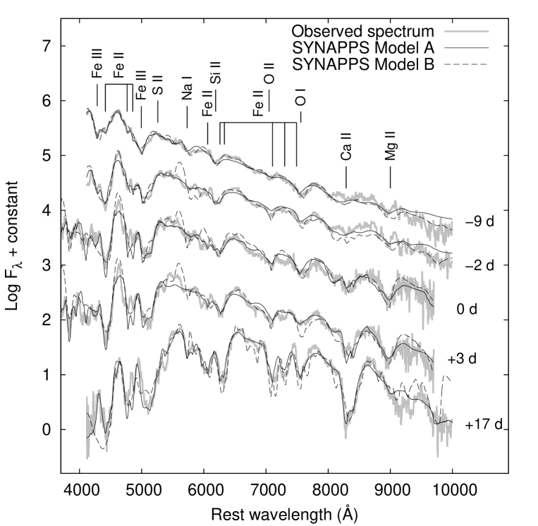
Figure 5: The best-fit SYNAPPS model spectra for Model A (solid line) and Model B (dashed line) plotted together with the observed spectra at $-9$d, $-2$d, $0$d, $+3$d and $+17$d phases. Strong blending makes feature identification ambiguous at all phases. Some of the strongest contributing ions are marked by vertical lines and labels.

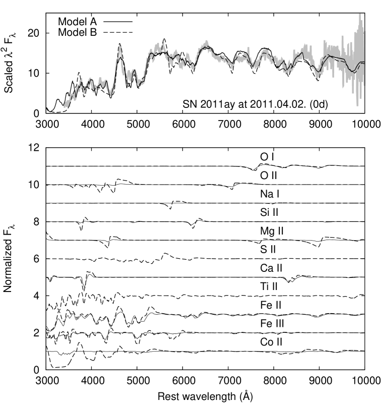
Figure 6: Single-ion contributions to the 0d spectrum fit (solid line = Model A, dashed line = Model B).

Table 5: The photospheric velocities and temperatures for Model A and B, as found by SYNAPPS

Date	Epoch	$v_{phot}^{A}$	$T_{phot}^{A}$	$v_{phot}^{B}$	$T_{phot}^{B}$
	(days)	(km s-1)	(K)	(km s-1)	(K)
March 24	$-9$	9830	8710	6500	10,000
March 31	$-2$	9640	7460	6500	10,000
April 02	0	9280	7260	6000	8760
April 05	+3	9090	6000	6500	8620
April 19	+17	8870	5300	4100	6490

The final best-fit model spectra for both Model A and Model B are plotted together with the observations in Fig. 5. Fig. 6 shows the single-ion contributions to the best-fit models for the +0d spectrum, i.e. at the phase of V-band maximum. The basic global parameters for both models are collected in Table 5.

From Table 5 and Figs 5 - 6 it is immediately apparent that, despite having quite different $v_{phot}$ values, both Model A and B give acceptable fits to the observed spectra. Both models reproduce the major spectral features well, although neither fits perfectly all the weak, narrow humps that become stronger in the post-maximum spectra. This is somewhat surprising, because the two models converged to $v_{phot}$ values that are different by $\sim 3000$ km s^-1. Since the uncertainty of the photospheric velocities derived by SYNAPPS are thought to be $\sim 500$ - $1000$ km s^-1, at least for SNe Ia (Parrent, 2014), such a high level of ambiguity, at first, seems to be unexpected. It is, however, not unprecedented among other SNe Iax: for example, Stritzinger et al. (2014) found similar inconsistency between their SYNAPPS models for the simulteneous optical ($v_{phot}\sim 4200$ km s^-1) and near-IR ($v_{phot}\sim 1700$ km s^-1) spectra of SN 2010ae at +18d phase.

A possible (and likely) explanation for this issue is that all modeled SN 2011ay spectra consist of heavily blended features, even at very early phases. There are no individual, unblended, single-ion features visible that can be identified unambiguously, except maybe O I $\lambda 7775$ in the pre-maximum spectra and the Ca II near-IR triplet after maximum. In both models considered here the presence of iron (both Fe II and Fe III) can be found at $-9$d, and blending with Fe II and Co II becomes excessively dominant at later phases, after maximum light. As noted by Branch et al. (2004), the “iron curtain” of strong Fe II prevented the secure identification of many other features in the post-maximum spectra of SN 2002cx, and this is exactly what we found here for SN 2011ay. The projected Doppler-velocities of blended features become quickly ill-constrained with the increasing number of overlapping lines from different ions.

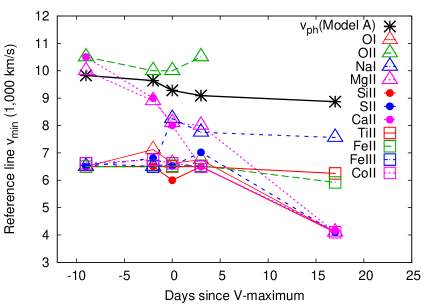
Figure 7: Evolution of the minimum velocities of the line-forming regions for each species in Model B. The uncertainty of these velocities is at least $\sim 1,000$ km s^-1. The lowest velocity at each phase corresponds to the photospheric velocity at the given epoch. For comparison, the photospheric velocity in Model A is also plotted with asterisks.

The evolution of the minimum velocities of the line forming region for each species in Model B are plotted in Fig. 7. On the contrary, Model A assumed that all features are formed with a minimum velocity of $v_{phot}$ as given in Table 5. It is apparent that while in Model B the photospheric velocity is significantly lower than that in Model A, Model B contains some low-mass ions (O II, Na I, Mg II) that are formed at higher velocities. The minimum velocities of these “detached” features are close to $v_{phot}$ of Model A, but they tend to decrease below that, and converge toward the photosphere at later phases (except for O II, which stays constantly at high velocity). Branch et al. (2004) also found similar “high-velocity” features in the spectra of SN 2002cx, but only at post-maximum phases. Fig. 7 suggests that such detached features forming at higher velocities may have appeared in SN 2011ay as early as 9-10 days before maximum.

From Fig. 5 and 6 it is seen that low-Z elements, such as O I, Na I, Mg II, start appearing at very early phases (more than one week pre-maximum), and they remain detectable even at post-maximum. S II may also be present (at least in Model B), which is often cited as a sign of thermonuclear explosion. These features are frequently observed in SNe Ia, but they are absent in SNe Ib/c.

Foley et al. (2013) reported the possible presence of carbon in SN 2011ay via the detection of C II $\lambda 6580$ and $\lambda 7234$ features, even though these features appear very weak (see Fig. 23 in Foley et al., 2013). We have checked the presence/absence of C I, C II or C III using SYNAPPS. The $-9$d and $-2$d spectra were selected for this purpose, because carbon features are expected to be the strongest during the pre-maximum phases. For this test we adopted Model B, because that model has similar velocities to those adopted by Foley et al. (2013).

As a first step, we simply added either C I, C II or C III to the best-fit Model B spectra to get carbon-enhanced models. The purpose of this step was to check which carbon features should be visible under the physical conditions corresponding to Model B. Fig. 8 shows these carbon-enhanced models together with the carbon-free models and the $-2$d and $-9$d observed spectra. Note that the carbon features are artificially enhanced for making their identification easier.

It is seen that large amount of C I or C III would cause observable features only at wavelengths longer than $8000$ Å  where the observed spectra have the lowest signal-to-noise and contamination from telluric lines is the strongest. Thus, the reliable identification of these ions is not possible from these spectra.

However, the C II $\lambda 6580$ and $\lambda 7234$ features offer better opportunity to detect carbon in the optical spectra. There is a feature in both the $-9$d and the $-2$d observed spectra that could be C II $\lambda 7234$, as found by Foley et al. (2013). Note that this feature is originally modeled with high-velocity O II in both Model A and B, which is not a secure identification (see below). Even though the simultaneous presence of the C II $\lambda 6580$ feature is not observed in the $-2$d spectrum, there may be a weak feature at the expected position in the $-9$d spectrum.

In order to test whether it is more appropriate to explain the feature around $7100$ Å with C II rather than O II, we replaced O II with C II in the best-fit $-9$d Model B spectrum, and recomputed the fitting. The excitation temperature for carbon was set variable to take into account the possibility for non-LTE excitations. It was found that $T_{exc}=20,000$ K (which is a factor of 2 higher than $T_{phot}$ at this phase) would indeed reduce the strength of the $\lambda 6580$ feature relative to that of the $\lambda 7234$ one.

In Fig. 9 the new carbon-enhanced model is compared with the original best-fit Model B spectrum (without carbon) and the observations. It is seen that while the C II $\lambda 7234$ feature is a similarly good fit to the observed spectrum as the high-velocity O II feature in the original model, this is not true for the C II $\lambda 6580$ feature, the latter being much stronger than the observed notch around $6400$ Å. Note that setting the excitation temperature of C II close to the photospheric temperature, $T_{phot}=10,000$ K, would make the $\lambda 6580$ feature even stronger, enhancing the inconsistency between the carbon-enhanced model and the observations. Thus, if C II were responsible for the observed feature at $\sim 7100$ Å  then the $\lambda 6580$ feature should appear much stronger than observed.

It is concluded that our SYNAPPS modeling does not confirm the detection of C II features in the pre-maximum optical spectra of SN 2011ay, and the same is true for both C I and C III.

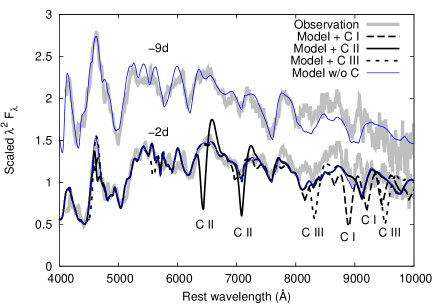
Figure 8: Modified Model B spectra containing artificially enhanced carbon features (thick solid and dashed lines) together with the $-2$d observed spectrum (grey curve) and the original, best-fit Model B spectrum without carbon (thin solid line). The observed and carbon-free model spectra at $-9$d are also shown for comparison.

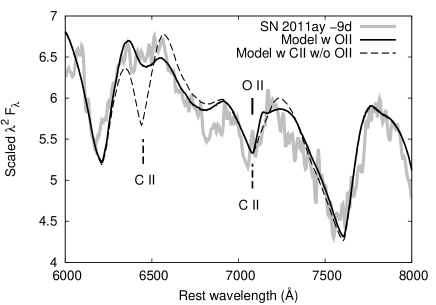
Figure 9: Comparison of the modified Model B containing C II instead of high-velocity OII (dashed line) with the original Model B (having OII, without CII, thick solid line) and the observed $-9$d spectrum (grey curve). If CII $\lambda 7234$ were present, $\lambda 6580$ would appear much stronger than observed (see text for details).

The identification of the $\lambda 7100$ feature as high-velocity O II in the early-phase spectra (see Fig. 6 and 7) is also uncertain. O II is usually absent in the pre-maximum spectra of SNe Ia, but it was found in other SNe Iax around maximum light, namely in 2008A and 2005hk, by McCully et al. (2014a). Given that our models for SN 2011ay have photospheric temperatures not exceeding 10,000 K (cf. Table 5), the appearance of O II with nearly the same strength as O I is not expected, at least in quasi-LTE conditions. Hatano et al. (1999) predicted equal optical depth for these two ions at $T\sim 12,000$ K, but note that they used $n_{e}\sim 5\times 10^{9}$ cm^-1 for the electron density, a typical value for SNe Ia-s. If the electron density in SN 2011ay were lower than this, then ionization would be more effective at a given temperature, thus, the O II features could become stronger even at $T<10,000$ K. Nevertheless, since it is based on only a single feature, the presence of O II in SN 2011ay cannot be proven unambiguously.

Regarding the intermediate-mass elements (IME), Ca II is close to the detection limit in the pre-maximum spectra, but its near-IR triplet (IR3) $\lambda 8579$ feature becomes very strong by two weeks after maximum. Similar behavior is observed in overluminuous SNe Ia-91T (see e.g. Phillips et al., 1992; Garavini et al., 2004), but those objects are characterized by very different light curve properties.

This kind of spectral evolution is the opposite of what is observed in normal SNe Ia (see e.g. Marion et al., 2013): in most SNe Ia the Ca II IR3 starts as a strong high-velocity feature (HVF) at $v\ {\raise-2.15277pt\hbox{$\buildrel>\over{\sim}$}}\ 20,000$ km s^-1 at about two weeks before maximum, while low-Z elements are absent or very weak. By the time of maximum light the Ca II HVF disappears, while its photospheric component (PVF, $v\sim 10,000$ km s^-1) gets stronger. O I $\lambda 7775$ can, sometimes, be detected as a HVF at very early phases (Parrent et al., 2012), but it is frequently absent and its PVF shows up only after maximum light.

It is seen in the spectra presented in this paper that SN 2011ay does not exhibit such kind of HVF for any ion at any phase observed. This also appears true for all other SNe Iax observed so far (Foley et al., 2013). It is interesting that the absence of Ca II HVF is also characteristic for the low-velocity, 91bg subtype of SNe Ia (Childress et al., 2014; Silverman et al., 2015).

Unlike the Ca II features, the Fe II lines appear quite strong in SN 2011ay, even during pre-maximum. The strong presence of Fe II at such early phases were not observed in most “normal” SNe Ia spectra. Also, they were not identified in other pre-maximum Iax spectra, e.g. SN 2002cx (Branch et al., 2004) or SN 2005hk (Sahu et al., 2008). Their strong appearance in SN 2011ay might be due to its cooler photospheric temperature during pre-maximum: $T_{phot}\leq 10,000$ K (Table 5). SNe Ia typically have $T_{phot}\ {\raise-2.15277pt\hbox{$\buildrel>\over{\sim}$}}\ 10,000$ K before maximum. Concerning other SNe Iax, Fe II features were found strong in the post-maximum spectra of SNe 2002cx (Branch et al., 2004) and 2005hk (Sahu et al., 2008), when the photospheric temperature cooled below $\sim 10,000$ K. After maximum light, Fe II and Ca II features dominate the observed spectra of SN 2011ay (Fig. 5), similar to SNe Ia.

3.3 Measuring velocities in SNe Iax spectra

One of the most intriguing properties of SNe Iax is their low expansion velocities (e.g. Branch et al., 2004; Foley et al., 2013), which can, in extreme cases, be as low as $\sim 2000$ km s^-1 (Stritzinger et al., 2014). This has been confirmed for multiple SNe Iax by spectral modeling with SYNOW/SYNAPPS, i.e. similar methodology to that which has been applied in this paper. To estimate the expansion velocity for a bigger sample of SNe Iax, Foley et al. (2013) used the projected Doppler-shift of the absorption minimum of the feature around $\lambda$6200 Å, which was interpreted as due to Si II $\lambda$6355, similar to Type Ia SNe. Based on this assumption, Foley et al. (2013) concluded that the “ejecta velocity”, $|v|$, defined this way is less than $8000$ km s^-1 for all SNe Iax. All SNe Iax spectra studied to date indeed show signs for significantly lower expansion velocities than most SNe Ia which usually have $v_{\mathrm{SiII}}>10,000$ km s^-1 around maximum light (e.g. Blondin et al., 2006), however, we show below that such “quick-look” velocity estimates based on single spectral features may lead to significantly under- or overestimated velocities for SNe Iax, which have much more complex spectra than SNe Ia.

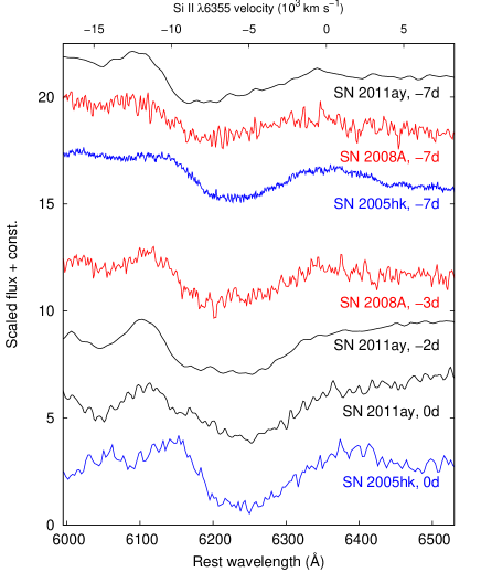
Figure 10: Comparison of the near-maximum spectra of three different SNe Iax in the region of 6000–6500 Å: SN 2005hk (Phillips et al., 2007), SN 2008A (Blondin et al., 2012), and SN 2011ay (present work and Foley et al., 2013). All epochs are given relative to V maxima. The spectra of SNe 2005hk and 2008A were downloaded from WISeREP (Yaron & Gal-Yam, 2012). A velocity scale relative to Si II $\lambda$6355 is also shown on the upper horizontal axis.

We focus on the feature appearing around $\sim\lambda$6200 Å in the pre-maximum spectra of SN 2011ay. Fig. 10 shows this feature before and around maximum light compared to two other SNe Iax observed at similar phases. It is seen that this feature is broad and shallow. In this respect, SN 2011ay and some other SNe Iax look similar to SNe Ia-91T (Branch et al., 2004; Foley et al., 2013), i.e. they usually show weaker Si II $\lambda$6355 lines compared to normal Ia-s. However, the post-maximum spectral evolution of the two classes of SNe are markedly different.

The first issue with the velocity measurement from this feature is related to its line strength. Jeffery & Branch (1990) studied the effects of line strength, ejecta density and other parameters on the Doppler-shift of the absorption minimum of P Cygni features in SN atmospheres. They showed that for features having optical depth $\tau\sim 1$ at the photosphere, the absorption minimum forms very close to $v_{phot}$. That is why the velocity from the Si II $\lambda$6355 feature gives so reasonable photospheric velocities in SNe Ia: this feature is strong and relatively unblended in SNe Ia (e.g. Parrent et al., 2012). For weak features having $\tau<1$, however, resonant scattering tends to dominate over absorption, which may shift the absorption minimum significantly below $v_{phot}$. On the contrary, much stronger features, like Ca II, tend to show absorption minima at velocities much higher than $v_{phot}$, as expected.

Fig. 10 suggests that SN 2011ay had similar photospheric velocity to SN 2008A, and both of them expanded faster than SN 2005hk. Using SYNAPPS, McCully et al. (2014a) derived $\sim 7000$ and $\sim 8500$ km s^-1 for 2005hk and 2008A, respectively, while Foley et al. (2013) estimated $\sim 4500$ and $\sim 6400$ km s^-1 from the $\lambda$6200 feature. The $\sim 2000$ km s^-1 difference between the single-feature and the spectrum-modeling velocity illustrates the issue of the velocity measurement in SNe Iax spectra. For SN 2011ay we find a similar conflict: at maximum light the single-feature velocity estimate gives $\sim 5600$ km s^-1 (Silverman et al., 2011; Foley et al., 2013), while our Model A predicts $v_{phot}\sim 9000$ km s^-1 (with an uncertainty of at least $\sim 1000$ km s^-1). It seems that SYNAPPS modeling tend to produce higher velocities than the single-feature “quick-look” estimates.

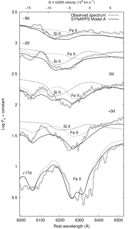
Figure 11: Spectral evolution of SN 2011ay between 6000–6500 Å. The observed spectrum (thick gray line) is plotted together with the SYNAPPS model from Model A (solid line) as well as single-ion contributions from Si II (dashed line) and Fe II (dotted line). Fe II $\lambda$6456 starts blending with Si II $\lambda$6355 a few days before maximum, and it becomes the dominant feature post-maximum. A velocity scale relative to Si II $\lambda$6355 is also shown on the upper horizontal axis.

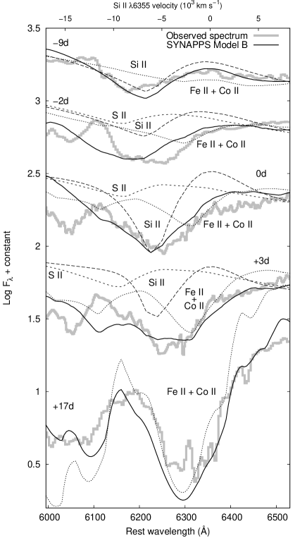
Figure 12: The same as Fig. 11 but showing Model B, and adding the single-ion contributions from S II and Co II. Complex blending between these features results in nearly the same observed spectra, even though the photospheric velocities are $\sim 3000$ km s^-1 less than in Model A.

However, there is an even bigger issue with the velocity measurement in SNe Iax spectra. This is the severe blending across the whole optical regime, which prevents any unique, secure line identification, as was detailed in the previous section. This affects the $\lambda$6200 feature, further plaguing the velocity determination.

Fig. 11 again zooms in the 6000 - 6500 Å regime while showing the observed spectral evolution of SN 2011ay together with the model spectra by Model A (i.e. the one having higher $v_{phot}$). From the single-ion contributions it is seen that the broad $\lambda$6200 feature is due to blending between Si II $\lambda$6355 and Fe  II $\lambda$6456, even during the pre-maximum phases. Similar blending is also visible in other SNe Iax, as found in 2002cx at +7d ($T_{BB}\sim 9000$ K, Li et al., 2003; Branch et al., 2004), 2005hk at -1d ($T_{BB}\sim 9000$ K, Phillips et al., 2007; Sahu et al., 2008), 2008A at -3d (McCully et al., 2014a), and 2010ae at +16d (Stritzinger et al., 2014). This blending broadens the observed profile and shifts the middle of the feature toward lower velocities, which may likely explain the discrepancies between the “quick-look” and the modeled velocities mentioned above.

Moreover, this is not yet the full story, because, as illustrated in Fig. 12, blending between the different single-ion features in this regime may result in nearly the same observed spectrum, even when the photospheric velocity is close to $\sim 6000$ km s^-1, i.e. close to what the “quick-look” velocity estimate predicts. Thus, even when using a sophisticated parametrized spectrum modeling code and putting in all possible features that likely contribute to the observed spectrum, the resulting model may still be ambiguous: if the observed spectrum consists of broad features and almost all of them are complex blends, then the photospheric velocity becomes rather ill-constrained.

A good example for this ambiguity is SN 2011ay: as shown in the previous section, its observed spectra can be explained either with $v_{phot}\sim 6000$ or $\sim 9000$ km s^-1 almost equally well. This and the appearance of the detached features (those having higher velocities than $v_{phot}$) in the lower velocity Model B might also be a hint for a multiple velocity structure in the ejecta, i.e. a disk-like or a jet-like configuration. Investigations of such models are beyond the scope of this paper, and might be possible only by having more extensive data coverage, both in wavelength (i.e. by adding infrared and/or UV spectra) and in time.

3.4 Spectral energy distributions and light-curve modeling

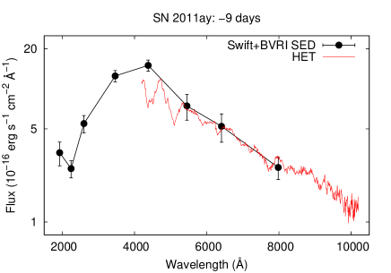
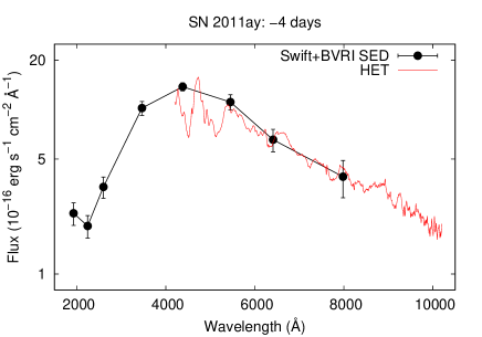
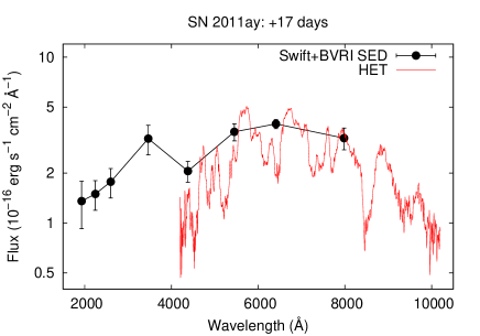
Figure 13: Scaled HET spectra and the UV-optical SEDs of SN 2011ay at different epochs relative to V maximum: -9 days (2011 March 24, top left), -4 days (2011 March 29, bottom left), +17 days (2011 April 19, bottom right).

To calculate the SEDs of SN 2011ay, we converted the BVRI and Swift/UVOT magnitudes to $F_{\lambda}$ fluxes using the calibration of Bessell, Castelli & Plez (1998). The fluxes were dereddened using the galactic reddening law parametrized by Fitzpatrick & Massa (2007) assuming $R_{V}=3.1$ and adopting $E(B-V)=0.081$ mag (§3.1.). The combined UV-optical SEDs are compared with the three HET spectra in Figure 13. After correcting for the small uncertainties in the absolute flux calibration of HET data, the spectra and the broadband SEDs match very well. Trustworthiness of Swift data at +17 days are lower, because SN 2011ay was already quite faint in the UV at that time.

The quasi-bolometric light curve was derived by integrating the dereddened $F_{\lambda}$ values of the combined UV-optical SEDs against wavelength. The long-wavelength contribution (not covered by these data) was estimated by fitting a Rayleigh-Jeans tail to the red end of the observed SEDs, and integrating it to infinity. In addition, the light curve was supplemented by two published KAIT-measurements: a non-detection on March 1 (2 455 621.7 JD), and the unfiltered magnitude at the discovery (Blanchard et al., 2011). The luminosity calculated from the latter was used as a lower limit at that epoch. Finally, the integrated fluxes were converted to luminosities using $D=86.9$ Mpc (see §1).

We applied a generalized analytic light curve model published by Chatzopoulos, Wheeler & Vinkó (2009, 2012) to derive the main parameters of the SN. This model is based on the radioactive decay diffusion model of Arnett (1982) and its generalized form by Valenti et al. (2008), but also takes into account the gamma-ray leakage from the ejecta. In this model the output luminosity can be expressed as

$$L(t)=M_{\mathrm{Ni}}\mathrm{e}^{-x^{2}}\left[\left(\epsilon_{\mathrm{Ni}}-\epsilon_{\mathrm{Co}}\right)\int_{0}^{x}2z\mathrm{e}^{z^{2}-2zy}\,\mathrm{d}z+\epsilon_{\mathrm{Co}}\right.$$

$$\left.\times\int_{0}^{x}2z\mathrm{e}^{z^{2}-2yz+2zs}\,\mathrm{d}z\right]\left(1-\mathrm{e}^{-At^{-2}}\right),$$ (3)

where $x=t/t_{\mathrm{m}}$, $t_{\mathrm{m}}$ is the effective diffusion time (roughly equal to the rise time to maximum), $y=t_{\mathrm{m}}/(2t_{\mathrm{Ni}})$ with $t_{\mathrm{Ni}}=8.8$ days, $s=t_{\mathrm{m}}(t_{\mathrm{Co}}-t_{\mathrm{Ni}})/(2t_{\mathrm{Co}}t_{\mathrm{Ni}})$ with $t_{\mathrm{Co}}=111.3$ days, $M_{\mathrm{Ni}}$ is the initial nickel mass, $\epsilon_{\mathrm{Ni}}=3.9\times 10^{10}$ erg s^-1 g^-1 and $\epsilon_{\mathrm{Co}}=6.8\times 10^{9}$ erg s^-1 g^-1 are the energy generation rates due to Ni- and Co-decay.

The last term of Eq. (3) describes the amount of gamma-ray leaking. Assuming a spherical uniform density ejecta with radius $R=vt$, homologous expansion (due to $t^{-2}$ scaling), and the Ni/Co confined in the center, yields $A=\left(3\kappa_{\gamma}M_{\mathrm{ej}}\right)/\left(4\pi v^{2}\right)$, where $\kappa_{\gamma}$ is the gamma-ray opacity, $M_{\mathrm{ej}}$ is the ejecta mass. Note that we used the dimensionless form of $\left(1-\exp\left(-A_{\mathrm{norm}}\cdot t_{10}^{-2}\right)\right)$, where $t_{10}\equiv$ $t$/10 days.

The quasi-bolometric light curve and the best-fitting model are shown in Figure 14. The corresponding parameters are presented in Table 6. Both the nickel mass ($\sim 0.22$ $M_{\odot}$) and the rise time ($\sim 14$ d) are lower than the usual values for SNe Ia ($\sim 0.6$ $M_{\odot}$ and $\sim 18$ d, respectively) , similar to the conclusion by Foley et al. (2013). The short rise time implies low ejecta mass. Following the method applied by Foley et al. (2009) for SN 2008ha and assuming that the ejecta of SN 2011ay has the same mean opacity as that of a normal SN Ia, we have

$$E_{\mathrm{kin}}/E_{\mathrm{kin,Ia}}=\left(\frac{v}{v_{\mathrm{Ia}}}\right)^{3}\left(\frac{t_{\mathrm{rise}}}{t_{\mathrm{rise,Ia}}}\right)^{2}$$ (4)

and

$$M_{\mathrm{ej}}/M_{\mathrm{ej,Ia}}=\frac{v}{v_{\mathrm{Ia}}}\left(\frac{t_{\mathrm{rise}}}{t_{\mathrm{rise,Ia}}}\right)^{2}.$$ (5)

Adopting $v\sim 9,300$ km s^-1, as suggested by the higher-velocity Model A (§3.2) and $t_{\mathrm{rise}}$ = 14 days together with the reference values of $E_{\mathrm{kin,Ia}}$ = 10⁵¹ erg, $M_{\mathrm{ej,Ia}}$ = 1.4 $M_{\odot}$, $v_{\mathrm{Ia}}$ = 10 000 km s^-1 (Foley et al., 2009) and the average value of $t_{\mathrm{rise,Ia}}$ = 18.0 days (see Ganeshalingam, Li & Filippenko, 2011), these formulae result in $E_{\mathrm{kin}}$ = 0.5$\cdot$10⁵¹ erg and $M_{\mathrm{ej}}$ = 0.8 $M_{\odot}$ as the kinetic energy and the ejecta mass of SN 2011ay, respectively. Alternatively, using $v\sim 6000$ km s^-1 from the lower-velocity Model B results in $M_{\mathrm{ej}}\sim 0.5M_{\odot}$ and $E_{\mathrm{kin}}=0.1\cdot$10⁵¹ erg. The ejecta mass and expansion energy estimated this way are consistent with previous findings for SNe Iax. The lower nickel mass, $M_{\mathrm{Ni}}\sim 0.2$ $M_{\odot}$ as calculated from the Arnett-model, also suggests that the explosion, if indeed thermonuclear, may be less energetic that in Type Ia-s.

Table 6: Physical parameters determined from the modeling of the bolometric light curve.

$t_{0}$ (JD)	2 455 633.0 $\pm$ 1.5	Date of explosion
$t_{\mathrm{rise}}$ (d)	14 $\pm$ 1	Rise time to maximum
$M_{\mathrm{Ni}}$ ($M_{\odot}$)	0.225 $\pm$ 0.010	Initial 56Ni mass
$A_{\mathrm{norm}}^{a}$	25 $\pm$ 7	$\gamma$-ray leakage parameter

Notes. ^aThe parameter connected to gamma-ray leaking (see Eq. 3 and text for details).

Figure 14: Quasi-bolometric light curve of SN 2011ay with the best-fitting Arnett-model (solid line) and the one with assuming full gamma-ray trapping (dashed line). The first two luminosities were calculated from the measurements of Blanchard et al. (2011), see the text for details.

4 Discussion and conclusions

Based on photometric and spectroscopic data obtained during the early phases we carried out a detailed analysis on SN 2011ay, one of the members of the recently defined class of SNe Iax. The spectra as well as the light and color curves are similar to those of other objects belonging to this group (see Foley et al., 2013, and references therein).

We calculated model spectra with the parametrized modeling code SYNAPPS to get more information on the spectral evolution and the physical properties of the ejecta. As presented in Section 3.2, the spectral characteristics of SN 2011ay are basically similar to those of other SNe Iax. We found that Fe II features appear even before maximum, which can be explained with the relatively lower photospheric temperature ($T_{phot}\sim$ 8,000 K) of the ejecta.

The presence of Fe II and other features that cause severe blending across the entire visible spectral domain makes the direct analysis of such spectra very difficult and ambiguous. We found that it is possible to fit most of the broad features of SN 2011ay by two models (Model A and B) that have similar chemical composition but very different photospheric velocity ($\sim 9,300$ km s^-1 and $\sim 6,000$ km s^-1 at maximum, respectively).

The effect of strong blending also makes the “quick-look” velocity estimates uncertain. We showed in Section 3.3 that measuring the absorption minimum of the $\lambda$6200 feature and assuming that it is due to purely Si II $\lambda$6355 might underestimate $v_{phot}$, because of the effect of blending with Fe II and Co II. This does not question the fact that SNe Iax generally have lower expansion velocities than SNe Ia, but the non-uniqueness of the spectrum modeling fits presented in this paper makes the velocities of such events rather ill-constrained.

Fitting a radiative-diffusion model (taking into account gamma-ray leaking) to the quasi-bolometric light curve of SN 2011ay resulted in physical parameters for the rise time to maximum, ejecta mass, initial nickel mass and kinetic energy that are all below their mean value for SNe Ia, as pointed out by Foley et al. (2013). Although SN 2011ay seems to be close to the upper limits of these parameters, it clearly belongs to the recently defined class: the values of ⁵⁶Ni mass and total ejecta mass (0.225$\pm$0.010 $M_{\odot}$ and $\sim$0.8 $M_{\odot}$, respectively) are similar to the parameters of other, bright (M${}_{V}>$ -18 mag) SNe Iax (SNe 2005hk, 2008A, 2009ku; see Foley et al., 2013; McCully et al., 2014a). Note that in addition to the criteria defined by Foley et al. (2013), the faster decline rate of the bolometric light curve, indicated by the relatively low value of the gamma-ray trapping parameter $A_{norm}$ (see Table 6), may also be characteristic for SNe Iax.

The results of the light curve modeling strengthen the picture that the progenitor of SN 2011ay is likely an incompletely exploded white dwarf, which seems to be the best explanation of this kind of SNe to date. The presence of Si II and S II features in the early spectra of SN 2011ay in Figure 5 may be signs of thermonuclear explosion, which might give additional support for the white dwarf explosion scenario.

These results, as well as other detailed studies of single events, may help us to understand better the properties of type Iax SNe. However, there are still a lot of open questions about the true nature and origin of this class of stellar explosions.

References

- Arnett (1982) Arnett W. D., 1982, ApJ, 253, 785
- Bessell, Castelli & Plez (1998) Bessell M. S., Castelli F., Plez B., 1998, A&A, 333, 231
- Bildsten (2007) Bildsten L., Shen K.J., Weinberg N.N., Nelemans G., 2007, ApJ, 662, L95
- Blanchard et al. (2011) Blanchard P. et al., 2011, CBET 2678
- Blondin et al. (2006) Blondin S. et al., 2006, AJ, 131, 1648
- Blondin et al. (2012) Blondin S. et al., 2012, AJ, 143, 126
- Blondin & Tonry (2007) Blondin S., Tonry J.L., 2007, ApJ, 666, 1024
- Branch et al. (2004) Branch D., Baron E., Thomas R. C., Kasen D., Li W., Filippenko A. V., 2004, PASP, 116, 903
- Chatzopoulos, Wheeler & Vinkó (2009) Chatzopoulos E., Wheeler J. C., Vinkó J., 2009, ApJ, 704, 1251
- Chatzopoulos, Wheeler & Vinkó (2012) Chatzopoulos E., Wheeler J. C., Vinkó J., 2012, ApJ, 746, 121
- Childress et al. (2014) Childress M. J., Filippenko A. V., Ganeshalingam M., Schmidt B. P., 2014, MNRAS, 437, 338
- Chornock et al. (2006) Chornock R., Filippenko A. V., Branch D., Foley R. J., Jha S., Li W., 2006, PASP, 118, 722
- Fitzpatrick & Massa (2007) Fitzpatrick E. L., Massa D., 2007, ApJ, 663, 320
- Foley et al. (2009) Foley R. J. et al., 2009, AJ, 138, 376
- Foley et al. (2010a) Foley R. J., Brown P.J., Rest A., Challis P.J., Kirshner R.P., Wood-Vasey W.M., 2010a, ApJ, 708, 1748
- Foley et al. (2010b) Foley R. J. et al., 2010b, AJ, 140, 1321
- Foley et al. (2013) Foley R. J. et al., 2013, ApJ, 767, 57
- Foley et al. (2015) Foley R. J., Van Dyk S. D., Jha S. W., Clubb K. I., Filippenko A. V., Mauerhan J. C., Miller A. A., Smith N., 2015, ApJ, 798, L37
- Ganeshalingam, Li & Filippenko (2011) Ganeshalingam M., Li W., Filippenko A. V., 2011, MNRAS, 416, 2607
- Garavini et al. (2004) Garavini G. et al., 2004, AJ, 128, 387
- Hatano et al. (1999) Hatano K., Branch D., Fisher A., Millard J., Baron E., 1999, ApJS, 121, 233
- Hill et al. (1998) Hill G. J., MacQueen P. J., Nicklas H., Cobos D. F. J., Tejada C., Mitsch W., Wolf M. J., 1998, in D’Odorico S., ed., Society of Photo-Optical Instrumentation Engineers (SPIE) Conference Series Vol. 3355 of Society of Photo-Optical Instrumentation Engineers (SPIE) Conference Series, Hobby-Eberly Telescope low-resolution spectrograph: mechanical design. pp 433–443
- Jeffery & Branch (1990) Jeffery D. J., Branch D., 1990, sjws.conf, 149
- Jha et al. (2006) Jha S., Branch D., Chornock R., Foley R. J., Li W., Swift B. J., Casebeer D., Filippenko A. V., 2006, AJ, 132, 189
- Jordan et al. (2012) Jordan IV G. C., Perets H. B., Fisher R. T., van Rossum D. R., 2012, ApJ, 761, L23
- Jordi, Grebel & Ammon (2006) Jordi K., Grebel E. K., Ammon K., 2006, A&A, 460, 339
- Krömer et al. (2013) Krömer M. et al., 2013, MNRAS, 429, 2287
- Li et al. (2003) Li W. et al., 2003, PASP, 115, 453
- Lyman et al. (2013) Lyman J. D., James P. A., Perets H. B., Anderson J. P., Gal-Yam A., Mazzali P., Percival S. M., 2013, MNRAS, 434, 527
- Marion et al. (2013) Marion G. H. et al., 2013, ApJ, 777, 40
- McClelland et al. (2010) McClelland C. M. et al., 2010, ApJ, 720, 704
- McCully et al. (2014a) McCully C. et al., 2014a, ApJ, 786, 134
- McCully et al. (2014b) McCully C. et al., 2014b, Nature, 512, 54
- Miller & Owen (2001) Miller N. A., Owen F. N., 2001, ApJS, 134, 355
- Moriya et al. (2010) Moriya T., Tominaga N., Tanaka M., Nomoto K., Sauer D. N., Mazzali P. A., Maeda K., Suzuki T., 2010, ApJ, 719, 1445
- Narayan et al. (2011) Narayan G. et al., 2011, ApJ, 731, L11
- Parrent et al. (2012) Parrent J. T. et al., 2012, ApJ, 752, L26
- Parrent (2014) Parrent J. T., 2014, arXiv, arXiv:1412.7163
- Parrent, Friesen & Parthasarathy (2014) Parrent J. T., Friesen B., Parthasarathy M., 2014, Ap&SS, 351, 1
- Phillips et al. (1992) Phillips M. M., Wells L. A., Suntzeff N. B., Hamuy M., Leibundgut B., Kirschner R. P., Foltz C. B., 1992, AJ, 103, 1632
- Phillips et al. (2007) Phillips M. M. et al., 2007, PASP, 119, 360
- Pogge, Garnavich & Pedani (2011) Pogge R. W., Garnavich P. M., Pedani M., 2011, CBET, 2678
- Sahu et al. (2008) Sahu D. K. et al., 2008, ApJ, 680, 580
- Schlafly & Finkbeiner (2011) Schlafly E. F., Finkbeiner D. P., 2011, ApJ, 737, 13
- Silverman et al. (2011) Silverman J. M., Filippenko A. V., Barth A. J., Walsh J. L., Assef R. J., 2011, CBET, 2681
- Silverman et al. (2015) Silverman J. M., Vinkó J., Marion G. H., Wheeler J. C., Barna B., Szalai T., Mulligan B. W., Filippenko A. V., 2015, arXiv, arXiv:1502.07278
- Stritzinger et al. (2014) Stritzinger M. D. et al., 2014, A&A, 561, 146
- Stritzinger et al. (2015) Stritzinger M. D. et al., 2015, A&A, 573, 2
- Takáts & Vinkó (2012) Takáts K., Vinkó J., 2012, MNRAS, 419, 2783
- Thomas, Nugent & Meza (2011) Thomas R. C., Nugent P. E., Meza J. C., 2011, PASP, 123, 237
- Valenti et al. (2008) Valenti S. et al., 2008, MNRAS, 383, 1485
- Valenti et al. (2009) Valenti S. et al., 2009, Nature, 459, 674
- Wang, Justham & Han (2013) Wang B., Justham S., Han Z., 2013, A&A, 559, 94
- Yamanaka et al. (2015) Yamanaka M. et al., 2015, arXiv, arXiv:1505.01593
- Yaron & Gal-Yam (2012) Yaron O., Gal-Yam A., 2012, PASP, 124, 668