Stable oscillation in spin torque oscillator excited by a small in-plane magnetic field

Abstract

Theoretical conditions to excite self-oscillation in a spin torque oscillator consisting of a perpendicularly magnetized free layer and an in-plane magnetized pinned layer are investigated by analytically solving the Landau-Lifshitz-Gilbert equation. The analytical relation between the current and oscillation frequency is derived. It is found that a large amplitude oscillation can be excited by applying a small field pointing to the direction anti-parallel to the magnetization of the pinned layer. The validity of the analytical results is confirmed by comparing with numerical simulation, showing good agreement especially in a low current region.

I Introduction

High-frequency devices are in demand for practical applications such as communication devices, magnetic sensors, and measurement systems. Spin torque oscillator (STO) Slonczewski (1996); Berger (1996); Kiselev et al. (2003); Rippard et al. (2004); Houssameddine et al. (2007); Pribiag et al. (2007); Mistral et al. (2008); Kudo et al. (2009); Dussaux et al. (2010); Zeng et al. (2012); Kubota et al. (2013); Lebrun et al. (2014) is a promising candidate for such applications because high-frequency signal on the order of Gigahertz can be achieved through the giant magnetoresistance (GMR) or tunnel magnetoresistance (TMR) effect. A small size on the order of nano-meter, a wide frequency tunability over than one Gigahertz, and a narrow linewidth less than one Megahertz are also preferable features for device applications. In particular, an STO consisting of a perpendicularly magnetized free layer Yakata et al. (2009); Ikeda et al. (2010); Kubota et al. (2012) and an in-plane magnetized pinned layer has attracted much attention recently Kubota et al. (2013) because the large relative angle of the magnetizations of the free and pinned layers results in a large emission power on the order of 1 $\mu$W Kubota et al. (2013). Therefore, this type of STO is considered to be the model structure for practical applications.

The self-oscillation of the magnetization in an STO is excited when several conditions, such as the direction and magnitude of an applied field, are satisfied Bertotti et al. (2009); Ebels et al. (2008); Silva and Keller (2010); Gusakova et al. (2011); Khalsa et al. (2015); Taniguchi et al. (2013a); Taniguchi (2014); Pinna et al. (2014); Taniguchi (2015). While general conditions to excite the self-oscillation had been formulated Bertotti et al. (2009); Slavin and Tiberkevich (2009); Kim (2012), the possibility to excite the self-oscillation has to be investigated for each problems by solving the Landau-Lifshitz-Gilbert (LLG) equation. The number of theoretical works studying the conditions of the self-oscillation is few because of the complexity arising from the nonlinearity of the LLG equation. For example, the oscillation properties of STO with the perpendicularly magnetized free layer and the in-plane magnetized pinned layer were theoretically studied only in the presence of a perpendicular field Taniguchi et al. (2013a), in which the axial symmetry of the system reduces the difficulty to solve the LLG equation. On the other hand, it is still unclear whether the self-oscillation can be excited when the field direction is changed. It is practically important to investigate the possibility to excite self-oscillation in the presence of a field in a different direction due to the following reasons. For example in the sensor applications, an external magnetic field to be detected points to an arbitrary direction. Thus, it is insufficient to study the oscillation properties in the presence of a perpendicular field only. Another reason relates to the low power consumption. Our previous work Taniguchi et al. (2013a) showed that the zero-field oscillation is impossible in this type of STO, and a relatively high field is necessary to stabilize the self-oscillation by a perpendicular field. Discovering a method to excite a stable oscillation by a small field is therefore attractive from the viewpoint of reducing the power consumption of the STO. The change of the field direction might open a new possibility to this problem.

In this paper, we investigate the oscillation properties of the STO in the presence of an in-plane magnetic field by solving the LLG equation analytically. We find that an applied field smaller than Eq. (16) pointing in the direction anti-parallel to the magnetization of the pinned layer enables to excite a stable self-oscillation. This is a preferable feature for practical applications, compared with the oscillation by a perpendicular field in which relatively large field is required to stabilize the oscillation Taniguchi et al. (2013a). The relation between the current density and the oscillation frequency is derived. The comparison with numerical simulation guarantees the validity of the theory in the low current region.

The paper is organized as follows. In Sec. II, we derived the analytical formulas of the work done by spin torque and the dissipation due to damping, which are necessary to discuss the possibility to excite self-oscillation, by solving the LLG equation. Using these results, we discuss the theoretical conditions to excite the self-oscillation by an in-plane magnetic field in Sec. III These analytical discussions are compared with the numerical simulation in Sec. IV Section V is devoted to the discussion. Section VI provides our conclusion.

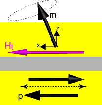
Figure 1: Schematic views of STO under consideration. An applied magnetic field points to the positive $x$-direction, whereas the magnetization of the pinned layer is parallel ($\mathbf{p}=+\mathbf{e}_{x}$) or anti-parallel ($\mathbf{p}=-\mathbf{e}_{x}$) to the applied field.

II Analytical Solution of LLG Equation

The system we consider is schematically shown in Fig. 1. The unit vectors pointing in the magnetization directions of the free and pinned layers are denoted as $\mathbf{m}$ and $\mathbf{p}$. We assume that the applied magnetic field points to the positive $x$-direction, whereas $\mathbf{p}$ is parallel or anti-parallel to the field. We use the macrospin model in this paper because its accuracy was confirmed by recent experiment Kubota et al. (2013). The LLG equation is given by

$$\frac{d\mathbf{m}}{dt}=-\gamma\mathbf{m}\times\mathbf{H}-\gamma H_{\rm s}\mathbf{m}\times\left(\mathbf{p}\times\mathbf{m}\right)+\alpha\mathbf{m}\times\frac{d\mathbf{m}}{dt},$$ (1)

where $\gamma$ and $\alpha$ are the gyromagnetic ratio and the Gilbert damping constant, respectively. In the following, we neglect higher order terms of $\alpha$ by assuming that $\alpha\ll 1$, which was confirmed experimentally Oogane et al. (2006); Konoto et al. (2013); Iihama et al. (2014). The magnetic field $\mathbf{H}$ consists of an effective perpendicular anisotropy $H_{\rm K}^{\rm eff}$ and the in-plane magnetic field $H_{\rm t}$ as

$$\mathbf{H}=H_{\rm t}\mathbf{e}_{x}+H_{\rm K}^{\rm eff}m_{z}\mathbf{e}_{z}.$$ (2)

The effective anisotropy is defined as $H_{\rm K}^{\rm eff}=H_{\rm K}-4\pi M$, where $H_{\rm K}$ is a crystalline anisotropy while $4\pi M$ is a shape anisotropy. The magnitude of the applied field is $H_{\rm t}(>0)$. The magnetic field is defined as a gradient of energy density $E$ as $\mathbf{H}=-\partial E/\partial(M\mathbf{m})$, where

$$E=-MH_{\rm t}m_{x}-\frac{MH_{\rm K}^{\rm eff}}{2}m_{z}^{2}.$$ (3)

A spin torque strength $H_{\rm s}$ is given by Slonczewski (1989, 2005)

$$H_{\rm s}=\frac{\hbar\eta j}{2e(1+\lambda\mathbf{m}\cdot\mathbf{p})Md},$$ (4)

where $d$ is the thickness of the free layer. The spin polarization of the pinned layer is $\eta$. The parameter $\lambda$ determines the dependence of the spin torque strength on the relative angle of the magnetizations, and is usually positive Slonczewski (1989, 2005); Xiao et al. (2004).

The self-oscillation can be excited when the energy supplied by the spin torque balances the dissipation due to damping, and thereby, the magnetization precesses on a constant energy curve of $E$. This condition can be expressed as $\mathscr{W}_{\rm s}+\mathscr{W}_{\alpha}=0$, where $\mathscr{W}_{\rm s}(E)=\gamma M\oint dtH_{\rm s}[\mathbf{p}\cdot\mathbf{H}-(\mathbf{m}\cdot\mathbf{p})(\mathbf{m}\cdot\mathbf{H})]$ and $\mathscr{W}_{\alpha}(E)=-\alpha\gamma M\oint dt[\mathbf{H}^{2}-(\mathbf{m}\cdot\mathbf{H})^{2}]$ are the work done by spin torque and the dissipation due to damping during a precession on the constant energy curve of $E$, respectively. This averaging technique over a constant energy curve was developed by several authors to investigate the magnetization switching rate in the thermally activated region and the oscillation properties in a ferromagnetic multilayer Bertotti et al. (2009, 2004, 2006); Serpico et al. (2005); Apalkov and Visscher (2005); Hillebrands and Thiaville (2006); Dykman (2012); Newhall and Eijnden (2013); Taniguchi et al. (2013b). In general, the magnetization dynamics in the macrospin model is described by two variables. The zenith and azimuth angles, or the three components in Cartesian coordinate with the constrain $|\mathbf{m}|=1$, are often used as the variables. Instead, energy $E$ and an angle $\psi$ can be chosen as the two variables, where $\psi$ characterizes the angle of the magnetization on a constant energy curve of $E$ Dykman (2012). The averaging technique over the constant energy curve integrates any quantity over $0\leq\psi\leq 2\pi$, and reduces the number of the variable to one, $E$. The reduction of the number of the variables makes it relatively easy to solve the LLG equation. However, there is still a technical difficulty to analytically investigate the possibility to excite self-oscillation arising from the calculations of $\mathscr{W}_{\rm s}$ and $\mathscr{W}_{\alpha}$. To calculate these functions, the solution of the precession trajectory of the magnetization on a constant energy curve, which is described by $d\mathbf{m}/dt=-\gamma\mathbf{m}\times\mathbf{H}$, should be derived. In the case of a perpendicular field previously studied Taniguchi et al. (2013a), such a trajectory is described by trigonometric functions, and the calculations of $\mathscr{W}_{\rm s}$ and $\mathscr{W}_{\alpha}$ become easy. On the other hand, in the case of an in-plane field, the precession trajectory on the constant energy curve is described by elliptic functions. In this case, several mathematical formulas are necessary to derive the explicit forms of $\mathscr{W}_{\rm s}$ and $\mathscr{W}_{\alpha}$. The details of the derivation of $\mathscr{W}_{\rm s}$ and $\mathscr{W}_{\alpha}$ in the present system are summarized in Appendix. Here, we show that the explicit forms of $\mathscr{W}_{\rm s}$ and $\mathscr{W}_{\alpha}$ are given by

$$\begin{split}\mathscr{W}_{\rm s}(E)&=\frac{\hbar\eta j}{ed}\sqrt{\frac{r_{1}-r_{3}}{H_{\rm K}^{\rm eff}/(2H_{\rm t})}}\mathcal{N}_{\rm s},\end{split}$$ (5)

$$\begin{split}\mathscr{W}_{\alpha}(E)&=-\frac{4\alpha M}{3}\sqrt{\frac{r_{1}-r_{3}}{H_{\rm K}^{\rm eff}/(2H_{\rm t})}}\mathcal{H}_{\alpha}.\end{split}$$ (6)

The functions $\mathcal{N}_{\rm s}$ and $\mathcal{H}_{\alpha}$ are given by

$$\begin{split}\mathcal{N}_{\rm s}=\mp&\left[\frac{(1\pm\lambda r_{1})}{\lambda^{2}(r_{1}-r_{3})}\mathsf{K}(k)\pm\frac{1}{\lambda}\mathsf{E}(k)\right.\\ &\left.-\frac{1+\lambda^{2}\pm 2\lambda r_{1}}{\lambda^{2}(r_{1}-r_{3})(1\pm\lambda r_{3})}\Pi(k,n)\right],\end{split}$$ (7)

$$\begin{split}\mathcal{H}_{\alpha}=&H_{\rm t}\left(\frac{1-r_{1}^{2}}{r_{1}-r_{3}}\right)\mathsf{K}(k)+\left(\frac{5E}{M}+3H_{\rm K}^{\rm eff}+\frac{2H_{\rm t}^{2}}{H_{\rm K}^{\rm eff}}\right)\mathsf{E}(k),\end{split}$$ (8)

where $r_{\ell}$ ($\ell=1,2,3$) are given by Eqs. (23), (24), and (25). The double sign in Eq. (7) means the upper when $\mathbf{p}$ is parallel to the applied field ($\mathbf{p}=+\mathbf{e}_{x}$) and the lower when $\mathbf{p}$ is anti-parallel to the applied field ($\mathbf{p}=-\mathbf{e}_{x}$). The first, second, and third kind of complete elliptic integrals are denoted as $\mathsf{K}(k)$, $\mathsf{E}(k)$ and $\Pi(k,n)$, respectively, where

$$k=\sqrt{\frac{r_{2}-r_{3}}{r_{1}-r_{3}}},$$ (9)

$$n=\frac{\mp\lambda(r_{2}-r_{3})}{1\pm\lambda r_{3}},$$ (10)

are the modulus and characteristic of the elliptic integral, respectively; see Appendix. Equation (5) is newly derived in this paper, while Eq. (6) was obtained in Ref. Taniguchi (2015).

Equations (5) and (6) are functions of the energy density. The range of the energy density is $E_{\rm min}<E<E_{\rm saddle}$, where $E_{\rm min}=-(MH_{\rm K}/2)[1+(H_{\rm t}/H_{\rm K})^{2}]$ and $E_{\rm saddle}=-MH_{\rm t}$ are the minimum and saddle point energies, respectively. The minimum energy point and the saddle point locate at $\mathbf{m}_{\rm min}=(H_{\rm t}/H_{\rm K}^{\rm eff},0,\sqrt{1-(H_{\rm t}/H_{\rm K}^{\rm eff})^{2}})$ and $\mathbf{m}_{\rm saddle}=(1,0,0)$. The precession period on the constant energy curve of $E$

$$\tau(E)=\frac{2\mathsf{K}(k)}{\gamma\sqrt{H_{\rm t}H_{\rm K}^{\rm eff}/2}\sqrt{r_{1}-r_{3}}},$$ (11)

relates to the oscillation frequency $f(E)$ via

$$f(E)=\frac{1}{\tau(E)}.$$ (12)

III Analytical Prediction on Possibility to Excite Self-Oscillation

Let us discuss the possibility to excite the self-oscillation in this system. We denote the current density satisfying $\mathscr{W}_{\rm s}(E)+\mathscr{W}_{\alpha}(E)=0$ as $j(E)$,

$$j(E)=\frac{4\alpha eMd}{3\hbar\eta}\frac{\mathcal{H}_{\alpha}}{\mathcal{N}_{\rm s}}.$$ (13)

The current $j(E)$ in the limit of $E\to E_{\rm min}$ is the critical current destabilizing the magnetization in equilibrium, which is obtained from the linearized LLG equation as

$$j_{\rm c}=\frac{2\alpha eMd}{\hbar\eta\mathcal{P}}H_{\rm K}^{\rm eff}\left[1-\frac{1}{2}\left(\frac{H_{\rm t}}{H_{\rm K}^{\rm eff}}\right)^{2}\right],$$ (14)

where $\mathcal{P}$ is

$$\mathcal{P}=\pm\left\{\frac{(H_{\rm t}/H_{\rm K}^{\rm eff})}{1\pm\lambda(H_{\rm t}/H_{\rm K}^{\rm eff})}\pm\frac{\lambda[1-(H_{\rm t}/H_{\rm K}^{\rm eff})^{2}]}{2[1\pm\lambda(H_{\rm t}/H_{\rm K}^{\rm eff})]^{2}}\right\}.$$ (15)

The double sign in Eq. (15) means the upper for $\mathbf{p}=+\mathbf{e}_{x}$ and lower for $\mathbf{p}=-\mathbf{e}_{x}$. We note here for the later discussion that $j_{\rm c}$ for $\mathbf{p}=-\mathbf{e}_{x}$ changes its sign when the applied field magnitude $H_{\rm t}$ becomes

$$\widetilde{H}_{\rm t}=\frac{(1-\sqrt{1-\lambda^{2}})}{\lambda}H_{\rm K}^{\rm eff},$$ (16)

whereas $j_{\rm c}$ for $\mathbf{p}=+\mathbf{e}_{x}$ does not. As discussed below, the oscillation properties of this type of STO is characterized solely by this critical current $I_{\rm c}$. This is particularly different from other type of STO consisting of an in-plane magnetized free layer, where two critical currents are necessary to distinguish the in-plane and out-of-plane oscillations Pinna et al. (2014); Newhall and Eijnden (2013); Hillebrands and Thiaville (2006); Taniguchi et al. (2013b). The number of such critical currents, as well as their values, is determined by the symmetry of the magnetic anisotropy and angular dependence of the spin torque, and should be investigated for each system.

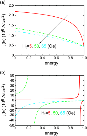
Figure 2: The dependence of $j(E)$ on $E$ for (a) $\mathbf{p}=+\mathbf{e}_{x}$ and (b) $\mathbf{p}=-\mathbf{e}_{x}$. The values of the applied field $H_{\rm t}$ are 5 (solid, red), 50 (dotted, green), and 65 (dashed, blue) Oe, respectively. The energy density in the horizontal axis $E$ is normalized as $(E-E_{\rm min})/(E_{\rm saddle}-E_{\rm min})$ to make $E_{\rm min}=0$ and $E_{\rm saddle}=1$.

Two conditions should be satisfied to excite self-oscillation on a constant energy curve of $E$ Taniguchi (2015). The first one is that $j(E)$ is finite. More practically, $j(E)$ should be experimentally available value, which is at maximum on the order of $10^{7}-10^{8}$ A/cm² in typical STOs Kiselev et al. (2003); Rippard et al. (2004); Houssameddine et al. (2007); Pribiag et al. (2007); Dussaux et al. (2010); Zeng et al. (2012); Kubota et al. (2013). The second is that $j(E)/j_{\rm c}>1$. This condition relates to the fact that a current larger than $j_{\rm c}$ should be applied to excite any kind of magnetization dynamics because the magnetization initially stays at the minimum energy state. If this condition is not satisfied, the magnetization moves to the constant energy curve including $E_{\rm saddle}$, and eventually stops its dynamics Taniguchi (2015). Let us study whether these conditions are satisfied for $\mathbf{p}=\pm\mathbf{e}_{x}$. The values of the parameters are taken from the experiments Kubota et al. (2013), where $M=1448$ emu/c.c., $H_{\rm K}=18.6$ kOe, $d=2$ nm, $\eta=0.54$, $\lambda=\eta^{2}$, $\gamma=1.732\times 10^{7}$ rad/(Oe$\cdot$s), and $\alpha=0.005$. The value of $\tilde{H}_{\rm t}$ is 61 Oe. The dependences of $j(E)$ on $E$ for $\mathbf{p}=+\mathbf{e}_{x}$ and $\mathbf{p}=-\mathbf{e}_{x}$ are shown in Figs. 2 (a) and (b), respectively. The values of $H_{\rm t}$ in Fig. 2 are chosen as $5$, $50$, and $65$ Oe to show $j(E)$ for both $H_{\rm t}<\widetilde{H}_{\rm t}$ and $H_{\rm t}>\widetilde{H}_{\rm t}$.

First, we discuss the possibility to excite self-oscillation when the magnetization of the pinned layer is parallel to the applied field ($\mathbf{p}=+\mathbf{e}_{x}$). The current $j(E)$ shown in Fig. 2 (a) indicates that $j(E)/j_{\rm c}<1$ for $E>E_{\rm min}$, meaning that the second condition mentioned above is not satisfied. Therefore, a stable oscillation cannot be excited when $\mathbf{p}$ is parallel to the applied field. This argument will be confirmed in Fig. 3 (a) below.

Next, we discuss the physical interpretation obtained from Fig. 2 (b), where the magnetization of the pinned layer is anti-parallel to the applied field ($\mathbf{p}=-\mathbf{e}_{x}$). When $H_{\rm t}<\widetilde{H}_{\rm t}(=61\ {\rm Oe})$, the condition $j(E)/j_{\rm c}>1$ is satisfied for the region where $E$ is less than a certain value, while $|j(E)|$ diverges at this point. For example, $j(E)$ in Fig. 2 (b) diverges at $(E-E_{\rm min})/(E_{\rm saddle}-E_{\rm min})\simeq 0.94$ for $H_{\rm t}=5$ Oe and $(E-E_{\rm min})/(E_{\rm saddle}-E_{\rm min})\simeq 0.23$ for $H_{\rm t}=50$ Oe, respectively. These results imply that the self-oscillation can be excited by applying an electric current larger than $|j_{\rm c}|$, in which the precession amplitude increases with the increase of the current, and finally, saturates to a value corresponding to the energy at the divergence. The oscillation frequency given by Eq. (12) also saturates to a finite value in the large current limit. Below, we show that this analytical prediction works well in the low current region, whereas a discrepancy between the analytical and numerical results appear in the large current region. This discrepancy is due to the breakdown of the assumption used in the averaged LLG equation. The divergence of $j(E)$ at a certain $E$ means that the net energy supplied by the spin torque during a precession, $\mathscr{W}_{\rm s}$, becomes zero when the magnetization arrives at this constant energy curve. Then, the spin torque cannot balance the dissipation due to damping even when a large current is applied, which means $|j(E)|\to\infty$. When $H_{\rm t}>\widetilde{H}_{\rm t}$, the condition $j(E)/j_{\rm c}>1$ is not satisfied, and thus the self-oscillation cannot be excited.

To summarize the above discussion, the self-oscillation can be excited when the magnetization of the pinned layer and the applied magnetic field points to the opposite directions, and the field magnitude is smaller than Eq. (16). When these conditions are satisfied, the analytical theory predicts that the oscillation frequency continuously changes from $f(E_{\rm min})$ by increasing the current density. Equations (12) and (13) give the relation between the current and oscillation frequency.

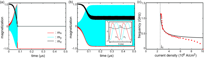
Figure 3: The time evolutions of $\mathbf{m}$ at $j=5.0\times 10^{6}$ A/cm² with $H_{\rm t}=5$ Oe for (a) $\mathbf{p}=+\mathbf{e}_{x}$ and (b) $\mathbf{p}=-\mathbf{e}_{x}$. The inset in (b) is an enlarged view. (c) The dependence of the oscillation frequency for $\mathbf{p}=-\mathbf{e}_{x}$ on the current density. The dots are obtained by the numerical simulation, while the solid line is obtained from Eqs. (12) and (13). It should be noted that these equations provide the relation between $f(E)$ and $j(E)$ above $j_{\rm c}$, which is $2.6\times 10^{6}$ A/cm² for $H_{\rm t}=5$ Oe.

IV Numerical Simulation

We confirm the validity of the above discussion by comparing with the numerical simulation. Figure 3 (a) shows an example of the time evolution of $\mathbf{m}$ when $\mathbf{p}=+\mathbf{e}_{x}$ obtained by numerically solving Eq. (1). The current density, $5.0\times 10^{6}$ A/cm², is larger than the critical current density, $2.2\times 10^{6}$ A/cm², estimated by Eq. (14). As shown, the magnetization finally stops at the film-plane, and does not show self-oscillation. We confirmed similar dynamics when $\mathbf{p}=-\mathbf{e}_{x}$, $H_{\rm t}>\widetilde{H}_{\rm t}$, and $|j|>|j_{\rm c}|$. These are consistent with the above discussions.

On the other hand, a stable self-oscillation is excited when $\mathbf{p}=-\mathbf{e}_{x}$ and $H_{\rm t}(=5\ {\rm Oe})<\widetilde{H}_{\rm t}$, as shown in Fig. 3 (b), where the current density is $5.0\times 10^{6}$ A/cm² while the critical current is $2.6\times 10^{6}$ A/cm². The dots in Fig. 3 (c) are the peak frequencies of the Fourier transformation of $m_{x}$, which is measured in experiment Kubota et al. (2013). The analytical estimation from Eqs. (12) and (13), shown by the solid line in Fig. 3 (c), works well in the relatively low current region, guaranteeing the validity of the theory. On the other hand, a discrepancy between the analytical and numerical results is found in the high current region due to the following reason. The theory assumes that the averaged work done by spin torque and dissipation due to damping during a precession are equal in the self-oscillation state. At each point on the constant energy curve however, the magnitudes of the spin torque and the damping torque are not equal because the spin torque and the damping torque have different angular dependences. When the spin torque (current) magnitude or the damping constant is large, a shift from the constant energy curve becomes large, and thus the magnetization cannot return to the constant energy curve during a precession. Then, the assumption in the averaged LLG equation does not stand, and the analytical theory is no more applicable to reproduce the numerical results. In fact, when the current density is $10\times 10^{6}$ A/cm², the magnetization does not show self-oscillation. In stead, it moves to $\mathbf{e}_{x}$ direction, and stops its dynamics because of the large spin torque strength. Therefore, the numerically obtained peak frequency in Fig. 3 (c) is zero.

V Discussion

The above analytical and numerical results show that a stable self-oscillation can be excited when a magnetic field smaller than Eq. (16) is applied anti-parallel to the magnetization of the pinned layer. The oscillation frequency changes continuously by increasing the current magnitude. The analytical relation between the current and frequency, obtained from Eqs. (12) and (13), works well in the low current region. In a high current region, the magnetization eventually arrives at the film-plane, and stops its dynamics. In this section, we compare these results with the previous works, and discuss the advantages to use the in-plane field.

Let us compare the present results with our previous work Taniguchi et al. (2013a), where the oscillation properties in the presence of a perpendicular field along the $z$-axis were studied. It was shown that, when the perpendicular field is smaller than $H_{\rm c}=[3\lambda^{2}/(2-3\lambda^{2})]H_{\rm K}^{\rm eff}$, the magnetization discontinuously moves from the perpendicular direction to a large cone angle by applying a current larger than the critical current. This discontinuous change of the cone angle significantly reduces the range of oscillation frequency in the self-oscillation state, as confirmed by experiment Tsunegi et al. (2014). Thus, a field larger than $H_{\rm c}$ should be applied to observe the oscillation in a wide range of the frequency Kubota et al. (2013); Taniguchi et al. (2013a). On the other hand, in the case of the in-plane field studied here, the cone angle of the magnetization continuously changes with the increase of the current. Therefore, a wide range of the oscillation frequency can be used. Also, the self-oscillation can be excited by a small field less than $\widetilde{H}_{\rm t}$ in Eq. (16), which is preferable from the view point of a low-power consumption. Therefore, the use of an in-plane magnetic field will be an important technical tool for piratical application.

The system studied above looks similar to an STO with the field-like torque Tulapurkar et al. (2005); Kubota et al. (2008); Sankey et al. (2008), which was studied in Ref. Taniguchi et al. (2014), because both the field-like torque and the torque due to the in-plane field point to $\mathbf{m}\times\mathbf{e}_{x}$ direction. However, there are important differences between these torques. The strength of the field-like torque depends on the electric current, and thus, the spin torque and the field-like torque cannot be manipulated independently. On the other hand, the magnitude of the in-plane field can be controlled independently from the spin torque. The sign of the field-like torque is determined by the material parameters and system size Tulapurkar et al. (2005); Kubota et al. (2008); Sankey et al. (2008); Zhang et al. (2002); Zwierzycki et al. (2005); Theodonis et al. (2006); Xiao and Bauer (2008), while the direction of the in-plane field is controllable. Regarding these points, the in-plane field is more convenient than the field-like torque to control self-oscillation, although the use of the field-like torque enables to excite self-oscillation without an external field.

Finally, we point out the importance of the parameter $\lambda$. The angular dependence of the spin torque, Eq. (7), characterized by $\lambda$, arises from the spin-dependent transport in a ferromagnetic multilayer. As can be seen from Eq. (7), the spin torque strength near the anti-parallel alignment of the magnetizations ($\mathbf{m}\simeq-\mathbf{p}$) is larger than that near the parallel alignment ($\mathbf{m}\simeq\mathbf{p}$). This is because, for example in a GMR system, the amount of the spin accumulation, which gives the spin torque on the magnetization, is large when the relative angle of the magnetizations is large. This parameter had been often neglected in previous works on, for example, an in-plane magnetized STO Pinna et al. (2014) because this angular dependence gives small corrections on the oscillation properties such as the critical current. However, the parameter $\lambda$ plays the dominant role in STO in which the constant energy curve is symmetric with respect to an axis perpendicular to the pinned layer magnetization Taniguchi (2014), as in the case of the present STO with a perpendicular field Taniguchi et al. (2013a). Although the constant energy curve in the this paper is asymmetric due to the in-plane field, this parameter still plays a key role to excite the oscillation. This is because the field $\tilde{H}_{\rm t}$ satisfies the following relation;

$$\lim_{\lambda\to 0}\tilde{H}_{\rm t}=0.$$ (17)

This indicates that the self-oscillation cannot be excited by an in-plane field when $\lambda=0$. In other words, a finite $\lambda$, which characterizes the asymmetry of the spin torque, is necessary to excite the self-oscillation. We notice that this conclusion is consistent with the previous study on an impossibility to excite self-oscillation by spin Hall effect Taniguchi (2015), where the spin Hall system corresponds to the limit of $\lambda\to 0$.

VI Conclusion

In summary, it was shown that a stable self-oscillation can be excited in an STO with a perpendicularly magnetized free layer and an in-plane magnetized pinned layer by applying a magnetic field smaller than a critical value, Eq. (16), pointing in the direction anti-parallel to the magnetization in the pinned layer. This is a preferable feature compared with the self-oscillation by a perpendicular field, in which relatively large field is necessary to stabilize the self-oscillation. The analytical relation between the current and the oscillation frequency was derived by solving the LLG equation. The comparison with numerical simulation shows that the theory works well in a low current region.

Appendix A Derivation of Eqs. (5) and (6)

The functions $\mathscr{W}_{\rm s}(E)$ and $\mathscr{W}_{\alpha}$, generally defined as

$$\mathscr{W}_{\rm s}(E)=\gamma M\oint dtH_{\rm s}\left[\mathbf{p}\cdot\mathbf{H}-\left(\mathbf{m}\cdot\mathbf{p}\right)\left(\mathbf{m}\cdot\mathbf{H}\right)\right],$$ (18)

$$\mathscr{W}_{\alpha}(E)=-\alpha\gamma M\oint dt\left[\mathbf{H}^{2}-\left(\mathbf{m}\cdot\mathbf{H}\right)^{2}\right],$$ (19)

are the work done by spin torque and the dissipation due to damping during a precession on a constant energy curve of $E$. The integral is over a precession period, given by Eq. (11), on the constant energy curve of $E$. Thus, the precession trajectory of the magnetization on the constant energy curve should be substituted into $\mathbf{m}$ in Eqs. (18) and (19). In the present system, such $\mathbf{m}$ is given by Taniguchi (2015)

$$m_{x}(E)=r_{3}+(r_{2}-r_{3}){\rm sn}^{2}(u,k),$$ (20)

$$m_{y}(E)=-(r_{2}-r_{3}){\rm sn}(u,k){\rm cn}(u,k)$$ (21)

$$m_{z}(E)=\sqrt{1-r_{3}^{2}-(r_{2}^{2}-r_{3}^{2}){\rm sn}^{2}(u,k)},$$ (22)

where $u=\gamma\sqrt{H_{\rm t}H_{\rm K}^{\rm eff}/2}\sqrt{r_{1}-r_{3}}t$, and $r_{\ell}$ are given by

$$r_{1}(E)=-\frac{E}{MH_{\rm t}},$$ (23)

$$r_{2}(E)=\frac{H_{\rm t}}{H_{\rm K}^{\rm eff}}+\sqrt{1+\left(\frac{H_{\rm t}}{H_{\rm K}^{\rm eff}}\right)^{2}+\frac{2E}{MH_{\rm K}^{\rm eff}}},$$ (24)

$$r_{3}(E)=\frac{H_{\rm t}}{H_{\rm K}^{\rm eff}}-\sqrt{1+\left(\frac{H_{\rm t}}{H_{\rm K}^{\rm eff}}\right)^{2}+\frac{2E}{MH_{\rm K}^{\rm eff}}},$$ (25)

The Jacobi elliptic functions, ${\rm sn}(u,k)$, ${\rm cn}(u,k)$, and ${\rm dn}(u,k)$ are useful to describe the precession trajectory. In the absence of the in-plane field, $H_{\rm t}=0$, the system shows the axial symmetry along the $z$-axis. In this case, the modulus $k$ becomes zero, and thus, the elliptic functions become trigonometric functions. Then, $\mathbf{m}$ in Eqs. (20), (21), and (22) become $m_{x}=-\sin\theta\cos\omega t$, $m_{y}=-\sin\theta\sin\omega t$, and $m_{z}=\cos\theta$, where $\theta$ is a constant and $\omega=\gamma H_{\rm K}^{\rm eff}\cos\theta$. This solution describes circular motion of the magnetization around the $z$-axis with the initial condition $m_{x}(0)=-\sin\theta$.

Substituting Eqs. (20), (21), and (22) into Eqs. (18) and (19), we obtain Eqs. (5) and (6). The explicit form of the integral of Eq. (5) for $\mathbf{p}=+\mathbf{e}_{x}$ is given by

$$\begin{split}\mathscr{W}_{\rm s}=\frac{\gamma\hbar\eta j}{2ed}&\int_{0}^{\tau}dt\left\{\frac{H_{\rm t}(1-\lambda r_{3})-H_{\rm K}^{\rm eff}[r_{2}+r_{3}+\lambda(1-r_{3}^{2})]}{\lambda^{2}}\right.\\ &-\frac{H_{\rm t}(r_{2}-r_{3})-H_{\rm K}^{\rm eff}(r_{2}^{2}-r_{3}^{2})}{\lambda}{\rm sn}^{2}(u,k)\\ &-\left.\frac{H_{\rm t}(1-\lambda^{2})-H_{\rm K}^{\rm eff}[r_{2}+r_{3}+\lambda(1+r_{2}r_{3})]}{\lambda^{2}[1+\lambda r_{3}+\lambda(r_{2}-r_{3}){\rm sn}^{2}(u,k)]}\right\},\end{split}$$ (26)

while that of Eq. (6) is shown in Ref. Taniguchi (2015). The explicit form of $\mathscr{W}_{\rm s}$ for $\mathbf{p}=-\mathbf{e}_{x}$ is obtained by replacing $\lambda$ with $-\lambda$ and multiplying a minus sign in whole. Then, Eqs. (5) and (6) are derived by using the following integral formulas Byrd and Friedman (1971);

$$\int^{u}du^{\prime}{\rm sn}^{2}(u^{\prime},k)=\frac{\mathsf{F}[{\rm am}(u,k),k]-\mathsf{E}[{\rm am}(u,k),k]}{k^{2}},$$ (27)

$$\begin{split}\int^{u}du^{\prime}{\rm sn}^{4}(u^{\prime},k)=&\frac{{\rm sn}(u,k){\rm cn}(u,k){\rm dn}(u,k)}{3k^{2}}\\ &+\frac{2+k^{2}}{3k^{4}}\mathsf{F}[{\rm am}(u,k),k]\\ &-\frac{2(1+k^{2})}{3k^{4}}\mathsf{E}[{\rm am}(u,k),k],\end{split}$$ (28)

$$\int^{u}\frac{du^{\prime}}{b+a{\rm sn}^{2}(u^{\prime},k)}=\frac{1}{b}\Pi[{\rm am}(u,k),k,-a/b],$$ (29)

where

$$\mathsf{F}(\varphi,k)=\int_{0}^{\varphi}\frac{d\varphi^{\prime}}{\sqrt{1-k^{2}\sin^{2}\varphi^{\prime}}},$$ (30)

$$\mathsf{E}(\varphi,k)=\int_{0}^{\varphi}d\varphi^{\prime}\sqrt{1-k^{2}\sin^{2}\varphi^{\prime}},$$ (31)

$$\Pi(\varphi,k,n)=\int_{0}^{\varphi}\frac{d\varphi^{\prime}}{(1-n\sin^{2}\varphi^{\prime})\sqrt{1-k^{2}\sin^{2}\varphi^{\prime}}}.$$ (32)

are the first, second, and third kind of incomplete elliptic integrals, respectively. The Jacobi amplitude function is denoted as ${\rm am}(u,k)$. We note that $\mathsf{F}[{\rm am}(u,k),k]=u$, $\mathsf{E}[{\rm am}(\mathsf{K}(k),k),k]=\mathsf{E}(k)$, and $\Pi[{\rm am}(\mathsf{K}(k),k),k,n]=\Pi(k,n)$, where the first, second, and third kind of complete integrals are defined as $\mathsf{K}(k)=\mathsf{F}(\pi/2,k)$, $\mathsf{E}(k)=\mathsf{E}(\pi/2,k)$, and $\Pi(k,n)=\Pi(\pi/2,k,n)$, respectively.

References

- Slonczewski (1996) J. C. Slonczewski, J. Magn. Magn. Mater. 159, L1 (1996).
- Berger (1996) L. Berger, Phys. Rev. B 54, 9353 (1996).
- Kiselev et al. (2003) S. I. Kiselev, J. C. Sankey, I. N. Krivorotov, N. C. Emley, R. J. Schoelkopf, R. A. Buhrman, and D. C. Ralph, Nature 425, 380 (2003).
- Rippard et al. (2004) W. H. Rippard, M. R. Pufall, S. Kaka, S. E. Russek, and T. J. Silva, Phys. Rev. Lett. 92, 027201 (2004).
- Houssameddine et al. (2007) D. Houssameddine, U. Ebels, B. Delaët, B. Rodmacq, I. Firastrau, F. Ponthenier, M. Brunet, C. Thirion, J.-P. Michel, L. Prejbeanu-Buda, et al., Nat. Mater. 6, 447 (2007).
- Pribiag et al. (2007) V. S. Pribiag, I. N. Krivorotov, G. D. Fuchs, P. M. Braganca, O. Ozatay, J. C. Sankey, D. C. Ralph, and R. A. Buhrman, Nat. Phys. 3, 498 (2007).
- Mistral et al. (2008) Q. Mistral, M. van Kampen, G. Hrkac, J.-V. Kim, T. Devolder, P. Crozat, C. Chappert, L. Lagae, and T. Schrefl, Phys. Rev. Lett. 100, 257201 (2008).
- Kudo et al. (2009) K. Kudo, T. Nagasawa, R. Sato, and K. Mizushima, Appl. Phys. Lett. 95, 022507 (2009).
- Dussaux et al. (2010) A. Dussaux, B. Georges, J. Grollier, V. Cros, A. V. Khavalkovskiy, A. Fukushima, M. Konoto, H. Kubota, K. Yakushiji, S. Yuasa, et al., Nat. Commun. 1, 8 (2010).
- Zeng et al. (2012) Z. Zeng, P. K. Amiri, I. Krivorotov, H. Zhao, G. Finocchio, J.-P. Wang, J. A. Katine, Y. Huai, J. Langer, K. Galatsis, et al., ACS Nano 6, 6115 (2012).
- Kubota et al. (2013) H. Kubota, K. Yakushiji, A. Fukushima, S. Tamaru, M. Konoto, T. Nozaki, S. Ishibashi, T. Saruya, S. Yuasa, T. Taniguchi, et al., Appl. Phys. Express 6, 103003 (2013).
- Lebrun et al. (2014) R. Lebrun, N. Locatelli, S. Tsunegi, J. Grollier, V. Cros, F. A. Araujo, H. Kubota, K. Yakushiji, A. Fukushima, and S. Yuasa, Phys. Rev. Applied 2, 061001 (2014).
- Yakata et al. (2009) S. Yakata, H. Kubota, Y. Suzuki, K. Yakushiji, A. Fukushima, S. Yuasa, and K. Ando, J. Appl. Phys. 105, 07D131 (2009).
- Ikeda et al. (2010) S. Ikeda, K. Miura, H. Yamamoto, K. Mizunuma, H. D. Gan, M. Endo, S. Kanai, J. Hayakawa, F. Matsukura, and H. Ohno, Nat. Mater. 9, 721 (2010).
- Kubota et al. (2012) H. Kubota, S. Ishibashi, T. Saruya, T. Nozaki, A. Fukushima, K. Yakushiji, K. Ando, Y. Suzuki, and S. Yuasa, J. Appl. Phys. 111, 07C723 (2012).
- Bertotti et al. (2009) G. Bertotti, I. Mayergoyz, and C. Serpico, Nonlinear magnetization Dynamics in Nanosystems (Elsevier, Oxford, 2009), chap. 9.
- Ebels et al. (2008) U. Ebels, D. Houssameddine, I. Firastrau, D. Gusakova, C. Thirion, B. Dieny, and L. D. Buda-Prejbeanu, Phys. Rev. B 78, 024436 (2008).
- Silva and Keller (2010) T. J. Silva and M. W. Keller, IEEE Trans. Magn. 46, 3555 (2010).
- Gusakova et al. (2011) D. Gusakova, M. Quinsat, J. F. Sierra, U. Ebels, B. Dieny, and L. D. Buda-Prejbeanu, Appl. Phys. Lett. 99, 052501 (2011).
- Khalsa et al. (2015) G. Khalsa, M. D. Stiles, and J. Grollier, Appl. Phys. Lett. 106, 242402 (2015).
- Taniguchi et al. (2013a) T. Taniguchi, H. Arai, S. Tsunegi, S. Tamaru, H. Kubota, and H. Imamura, Appl. Phys. Express 6, 123003 (2013a).
- Taniguchi (2014) T. Taniguchi, Appl. Phys. Express 7, 053004 (2014).
- Pinna et al. (2014) D. Pinna, D. L. Stein, and A. D. Kent, Phys. Rev. B 90, 174405 (2014).
- Taniguchi (2015) T. Taniguchi, Phys. Rev. B 91, 104406 (2015).
- Slavin and Tiberkevich (2009) A. Slavin and V. Tiberkevich, IEEE. Trans. Magn. 45, 1875 (2009).
- Kim (2012) J.-V. Kim, Sol. Stat. Phys. 63, 217 (2012).
- Oogane et al. (2006) M. Oogane, T. Wakitani, S. Yakata, R. Yilgin, Y. Ando, A. Sakuma, and T. Miyazaki, Jpn. J. Appl. Phys. 45, 3889 (2006).
- Konoto et al. (2013) M. Konoto, H. Imamura, T. Taniguchi, K. Yakushiji, H. Kubota, A. Fukushima, K. Ando, and S. Yuasa, Appl. Phys. Express 6, 073002 (2013).
- Iihama et al. (2014) S. Iihama, S. Mizukami, H. Naganuma, M. Oogane, Y. Ando, and T. Miyazaki, Phys. Rev. B 89, 174416 (2014).
- Slonczewski (1989) J. C. Slonczewski, Phys. Rev. B 39, 6995 (1989).
- Slonczewski (2005) J. C. Slonczewski, Phys. Rev. B 71, 024411 (2005).
- Xiao et al. (2004) J. Xiao, A. Zhangwill, and M. D. Stiles, Phys. Rev. B 70, 172405 (2004).
- Bertotti et al. (2004) G. Bertotti, I. D. Mayergoyz, and C. Serpico, J. Appl. Phys. 95, 6598 (2004).
- Bertotti et al. (2006) G. Bertotti, I. D. Mayergoyz, and C. Serpico, J. Appl. Phys. 99, 08F301 (2006).
- Serpico et al. (2005) C. Serpico, M. d’Aquino, G. Bertotti, and I. D. Mayergoyz, J. Magn. Magn. Mater. 290, 502 (2005).
- Apalkov and Visscher (2005) D. M. Apalkov and P. B. Visscher, Phys. Rev. B 72, 180405 (2005).
- Hillebrands and Thiaville (2006) B. Hillebrands and A. Thiaville, eds., Spin Dynamics in Confined Magnetic Structures III (Springer, Berlin, 2006).
- Dykman (2012) M. Dykman, ed., Fluctuating Nonlinear Oscillators (Oxford University Press, Oxford, 2012), chap. 6.
- Newhall and Eijnden (2013) K. A. Newhall and E. V. Eijnden, J. Appl. Phys. 113, 184105 (2013).
- Taniguchi et al. (2013b) T. Taniguchi, Y. Utsumi, M. Marthaler, D. S. Golubev, and H. Imamura, Phys. Rev. B 87, 054406 (2013b).
- Tsunegi et al. (2014) S. Tsunegi, T. Taniguchi, H. Kubota, H. Imamura, S. Tamaru, M. Konoto, K. Yakushiji, A. Fukushima, and S. Yuasa, Jpn. J. Appl. Phys. 53, 060307 (2014).
- Tulapurkar et al. (2005) A. A. Tulapurkar, Y. Suzuki, A. Fukushima, H. Kubota, H. Maehara, K. Tsunekawa, D. D. Djayaprawira, N. Watanabe, and S. Yuasa, Nature 438, 339 (2005).
- Kubota et al. (2008) H. Kubota, A. Fukushima, K. Yakushiji, T. Nagahama, S. Yuasa, K. Ando, H. Maehara, Y. Nagamine, K. Tsunekawa, D. D. Djayaprawira, et al., Nat. Phys. 4, 37 (2008).
- Sankey et al. (2008) J. C. Sankey, Y.-T. Cui, J. Z. Sun, J. C. Slonczewski, R. A. Buhrman, and D. C. Ralph, Nat. Phys. 4, 67 (2008).
- Taniguchi et al. (2014) T. Taniguchi, S. Tsunegi, H. Kubota, and H. Imamura, Appl. Phys. Lett. 104, 152411 (2014).
- Zhang et al. (2002) S. Zhang, P. M. Levy, and A. Fert, Phys. Rev. Lett. 88, 236601 (2002).
- Zwierzycki et al. (2005) M. Zwierzycki, Y. Tserkovnyak, P. J. Kelly, A. Brataas, and G. E. W. Bauer, Phys. Rev. B 71, 064420 (2005).
- Theodonis et al. (2006) I. Theodonis, N. Kioussis, A. Kalitsov, M. Chshiev, and W. H. Butler, Phys. Rev. Lett. 97, 237205 (2006).
- Xiao and Bauer (2008) J. Xiao and G. E. W. Bauer, Phys. Rev. B 77, 224419 (2008).
- Byrd and Friedman (1971) P. F. Byrd and M. D. Friedman, Handbook of Elliptic Integrals for Engineers and Scientists (Springer, 1971), 2nd ed.