Mean field approximation of many-body quantum dynamics for Bosons in a discrete numerical model

Abstract

The mean field approximation is numerically validated in the bosonic case by considering the time evolution of quantum states and their associated reduced density matrices by many-body Schrödinger dynamics. The model phase-space is finite-dimensional. The results are illustrated with numerical simulations of the evolution of quantum states according to the time, the number of the particles, and the dimension of the phase-space.

Mathematics subject classification: 81S30, 81S05, 81T10, 35Q55, 81P40
Keywords: mean field limit, reduced density matrices, Wigner measures, bosons Fock space, second quantization.

1 Introduction

The mean field approximation is known to be a good way to approximate the many-body Schrödinger dynamics when the number of particles is large enough (see [2, 6, 9, 10, 15, 19, 20, 21, 22, 24, 25, 26, 32, 37, 43, 46, 29, 30, 33, 50]).
It consists in looking for the solutions to the non-linear Schrödinger equation for one particle called the Hartree equation. We are interested in the density matrix associated with the wave function, this matrix satisfies the quantum Liouville equation dual to the Von Neumann equation.The partial trace operators of this matrix, called the reduced density matrices, satisfy a hierarchy of equations. For instance, by considering the case where the initial state for the Schrödinger equation is a Hartree ansatz(a product state) which is suitable for a bosons condensate, the limit, when the number of particles $N$ goes to the infinity of these matrices converge in trace norm to the product of the density matrix associated with the solution to the Hartree equation. And this asymptotic density matrix satisfies the time dependent Hartree equation [8].
When the particles are bosons, the suitable space for the bosons is the symmetric Fock space on the phase-space. Moreover for the sake of numerical computations, a finite-dimensional phase-space will be used instead of an usual phase-space of type $L^{2}(\mathbb{R}^{d})$. So here the phase-space will be $\mathcal{Z}=\ell^{2}(\{0,\cdots,K\})\simeq\mathbb{C}^{K}$ where $K$ is a given integer representing the number of sites. Each particle can live in one of the $K$ sites.
For the numerical implementation, an explicit basis of the $N$-fold sector of the Fock bosonic spaces is specified. This basis allows the numerical computation of the full $N$-body quantum problem for $N$ large enough to validate various mean field regimes, in spite of a rapidly increasing complexity.
The resolution of the $N$-particles Schrödinger equation will rely on a splitting method, one part for the free Hamiltonian and the other one for the two particles interaction term.
For the simulations, the considered real bounded potential associated with the interaction term will be $V$ defined on $\mathbb{Z}/K\mathbb{Z}$ by $V(i)=\frac{1}{|i|}$ if $i\neq 0$ and $V(0)=0$.
According to previous results related to the propagation of the Wigner measures [3, 4, 5, 6] knowing the Wigner measure at time $t=0$ determines the Wigner measure at time $t$ and all asymptotic reduced density matrices. For many examples, like Hermite states, twin Fock states or states studied in quantum information theory (see [1]) their Wigner measure as well as the order of convergence of reduced density matrices is known explicitly. The evolution of the Wigner measure, and consequently of the asymptotic density matrices, is evaluated after integrating numerically the mean field non linear Hartree time-dependent equation. In order to preserve numerically quadratic quantities like the symplectic form, the latter is solved with a symplectic $4^{th}$ order Runge-Kutta method ([35]).
To estimate numerically the error of convergence of the reduced density matrices in the mean field limit, a discretization of a time interval $[0,t_{max}]$ is considered, in the examples $t_{max}=1$ is chosen, then the quantity $\max_{t\in[0,t_{max}]}\left\|\gamma^{(p)}_{N}(t)-\gamma_{\infty}^{(p)}(t)\right\|_{1}$ is observed. Here $\gamma^{(p)}_{N}(t)$ denotes the time-evolved $p$ particles reduced density matrix for $N$ bosons, while $\gamma_{\infty}^{(p)}(t)$ is its theoretical limit when $N$ goes to the infinity, and $\|.\|_{1}$ denoting the trace norm.
For the evaluation of the order of convergence, the logarithm of the previous error estimate is drawn according to $log(N)$. This gives a straight line whose the slope is the order of convergence in $1/N$.
These numerical results agree very well and illustrate the theoretical analysis carried out in [1].
By increasing $K$, we wish to approach a continuous model. The complexity of the computations increase in the same time that $K$ and $N$ increase because of the dimension of the $N$-particles bosons Fock space on $\mathbb{C}^{K}$ which is a binomial coefficient.

2 Framework

The bosons Fock space on an Hilbert space $\mathcal{Z}$ is defined as $\Gamma_{s}(\mathcal{Z})=\bigoplus_{n\geq 0}\bigvee^{n}\mathcal{Z}$ where $\bigvee^{n}\mathcal{Z}$ is the symmetric n-fold Hilbertian tensor product of $\mathcal{Z}$ which is the range of the projection defined on the Hilbert tensor product $\mathcal{Z}^{\otimes n}$, by:

$$S_{n}(\xi_{1}\otimes\xi_{2}\otimes...\otimes\xi_{n})=\frac{1}{n!}\sum_{\sigma\in\Sigma_{n}}\xi_{\sigma(1)}\otimes\xi_{\sigma(2)}\otimes...\otimes\xi_{\sigma(n)},$$

where $\xi_{i}$ is in $\mathcal{Z}$ for each $i$ in $[1,n]$ and $\Sigma_{n}$ is the set of the permutations of $n$ elements.

For $z$ in $\mathcal{Z}$ and $\varepsilon$ positive, the $\varepsilon$-scaled annihilation and creation operators are defined for all $\Phi$ in $\mathcal{Z}$ and $n$ in $\mathbb{N}$ by:

$$a(z)\Phi^{\otimes n} =\sqrt{\varepsilon n}\langle z|\Phi\rangle\Phi^{\otimes n-1},$$

$$a^{*}(z)\Phi^{\otimes n} =\sqrt{\varepsilon(n+1)}S_{n+1}(|z\rangle\otimes\Phi^{\otimes n}).$$

These operators are then extended by linearity and density to $\bigvee^{n}\mathcal{Z}$.

These operators satisfy the canonical commutation relations (CCR):

$$[a(z_{1}),a^{*}(z_{2})] =\varepsilon\langle z_{1},z_{2}\rangle Id\;,$$ (1)

$$[a(z_{1}),a(z_{2})] =0\;,$$ (2)

$$[a^{*}(z_{1}),a^{*}(z_{2})] =0\;.$$ (3)

The second quantization of an operator $A\in\mathcal{L}(\mathcal{Z})$ or a self-adjoint operator $(A,D(A))$ in $\mathcal{Z}$ is defined by:

$$d\Gamma(A)_{|\vee^{n,alg}D(A)}=\varepsilon\sum_{i=1}^{n}Id^{\otimes i-1}\otimes A\otimes Id^{\otimes n-i}\;.$$

The second quantization of $Id_{\mathcal{Z}}$ is the number operator:

$$\mathbf{N}_{|\vee^{n}\mathcal{Z}}=\varepsilon nId_{\vee^{n}\mathcal{Z}}\;.$$

2.1 Orthogonal basis of the $N$-fold sector

Use the following notations: $\mathbb{Z}_{K}=\mathbb{Z}/K\mathbb{Z}\;.$
For $\alpha=(\alpha_{1},\cdots,\alpha_{K})$ in $\mathbb{N}^{K}$, the length of $\alpha$ is written $|\alpha|=\alpha_{1}+\cdots+\alpha_{K}$ and the factorial of $\alpha$ $\alpha!=\alpha_{1}!\cdots\alpha_{K}!\;.$
Let $(e_{1},\cdots,e_{K})$ be an orthonormal basis of $\mathbb{C}^{K}$.
Set $\mathcal{Z}=\mathbb{C}^{K}$. Then an orthonormal basis of $\bigvee^{N}\mathcal{Z}$ can be built from this basis which is labelled by the multi-indices $\alpha$ in $\mathbb{N}^{K}$ such that $|\alpha|=N$.

With the creation operators, an orthonormal basis can be written as:

$$e_{\alpha}:=\frac{a^{*}(e)^{\alpha}}{\sqrt{\varepsilon^{|\alpha|}\alpha!}}|\Omega\rangle:=\frac{1}{\sqrt{\varepsilon^{|\alpha|}\alpha!}}a^{*}(e_{1})^{\alpha_{1}}\cdots{a^{*}(e_{K})}^{\alpha_{K}}|\Omega\rangle\,,$$

where $|\Omega\rangle=(1,0,0,0,\ldots)$ is the vacuum of the Fock space.

Then the dimension of $\bigvee^{N}\mathcal{Z}$ is $card(\{\alpha\in\mathbb{N}^{K}/|\alpha|=N\})=\dbinom{N+K-1}{K-1}\;.$
And $card(\{\alpha\in\mathbb{N}^{K}/|\alpha|\leq N\})={N+K\choose K}$ is the dimension of $\bigoplus_{n=0}^{N}\bigvee^{n}\mathcal{Z}\;.$

2.2 Hamiltonian

As a binomial number, the dimension of the $N$ particles bosonic sector increases rapidly but not too much, as $N$ increases (see Table Appendix for numerical values).The complexity has to be handled carefully if we want to approach the mean field limit by taking $N$ large or the continuous model by taking $K$ large.
Define $\Delta_{K}$ the discrete Laplacian operator on $\mathbb{C}^{K}$ by:

$$\forall z\in\mathbb{C}^{K}\;\;,\quad\forall i\in\mathbb{Z}/K\mathbb{Z},\quad(\Delta_{K}z)_{i}=z_{i+1}+z_{i-1}\;.$$

And let $H_{0}=d\Gamma(-\Delta_{K})$ be the free Hamiltonian.

The interaction term denoted by $\mathcal{V}$ equals:

$$\mathcal{V}=\frac{1}{2}\sum_{(i,j)\in\mathbb{Z}_{K}^{2}}V_{ij}a^{*}(e_{i})a^{*}(e_{j})a(e_{i})a(e_{j})\;,$$

where $V_{ij}=V_{ji}=V(i-j)$.
In this framework changing the value of $V(0)$ add an irrelevant phase factor in the time evolved wave function. In the sequel $V(0)=0$ is assumed.
Or as a Wick quantized operator (14):

$$\mathcal{V}=\big{\langle}z^{\otimes 2},\big{(}\frac{1}{2}\sum_{(i,j)\in\mathbb{Z}_{K}^{2}}V_{ij}|e_{i}\otimes e_{j}\rangle\langle e_{i}\otimes e_{j}|\big{)}z^{\otimes 2}\big{\rangle}^{Wick}\;.$$

The considered linear Schrödinger equation is:

$$\mathrm{i}\varepsilon\partial_{t}\Psi=H_{\varepsilon}\Psi\;,$$ (4)

where the complete Hamiltonian is defined on the bosonic Fock space by :

$$H_{\varepsilon}=d\Gamma(-\Delta_{K})+\mathcal{V}\;.$$

3 Finite dimensional mean field equation

3.1 Energy of the Hamiltonian

The energy of the Hamiltonian corresponds to the symbol of the complete Hamiltonian:

$$H(z,\bar{z})=\langle z,-\Delta_{K}z\rangle+\frac{1}{2}\sum_{i\neq j}V_{ij}|z_{i}|^{2}|z_{j}|^{2}\;,$$

while recalling our convention $V_{ii}=V(0)=0$ for all $i$ in $\mathbb{Z}_{K}$.

3.2 Hartree equation

The mean field equation in $\mathcal{Z}$ is written as:

$$\mathrm{i}\partial_{t}z=\partial_{\bar{z}}H(z,\bar{z})\;.$$

For each component in $\mathbb{C}^{K}$ we obtain:

$$\mathrm{i}\partial_{t}z_{i} =\partial_{\bar{z}_{i}}H=\partial_{\bar{z}_{i}}(\sum_{i^{\prime}}|z_{i^{\prime}}-z_{i^{\prime}-1}|^{2}-2|z_{i}|^{2}+\frac{1}{2}\sum_{i^{\prime}\neq j}V_{i^{\prime}j}|z_{i^{\prime}}|^{2}|z_{j}|^{2})$$

$$=\partial_{\bar{z}_{i}}(\sum_{i^{\prime}}(\bar{z_{i^{\prime}}}-\bar{z_{i^{\prime}-1}})(z_{i^{\prime}}-z_{i^{\prime}-1})-2\bar{z_{i}}z_{i}+\frac{1}{2}\sum_{i^{\prime}\neq j}V_{i^{\prime}j}\bar{z_{i^{\prime}}}z_{i^{\prime}}\bar{z_{j}}z_{j})$$

$$=z_{i}-z_{i-1}-(z_{i+1}-z_{i})-2z_{i}+\sum_{j\neq i}V_{ij}z_{i}|z_{j}|^{2}$$

$$=-(z_{i+1}+z_{i-1})+(\sum_{j\neq i}V_{ij}|z_{j}|^{2})z_{i}$$

$$\dot{z}_{i}=-\mathrm{i}[-(\Delta_{K}z)_{i}+(\sum_{j\neq i}V_{ij}|z_{j}|^{2})z_{i}]$$

By writing $z=q+\mathrm{i}p$ where $q$ and $p$ belong to $\mathbb{R}^{K}$, it becomes:

$$\dot{q}_{i} = -(p_{i+1}+p_{i-1})+\sum_{j\neq i}V_{ij}(q_{j}^{2}+p_{j}^{2})p_{i}$$

$$\dot{p}_{i} = -\Big{(}-(q_{i+1}+q_{i-1})+\sum_{j\neq i}V_{ij}(q_{j}^{2}+p_{j}^{2})q_{i}\Big{)}$$

A $4^{th}$ or $6^{th}$ order Gauss RK method is used by using the coefficients given in [35] to solve the Hartree equation.
A symplectic method is used to preserve the quadratic part of the energy, the symplectic form and the phase space volume.

3.3 Wigner measures

For $f\in\mathcal{Z}$ the field operator is defined by $\Phi(f)=\frac{1}{\sqrt{2}}(a^{*}(f)+a(f))$ which is essentially self-adjoint on $\Gamma_{fin}(\mathcal{Z})=\bigoplus_{n\in\mathbb{N}}^{alg}\bigvee^{n}\mathcal{Z}$
The Weyl operator is defined by $W(f)=e^{i\Phi(f)}$.

Let $(\varrho_{\varepsilon})_{\varepsilon\in\mathcal{E}}$ be a family of normal states on $\Gamma_{z}(\mathcal{Z})$ with $\mathcal{E}\subset(0,+\infty)$, $0\in\overline{\mathcal{E}}$.
A measure $\mu$ is a Wigner measure for this family, $\mu\in\mathcal{M}(\varrho_{\varepsilon},\varepsilon\in\mathcal{E})$, if there exists $\mathcal{E}^{\prime}\subset\mathcal{E}$, $0\in\overline{\mathcal{E}^{\prime}}$ such that

$$\forall f\in\mathcal{Z}\,,\lim_{\varepsilon\in\mathcal{E}^{\prime}\,,\varepsilon\to 0}{\rm{Tr}}\left[\varrho_{\varepsilon}W(\sqrt{2}\pi f)\right]=\int_{\mathcal{Z}}e^{2i\pi\textrm{Re}~{}\langle f,z\rangle}~{}d\mu(z)\;,$$

see [42].
The following result valid for separable Hilbert spaces $\mathcal{Z}$, apply to our finite dimensional $\mathcal{Z}\simeq\mathbb{C}^{K}$.

Theorem 3.1

[3]. If $(\varrho_{\varepsilon})_{\varepsilon\in\mathcal{E}}$ satisfies the uniform estimate ${\rm{Tr}}[\varrho_{\varepsilon}\mathbf{N}^{\delta}]\leq{C_{\delta}}<+\infty$ for some $\delta>0$ fixed, $\mathcal{M}(\varrho_{\varepsilon},\varepsilon\in\mathcal{E})$ is not empty and made of Borel probability measures ($\mathcal{Z}$ separable) such that $\int_{\mathcal{Z}}|z|^{2\delta}d\mu(z)\leq C_{\delta}$.

For each $p$ in $\mathbb{N}$, the reduced density matrix associated with a state $\varrho_{\varepsilon}$ is a trace class operator in $\mathcal{L}^{1}(\bigvee^{p}\mathcal{Z})$ defined by the duality relation:

$${\rm{Tr}}\left[\gamma_{\varepsilon}^{p}\tilde{b}\right]=\frac{{\rm{Tr}}\left[\varrho_{\varepsilon}b^{Wick}\right]}{{\rm{Tr}}\left[\varrho_{\varepsilon}(|z|^{2p})^{Wick}\right]}$$ (5)

where $\tilde{b}\in\mathcal{L}(\bigvee^{p}\mathcal{Z})$.
The asymptotic reduced density matrix associated with the Wigner measure $\mu$ equals:

$$\gamma_{0}^{p}=\frac{\int_{\mathcal{Z}}|z^{\otimes p}\rangle\langle z^{\otimes p}|d\mu(z)}{\int_{\mathcal{Z}}|z|^{2p}d\mu(z)}\,.$$ (6)

In finite dimension, if the family $(\varrho_{\varepsilon})_{\varepsilon\in\mathcal{E}}$ satisfies $\mathcal{M}(\varrho_{\varepsilon},\varepsilon\in\mathcal{E})=\left\{\mu\right\}$ then the $(PI)$-condition (see [3]):

$$\forall p\in\mathbb{N}\,,\lim_{\varepsilon\in\mathcal{E},\varepsilon\to 0}{\rm{Tr}}\left[\varrho_{\varepsilon}\mathbf{N}^{p}\right]=\int_{\mathcal{Z}}|z|^{2p}~{}d\mu(z)\,$$

is always satisfied.

3.4 Reduced density matrices

Theorem 3.2

[5]. If the family $(\varrho_{\varepsilon})_{\varepsilon\in\mathcal{E}}$ satisfies $\mathcal{M}(\varrho_{\varepsilon},\varepsilon\in\mathcal{E})=\left\{\mu\right\}$ with the $(PI)$-condition:

$$\forall p\in\mathbb{N}\,,\lim_{\varepsilon\in\mathcal{E},\varepsilon\to 0}{\rm{Tr}}\left[\varrho_{\varepsilon}\mathbf{N}^{p}\right]=\int_{\mathcal{Z}}|z|^{2p}~{}d\mu(z)\;,$$

then ${\rm{Tr}}\left[\varrho_{\varepsilon}b^{Wick}\right]$ converges to $\int_{\mathcal{Z}}b(z)~{}d\mu(z)$ for all polynomial $b(z)$ and

$$\lim_{\varepsilon\in\mathcal{E}\,,\varepsilon\to 0}\|\gamma_{\varepsilon}^{p}-\gamma_{0}^{p}\|_{\mathcal{L}^{1}}=0$$

for all $p\in\mathbb{N}$.

Theorem 3.3

[5, 6, 42]. Assume $\mathcal{M}(\varrho_{\varepsilon},\varepsilon\in(0,\bar{\varepsilon})=\left\{\mu_{0}\right\}$ and the condition $(PI)$ . Then $\mathcal{M}(e^{-i\frac{t}{\varepsilon}H_{\varepsilon}}\varrho_{\varepsilon}e^{i\frac{t}{\varepsilon}H_{\varepsilon}},\varepsilon\in(0,\bar{\varepsilon}))=\left\{\mu_{t}\right\}$. The measure $\mu_{t}=\Phi(t,0)_{*}\mu_{0}$ is the push-forward measure of the initial measure $\mu_{0}$ where $\Phi(t,0)$ is the hamiltonian flow associated with the equation

$$i\partial_{t}z_{k}(t)=-\Delta_{K}z_{k}(t)+\sum_{j}V_{kj}|z_{j}|^{2}z_{k}\,.$$ (7)

After propagation of the Wigner measures, for any $p\in\mathbb{N}$, the convergence of the reduced densiy matrices is obtained at any time $t$:

$$\Big{\|}\gamma_{\varepsilon}^{p}(t)-\frac{\int_{\mathcal{Z}}|z^{\otimes p}\rangle\langle z^{\otimes p}|d\mu_{t}(z)}{\int_{\mathcal{Z}}|z|^{2p}d\mu_{0}(z)}\Big{\|}_{\mathcal{L}^{1}}\longrightarrow 0.$$

Theorem 3.4

[1]. Let $(\alpha(n))_{n\in\mathbb{N}^{*}}$ be a sequence of positive numbers with $\lim\alpha(n)=\infty$ and such that $(\frac{\alpha(n)}{n})_{n\in\mathbb{N}^{*}}$ is bounded. Let $(\varrho_{n})_{n\in\mathbb{N}^{*}}$ and $(\gamma_{\infty}^{(p)})_{p\in\mathbb{N}^{*}}$ be two sequences of density matrices with $\varrho_{n}\in{\mathscr{L}}^{1}(\bigvee^{n}\mathcal{Z})$ and $\gamma_{\infty}^{(p)}\in{\mathscr{L}}^{1}(\bigvee^{p}\mathcal{Z})$ for each $n,p\in\mathbb{N}^{*}$. Assume that there exist $C_{0}>0$, $C>2$ and $\gamma\geq 1$ such that for all $n,p\in\mathbb{N}^{*}$ with $n\geq\gamma p$:

$$\left\|\gamma^{(p)}_{n}-\gamma_{\infty}^{(p)}\right\|_{1}\leq C_{0}\frac{C^{p}}{\alpha(n)}\,.$$ (8)

Then for any $T>0$ there exists $C_{T}>0$ such that for all $t\in[-T,T]$ and all $n,p\in\mathbb{N}^{*}$ with $n\geq\gamma p$,

$$\left\|\gamma^{(p)}_{n}(t)-\gamma_{\infty}^{(p)}(t)\right\|_{1}\leq C_{T}\frac{C^{p}}{\alpha(n)}\,,$$ (9)

where

$$\gamma_{\infty}^{(p)}(t)=\int_{\mathcal{Z}}|z^{\otimes p}\rangle\langle z^{\otimes p}|\,d\mu_{t}(z)\,,$$

with $\mu_{t}=(\Phi_{t})_{\sharp}\mu_{0}$ is the push-forward of the initial measure $\mu_{0}$ by the well defined and continuous Hartree flow $\Phi_{t}$ on $\mathcal{Z}$.

4 Numerical methods

4.1 Method to solve the Hartree equation

To solve the mean field equation (7), a Runge-Kutta method is used.

Let $b_{i}$, $a_{ij}$ $(i,j=1,\ldots,s)$ be real numbers and $c_{i}=\sum_{j=1}^{s}a_{ij}$.
An s-stage Runge-Kutta method with a time step $h$ to solve a first-order ordinary equation $y^{\prime}=f(t,y)$ , $y(t_{0})=y_{0}$ is given by:

$$k_{i} = f(t_{0}+c_{i}h,y_{0}+h\sum_{j=1}^{s}a_{ij}k_{j})\;,i=1,\ldots,s$$

$$y_{1} = y_{0}+h\sum_{i=1}^{s}b_{i}k_{i}$$

represented as:

$c_{1}$	$a_{11}$	…	$a_{1s}$
⋮	⋮		⋮
$c_{s}$	$a_{s1}$	$\ldots$	$a_{ss}$
	$b_{1}$	…	$b_{s}$

.

Here the system is autonomous, and according to [35] the coefficients used for the Gauss RK method are:
0 1/2 1/2 1/2 0 1/2 1 0 0 1 1/6 2/6 2/6 1/6 , 0 1/3 1/3 2/3 -1/3 1 1 1 -1 1 1/8 3/8 3/8 1/8 or $1/2-\sqrt{3}/6$ 1/4 $1/4-\sqrt{3}/6$ $1/2+\sqrt{3}/6$ $1/4+\sqrt{3}/6$ 1/4 1/2 1/2 .

In our case, the function $f$ corresponds to $f(z)=-\mathrm{i}\left(-\Delta_{K}z_{k}+\sum_{j}V_{kj}|z_{j}|^{2}z_{k}\right)$.
As a function in $\mathbb{R}^{2K}$ by replacing $z$ by $q+\mathrm{i}p$,

$$f(q,p)=f_{q}(q,p)+\mathrm{i}f_{p}(q,p)$$

$$f_{q_{i}}(q,p)=-(p_{i+1}+p_{i-1})+\sum_{j\neq i}V_{ij}(q_{j}^{2}+p_{j}^{2})p_{i}$$

$$f_{p_{i}}(q,p)=q_{i+1}+q_{i-1}-\sum_{j\neq i}V_{ij}(q_{j}^{2}+p_{j}^{2})q_{i}$$

For an implicit Runge-Kutta method, a Newton method is applied to find the coefficients $k_{i}$ for each step of the RK method to the function $g_{y_{0}}:(k_{i})_{i=1,\cdots s}\mapsto\left(k_{i}-f(y_{0}+h\sum_{j=1}^{s}a_{ij}k_{j})\right)_{i=1,\cdots s}$.

Given the time step $h$ small enough, the starting point of the Newton method is chosen by setting $k_{i}=f(y_{0})$ for all $i$.

To apply the Newton’s method the differential of $f$ is computed by using the following partial derivatives of $f$:

$$\frac{\partial f_{q_{i}}}{\partial q_{k}} =(1-\delta_{i,k})2V_{ik}q_{k}p_{i}$$

$$\frac{\partial f_{p_{i}}}{\partial q_{k}} =\delta_{i+1,k}+\delta_{i-1,k}+(\delta_{i,k}-1)2V_{ik}q_{k}q_{i}-\delta_{i,k}\sum_{j\neq i}V_{ij}(q_{j}^{2}+p_{j}^{2})$$

$$\frac{\partial f_{q_{i}}}{\partial p_{k}} =-(\delta_{i+1,k}+\delta_{i-1,k})+(1-\delta_{i,k})2V_{ik}p_{k}p_{i}+\delta_{i,k}\sum_{j\neq i}V_{ij}(q_{j}^{2}+p_{j}^{2})$$

$$\frac{\partial f_{p_{i}}}{\partial p_{k}} =(1-\delta_{i,k})2V_{ik}p_{k}q_{i}$$

Then the differential of $g_{y_{0}}$ is:

$$Dg_{y_{0}}((k_{i})_{i=1,\cdots,s})=\left(Id_{2K}-ha_{il}Df(y_{0}+h\sum_{j=1}^{s}a_{ij}k_{j})\right)_{i,l=1,\cdots,s}$$

where $g_{y_{0}}$ is considered as a function from $\mathbb{R}^{2Ks}$.

4.2 Resolution of the Schrödinger equation in $\bigvee^{N}\mathcal{Z}$

4.2.1 Composition method

For a given $\Psi$ in $\bigvee^{N}\mathcal{Z}$, the full $N$-body evolved state $e^{-i\frac{t}{\varepsilon}H_{\varepsilon}}\Psi$ is computed in the basis $(e_{\alpha})_{|\alpha|=N}$. After writing $\Psi=\sum_{|\alpha|=N}\Psi_{\alpha}e_{\alpha}$ a modified splitting method for which the numerical error is carefully controlled (see 5), involves only multiplications by the diagonal matrix $e^{-i\frac{t}{\varepsilon p}\mathcal{V}}$ and the sparse matrix $d\Gamma(-\Delta_{K})$.
In order to handle the high complexity of the problem (see table Appendix) no matrix, but only vectors or the sparse matrices $d\Gamma(-\Delta_{K})$ and the matrix $(V_{ij})_{i,j}$ are stored.
The complete evolution $e^{-i\frac{t}{\varepsilon}H_{\varepsilon}}$ is computed by a composition method based on the Strang splitting method:

$$e^{-i\frac{t}{\varepsilon}H_{\varepsilon}}=\lim_{p\rightarrow\infty}\big{(}e^{-i\frac{t}{2\varepsilon p}\mathcal{V}}e^{-i\frac{t}{\varepsilon p}H_{0}}e^{-i\frac{t}{2\varepsilon p}\mathcal{V}}\big{)}^{p}\;\;\;\;.$$

The $4^{th}$ order composition method is given by:

$$e^{-i\frac{t}{\varepsilon}H_{\varepsilon}}=\lim_{p\rightarrow\infty}\big{(}e^{-i\frac{a_{3}t}{2\varepsilon p}\mathcal{V}}e^{-i\frac{a_{3}t}{\varepsilon p}H_{0}}e^{-i\frac{a_{3}t}{2\varepsilon p}\mathcal{V}}e^{-i\frac{a_{2}t}{2\varepsilon p}\mathcal{V}}e^{-i\frac{a_{2}t}{\varepsilon p}H_{0}}e^{-i\frac{a_{2}t}{2\varepsilon p}\mathcal{V}}e^{-i\frac{a_{1}t}{2\varepsilon p}\mathcal{V}}e^{-i\frac{a_{1}t}{\varepsilon p}H_{0}}e^{-i\frac{a_{1}t}{2\varepsilon p}\mathcal{V}}\big{)}^{p}\;,$$

where the coefficients of the method are satisfying the two equations (see [35]):

$$a_{1}+a_{2}+a_{3} =1$$ (10)

$$a_{1}^{3}+a_{2}^{3}+a_{3}^{3} =0$$ (11)

and are given by:

$$a_{1}=a_{3}=\frac{1}{2-2^{1/3}}\;,\qquad a_{2}=-\frac{2^{1/3}}{2-2^{1/3}}\;.$$ (12)

4.2.2 Computation of the free evolution $e^{-i\frac{t}{\varepsilon}d\Gamma(-\Delta_{K})}$

The numerical computation of $e^{-i\frac{t}{\varepsilon}d\Gamma(-\Delta_{K})}=\Gamma(e^{it\Delta_{K}})$, relies on the following two remarks:

• the dimension of the $N$-fold sectors $\binom{N+K-1}{K-1}$ prevents the storage of any square matrix.

• the matrix of $\Gamma(e^{it\Delta_{K}})$ is actually non trivial sparse matrix in the basis $(e_{\alpha})$.

The matrix of $\Delta_{K}$ is given by:

$$\Delta_{K}=\left(\begin{array}[]{cccccc}0&1&0&\cdots&0&1\\ 1&\ddots&\ddots&\ddots&&0\\ 0&\ddots&\ddots&\ddots&\ddots&\vdots\\ \vdots&\ddots&\ddots&\ddots&\ddots&0\\ 0&&\ddots&\ddots&\ddots&1\\ 1&0&\cdots&0&1&0\end{array}\right)\;,$$

We are interested in the matrix of the second quantization of the discrete Laplacian on the basis of the bosons space to implement it numerically as a sparse matrix containing only $2K{N+K-2\choose K-2}$ elements whereas a full matrix contains ${N+K-1\choose K-1}^{2}$.
Then $e^{-i\frac{\Delta t}{\varepsilon}d\Gamma(-\Delta_{K})}$ will be computed at each time step by a $4^{th}$ order Taylor expansion.
This expansion is then replaced in the composition method.

For an operator $A:\mathbb{C}^{K}\longrightarrow\mathbb{C}^{K}$, $A=(A_{i,j})_{i,j}\;,$

$$d\Gamma(A)_{|\bigvee^{n}\mathbb{C}^{K}}=\sum_{i,j=1}^{K}A_{i,j}a^{*}(e_{i})a(e_{j})\;.$$

This yields:

$$d\Gamma(-\Delta_{K}) = -\sum_{j=1}^{K}a^{*}(e_{j+1})a(e_{j})+a^{*}(e_{j})a(e_{j+1})\;.$$ (13)

Lemma 4.1

For all multi-indices $\gamma$ and $\alpha$ the following equality holds:

$$a(e)^{\gamma}a^{*}(e)^{\alpha}|\Omega\rangle=\delta_{\gamma\leq\alpha}\varepsilon^{|\gamma|}\frac{\alpha!}{(\alpha-\gamma)!}a^{*}(e)^{\alpha-\gamma}|\Omega\rangle\;.$$

Proof.

$$a(e)^{\gamma}a^{*}(e)^{\alpha} = a(e_{1})^{\gamma_{1}}\ldots a(e_{K})^{\gamma_{K}}a^{*}(e_{1})^{\alpha_{1}}\ldots a^{*}(e_{K})^{\alpha_{K}}$$

$$= \prod_{i=1}^{K}a(e_{i})^{\gamma_{i}}a^{*}(e_{i})^{\alpha_{i}}\mbox{ which is a commutative product because of CCR \eqref{CCR}}$$

$$= \bigotimes_{i=1}^{K}a(e_{i})^{\gamma_{i}}a^{*}(e_{i})^{\alpha_{i}}$$

by using the following separation of the variables: $\Gamma(\mathcal{Z})=\Gamma(\mathbb{C}e_{1})\otimes\ldots\otimes\Gamma(\mathbb{C}e_{K})\;.$

In this space let $|\Omega\rangle$ be $|\Omega_{1}\rangle\otimes\ldots\otimes|\Omega_{K}\rangle$.

Let us consider $\gamma_{i}\geq 1$ and $\alpha_{i}\geq 1$,

$$a(e_{i})^{\gamma_{i}}a^{*}(e_{i})^{\alpha_{i}}|\Omega_{i}\rangle =a(e_{i})^{\gamma_{i}-1}a(e_{i})a^{*}(e_{i})^{\alpha_{i}}|\Omega_{i}\rangle$$

$$=a(e_{i})^{\gamma_{i}-1}a^{*}(e_{i})^{\alpha_{i}}a(e_{i})|\Omega_{i}\rangle+a(e_{i})^{\gamma_{i}-1}[a(e_{i}),\,a^{*}(e_{i})^{\alpha_{i}}]|\Omega_{i}\rangle$$

$$=\varepsilon\alpha_{i}a(e_{i})^{\gamma_{i}-1}a^{*}(e_{i})^{\alpha_{i}-1}|\Omega_{i}\rangle\;.$$

By induction, we obtain

$$a(e_{i})^{\gamma_{i}}a^{*}(e_{i})^{\alpha_{i}}|\Omega_{i}\rangle=\alpha_{i}\varepsilon\times(\alpha_{i}-1)\varepsilon\times\ldots\times 2\varepsilon\times\varepsilon a(e_{i})^{\gamma_{i}-\alpha_{i}}|\Omega_{i}\rangle=0\;,\mbox{when }\alpha_{i}<\gamma_{i}$$

and

$$a(e_{i})^{\gamma_{i}}a^{*}(e_{i})^{\alpha_{i}}|\Omega_{i}\rangle =\alpha_{i}\varepsilon\times(\alpha_{i}-1)\varepsilon\times\ldots\times(\alpha_{i}-(\gamma_{i}-1))\varepsilon a^{*}(e_{i})^{\alpha_{i}-\gamma_{i}}|\Omega_{i}\rangle$$

$$=\varepsilon^{\gamma_{i}}\frac{\alpha_{i}!}{(\alpha_{i}-\gamma_{i})!}a^{*}(e_{i})^{\alpha_{i}-\gamma_{i}}|\Omega_{i}\rangle\;,\mbox{when }\gamma_{i}\leq\alpha_{i}.$$

The above separation of variables leads under the condition $\gamma\leq\alpha$ to:

$$a(e)^{\gamma}a^{*}(e)^{\alpha}|\Omega\rangle =\otimes_{i=1}^{K}a(e_{i})^{\gamma_{i}}a^{*}(e_{i})^{\alpha_{i}}|\Omega_{i}\rangle$$

$$=\Big{(}\prod_{i=1}^{K}\frac{\varepsilon^{\gamma_{i}}\alpha_{i}!}{(\alpha_{i}-\gamma_{i})!}\Big{)}\otimes_{i=1}^{K}a^{*}(e_{i})^{\alpha_{i}-\gamma_{i}}|\Omega_{i}\rangle$$

$$=\varepsilon^{|\gamma|}\frac{\alpha!}{(\alpha-\gamma)!}\Big{(}\prod_{i=1}^{K}a^{*}(e_{i})^{\alpha_{i}-\gamma_{i}}\Big{)}(|\Omega_{1}\rangle\otimes\ldots\otimes|\Omega_{K}\rangle)$$

$$=\varepsilon^{|\gamma|}\frac{\alpha!}{(\alpha-\gamma)!}a^{*}(e)^{\alpha-\gamma}|\Omega\rangle\;.$$

$\hfill\square$

Proposition 4.2

For all multi-indices $\alpha$ and $\beta$, the matrix elements of $d\Gamma(-\Delta_{K})$ are given by:

$$d\Gamma(-\Delta_{K})_{\alpha,\beta}=-\varepsilon\sum_{i}(\delta^{+}_{\beta-e_{i},\alpha-e_{i+1}}\sqrt{\beta_{i}(\beta_{i+1}+1)}+\delta^{+}_{\beta-e_{i+1},\alpha-e_{i}}\sqrt{\beta_{i+1}(\beta_{i}+1)})\;,$$

where $\delta^{+}_{\alpha,\beta}=\delta_{\alpha,\beta}{\bf 1}_{\mathbb{N}^{K}}(\alpha)$ for $\alpha$ and $\beta$ multi-indices in $\mathbb{Z}^{K}$.

Proof.

According to (13) and to Lemma 4.1, we obtain:

$$a^{*}(e_{i+1})a(e_{i})a^{*}(e)^{\alpha}|\Omega\rangle= \delta_{e_{i}\leq\alpha}\varepsilon\frac{\alpha!}{(\alpha-e_{i})!}a^{*}(e)^{e_{i+1}+\alpha-e_{i}}|\Omega\rangle$$

$$= \delta_{1\leq\alpha_{i}}\varepsilon\alpha_{i}a^{*}(e)^{e_{i+1}+\alpha-e_{i}}|\Omega\rangle\;,$$

and

$$a^{*}(e_{i})a(e_{i+1})a^{*}(e)^{\alpha}|\Omega\rangle= \delta_{e_{i+1}\leq\alpha}\varepsilon\frac{\alpha!}{(\alpha-e_{i+1})!}a^{*}(e)^{e_{i}+\alpha-e_{i+1}}|\Omega\rangle$$

$$= \delta_{1\leq\alpha_{i+1}}\varepsilon\alpha_{i+1}a^{*}(e)^{e_{i}+\alpha-e_{i+1}}|\Omega\rangle\;.$$

Then

$$\langle e_{\alpha},d\Gamma(-\Delta_{K})e_{\beta}\rangle =-\left\langle e_{\alpha},\left(\sum_{i=1}^{K}a^{*}(e_{i+1})a(e_{i})+a^{*}(e_{i})a(e_{i+1})\right)e_{\beta}\right\rangle$$

$$=\frac{-\varepsilon}{\sqrt{\alpha!\beta!\varepsilon^{2N}}}\sum_{i}\left\langle a^{*}(e)^{\alpha}\Omega|\left(\delta_{1\leq\beta_{i}}\beta_{i}a^{*}(e)^{\beta+e_{i+1}-e_{i}}+\delta_{1\leq\beta_{i+1}}\beta_{i+1}a^{*}(e)^{\beta+e_{i}-e_{i+1}}\right)\Omega\right\rangle$$

$$=\frac{-\varepsilon}{\varepsilon^{N}\sqrt{\alpha!\beta!}}\sum_{i}(\delta^{+}_{\beta-e_{i},\alpha-e_{i+1}}\beta_{i}\varepsilon^{N}\sqrt{\alpha!(\beta-e_{i}+e_{i+1})!}$$

$$+\delta^{+}_{\beta-e_{i+1},\alpha-e_{i}}\beta_{i+1}\varepsilon^{N}\sqrt{\alpha!(\beta-e_{i+1}+e_{i})!})$$

$$=\frac{-\varepsilon}{\sqrt{\beta!}}\sum_{i}(\delta^{+}_{\beta-e_{i},\alpha-e_{i+1}}\beta_{i}\sqrt{(\beta-e_{i}+e_{i+1})!}+\delta^{+}_{\beta-e_{i+1},\alpha-e_{i}}\beta_{i+1}\sqrt{(\beta-e_{i+1}+e_{i})!})$$

$$=-\varepsilon\sum_{i}(\delta^{+}_{\beta-e_{i},\alpha-e_{i+1}}\beta_{i}\sqrt{\frac{\beta_{i+1}+1}{\beta_{i}}}+\delta^{+}_{\beta-e_{i+1},\alpha-e_{i}}\beta_{i+1}\sqrt{\frac{\beta_{i}+1}{\beta_{i+1}}})$$

$$d\Gamma(-\Delta_{K})_{\alpha,\beta} =-\varepsilon\sum_{i}(\delta^{+}_{\beta-e_{i},\alpha-e_{i+1}}\sqrt{\beta_{i}(\beta_{i+1}+1)}+\delta^{+}_{\beta-e_{i+1},\alpha-e_{i}}\sqrt{\beta_{i+1}(\beta_{i}+1)})\;.$$

$\hfill\square$

Numerically only the indices of the multi-indices $\alpha$ and $\beta$ corresponding to the nonzero components of $d\Gamma(-\Delta_{K})$ with their values, are stored in an array.
In the algorithm instead of running over the multi-indices $\alpha$ or $\beta$ with a length $N$, the multi-indices $\beta^{\prime}$ with a length $N-1$ are run over. And for each $i$ in $[1,K]$, the changes of multi-indices $\beta^{\prime}=\beta-e_{i}$ or $\beta^{\prime}=\beta-e_{i+1}$ are used, then the indices of the corresponding multi-indices $\alpha$ and $\beta$ with length $N$ are looked for.
Therefore an array composed of $2K\binom{N+K-2}{K-2}$ triplets of elements is numerically stored.

4.2.3 Computation of the interaction factor $e^{-i\frac{t}{\varepsilon}\mathcal{V}}$

Denote $a^{\#}_{j}=a^{\#}(e_{j})$ and $N_{i}=a^{*}_{i}a_{i}$ .

By using the relations CCR (1):

$$a^{*}_{i}a^{*}_{j}a_{i}a_{j} =a^{*}_{i}(a_{i}a^{*}_{j}-\varepsilon\delta_{ij})a_{j}=a^{*}_{i}a_{i}a^{*}_{j}a_{j}-\varepsilon\delta_{ij}a^{*}_{i}a_{j}$$

$$=N_{i}N_{j}-\varepsilon\delta_{ij}N_{i}=N_{i}(N_{j}-\varepsilon\delta_{ij})\;.$$

Then $\mathcal{V}$ can be rewritten as:

$$\mathcal{V}=\frac{1}{2}\sum_{(i,j)\in\mathbb{Z}_{K}^{2}}V_{ij}N_{i}(N_{j}-\varepsilon\delta_{ij})\;.$$

And since $N_{i}e_{\alpha}=\varepsilon\alpha_{i}e_{\alpha}$ then $\mathcal{V}$ is diagonal in the basis $(e_{\alpha})_{\alpha}$:

$$\mathcal{V}e_{\alpha} =\left(\frac{1}{2}\sum_{(i,j)\in\mathbb{Z}_{K}^{2}}V_{ij}\varepsilon\alpha_{i}(\varepsilon\alpha_{j}-\varepsilon\delta_{ij})\right)e_{\alpha}$$

$$=\left(\frac{\varepsilon^{2}}{2}\sum_{(i,j)\in\mathbb{Z}_{K}^{2}}V_{ij}\alpha_{i}(\alpha_{j}-\delta_{ij})\right)e_{\alpha}$$

and

$$e^{-i\frac{t}{\varepsilon}\mathcal{V}}e_{\alpha} = e^{-i\frac{t}{\varepsilon}\left(\frac{\varepsilon^{2}}{2}\sum_{(i,j)\in\mathbb{Z}_{K}^{2}}V_{ij}\alpha_{i}(\alpha_{j}-\delta_{ij})\right)}e_{\alpha}$$

$$= e^{-it\frac{\varepsilon}{2}\left(\sum_{i\neq j}V_{ij}\alpha_{i}\alpha_{j}+\sum_{i\in\mathbb{Z}_{K}}V_{ii}\alpha_{i}(\alpha_{i}-1)\right)}e_{\alpha}\;.$$

4.3 Numerical computation of the reduced density matrices

Consider $b^{Wick}=a^{*}(e)^{\delta}a(e)^{\gamma}$ with $|\delta|=|\gamma|$ and its associated homogeneous polynomial:

$$b(z)=\bar{z}^{\delta}z^{\gamma}=\bar{z}_{1}^{\delta_{1}}\ldots\bar{z}_{K}^{\delta_{K}}z_{1}^{\gamma_{1}}\ldots z_{K}^{\gamma_{K}}\;.$$

Let us compute the quantity $\mathrm{Tr}(\varrho_{\varepsilon}b^{Wick})$ when $\varrho_{\varepsilon}$ is a normal state. Using an orthonormal basis of the $N$-fold sector $\bigvee^{N}\mathcal{Z}$, $\varrho_{\varepsilon}$ is a linear combination of operators $|\Phi\rangle\langle\Psi|$. It suffices to compute $\mathrm{Tr}(|\Phi\rangle\langle\Psi|b^{Wick})=\langle\Psi,b^{Wick}\Phi\rangle$.

Lemma 4.3

Set $b^{Wick}=a^{*}(e)^{\delta}a(e)^{\gamma}$ with $|\delta|=|\gamma|$ and let $\Phi$ and $\Psi$ be in $\bigvee^{N}\mathcal{Z}$ then:

$$\langle\Psi,b^{Wick}\Phi\rangle=\varepsilon^{|\gamma|}\sum_{|\alpha^{\prime}|=N-|\delta|}\bar{\Psi}_{\alpha^{\prime}+\delta}\Phi_{\alpha^{\prime}+\gamma}\frac{\sqrt{(\alpha^{\prime}+\delta)!(\alpha^{\prime}+\gamma)!}}{\alpha^{\prime}!}$$

in the orthonormal basis $\left(\frac{a^{*}(e)^{\alpha}}{\sqrt{\varepsilon^{N}\alpha!}}|\Omega\rangle\right)_{|\alpha|=N}$ of $\bigvee^{N}\mathcal{Z}$.

Proof. Given $\Psi$ and $\Phi$ in the N-particles bosons space and the formula 4.1

$$a^{*}(e)^{\delta}a(e)^{\gamma}a^{*}(e)^{\alpha}|\Omega\rangle=\delta_{\gamma\leq\alpha}\varepsilon^{|\gamma|}\frac{\alpha!}{(\alpha-\gamma)!}a^{*}(e)^{\delta+\alpha-\gamma}|\Omega\rangle\;,$$

we can write :

$$\langle\Psi,b^{Wick}\Phi\rangle =\langle\sum_{|\alpha|=N}\Psi_{\alpha}\frac{a^{*}(e)^{\alpha}}{\sqrt{\varepsilon^{N}\alpha!}}\Omega\;,\;\varepsilon^{|\gamma|}\sum_{|\beta|=N,\beta\geq\gamma}\Phi_{\beta}\frac{\sqrt{\beta!}}{\varepsilon^{N/2}(\beta-\gamma)!}a^{*}(e)^{\delta+\beta-\gamma}|\Omega\rangle$$

$$=\frac{\varepsilon^{|\gamma|}}{\varepsilon^{N}}\sum_{|\alpha|=N}\bar{\Psi}_{\alpha}\sum_{|\beta|=N,\beta\geq\gamma}\Phi_{\beta}\frac{\sqrt{\beta!}}{\sqrt{\alpha!}(\beta-\gamma)!}\langle a^{*}(e)^{\alpha}\Omega,a^{*}(e)^{\delta+\beta-\gamma}|\Omega\rangle$$

$$=\varepsilon^{|\gamma|}\sum_{|\alpha|=N,\alpha\geq\delta}\bar{\Psi}_{\alpha}\Phi_{\alpha+\gamma-\delta}\frac{\sqrt{(\alpha+\gamma-\delta)!}}{\sqrt{\alpha!}(\alpha-\delta)!}\alpha!$$

$$=\varepsilon^{|\gamma|}\sum_{|\alpha|=N,\alpha\geq\delta}\bar{\Psi}_{\alpha}\Phi_{\alpha+\gamma-\delta}\frac{\sqrt{\alpha!(\alpha+\gamma-\delta)!}}{(\alpha-\delta)!}$$

$$=\varepsilon^{|\gamma|}\sum_{|\alpha^{\prime}|=N-|\delta|}\bar{\Psi}_{\alpha^{\prime}+\delta}\Phi_{\alpha^{\prime}+\gamma}\frac{\sqrt{(\alpha^{\prime}+\delta)!(\alpha^{\prime}+\gamma)!}}{\alpha^{\prime}!}\;.$$

because

$$\langle a^{*}(e)^{\alpha}\Omega,a^{*}(e)^{\delta+\beta-\gamma}|\Omega\rangle\neq 0$$

if and only if $\alpha=\delta+\beta-\gamma$ so $\beta=\alpha+\gamma-\delta$ and $\beta\geq\gamma$ means $\alpha-\delta\geq 0$.
The last line is obtained by a change of multi-indices by setting for each $\alpha$, $\alpha^{\prime}=\alpha-\delta$ because $\alpha\geq\delta$, and then $|\alpha^{\prime}|=|\alpha|-|\delta|=N-|\delta|$. $\hfill\square$

Numerically, all multi-indices of $\mathbb{N}^{K}$ with length not larger than a given $N_{max}$ are stored in the lexicographic order.
For our algorithms, we pay attention to preserve this lexicographic order (or reverse).
For a given $N\leq N_{max}$, the list of relevant multi-indices (with length $N$) is extracted and handled in the lexicographic order.

For a given $\delta$, numerically the above summation is performed over multi-indices $\alpha^{\prime}$ such that $|\alpha^{\prime}|=N-|\delta|$ in the lexicographic order.
Then for each $\alpha^{\prime}$, the multi-indices $\alpha$ of length $N$ written as $\alpha=\alpha^{\prime}+\delta$ are looked for. These $\alpha$ are exactly the multi-indices such that $\alpha\geq\delta$ and $|\alpha|=N$.
Note in particular that the mapping $\alpha^{\prime}\mapsto\alpha^{\prime}+\delta$ preserves the lexicographic order.

First let us compute the matrix elements of $\gamma_{\varepsilon}^{p}$ in the orthonormal basis $(e_{\alpha})_{\alpha}$.

The matrix element corresponding to the line $\beta$ and column $\alpha$ is:

$$\Big{\langle}\frac{a^{*}(e)^{\beta}}{\sqrt{\varepsilon^{p}\beta!}}\Omega\Big{|}\gamma_{\varepsilon}^{p}\frac{a^{*}(e)^{\alpha}}{\sqrt{\varepsilon^{p}\alpha!}}\Big{|}\Omega\Big{\rangle} ={\rm{Tr}}\Big{(}\gamma_{\varepsilon}^{p}(t)\Big{|}\frac{a^{*}(e)^{\alpha}}{\sqrt{\varepsilon^{p}\alpha!}}\Omega\Big{\rangle}\Big{\langle}\frac{a^{*}(e)^{\beta}}{\sqrt{\varepsilon^{p}\beta!}}\Omega\Big{|}\Big{)}$$

$$=\frac{{\rm{Tr}}(\varrho_{\varepsilon}(t)b^{Wick})}{\varepsilon^{p}N(N-1)\ldots(N-p+1)}$$

according to the duality relation (5) of the reduced density matrices with $\tilde{b}=\Big{|}\frac{a^{*}(e)^{\alpha}}{\sqrt{\varepsilon^{p}\alpha!}}\Omega\Big{\rangle}\Big{\langle}\frac{a^{*}(e)^{\beta}}{\sqrt{\varepsilon^{p}\beta!}}\Omega\Big{|}$, and $b(z)=\langle z^{\otimes p},\tilde{b}z^{\otimes p}\rangle\in\mathcal{P}_{p,p}\;.$

If $\tilde{b}=\Big{|}\frac{a^{*}(e)^{\alpha}}{\sqrt{\varepsilon^{p}\alpha!}}\Omega\Big{\rangle}\Big{\langle}\frac{a^{*}(e)^{\beta}}{\sqrt{\varepsilon^{p}\beta!}}\Omega\Big{|}$, its Wick quantized is :

$$b^{Wick}=\frac{p!}{\sqrt{\alpha!\beta!}}a^{*}(e)^{\alpha}a(e)^{\beta}\;.$$

And then

$$\gamma_{\varepsilon}^{p}(t)(\beta,\alpha)=\frac{p!}{\sqrt{\alpha!\beta!}}\frac{{\rm{Tr}}(\varrho_{\varepsilon}(t)a^{*}(e)^{\alpha}a(e)^{\beta})}{\varepsilon^{p}N(N-1)\ldots(N-p+1)}\;.$$

Then owing to Lemma 4.3, all the elements of the matrices $\gamma_{\varepsilon}^{p}$ can be numerically computed.

In the case where the initial state is a Hermite state $\varrho_{\varepsilon}=|z^{\otimes N}\rangle\langle z^{\otimes N}|$, $z^{\otimes N}$ needs to be expanded in the orthonormal basis $(e_{\alpha})$ which is given by the following lemma.

Lemma 4.4

For all $p\in\mathbb{N}$, and $z\in\mathcal{Z}$, we obtain in the basis $(e_{\alpha})_{\alpha}$:

$$z^{\otimes p}=\sum_{|\alpha|=p}\sqrt{\frac{p!}{\alpha!}}z^{\alpha}e_{\alpha}\;.$$

Proof.

$$a^{*}(z)^{p}|\Omega\rangle=a^{*}(z_{1}e_{1}+\ldots+z_{K}e_{K})^{p}|\Omega\rangle =(z_{1}a^{*}(e_{1})+\ldots+z_{K}a^{*}(e_{K}))^{p}|\Omega\rangle$$

$$=\sum_{|\alpha|=p}\frac{p!}{\alpha!}z_{1}^{\alpha_{1}}\ldots z_{K}^{\alpha_{K}}a^{*}(e_{1})^{\alpha_{1}}\ldots a^{*}(e_{K})^{\alpha_{K}}|\Omega\rangle$$

$$=\sum_{|\alpha|=p}\frac{p!}{\alpha!}z^{\alpha}a^{*}(e)^{\alpha}|\Omega\rangle\;.$$

And then

$$z^{\otimes p}=\frac{a^{*}(z)^{p}}{\sqrt{\varepsilon^{p}p!}}|\Omega\rangle=\sum_{|\alpha|=p}\sqrt{\frac{p!}{\alpha!}}z^{\alpha}e_{\alpha}\;.$$

$\hfill\square$

In the case where the initial state is a twin state, the following lemma is used to obtain an expansion in the basis $(e_{\alpha})$.

Lemma 4.5

Let $\phi\;,\psi$ be in $\mathcal{Z}$ and $z$ the state

$$\frac{a^{*}(\phi)^{n}a^{*}(\psi)^{m}}{\sqrt{\varepsilon^{n+m}n!m!}}|\Omega\rangle$$

such that $n+m=N$.

Then we obtain

$$z=\sqrt{n!m!}\sum_{|\gamma|=N}\Big{(}\sum_{|\alpha|=n,\alpha\leq\gamma}\frac{\sqrt{\gamma!}}{\alpha!(\gamma-\alpha)!}\phi^{\alpha}\psi^{\gamma-\alpha}\Big{)}\frac{a^{*}(e)^{\gamma}}{\sqrt{\varepsilon^{N}\gamma!}}|\Omega\rangle\;.$$

Proof.

$$a^{*}(\phi)^{n}=\sum_{|\alpha|=n}\frac{n!}{\alpha!}\phi^{\alpha}a^{*}(e)^{\alpha}$$

$$a^{*}(\psi)^{m}=\sum_{|\beta|=m}\frac{m!}{\beta!}\psi^{\beta}a^{*}(e)^{\beta}$$

$$a^{*}(\phi)^{n}a^{*}(\psi)^{m}=\sum_{|\alpha|=n,|\beta|=m}\frac{n!m!}{\alpha!\beta!}\phi^{\alpha}\psi^{\beta}a^{*}(e)^{\alpha}a^{*}(e)^{\beta}=\sum_{|\alpha|=n,|\beta|=m}\frac{n!m!}{\alpha!\beta!}\phi^{\alpha}\psi^{\beta}a^{*}(e)^{\alpha+\beta}$$

because of the CCR relations (1).

$$\frac{a^{*}(\phi)^{n}a^{*}(\psi)^{m}}{\sqrt{n!m!}}|\Omega\rangle =\sum_{|\alpha|=n,|\beta|=m}\sqrt{n!m!}\frac{\sqrt{(\alpha+\beta)!}}{\alpha!\beta!}\phi^{\alpha}\psi^{\beta}\frac{a^{*}(e)^{\alpha+\beta}}{\sqrt{(\alpha+\beta)!}}|\Omega\rangle$$

$$=\sqrt{n!m!}\sum_{|\gamma|=N,|\alpha|=n,\alpha\leq\gamma}\frac{\sqrt{\gamma!}}{\alpha!(\gamma-\alpha)!}\phi^{\alpha}\psi^{\gamma-\alpha}\frac{a^{*}(e)^{\gamma}}{\sqrt{\gamma!}}|\Omega\rangle\;.$$

By setting $\gamma=\alpha+\beta$,

$$z=\sqrt{n!m!}\sum_{|\gamma|=N}\Big{(}\sum_{|\alpha|=n,\alpha\leq\gamma}\frac{\sqrt{\gamma!}}{\alpha!(\gamma-\alpha)!}\phi^{\alpha}\psi^{\gamma-\alpha}\Big{)}\frac{a^{*}(e)^{\gamma}}{\sqrt{\varepsilon^{N}\gamma!}}|\Omega\rangle\;.$$

$\hfill\square$

Further the limit reduced density matrices (6) have to be computed numerically. In order to do this, the integration over $\mathcal{Z}$ of the Wigner measure is discretized. The problem is then reduced to the computation of the matrix elements of $|z^{\otimes p}\rangle\langle z^{\otimes p}|$ in the basis $(e_{\alpha})_{|\alpha|=p}$.

Compute the matrix elements of $|z^{\otimes p}\rangle\langle z^{\otimes p}|$, according to Lemma 4.4:

$$\langle z^{\otimes p}|\frac{a^{*}(e)^{\alpha}}{\sqrt{\varepsilon^{p}\alpha!}}|\Omega\rangle=\sqrt{\frac{p!}{\alpha!}}\bar{z}^{\alpha}$$

Then

$$(|z^{\otimes p}\rangle\langle z^{\otimes p}|)e_{\alpha} =\sqrt{\frac{p!}{\alpha!}}\bar{z}^{\alpha}\sum_{|\beta|=p}\sqrt{\frac{p!}{\beta!}}z^{\beta}e_{\beta}$$

$$=\sum_{|\beta|=p}\frac{p!}{\sqrt{\alpha!\beta!}}\bar{z}^{\alpha}z^{\beta}e_{\beta}\;.$$

For the computation of the integral $\int_{\mathcal{Z}}|z^{\otimes p}\rangle\langle z^{\otimes p}|d\mu(z)$, the Wigner measure is approximated by a convex combination of gauge invariant delta functions $\delta_{z}^{S^{1}}$, where $\delta_{z}^{S^{1}}=\frac{1}{2\pi}\int_{0}^{2\pi}\delta_{e^{\mathrm{i}\theta}z}d\theta$.

For the Wigner measure associated with the Hermite states, $\mu=\delta_{z}^{S^{1}}$, and the discretization is trivial and exact. it is not needed to be approximated because of the gauge invariance.
In the case of the twin states given by $\Psi_{N}=\frac{a^{*}(\psi_{1})^{n_{1}}a^{*}(\psi_{2})^{n_{2}}}{\sqrt{\varepsilon^{n_{1}+n_{2}}n_{1}!n_{2}!}}|\Omega\rangle$, where $\psi_{1}\;,\psi_{2}\in\mathcal{Z}$, $\|\psi_{1}\|=\|\psi_{2}\|=1$, and $n_{1}=n_{2}=\frac{N}{2}$, the Wigner measure is $\mu_{0}=\frac{1}{2\pi}\int_{0}^{2\pi}\delta^{S^{1}}_{\psi_{\phi}}d\phi$ according to [6], with:

$$\psi_{\phi}=\cos(\phi)\psi_{0}+\sin(\phi)\psi_{\frac{\pi}{2}}\;,$$

$$\psi_{0}=\frac{\sqrt{2}}{2}(\psi_{1}+\psi_{2}),\quad\psi_{\frac{\pi}{2}}=\mathrm{i}\frac{\sqrt{2}}{2}(\psi_{1}-\psi_{2})\;.$$

Numerically the interval $[0,2\pi]$ is discretized and $\mu_{0}$ is approximated by $\frac{1}{m}\sum_{k=1}^{m}\delta_{z_{k}}^{S^{1}}$.
The Wigner measure $\mu_{t}$ propagated at the time $t$ of the twin states is given by :

$$\mu_{t}=\frac{1}{2\pi}\int_{0}^{2\pi}\delta^{S^{1}}_{\psi_{\phi}(t)}d\phi\;,$$

where $\psi_{\phi}(t)$ is solution to the Hartree equation at the time $t$ with initial condition $\psi_{\phi}$.

Numerically it is now approximated by $\frac{1}{m}\sum_{k=1}^{m}\delta_{z_{k}(t)}^{S^{1}}$ where $z_{k}(t)$ solves the Hartree equation (7).

Thus the matrix elements of $\int_{\mathcal{Z}}|z^{\otimes p}\rangle\langle z^{\otimes p}|d\mu_{t}(z)$ are given by the formula:

$$\frac{1}{m}\sum_{k=1}^{m}\frac{p!}{\sqrt{\alpha!\beta!}}\bar{z}_{k}(t)^{\alpha}z_{k}(t)^{\beta}\;.$$

And the approximation of the scalar $\int_{\mathcal{Z}}|z|^{2p}d\mu_{0}(z)$ is given by the formula $\frac{1}{m}\sum_{k=1}^{m}|z_{k}|^{2p}$.

The matrix of $\gamma_{\varepsilon}^{p}(t)-\frac{\int_{\mathcal{Z}}|z^{\otimes p}\rangle\langle z^{\otimes p}|d\mu_{t}(z)}{\int_{\mathcal{Z}}|z|^{2p}d\mu_{0}(z)}$ can then be computed at any time $t$ numerically with a good approximation.

5 Error estimates

5.1 Error estimate of the composition method

The Baker-Campbell-Hausdorff formula (see [35]) allows to find the order of the composition method which is $4$. Then the Taylor’s formula with $4^{th}$ order integral remainder and the Cauchy inequalities are used to estimate the error.
The following proposition gives an estimate of the composition method.

Proposition 5.1

Let $R>0$, $A$ and $B$ be two anti-adjoint matrices such that $(a_{1}-a_{2})\|A\|-\frac{3a_{2}}{2}\|B\|\leq R$.
Then

$$\|e^{A+B}-\Psi_{A,B}\|\leq\frac{2e^{R}}{R^{5}}\left((a_{1}-a_{2})\|A\|-\frac{3a_{2}}{2}\|B\|\right)^{5}$$

where $\Psi_{A,B}=e^{\frac{a_{1}}{2}B}e^{a_{1}A}e^{\frac{a_{1}}{2}B}e^{\frac{a_{2}}{2}B}e^{a_{2}A}e^{\frac{a_{2}}{2}B}e^{\frac{a_{1}}{2}B}e^{a_{1}A}e^{\frac{a_{1}}{2}B}$ is the composition method.

Proof.

$$e^{A+B}-\Psi_{A,B} =e^{A+B}-e^{\frac{a_{1}}{2}B}e^{a_{1}A}e^{\frac{a_{1}}{2}B}e^{\frac{a_{2}}{2}B}e^{a_{2}A}e^{\frac{a_{2}}{2}B}e^{\frac{a_{1}}{2}B}e^{a_{1}A}e^{\frac{a_{1}}{2}B}$$

$$=e^{A+B}-e^{\frac{a_{1}}{2}B}e^{a_{1}A}e^{\frac{a_{1}+a_{2}}{2}B}e^{a_{2}A}e^{\frac{a_{2}+a_{1}}{2}B}e^{a_{1}A}e^{\frac{a_{1}}{2}B}$$

$$\|e^{A+B}-e^{\frac{a_{1}}{2}B}e^{a_{1}A}e^{\frac{a_{1}}{2}B}e^{\frac{a_{2}}{2}B}e^{a_{2}A}e^{\frac{a_{2}}{2}B}e^{\frac{a_{1}}{2}B}e^{a_{1}A}e^{\frac{a_{1}}{2}B}\|$$

$$=\|e^{-\frac{a_{1}+a_{2}}{2}B}e^{-a_{1}A}e^{-\frac{a_{1}}{2}B}e^{A+B}-e^{a_{2}A}e^{\frac{a_{2}+a_{1}}{2}B}e^{a_{1}A}e^{\frac{a_{1}}{2}B}\|$$

Then for $z\in\mathbb{C}$

$$\|e^{z(A+B)}-\Psi_{zA,zB}\|$$

$$\leq e^{-\frac{a_{1}+a_{2}}{2}|Im(z)|\|B\|}e^{a_{1}|Im(z)|\|A\|}e^{\frac{a_{1}}{2}|Im(z)|\|B\|}e^{|Im(z)|(\|A\|+\|B\|)}$$

$$+e^{-a_{2}|Im(z)|\|A\|}e^{-\frac{a_{2}+a_{1}}{2}|Im(z)|\|B\|}e^{a_{1}|Im(z)|\|A\|}e^{\frac{a_{1}}{2}|Im(z)|\|B\|}$$

$$=e^{-\frac{a_{1}+a_{2}}{2}|Im(z)|\|B\|}e^{a_{1}|Im(z)|\|A\|}e^{\frac{a_{1}}{2}|Im(z)|\|B\|}(e^{|Im(z)|(\|A\|+\|B\|)}+e^{-a_{2}|Im(z)|\|A\|})$$

$$=e^{|Im(z)|(-\frac{a_{2}}{2}\|B\|+a_{1}\|A\|)}(e^{|Im(z)|(\|A\|+\|B\|)}+e^{-a_{2}|Im(z)|\|A\|})$$

$$\leq 2e^{|Im(z)|(-\frac{a_{2}}{2}\|B\|+a_{1}\|A\|)}e^{-a_{2}|Im(z)|(\|A\|+\|B\|)}$$

$$=2e^{|Im(z)|((a_{1}-a_{2})\|A\|-\frac{3a_{2}}{2}\|B\|)}\;.$$

Let us consider the holomorphic function on $\mathbb{C}$ defined by:

$$f_{A,B}(z)=e^{zA+zB}-\Psi_{zA,zB}\;.$$

Since the composition method is of $4^{th}$ order then for $\lambda\in\mathbb{R}$, the Taylor’s formula with integral remainder yields:

$$f_{A,B}(\lambda) =\int_{0}^{\lambda}\frac{(\lambda-t)^{4}}{4!}f_{A,B}^{(5)}(t)dt$$

$$\|f_{A,B}(\lambda)\| \leq\frac{\lambda^{5}}{5!}\sup_{t\in[0,\lambda]}\|f_{A,B}^{(5)}(t)\|\;.$$

By the Cauchy’s integral formula, we know for each $t\in[0,1]$:

$$\Big{\|}\frac{f_{A,B}^{(5)}(t)}{5!}\Big{\|} =\Big{\|}\frac{1}{2i\pi}\int_{|z-t|=1}\frac{f_{A,B}(z)}{(z-t)^{6}}dz\Big{\|}$$

$$\leq\frac{1}{2\pi}\int_{0}^{2\pi}\|f_{A,B}(t+e^{i\theta})\|d\theta$$

$$\leq\sup_{|Im(z)|\leq 1}\|f_{A,B}(z)\|$$

$$\leq\sup_{|Im(z)|\leq 1}2e^{|Im(z)|((a_{1}-a_{2})\|A\|-\frac{3a_{2}}{2}\|B\|)}$$

$$\leq 2e^{(a_{1}-a_{2})\|A\|-\frac{3a_{2}}{2}\|B\|}\;.$$

Hence for all $A_{R}$ and $B_{R}$ such that $(a_{1}-a_{2})\|A_{R}\|-\frac{3a_{2}}{2}\|B_{R}\|\leq R$ we obtain:

$$\|f_{A_{R},B_{R}}(\lambda)\|\leq 2\lambda^{5}e^{R}\mbox{ , if $\lambda\leq 1$}\;.$$

Let $A$ and $B$ be such that $(a_{1}-a_{2})\|A\|-\frac{3a_{2}}{2}\|B\|\leq R$.

By setting $A_{R}=\frac{RA}{(a_{1}-a_{2})\|A\|-\frac{3a_{2}}{2}\|B\|}$ and $B_{R}=\frac{RB}{(a_{1}-a_{2})\|A\|-\frac{3a_{2}}{2}\|B\|}$, we obtain

$$A=\frac{(a_{1}-a_{2})\|A\|-\frac{3a_{2}}{2}\|B\|}{R}A_{R}\;,\quad B=\frac{(a_{1}-a_{2})\|A\|-\frac{3a_{2}}{2}\|B\|}{R}B_{R}$$

and $(a_{1}-a_{2})\|A_{R}\|-\frac{3a_{2}}{2}\|B_{R}\|=R$.

Then

$$f_{A,B}(1) =f_{A_{R},B_{R}}\left(\frac{(a_{1}-a_{2})\|A\|-\frac{3a_{2}}{2}\|B\|}{R}\right)$$

$$\|f_{A,B}(1)\| \leq 2e^{R}\left(\frac{(a_{1}-a_{2})\|A\|-\frac{3a_{2}}{2}\|B\|}{R}\right)^{5}$$

$$\leq 2\frac{e^{R}}{R^{5}}\left((a_{1}-a_{2})\|A\|-\frac{3a_{2}}{2}\|B\|\right)^{5}\;.$$

$\hfill\square$

5.2 Error estimate of the approximated composition method

The composition method is approximated by replacing $e^{-i\frac{\Delta t}{\varepsilon}d\Gamma(-\Delta_{K})}$ by its $4^{th}$ order Taylor expansion, with some normalization factor.

Errors estimates for this modified composition method rely on the two following lemmas.

Lemma 5.2

Let $E$ be a normed vector space, $J\in\mathbb{N}^{*}$, $(f_{j})_{j}$ and $(g_{j})_{j}$ two maps sequences from $E$ to $E$ such that for all $j\in\{1,\ldots,J\}$:

• $f_{j}$ is linear.

• $\|f_{j}(u)\|=\|g_{j}(u)\|=\|u\|$ for all $u\in E$.

• $\forall u\in E\qquad\|u\|\leq\varrho\Rightarrow\|f_{j}(u)-g_{j}(u)\|\leq\delta$

For $u_{0}\in E$, $\|u_{0}\|\leq\varrho$ set $u_{j}=f_{j}(u_{j-1})$ and $v_{j}=g_{j}(v_{j-1})$ with $v_{0}=u_{0}$.
Then we deduce $\|u_{J}-v_{J}\|\leq J\delta$ .

Proof. Let us proceed by induction on $J$.
For $J=0$, $\|u_{0}-v_{0}\|=0\leq 0\delta$.
Let us assume $\|u_{J}-v_{J}\|\leq J\delta$ with the hypotheses fullfilled for $j\in\{1,\ldots,J+1\}$.

$$u_{J+1}-v_{J+1} =f_{J+1}(u_{J})-g_{J+1}(v_{J})$$

$$=f_{J+1}(u_{J})-f_{J+1}(v_{J})+f_{J+1}(v_{J})-g_{J+1}(v_{J})\;.$$

Since $f_{J+1}$ is linear and unitary we obtain:

$$\|f_{J+1}(u_{J})-f_{J+1}(v_{J})\|=\|f_{J+1}(u_{J}-v_{J})\|=\|u_{J}-v_{J}\|\leq J\delta\;.$$

Moreover $\|v_{J}\|=\|g_{J}\circ g_{J-1}\circ\ldots\circ g_{1}(u_{0})\|=\|u_{0}\|\leq\varrho$ ,

then

$$\|f_{J+1}(v_{J})-g_{J+1}(v_{J})\|\leq\delta\;,$$

we obtain

$$\|u_{J+1}-v_{J+1}\|\leq(J+1)\delta\;.$$

$\hfill\square$

Let $TL(e^{A})$ denote the $4^{th}$ order Taylor expansion of $e^{A}$ around $0$.
Let $A$ be in $B(0,c_{R})$, $c_{R}>0$.

Lemma 5.3

Let $u$ be a vector in a normed vector space $E$ and let $A$ be an anti-adjoint operator on $E$. Define the application $\widetilde{TL}(e^{A})$ on $E$ which is non linear by:

$$\widetilde{TL}(e^{A})u=\frac{\|u\|}{\|TL(e^{A})u\|}TL(e^{A})u\mbox{ if $\|TL(e^{A})u\|\neq 0$, }$$

it preserves the norm.
Then $\|(TL(e^{A})-\widetilde{TL}(e^{A}))u\|\leq\|TL(e^{A})-e^{A}\|\|u\|$.

Proof.

$$TL(e^{A})u-\widetilde{TL}(e^{A})u =TL(e^{A})u-\frac{\|u\|}{\|TL(e^{A})u\|}TL(e^{A})u$$

$$=\left(1-\frac{\|u\|}{\|TL(e^{A})u\|}\right)TL(e^{A})u$$

$$\|TL(e^{A})u-\widetilde{TL}(e^{A})u\| =\Big{\|}\left(1-\frac{\|u\|}{\|TL(e^{A})u\|}\right)TL(e^{A})u\Big{\|}$$

$$=|\|TL(e^{A})u\|-\|u\||$$

$$=|\|TL(e^{A})u\|-\|e^{A}u\||$$

$$\leq\|TL(e^{A})u-e^{A}u\|$$

$$\|(TL(e^{A})-\widetilde{TL}(e^{A}))u\| \leq\|TL(e^{A})-e^{A}\|\|u\|.$$

$\hfill\square$

The $4^{th}$ order error of the Taylor expansion gives:

$$\|e^{A}-TL(e^{A})\|=\left\|\sum_{i=5}^{\infty}\frac{A^{i}}{i!}\right\|\leq\|A\|^{5}\int_{0}^{1}\frac{(1-t)^{4}}{4!}\|e^{tA}\|dt\leq\|A\|^{5}\frac{1}{5!}\,.$$

The following proposition gives an estimate of the approximation of the composition method.

Proposition 5.4

Let $A$ and $B$ be two anti-adjoint matrices and $J$ an integer such that

$$\frac{\Delta t}{\varepsilon}((a_{1}-a_{2})\|A\|-\frac{3a_{2}}{2}\|B\|)\leq 5$$

and

$$J\geq\frac{t}{5\varepsilon}((a_{1}-a_{2})\|A\|-\frac{3a_{2}}{2}\|B\|)\;.$$

Then

$$\|e^{\frac{t}{\varepsilon}(A+B)}u-(\widetilde{\Psi}_{\frac{\Delta t}{\varepsilon}A,\frac{\Delta t}{\varepsilon}B})^{J}u\| \leq\left(2\Big{(}\frac{e}{5}\Big{)}^{5}\left((a_{1}-a_{2})\|A\|-\frac{3a_{2}}{2}\|B\|\right)^{5}+\frac{3}{4}\|A\|^{5}\right)t\frac{\Delta t^{4}}{\varepsilon^{5}}\|u\|$$

for all vector $u$, where

$$\widetilde{\Psi}_{A,B}=e^{\frac{a_{1}B}{2}}\widetilde{TL}(e^{a_{1}A})e^{\frac{a_{1}B}{2}}e^{\frac{a_{2}B}{2}}\widetilde{TL}(e^{a_{2}A})e^{\frac{a_{2}B}{2}}e^{\frac{a_{1}B}{2}}\widetilde{TL}(e^{a_{1}A})e^{\frac{a_{1}B}{2}}\;.$$

Proof.

Let $u$ be a normed vector.

First for $i=1,2,3$ let us estimate the error:

$$\|e^{\frac{a_{i}B}{2}}e^{a_{i}A}e^{\frac{a_{i}B}{2}}u-e^{\frac{a_{i}B}{2}}\widetilde{TL}(e^{a_{i}A})e^{\frac{a_{i}B}{2}}u\|$$

by using the fact $e^{\frac{a_{i}B}{2}}$ is an unitary operator and Lemma 5.3:

$$\|e^{\frac{a_{i}B}{2}}e^{a_{i}A}e^{\frac{a_{i}B}{2}}u-e^{\frac{a_{i}B}{2}}\widetilde{TL}(e^{a_{i}A})e^{\frac{a_{i}B}{2}}u\| =\|(e^{a_{i}A}-\widetilde{TL}(e^{a_{i}A}))e^{\frac{a_{i}B}{2}}u\|$$

$$\leq\frac{\|a_{i}A\|^{5}}{60}\leq\frac{\|A\|^{5}}{4}\;.$$

like in the previous proof.

Now Lemma 5.2 can be applied with $f_{i}=e^{\frac{a_{i}}{2}B}e^{a_{i}A}e^{\frac{a_{i}}{2}B}$, $g_{i}=e^{\frac{a_{i}B}{2}}\widetilde{TL}(e^{a_{i}A})e^{\frac{a_{i}B}{2}}$ and $J=3$.

Then

$$\|\Psi_{A,B}u-\widetilde{\Psi}_{A,B}u\|\leq\frac{3}{4}\|A\|^{5}\;.$$

Secondly let us estimate the error:

$$\|e^{A+B}u-\widetilde{\Psi}_{A,B}u\|$$

By using Proposition 5.1 with its hypotheses and the previous estimates:

$$\|e^{A+B}u-\widetilde{\Psi}_{A,B}u\| \leq\|e^{A+B}-\Psi_{A,B}\|\|u\|+\|(\Psi_{A,B}-\widetilde{\Psi}_{A,B})u\|$$

$$\leq\frac{2e^{R}}{R^{5}}\left((a_{1}-a_{2})\|A\|-\frac{3a_{2}}{2}\|B\|\right)^{5}+\frac{3}{4}\|A\|^{5}\;.$$

By applying that to $\frac{\Delta t}{\varepsilon}A$ and $\frac{\Delta t}{\varepsilon}B$ where $\Delta t=\frac{t}{J}$ with $J$ positive integer, we obtain:

$$\|e^{\frac{\Delta t}{\varepsilon}(A+B)}u-\widetilde{\Psi}_{\frac{\Delta t}{\varepsilon}A,\frac{\Delta t}{\varepsilon}B}u\| \leq\left(\frac{2e^{R}}{R^{5}}\left((a_{1}-a_{2})\|A\|-\frac{3a_{2}}{2}\|B\|\right)^{5}+\frac{3}{4}\|A\|^{5}\right)\frac{\Delta t^{5}}{\varepsilon^{5}}\;.$$

Then by applying Lemma 5.2 with $f_{j}=e^{\frac{\Delta t}{\varepsilon}(A+B)}$ and $g_{j}=\widetilde{\Psi}_{\frac{\Delta t}{\varepsilon}A,\frac{\Delta t}{\varepsilon}B}$, we obtain:

$$\|e^{\frac{t}{\varepsilon}(A+B)}u-(\widetilde{\Psi}_{\frac{\Delta t}{\varepsilon}A,\frac{\Delta t}{\varepsilon}B})^{J}u\| \leq\left(\frac{2e^{R}}{R^{5}}\left((a_{1}-a_{2})\|A\|-\frac{3a_{2}}{2}\|B\|\right)^{5}+\frac{3}{4}\|A\|^{5}\right)t\frac{\Delta t^{4}}{\varepsilon^{5}}\;.$$

By knowing that for all positive integer $\tau$ and positive real $a$, $R\mapsto\frac{e^{aR}}{R^{\tau}}$ is minimal in $R_{min}=\frac{\tau}{a}$ and $\min_{R>0}\frac{e^{aR}}{R^{\tau}}=(\frac{ae}{\tau})^{\tau}$ , the condition

$$\frac{\Delta t}{\varepsilon}\left((a_{1}-a_{2})\|A\|-\frac{3a_{2}}{2}\|B\|\right)\leq 5\;,$$

that is

$$J\geq\frac{t}{5\varepsilon}((a_{1}-a_{2})\|A\|-\frac{3a_{2}}{2}\|B\|)\;,$$

implies

$$\|e^{\frac{t}{\varepsilon}(A+B)}u-(\widetilde{\Psi}_{\frac{\Delta t}{\varepsilon}A,\frac{\Delta t}{\varepsilon}B})^{J}u\| \leq\left(2\left(\frac{e}{5}\right)^{5}\left((a_{1}-a_{2})\|A\|-\frac{3a_{2}}{2}\|B\|\right)^{5}+\frac{3}{4}\|A\|^{5}\right)t\frac{\Delta t^{4}}{\varepsilon^{5}}\;.$$

$\hfill\square$

For $\widetilde{Q}\in\mathcal{L}(\bigvee^{2}\mathcal{Z})$, we know according to (15):

$$Q^{Wick}_{|\bigvee^{n}\mathcal{Z}} =\frac{\sqrt{n!(n+2-2)!}}{(n-2)!}\varepsilon^{\frac{2+2}{2}}S_{n-2+2}(\widetilde{Q}\otimes Id^{\otimes n-2})$$

$$=\varepsilon^{2}n(n-1)S_{n}(\widetilde{Q}\otimes Id^{\otimes n-2})\;,$$

then

$$\|Q^{Wick}_{|\bigvee^{N}\mathcal{Z}}\|\leq\varepsilon^{2}N(N-1)\|S_{N}\|\|\widetilde{Q}\|\leq\varepsilon^{2}N^{2}\|\widetilde{Q}\|=\|\widetilde{Q}\|\;.$$

When $Q^{Wick}=\mathcal{V}$ with

$$\widetilde{\mathcal{V}}(e_{i}\vee e_{j})=\frac{1}{2}V_{ij}e_{i}\vee e_{j}\;,$$

the norm $\|\mathcal{V}\|$ is bounded from above by $\|\widetilde{\mathcal{V}}\|=\frac{1}{2}\max|V_{ij}|$ independently of the number $N=\lfloor\frac{1}{\varepsilon}\rfloor$ of particles.

Moreover $\|d\Gamma(A)_{|\bigvee^{N}\mathcal{Z}}\|\leq\varepsilon N\|A\|=\|A\|\;,$ therefore $\|d\Gamma(-\Delta_{K})\|\leq\|\Delta_{K}\|=2$.
Finally by applying the last proposition with $A=-\mathrm{i}d\Gamma(-\Delta_{K})$ and $B=-\mathrm{i}\mathcal{V}$, an error estimate is obtained for the complete evolution:

$$\|e^{-\frac{\mathrm{i}t}{\varepsilon}H_{\varepsilon}}u-(\widetilde{\Psi}_{-\frac{\Delta t}{\varepsilon}\mathrm{i}d\Gamma(-\Delta_{K}),-\frac{\Delta t}{\varepsilon}\mathrm{i}\mathcal{V}})^{J}u\| \leq\left(2\left(\frac{e}{5}\right)^{5}\left((a_{1}-a_{2})\|\Delta_{K}\|-\frac{3a_{2}}{2}\|\widetilde{\mathcal{V}}\|\right)^{5}+\frac{3}{4}\|\Delta_{K}\|^{5}\right)t\frac{\Delta t^{4}}{\varepsilon^{5}}\;.$$

Pratically, the time step is chosen according to $N$ and $t$ so that the above error is negligeable.

6 Numerical simulations

For all the numerical simulations the final time is chosen to be $t_{max}=1$, the number of time steps for the $4^{th}$ order Runge-Kutta method applied to solve the mean field equation is $100$.
The loop of the number of particles is performed numerically from $N_{min}=2$ to $N_{max}=20$ particles, and only for an even number of particles.
In the Fortran program the computations were performed by parallelizing the loop in the computation of the product sparse matrix-vector $d\Gamma(-\Delta_{K})u$ with Openmp on 8 threads.

Results and orders of convergence for $\gamma_{\varepsilon}^{(1)}$ and $\gamma_{\varepsilon}^{(2)}$

For each type of states, the following graphics show for the reduced density matrices and for $K=10$ sites:

• The logarithm of the error in trace norm $\log(\max_{t\in[0,1]}\left\|\gamma^{(p)}_{N}(t)-\gamma_{\infty}^{(p)}(t)\right\|_{1})$ according to the logarithm of the number of particles $N$ in the cases $p=1$ and $2$.
  A straight line is obtained whose the slope is the order of the error in $1/N$.
  These numerical experiments also valid the idea that for rather smooth but non trivial $N$-body bosonic system, the mean field asymptotics start to be relevant at $N=4$. The numerical plot agree perfectly with the theoretical results of [1].

• In the case $p=1$ the density of particles on each site $k\in\{1,\ldots,K\}$ given by $\gamma^{(1)}_{kk}(t)$ for $N=20$ particles and for the mean field limit at the same times $t=0$ and $t=1$.
  

• The correlations in terms of the $1$ and $2$ particles reduced density matrices, for $N=20$ particles and the mean field at the time $t=1$. Depending on the case, this plot shows with which accuracy the mean field also catches some quantum correlations.

6.1 Hermite states

For the Hermite states $z^{\otimes N}$ the vector $z$ is given by $z=\frac{1}{\sqrt{3}}((1+\mathrm{i})e_{1}+\mathrm{i}e_{3})$.

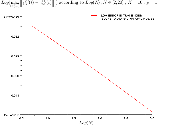
(a)

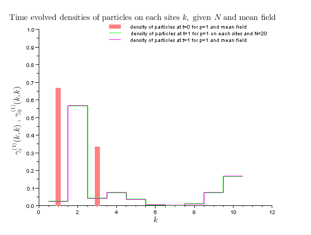
(b)

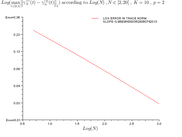
(c)

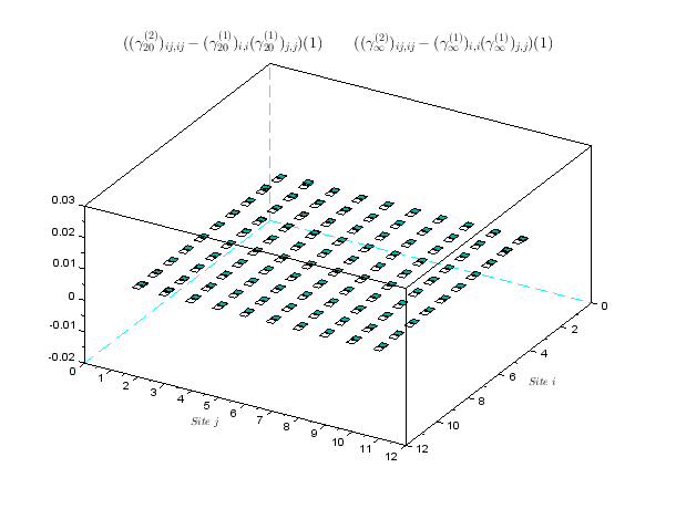
(d) Mean field(white) and 20-body quantum(blue) correlations at time $t=1$

6.2 Twin states

For the twin states $\Psi_{N}=\frac{a^{*}(\psi_{1})^{n_{1}}a^{*}(\psi_{2})^{n_{2}}}{\sqrt{\varepsilon^{n_{1}+n_{2}}n_{1}!n_{2}!}}|\Omega\rangle$, $\psi_{1}=\frac{1}{\sqrt{2}}(e_{1}+\mathrm{i}e_{3})$ and $\psi_{2}=e_{2}$.

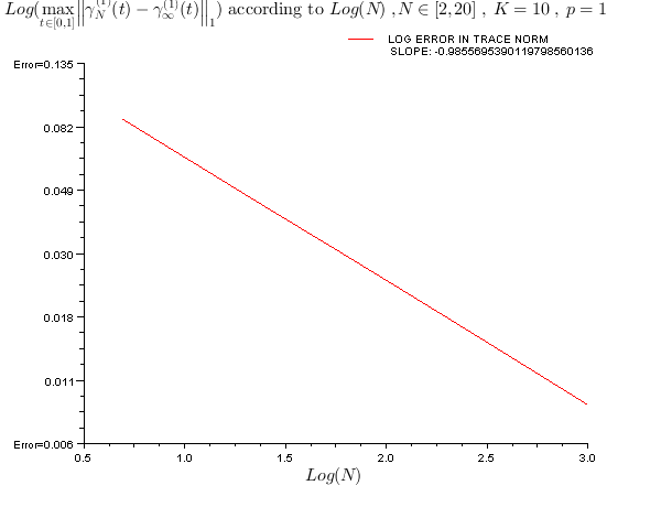
(e)

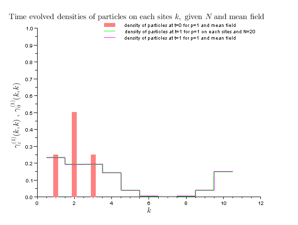
(f) Compared densities of particles at times t=0 and t=1

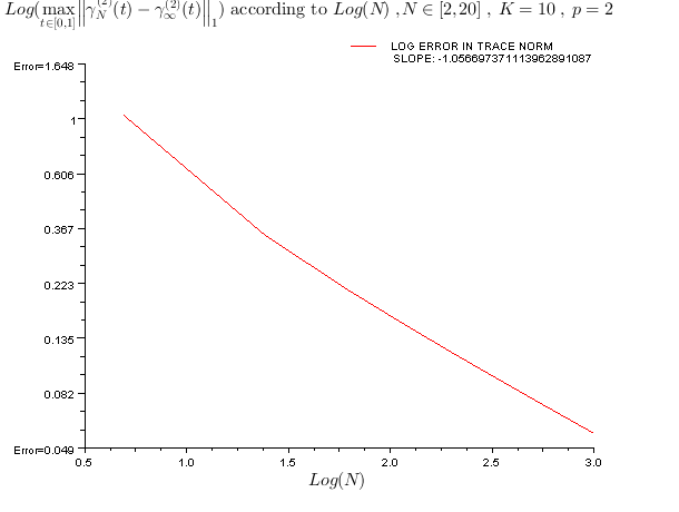
(g)

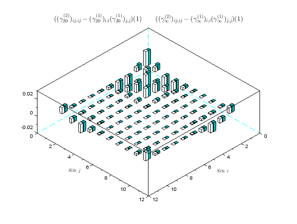
(h) Mean field(white) and 20-body quantum(blue) correlations at time $t=1$

6.3 Wq states

For the Wq states $\Psi_{N}=\frac{a^{*}(\psi_{1})^{n_{1}}a^{*}(\psi_{2})^{n_{2}}}{\sqrt{\varepsilon^{n_{1}+n_{2}}n_{1}!n_{2}!}}|\Omega\rangle$, $\psi_{1}=\frac{1}{\sqrt{2}}(e_{1}+\mathrm{i}e_{3})$ and $\psi_{2}=e_{2}$.

In this case the state is given by $S_{N}(\psi_{1}^{\otimes n_{1}}\otimes\psi_{2}^{\otimes n_{2}})$, with $n_{1}+n_{2}=N$, $n_{1}=N-q$ and $n_{2}=q$ fixed for the mean field.
The associated Wigner measure is $\delta^{S^{1}}_{\psi_{1}}$.
In these simulations $q=2$.

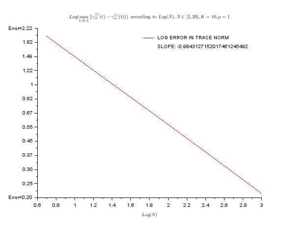
(i)

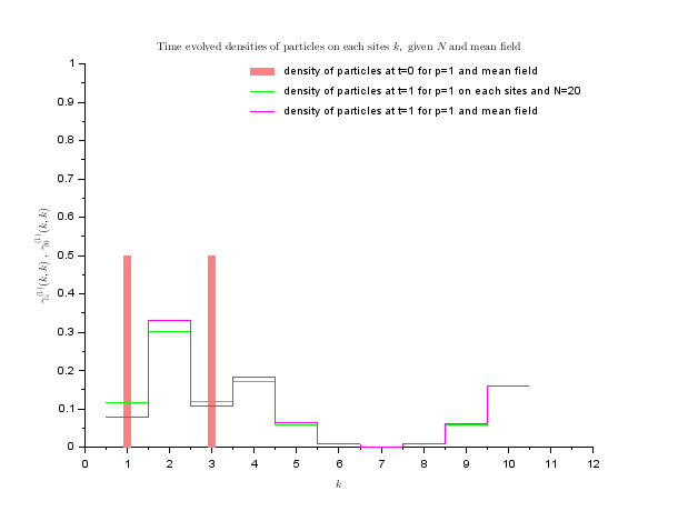
(j) Compared densities of particles at times t=0 and t=1

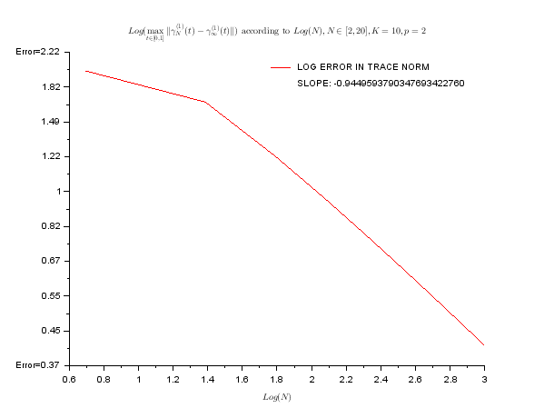
(k)

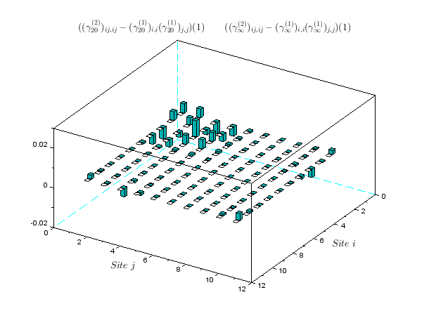
(l) Mean field(white) and 20-body quantum(blue) correlations at time $t=1$

6.4 Other states

A case when the order of convergence is equal to $1/2$.(see[1])
In this case $\varrho_{\varepsilon}=|\phi_{N}^{\otimes N}\rangle\langle\phi_{N}^{\otimes N}|$ with $\phi_{N}=\frac{1}{\sqrt{N}}e_{1}+\sqrt{1-\frac{1}{N}}e_{2}$.
The associated Wigner measure is $\delta^{S^{1}}_{e_{2}}$.

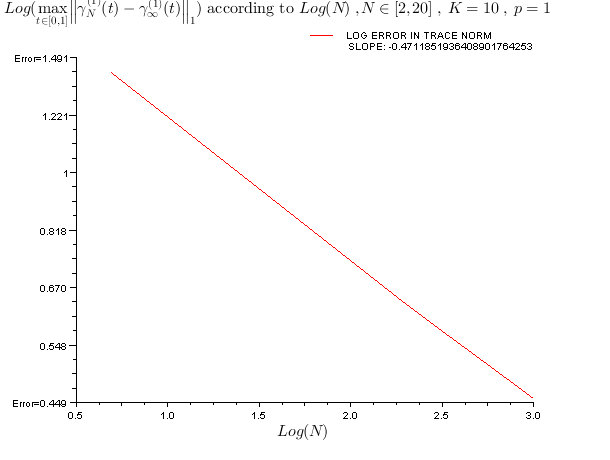
(m) Log-log plot. p=1, K=10. Numerical slope -0,4711

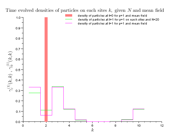
(n) Compared densities of particles at times t=0 and t=1

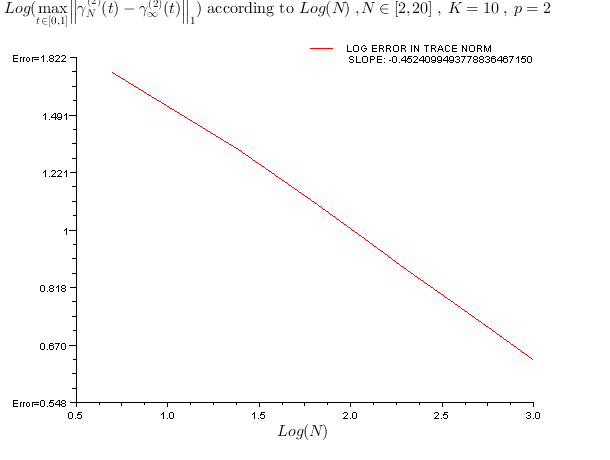
(o) Log-log plot. p=2, K=10. Numerical slope -0,4524

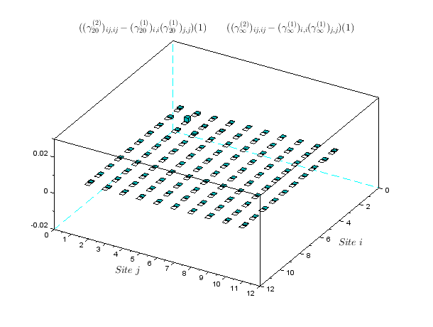
(p) Mean field(white) and 20-body quantum(blue) correlations at time $t=1$

Appendix

Class of symbols [3, 4, 5, 6]. For any $p,q\in\mathbb{N}$, define ${\mathscr{P}}_{p,q}$ to be the space of homogeneous complex-valued polynomials on ${\mathscr{Z}}$ such that $b\in{\mathscr{P}}_{p,q}$ if and only if there exists a (unique) bounded operator $\tilde{b}\in{\mathscr{L}}(\vee^{p}{\mathscr{Z}},\vee^{q}{\mathscr{Z}})$ such that for all $z\in{\mathscr{Z}}$:

$$b(z)={\langle}z^{\otimes q},\tilde{b}\,z^{\otimes p}{\rangle}\,.$$ (14)

$$b^{Wick}\,_{|\vee^{n}{\mathscr{Z}}}=1_{[p,+\infty)}(n)\frac{\sqrt{n!(n+q-p)!}}{(n-p)!}\;{\varepsilon}^{\frac{p+q}{2}}\;{\mathcal{S}}_{n-p+q}\left(\tilde{b}\otimes 1^{\otimes(n-p)}\right)\,,$$ (15)

where $\tilde{b}$ denotes the operator associated with the symbol $b$ according to (14).

The composition method based on the Strang splitting with the coefficients (12) is of $4^{th}$ order (see [35]).

Dimension of $\bigvee^{N}\mathbb{C}^{K}$: $\dbinom{N+K-1}{K-1}$ for $K$ in $[1,10]$ and $N$ in $[1,20]$:

	$K=1$	2	3	4	5	6	7	8	9	10
$N=1$	1	2	3	4	5	6	7	8	9	10
2	1	3	6	10	15	21	28	36	45	55
3	1	4	10	20	35	56	84	120	165	220
4	1	5	15	35	70	126	210	330	495	715
5	1	6	21	56	126	252	462	792	1287	2002
6	1	7	28	84	210	462	924	1716	3003	5005
7	1	8	36	120	330	792	1716	3432	6435	11440
8	1	9	45	165	495	1287	3003	6435	12870	24310
9	1	10	55	220	715	2002	5005	11440	24310	48620
10	1	11	66	286	1001	3003	8008	19448	43758	92378
11	1	12	78	364	1365	4368	12376	31824	75582	167960
12	1	13	91	455	1820	6188	18564	50388	125970	293930
13	1	14	105	560	2380	8568	27132	77520	203490	497420
14	1	15	120	680	3060	11628	38760	116280	319770	817190
15	1	16	136	816	3876	15504	54264	170544	490314	1307504
16	1	17	153	969	4845	20349	74613	245157	735471	2042975
17	1	18	171	1140	5985	26334	100947	346104	1081575	3124550
18	1	19	190	1330	7315	33649	134596	480700	1562275	4686825
19	1	20	210	1540	8855	42504	177100	657800	2220075	6906900
20	1	21	231	1771	10626	53130	230230	888030	3108105	10015005

References

- [1] Z. Ammari, M. Falconi, B. Pawilowski On the rate of convergence for the mean field approximation of many-body quantum dynamics arXiv 1411.6284
- [2] Z. Ammari and S. Breteaux. Propagation of chaos for many-boson systems in one dimension with a point pair-interaction. Asymptot. Anal., 76(3-4):123–170, 2012.
- [3] Z. Ammari, F. Nier. Mean field limit for bosons and infinite dimensional phase-space analysis. Ann. Henri Poincaré 9 (2008), 1503–1574.
- [4] Z. Ammari, F. Nier. Mean field limit for bosons and propagation of Wigner measures. J. Math. Phys. 50 (2009).
- [5] Z. Ammari, F. Nier. Mean field propagation of Wigner measures and BBGKY hierarchies for general bosonic states. J. Math. Pures Appl. 95 (2011), 585–626.
- [6] Z. Ammari and F. Nier. Mean field propagation of infinite dimensional Wigner measures with a singular two-body interaction potential. Ann. Sc. Norm. Super. Pisa Cl. Sci.(5) Vol. XIV (2015),155-220
- [7] I. Anapolitanos. Rate of Convergence Towards the Hartree von Neumann Limit in the Mean-Field Regime, Lett Math Phys 98 (2011), 1–31.
- [8] C. Bardos, N.J Mauser. The weak coupling limit for systems of quantum particles. State of the art and applications.
- [9] C. Bardos, F. Golse, N. Mauser. Weak coupling limit of the n-particle Schrödinger equation. Methods Appl. Anal. 7 (2000), 275–293.
- [10] C. Bardos, L. Erdös, F. Golse, N. Mauser, H-T. Yau. Derivation of the Schrödinger-Poisson equation from the quantum N-body problem. C.R. Math. Acad. Sci. Paris 334 (2002), 515–520.
- [11] F.A. Berezin. The method of second quantization. Second edition. “Nauka”, Moscow, (1986).
- [12] J.M. Bony, N. Lerner. Quantification asymptotique et microlocalisation d’ordre supérieur I. Ann. Scient. Ec. Norm. Sup., série 22 (1989), 377–433.
- [13] X. Chen. Second order corrections to mean field evolution for weakly interacting bosons in the case of three-body interactions. Arch. Ration. Mech. Anal. 203, (2012), no 2, 455–497.
- [14] L. Chen, J.O. Lee, B. Schlein. Rate of convergence towards Hartree dynamics. J. Stat. Phys. 144, (2011), No. 4, 872–903.
- [15] T. Chen, N. Pavlović. The quintic NLS as the mean field limit of a boson gas with three-body interactions. J. Funct. Anal. 260 (2011), no. 4, 959–997.
- [16] T. Chen, C. Hainzl, N. Pavlović, R. Seiringer. On the well-posedness and scattering for the Gross-Pitaevskii hierarchy via quantum de Finetti. Lett. Math. Phys. 104, (2014), 871–891.
- [17] G. F. Dell’Antonio. On the limits of sequences of normal states. Comm. Pure Appl. Math., 20 (1967), 413–429.
- [18] J. Dereziński, C. Gérard. Mathematics of quantization and quantum fields. Cambridge Monographs on Mathematical Physics, Cambridge University Press, (2013).
- [19] A. Elgart, B. Schlein. Mean field dynamics of boson stars Comm. Pure and Appl. Math. Vol. 60, (2005) 500–545.
- [20] L. Erdös, H.T. Yau. Derivation of the nonlinear Schrödinger equation from a many body Coulomb system. Adv. Theor. Math. Phys. 5 (2001), 1169–2005.
- [21] L. Erdös, B. Schlein, H.T. Yau. Derivation of the cubic non-linear Schrödinger equation from quantum dynamics of many-body systems. Invent. Math. 167 no. 3 (2007), 515–614.
- [22] L. Erdös, B. Schlein, H.T. Yau. Derivation of the Gross-Pitaevskii equation for the dynamics of Bose-Einstein condensate. Ann. of Math. (2) 172 (2010), no. 1, 291-370.
- [23] M. Falconi. Mean field limit of bosonic systems in partially factorized states and their linear combinations. Arxiv http://fr.arxiv.org/abs/1305.5699.
- [24] J. Fröhlich, S. Graffi, S. Schwarz. Mean-field- and classical limit of many-body Schrödinger dynamics for bosons. Comm. Math. Phys. 271, No. 3 (2007), 681–697.
- [25] J. Fröhlich, A. Knowles, A. Pizzo. Atomism and quantization. J. Phys. A 40, no. 12 (2007), 3033–3045.
- [26] J. Fröhlich, A. Knowles, S. Schwarz. On the Mean-field limit of bosons with Coulomb two-body interaction Comm. Math. Phys. 288, No. 3 (2009), 1023–1059.
- [27] P. Gérard. Microlocal defect measures. Comm. Partial Differential Equations 16 (1991), no. 11, 1761-1794.
- [28] P. Gérard, P.A. Markowich, N.J. Mauser, F. Poupaud. Homogenization limits and Wigner transforms. Comm. Pure Appl. Math. 50 no. 4 (1997), 323–379.
- [29] J. Ginibre, G. Velo. The classical field limit of scattering theory for nonrelativistic many-boson systems. I. Comm. Math. Phys. 66 (1979), 37–76.
- [30] J. Ginibre, G. Velo. The classical field limit of scattering theory for nonrelativistic many-boson systems. II. Comm. Math. Phys. 68, (1979), 45–68.
- [31] M. Grillakis, M. Machedon, D. Margetis. Second-order corrections to mean field evolution of weakly interacting bosons. I. Comm. Math. Phys. 294, (2010), no 1, 273–301.
- [32] S. Graffi, A. Martinez, M. Pulvirenti. Mean-field approximation of quantum systems and classical limit. Math. Models Methods Appl. Sci. 13 No. 1 (2003), 59–73.
- [33] K. Hepp. The classical limit for quantum mechanical correlation functions. Comm. Math. Phys. 35 (1974), 265–277.
- [34] R. L. Hudson. Analogs of de Finetti’s theorem and interpretative problems of quantum mechanics. Found. Phys., 11(9-10):805–808, 1981.
- [35] Hairer, Ernst and Lubich, Christian and Wanner, Gerhard Geometric numerical integration Springer Series in Computational Mathematics 31 Structure-preserving algorithms for ordinary differential equations,Springer-Verlag (2002)
- [36] R. L. Hudson and G. R. Moody. Locally normal symmetric states and an analogue of de Finetti’s theorem. Z. Wahrscheinlichkeitstheorie und Verw. Gebiete,33(4):343–351, 1975/76.
- [37] S. Klainerman, M. Machedon. On the uniqueness of solutions to the Gross-Pitaevskii hierarchy. Comm. Math. Phys. 279, (2008).
- [38] A. Knowles, P. Pickl. Mean-field dynamics: singular potentials and rate of convergence. Comm. Math. Phys. 298 (2010), 101–138.
- [39] C. J. Lennard. is uniformly Kadec-Klee. Proc. Amer. Math. Soc. 109 (1990), 71–77.
- [40] M. Lewin, P.T. Nam, N. Rougerie. Remarks on the quantum de Finetti theorem for bosonic systems. Appl. Math. Res. Express (AMRX), in press, 2014.
- [41] M. Lewin, P.T. Nam, N. Rougerie. Derivation of Hartree’s theory for generic mean-field Bose gases. Adv. Math., 254, (2014), 570–621.
- [42] Q. Liard, B. Pawilowski. Mean field limit for bosons with compact kernels interactions by Wigner measures transportation. J. Math. Phys. 55, 092304 (2014).
- [43] E.H. Lieb, R. Seiringer, J.P. Solovej, J. Yngvason. The mathematics of the Bose gas and its condensation. Birkhäuser (2005).
- [44] P.L. Lions, T. Paul. Sur les mesures de Wigner. Rev. Mat. Iberoamericana 9 no. 3 (1993), 553–618.
- [45] A. Martinez. An Introduction to Semiclassical Analysis and Microlocal Analysis. Universitext, Springer-Verlag, (2002).
- [46] P. Pickl. A simple derivation of mean field limits for quantum systems. Lett. Math. Phys. 97 (2011) 151–164.
- [47] B. Simon. Trace ideals and their applications. Second edition. Mathematical Surveys and Monographs, 120. AMS, Providence, RI, 2005.
- [48] D. Robert. Autour de l’approximation semi-classique. Progress in Mathematics, 68. Birkhäuser (1987).
- [49] I. Rodnianski, B. Schlein. Quantum Fluctuations and Rate of Convergence towards Mean Field Dynamics. Comm. Math. Phys. 291, No 1 (2009), 31–61.
- [50] H. Spohn. Kinetic equations from Hamiltonian dynamics. Rev. Mod. Phys. 52, No. 3 (1980), 569–615.