$f$-Divergence Inequalities

Abstract

This paper develops systematic approaches to obtain $f$-divergence inequalities, dealing with pairs of probability measures defined on arbitrary alphabets. Functional domination is one such approach, where special emphasis is placed on finding the best possible constant upper bounding a ratio of $f$-divergences. Another approach used for the derivation of bounds among $f$-divergences relies on moment inequalities and the logarithmic-convexity property, which results in tight bounds on the relative entropy and Bhattacharyya distance in terms of $\chi^{2}$ divergences. A rich variety of bounds are shown to hold under boundedness assumptions on the relative information. Special attention is devoted to the total variation distance and its relation to the relative information and relative entropy, including “reverse Pinsker inequalities,” as well as on the $E_{\gamma}$ divergence, which generalizes the total variation distance. Pinsker’s inequality is extended for this type of $f$-divergence, a result which leads to an inequality linking the relative entropy and relative information spectrum. Integral expressions of the Rényi divergence in terms of the relative information spectrum are derived, leading to bounds on the Rényi divergence in terms of either the variational distance or relative entropy.

Keywords: relative entropy, total variation distance, $f$-divergence, Rényi divergence, Pinsker’s inequality, relative information.

I Introduction

Throughout their development, information theory, and more generally, probability theory, have benefitted from non-negative measures of dissimilarity, or loosely speaking, distances, between pairs of probability measures defined on the same measurable space (see, e.g., [41, 65, 105]). Notable among those measures are (see Section II for definitions):

• total variation distance $|P-Q|$;

• relative entropy $D(P\|Q)$;

• $\chi^{2}$-divergence $\chi^{2}(P\|Q)$;

• Hellinger divergence $\mathscr{H}_{\alpha}(P\|Q)$;

• Rényi divergence $D_{\alpha}(P\|Q)$.

It is useful, particularly in proving convergence results, to give bounds of one measure of dissimilarity in terms of another. The most celebrated among those bounds is Pinsker’s inequality:

$$\tfrac{1}{2}|P-Q|^{2}\log e\leq D(P\|Q)$$ (1)

proved by Csiszár [23] and Kullback [60], with Kemperman [56] independently a bit later. Improved and generalized versions of Pinsker’s inequality have been studied, among others, in [39], [44], [46], [76], [86], [92], [103].

Relationships among measures of distances between probability measures have long been a focus of interest in probability theory and statistics (e.g., for studying the rate of convergence of measures). The reader is referred to surveys in [41, Section 3], [65, Chapter 2], [86] and [87, Appendix 3], which provide several relationships among useful $f$-divergences and other measures of dissimilarity between probability measures. Some notable existing bounds among $f$-divergences include, in addition to (1):

• [63, Lemma 1], [64, p. 25]

  $$\mathscr{H}_{\frac{1}{2}}^{2}(P\|Q) \leq|P-Q|^{2}$$ (2)

  $$\leq\mathscr{H}_{\frac{1}{2}}(P\|Q)\,\bigl{(}4-\mathscr{H}_{\frac{1}{2}}(P\|Q)\bigr{)};$$ (3)

• [15, (2.2)]

  $$\tfrac{1}{4}|P-Q|^{2}\leq 1-\exp\bigl{(}-D(P\|Q)\bigr{)};$$ (4)

• [41, Theorem 5], [35, Theorem 4], [99]

  $$D(P\|Q) \leq\log\bigl{(}1+\chi^{2}(P\|Q)\bigr{)};$$ (5)

• [48, Corollary 5.6] For all $\alpha\geq 2$

  $$\chi^{2}(P\|Q)\leq\Bigl{(}1+(\alpha-1)\,\mathscr{H}_{\alpha}(P\|Q)\Bigr{)}^{\frac{1}{\alpha-1}}-1;$$ (6)

  the inequality in (6) is reversed if $\alpha\in(0,1)\cup(1,2]$, and it holds with equality if $\alpha=2$.

• [44, 45], [86, (58)]

  $$\chi^{2}(P\|Q)\geq\left\{\begin{array}[]{ll}|P-Q|^{2},&\quad\mbox{$|P-Q|\in\bigl{[}0,1]$}\\[5.69046pt] \frac{|P-Q|}{2-|P-Q|},&\quad\mbox{$|P-Q|\in\bigl{(}1,2)$.}\end{array}\right.$$ (9)

• [96]

  $$\frac{D^{2}(P\|Q)}{D(Q\|P)} \leq\tfrac{1}{2}\,\chi^{2}(P\|Q)\,\log e;$$ (10)

  $$4\,\mathscr{H}^{2}_{\frac{1}{2}}(P\|Q)\,\log^{2}e \leq D(P\|Q)\;D(Q\|P)$$ (11)

  $$\leq\tfrac{1}{4}\,\chi^{2}(P\|Q)\;\chi^{2}(Q\|P)\,\log^{2}e;$$ (12)

  $$4\,\mathscr{H}_{\frac{1}{2}}(P\|Q)\,\log e \leq D(P\|Q)+D(Q\|P)$$ (13)

  $$\leq\tfrac{1}{2}\,\bigl{(}\chi^{2}(P\|Q)+\chi^{2}(Q\|P)\bigr{)}\,\log e;$$ (14)

• [32, (2.8)]

  $$D(P\|Q)\leq\tfrac{1}{2}\left(|P-Q|+\chi^{2}(P\|Q)\right)\log e\,;$$ (15)

• [46], [86, Corollary 32], [91]

  $$D(P\|Q)+D(Q\|P)\geq|P-Q|\;\log\left(\frac{2+|P-Q|}{2-|P-Q|}\right),$$ (16)

  $$\chi^{2}(P\|Q)+\chi^{2}(Q\|P)\geq\frac{8\,|P-Q|^{2}}{4-|P-Q|^{2}};$$ (17)

• [53, p. 711] (cf. a generalized form in [87, Lemma A.3.5])

  $$\mathscr{H}_{\frac{1}{2}}(P\|Q)\,\log e\leq D(P\|Q),$$ (18)

  generalized in [65, Proposition 2.15]:

  $$\mathscr{H}_{\alpha}(P\|Q)\,\log e\leq D_{\alpha}(P\|Q)\leq D(P\|Q),$$ (19)

  for $\alpha\in(0,1)$, and

  $$\mathscr{H}_{\alpha}(P\|Q)\,\log e\geq D_{\alpha}(P\|Q)\geq D(P\|Q)$$ (20)

  for $\alpha\in(1,\infty)$.

• [65, Proposition 2.35] If $\alpha\in(0,1)$, $\beta\triangleq\max\{\alpha,1-\alpha\}$, then

  $$1-\left(1+\tfrac{1}{2}\,|P-Q|\right)^{\beta}\left(1-\tfrac{1}{2}\,|P-Q|\right)^{1-\beta}$$

  $$\leq(1-\alpha)\,\mathscr{H}_{\alpha}(P\|Q)$$ (21)

  $$\leq\tfrac{1}{2}\,|P-Q|.$$ (22)

• [37, Theorems 3 and 16]

  • $D_{\alpha}(P\|Q)$ is monotonically increasing in $\alpha>0$;

  • $\left(\frac{1}{\alpha}-1\right)D_{\alpha}(P\|Q)$ is monotonically decreasing in $\alpha\in(0,1]$;

  • [65, Proposition 2.7] the same monotonicity properties hold for $\mathscr{H}_{\alpha}(P\|Q)$.

• [46] If $\alpha\in(0,1]$, then

  $$\frac{\alpha}{2}\,|P-Q|^{2}\log e\leq D_{\alpha}(P\|Q);$$ (23)

• An inequality for $\mathscr{H}_{\alpha}(P\|Q)$ [61, Lemma 1] becomes (at $\alpha=1$), the parallelogram identity [26, (2.2)]

  $$D(P_{0}\|Q)+D(P_{1}\|Q)=D(P_{0}\|P_{\frac{1}{2}})+D(P_{1}\|P_{\frac{1}{2}})+2D(P_{\frac{1}{2}}\|Q).$$ (24)

  with $P_{\frac{1}{2}}=\tfrac{1}{2}(P_{0}+P_{1})$, and extends a result for the relative entropy in [26, Theorem 2.1].

• A “reverse Pinsker inequality”, providing an upper bound on the relative entropy in terms of the total variation distance, does not exist in general since we can find distributions which are arbitrarily close in total variation but with arbitrarily high relative entropy. Nevertheless, it is possible to introduce constraints under which such reverse Pinsker inequalities hold. In the special case of a finite alphabet $\mathcal{A}$, Csiszár and Talata [29, p. 1012] showed that

  $$D(P\|Q)\leq\left(\frac{\log e}{Q_{\min}}\right)\cdot|P-Q|^{2}$$ (25)

  when $Q_{\min}\triangleq\min_{a\in\mathcal{A}}Q(a)$ is positive.

• [25, Theorem 3.1] if $f\colon(0,\infty)\to\mathbb{R}$ is a strictly convex function, then there exists a real-valued function $\psi_{f}$ such that $\lim_{x\downarrow 0}\psi_{f}(x)=0$ and

  $$|P-Q|\leq\psi_{f}\bigl{(}D_{f}(P\|Q)\bigr{)}.$$ (26)

  which implies

  $$\lim_{n\to\infty}D_{f}(P_{n}\|Q_{n})=0\;\Rightarrow\;\lim_{n\to\infty}|P_{n}-Q_{n}|=0.$$ (27)

The numerical optimization of an $f$-divergence subject to simultaneous constraints on $f_{i}$-divergences $(i=1,\ldots,L)$ was recently studied in [48], which showed that for that purpose it is enough to restrict attention to alphabets of cardinality $L+2$. Earlier, [50] showed that if $L=1$, then either the solution is obtained by a pair $(P,Q)$ on a binary alphabet, or it is a deflated version of such a point. Therefore, from a purely numerical standpoint, the minimization of $D_{f}(P\|Q)$ such that $D_{g}(P\|Q)\geq d$ can be accomplished by a grid search on $[0,1]^{2}$. Occasionally, as in the case where $D_{f}(P\|Q)=D(P\|Q)$ and $D_{g}(P\|Q)=|P-Q|$, it is actually possible to determine analytically the locus of $(D_{f}(P\|Q),D_{g}(P\|Q))$ (see [39]). In fact, as shown in [104, (22)], a binary alphabet suffices if the single constraint is on the total variation distance. The same conclusion holds when minimizing the Rényi divergence [92].

In this work, we find relationships among the various divergence measures outlined above as well as a number of other measures of dissimilarity between probability measures. The framework of $f$-divergences, which encompasses the foregoing measures (Rényi divergence is a one-to-one transformation of the Hellinger divergence) serves as a convenient playground.

The rest of the paper is structured as follows:

Section II introduces the basic definitions needed and in particular the various measures of dissimilarity between probability measures used throughout.

Based on functional domination, Section III provides a basic tool for the derivation of bounds among $f$-divergences. Under mild regularity conditions, this approach further enables to prove the optimality of constants in those bounds. In addition, we show instances where such optimality can be shown in the absence of regularity conditions. The basic tool used in Section III is exemplified in obtaining relationships among important $f$-divergences such as relative entropy, Hellinger divergence and total variation distance. This approach is also useful in strengthening and providing an alternative proof of Samson’s inequality [89] (a counterpart to Pinsker’s inequality using Marton’s divergence, useful in proving certain concentration of measure results [13]), whose constant we show cannot be improved. In addition, we show several new results in Section III-E on the maximal ratios of various $f$-divergences to total variation distance.

Section IV provides an approach for bounding ratios of $f$-divergences, assuming that the relative information (see Definition 1) is lower and/or upper bounded with probability one. The approach is exemplified in bounding ratios of relative entropy to various $f$-divergences, and analyzing the local behavior of $f$-divergence ratios when the reference measure is fixed. We also show that bounded relative information leads to a strengthened version of Jensen’s inequality, which, in turn, results in upper and lower bounds on the ratio of the non-negative difference $\log\left(1+\chi^{2}(P\|Q)\right)-D(P\|Q)$ to $D(Q\|P)$. A new reverse version of Samson’s inequality is another byproduct of the main tool in this section.

The rich structure of the total variation distance as well as its importance in both fundamentals and applications merits placing special attention on bounding the rest of the distance measures in terms of $|P-Q|$. Section V gives several useful identities linking the total variation distance with the relative information spectrum, which result in a number of upper and lower bounds on $|P-Q|$, some of which are tighter than Pinsker’s inequality in various ranges of the parameters. It also provides refined bounds on $D(P\|Q)$ as a function of $\chi^{2}$-divergences and the total variation distance.

Section VI is devoted to proving “reverse Pinsker inequalities,” namely, lower bounds on $|P-Q|$ as a function of $D(P\|Q)$ involving either (a) bounds on the relative information, (b) Lipschitz constants, or (c) the minimum mass of the reference measure (in the finite alphabet case). In the latter case, we also examine the relationship between entropy and the total variation distance from the equiprobable distribution, as well as the exponential decay of the probability that an independent identically distributed sequence is not strongly typical.

Section VII focuses on the $E_{\gamma}$ divergence. This $f$-divergence generalizes the total variation distance, and its utility in information theory has been exemplified in [18, 68, 69, 70, 79, 80, 81]. Based on the operational interpretation of the DeGroot statistical information [31] and the integral representation of $f$-divergences as a function of DeGroot’s measure, Section VII provides an integral representation of $f$-divergences as a function of the $E_{\gamma}$ divergence; this representation shows that $\{(E_{\gamma}(P\|Q),E_{\gamma}(Q\|P)),\gamma\geq 1\}$ uniquely determines $D(P\|Q)$ and $\mathscr{H}_{\alpha}(P\|Q)$, as well as any other $f$-divergence with twice differentiable $f$. Accordingly, bounds on the $E_{\gamma}$ divergence directly translate into bounds on other important $f$-divergences. In addition, we show an extension of Pinsker’s inequality (1) to $E_{\gamma}$ divergence, which leads to a relationship between the relative information spectrum and relative entropy.

The Rényi divergence, which has found a plethora of information-theoretic applications, is the focus of Section VIII. Expressions of the Rényi divergence are derived in Section VIII-A as a function of the relative information spectrum. These expressions lead in Section VIII-B to the derivation of bounds on the Rényi divergence as a function of the variational distance under the boundedness assumption of the relative information. Bounds on the Rényi divergence of an arbitrary order are derived in Section VIII-C as a function of the relative entropy when the relative information is bounded.

II Basic Definitions

II-A Relative Information and Relative Entropy

We assume throughout that the probability measures $P$ and $Q$ are defined on a common measurable space $(\mathcal{A},\mathscr{F})$, and $P\ll Q$ denotes that $P$ is absolutely continuous with respect to $Q$, namely there is no event $\mathcal{F}\in\mathscr{F}$ such that $P(\mathcal{F})>0=Q(\mathcal{F})$.

Definition 1

If $P\ll Q$, the relative information provided by $a\in\mathcal{A}$ according to $(P,Q)$ is given by

$$\imath_{P\|Q}(a)\triangleq\log\frac{\text{d}P}{\text{d}Q}\,(a).$$ (28)

When the argument of the relative information is distributed according to $P$, the resulting real-valued random variable is of particular interest. Its cumulative distribution function and expected value are known as follows.

Definition 2

If $P\ll Q$, the relative information spectrum is the cumulative distribution function

$$\mathds{F}_{P\|Q}(x)=\mathbb{P}\bigl{[}\imath_{P\|Q}(X)\leq x\bigr{]},$$ (29)

with $X\sim P$. The relative entropy of $P$ with respect to $Q$ is

$$D(P\|Q) =\mathbb{E}\bigl{[}\imath_{P\|Q}(X)\bigr{]}$$ (30)

$$=\mathbb{E}\bigl{[}\imath_{P\|Q}(Y)\,\exp\bigl{(}\imath_{P\|Q}(Y)\bigr{)}\bigr{]},$$ (31)

where $Y\sim Q$.

II-B $f$-Divergences

Introduced by Ali-Silvey [2] and Csiszár [21, 23], a useful generalization of the relative entropy, which retains some of its major properties (and, in particular, the data processing inequality [112]), is the class of $f$-divergences. A general definition of an $f$-divergence is given in [66, p. 4398], specialized next to the case where $P\ll Q$.

Definition 3

Let $f\colon(0,\infty)\to\mathbb{R}$ be a convex function, and suppose that $P\ll Q$. The $f$-divergence from $P$ to $Q$ is given by

$$D_{f}(P\|Q) =\int f\left(\frac{\text{d}P}{\text{d}Q}\right)\,\text{d}Q$$ (32)

$$=\mathbb{E}\bigl{[}f(Z)\bigr{]}$$ (33)

where

$$Z=\exp\bigl{(}\imath_{P\|Q}(Y)\bigr{)},\quad Y\sim Q.$$ (34)

and in (32), we took the continuous extension

$$f(0)=\lim_{t\downarrow 0}f(t)\in(-\infty,+\infty].$$ (35)

We can also define $D_{f}(P\|Q)$ without requiring $P\ll Q$. Let $f\colon(0,\infty)\to\mathbb{R}$ be a convex function with $f(1)=0$, and let $f^{\star}\colon(0,\infty)\to\mathbb{R}$ be given by

$$f^{\star}(t)=t\,f\left(\tfrac{1}{t}\right)$$ (36)

for all $t>0$. Note that $f^{\star}$ is also convex (see, e.g., [14, Section 3.2.6]), $f^{\star}(1)=0$, and $D_{f}(P\|Q)=D_{f^{\star}}(Q\|P)$ if $P\ll\gg Q$. By definition, we take

$$f^{\star}(0)=\lim_{t\downarrow 0}f^{\star}(t)=\lim_{u\to\infty}\frac{f(u)}{u}.$$ (37)

If $p$ and $q$ denote, respectively, the densities of $P$ and $Q$ with respect to a $\sigma$-finite measure $\mu$ (i.e., $p=\frac{\text{d}P}{\text{d}\mu}$, $q=\frac{\text{d}Q}{\text{d}\mu}$), then we can write (32) as

$$D_{f}(P\|Q) =\int q\;f\left(\frac{p}{q}\right)\,\text{d}\mu$$ (38)

$$=\int_{\{pq>0\}}q\,f\left(\frac{p}{q}\right)\,\mathrm{d}\mu+f(0)\,Q(p=0)+f^{\star}(0)P(q=0).$$ (39)

Remark 1

Different functions may lead to the same $f$-divergence for all $(P,Q)$: if for an arbitrary $b\in\mathbb{R}$, we have

$$f_{b}(t)=f_{0}(t)+b\,(t-1),\quad t\geq 0$$ (40)

then

$$D_{f_{0}}(P\|Q)=D_{f_{b}}(P\|Q).$$ (41)

The following key property of $f$-divergences follows from Jensen’s inequality.

Proposition 1

If $f\colon(0,\infty)\to\mathbb{R}$ is convex and $f(1)=0$, $P\ll Q$, then

$$D_{f}(P\|Q)\geq 0.$$ (42)

If, furthermore, $f$ is strictly convex at $t=1$, then equality in (42) holds if and only if $P=Q$.

Surveys on general properties of $f$-divergences can be found in [65, 105, 106].

The assumptions of Proposition 1 are satisfied by many interesting measures of dissimilarity between probability measures. In particular, the following examples receive particular attention in this paper. As per Definition 3, in each case the function $f$ is defined on $(0,\infty)$.

1. Relative entropy [59]: $f(t)=t\,\log t$,

   $$D(P\|Q) =D_{f}(P\|Q)$$ (43)

   $$=D_{r}(P\|Q)$$ (44)

   with $r\colon(0,\infty)\to[0,\infty)$ defined as

   $$r(t)\triangleq t\log t+(1-t)\,\log e.$$ (45)

2. Relative entropy: ($P\ll\gg Q$) $f(t)=-\log t$,

   $$D(Q\|P) =D_{f}(P\|Q);$$ (46)

3. Jeffrey’s divergence [54]: ($P\ll\gg Q$) $f(t)=(t-1)\,\log t$,

   $$D(P\|Q)+D(Q\|P) =D_{f}(P\|Q);$$ (47)

4. $\chi^{2}$-divergence [77]: $f(t)=(t-1)^{2}$ or $f(t)=t^{2}-1$,

   $$\chi^{2}(P\|Q) =D_{f}(P\|Q)$$ (48)

   $$\chi^{2}(P\|Q) =\int\left(\frac{\text{d}P}{\text{d}Q}-1\right)^{2}\,\text{d}Q$$ (49)

   $$=\int\left(\frac{\text{d}P}{\text{d}Q}\right)^{2}\,\text{d}Q-1$$ (50)

   $$=\mathbb{E}\bigl{[}\exp\bigl{(}2\imath_{P\|Q}(Y)\bigr{)}\bigr{]}-1$$ (51)

   $$=\mathbb{E}\bigl{[}\exp\bigl{(}\imath_{P\|Q}(X)\bigr{)}\bigr{]}-1$$ (52)

   with $X\sim P$ and $Y\sim Q$. Note that if $P\ll\gg Q$, then from the right side of (50), we obtain

   $$\chi^{2}(Q\|P)=D_{g}(P\|Q)$$ (53)

   with $g(t)=\frac{1}{t}-t=f^{\star}(t)$, and $f(t)=t^{2}-1$.

5. Hellinger divergence of order $\alpha\in(0,1)\cup(1,\infty)$ [54], [65, Definition 2.10]:

   $$\mathscr{H}_{\alpha}(P\|Q)=D_{f_{\alpha}}(P\|Q)$$ (54)

   with

   $$f_{\alpha}(t)=\frac{t^{\alpha}-1}{\alpha-1}.$$ (55)

   The $\chi^{2}$-divergence is the Hellinger divergence of order 2, while $\tfrac{1}{2}\mathscr{H}_{\frac{1}{2}}(P\|Q)$ is usually referred to as the squared Hellinger distance. The analytic extension of $\mathscr{H}_{\alpha}(P\|Q)$ at $\alpha=1$ yields

   $$\mathscr{H}_{1}(P\|Q)\,\log e=D(P\|Q).$$ (56)

6. Total variation distance: Setting

   $$f(t)=|t-1|$$ (57)

   results in

   $$|P-Q| =D_{f}(P\|Q)$$ (58)

   $$=\int\left|\frac{\text{d}P}{\text{d}Q}-1\right|\,\text{d}Q$$ (59)

   $$=2\,\sup_{\mathcal{F}\in\mathscr{F}}\bigl{(}P(\mathcal{F})-Q(\mathcal{F})\bigr{)}.$$ (60)

7. Triangular Discrimination [62, 108] (a.k.a. Vincze-Le Cam distance):

   $$\Delta(P\|Q)=D_{f}(P\|Q)$$ (61)

   with

   $$f(t)=\frac{(t-1)^{2}}{t+1}.$$ (62)

   Note that

   $$\tfrac{1}{2}\,\Delta(P\|Q) =\chi^{2}(P\,\|\,\tfrac{1}{2}P+\tfrac{1}{2}Q)$$ (63)

   $$=\chi^{2}(Q\,\|\,\tfrac{1}{2}P+\tfrac{1}{2}Q).$$ (64)

8. Jensen-Shannon divergence [67] (a.k.a. capacitory discrimination):

   $$\mathrm{JS}(P\|Q) =D\left(P\,\|\,\tfrac{1}{2}P+\tfrac{1}{2}Q\right)+D\left(Q\,\|\,\tfrac{1}{2}P+\tfrac{1}{2}Q\right)$$ (65)

   $$=D_{f}(P\|Q)$$ (66)

   with

   $$f(t)=t\log t-(1+t)\log\left(\frac{1+t}{2}\right).$$ (67)

9. $E_{\gamma}$ divergence (see, e.g., [79, p. 2314]): For $\gamma\geq 1$,

   $$E_{\gamma}(P\|Q)=D_{f_{\gamma}}(P\|Q)$$ (68)

   with

   $$f_{\gamma}(t)=(t-\gamma)^{+}$$ (69)

   where $(x)^{+}\triangleq\max\{x,0\}$. $E_{\gamma}$ is sometimes called “hockey-stick divergence” because of the shape of $f_{\gamma}$. If $\gamma=1$, then

   $$E_{1}(P\|Q)=\tfrac{1}{2}\,|P-Q|.$$ (70)

10. DeGroot statistical information [31]: For $p\in(0,1)$,

    $$\mathcal{I}_{p}(P\|Q)=D_{\phi_{p}}(P\|Q)$$ (71)

    with

    $$\phi_{p}(t)=\min\{p,1-p\}-\min\{p,1-pt\}.$$ (72)

    Invoking (68)–(72), we get (cf. [66, (77)])

    $$\mathcal{I}_{\frac{1}{2}}(P\|Q)=\tfrac{1}{2}E_{1}(P\|Q)=\tfrac{1}{4}\,|P-Q|.$$ (73)

    This measure was first proposed by DeGroot [31] due to its operational meaning in Bayesian statistical hypothesis testing (see Section VII-B), and it was later identified as an $f$-divergence (see [66, Theorem 10]).

11. Marton’s divergence [73, pp. 558–559]:

    $$d_{2}^{2}(P,Q) =\min\mathbb{E}\left[\mathbb{P}^{2}[X\neq Y\,|\,Y]\right]$$ (74)

    $$=D_{s}(P\|Q)$$ (75)

    where the minimum is over all probability measures $P_{XY}$ with respective marginals $P_{X}=P$ and $P_{Y}=Q$, and

    $$s(t)=(t-1)^{2}\;1\{t<1\}.$$ (76)

    Note that Marton’s divergence satisfies the triangle inequality [73, Lemma 3.1], and $d_{2}(P,Q)=0$ implies $P=Q$; however, due to its asymmetry, it is not a distance measure.

II-C Rényi Divergence

Another generalization of relative entropy was introduced by Rényi [88] in the special case of finite alphabets. The general definition (assuming $P\ll Q$) is the following.

Definition 4

Let $P\ll Q$. The Rényi divergence of order $\alpha\geq 0$ from $P$ to $Q$ is given as follows:

• If $\alpha\in(0,1)\cup(1,\infty)$, then

  $$D_{\alpha}(P\|Q) =\frac{1}{\alpha-1}\;\log\Bigl{(}\mathbb{E}\bigl{[}\exp\bigl{(}\alpha\,\imath_{P\|Q}(Y)\bigr{)}\bigr{]}\Bigr{)}$$ (77)

  $$=\frac{1}{\alpha-1}\;\log\Bigl{(}\mathbb{E}\bigl{[}\exp\bigl{(}(\alpha-1)\,\imath_{P\|Q}(X)\bigr{)}\bigr{]}\Bigr{)}$$ (78)

  with $X\sim P$ and $Y\sim Q$.

• If $\alpha=0$, then

  $$D_{0}(P\|Q)=\max_{\mathcal{F}\in\mathscr{F}\colon P(\mathcal{F})=1}\log\left(\frac{1}{Q(\mathcal{F})}\right).$$ (79)

• If $\alpha=1$, then

  $$D_{1}(P\|Q)=D(P\|Q)$$ (80)

  which is the analytic extension of $D_{\alpha}(P\|Q)$ at $\alpha=1$. If $D(P\|Q)<\infty$, it can be verified by L’Hôpital’s rule that $D(P\|Q)=\lim_{\alpha\uparrow 1}D_{\alpha}(P\|Q)$.

• If $\alpha=+\infty$ then

  $$D_{\infty}(P\|Q)=\log\left(\operatorname*{ess\,sup}\frac{\text{d}P}{\text{d}Q}\,(Y)\right)$$ (81)

  with $Y\sim Q$. If $P\not\ll Q$, we take $D_{\infty}(P\|Q)=\infty$.

Rényi divergence is a one-to-one transformation of Hellinger divergence of the same order $\alpha\in(0,1)\cup(1,\infty)$:

$$D_{\alpha}(P\|Q)=\frac{1}{\alpha-1}\;\log\left(1+(\alpha-1)\,\mathscr{H}_{\alpha}(P\|Q)\right)$$ (82)

which, when particularized to order 2 becomes

$$D_{2}(P\|Q)=\log\left(1+\chi^{2}(P\|Q)\right).$$ (83)

Note that (6), (19), (20) follow from (82) and the monotonicity of the Rényi divergence in its order, which in turn yields (18).

Introduced in [8], the Bhattacharyya distance was popularized in the engineering literature in [55].

Definition 5

The Bhattacharyya distance between $P$ and $Q$, denoted by $B(P\|Q)$, is given by

$$B(P\|Q) =\tfrac{1}{2}\,D_{\frac{1}{2}}(P\|Q)$$ (84)

$$=\log\biggl{(}\frac{1}{1-\tfrac{1}{2}\mathscr{H}_{\frac{1}{2}}(P\|Q)}\biggr{)}.$$ (85)

Note that, if $P\ll\gg Q$, then $B(P\|Q)=B(Q\|P)$ and $B(P\|Q)=0$ if and only if $P=Q$, though $B(P\|Q)$ does not satisfy the triangle inequality.

III Functional Domination

Let $f$ and $g$ be convex functions on $(0,\infty)$ with $f(1)=g(1)=0$, and let $P$ and $Q$ be probability measures defined on a measurable space $(\mathcal{A},\mathscr{F})$. If there exists $\alpha>0$ such that $f(t)\leq\alpha g(t)$ for all $t\in(0,\infty)$, then it follows from Definition 3 that

$$D_{f}(P\|Q)\leq\alpha\,D_{g}(P\|Q).$$ (86)

This simple observation leads to a proof of, for example, (18) and the left inequality in (2) with the aid of Remark 1.

III-A Basic Tool

Theorem 1

Let $P\ll Q$, and assume

• $f$ is convex on $(0,\infty)$ with $f(1)=0$;

• $g$ is convex on $(0,\infty)$ with $g(1)=0$;

• $g(t)>0$ for all $t\in(0,1)\cup(1,\infty)$.

Denote the function $\kappa\colon(0,1)\cup(1,\infty)\to\mathbb{R}$

$$\kappa(t) =\frac{f(t)}{g(t)},\quad t\in(0,1)\cup(1,\infty)$$ (87)

and

$$\bar{\kappa} =\sup_{t\in(0,1)\cup(1,\infty)}\kappa(t).$$ (88)

Then,

1. $$D_{f}(P\|Q)\leq\bar{\kappa}\,D_{g}(P\|Q).$$ (89)

2. If, in addition, $f^{\prime}(1)=g^{\prime}(1)=0$, then

   $$\sup_{P\neq Q}\frac{D_{f}(P\|Q)}{D_{g}(P\|Q)}=\bar{\kappa}.$$ (90)

Proof:

1. The bound in (89) follows from (86) and $f(t)\leq\bar{\kappa}\,g(t)$ for all $t>0$.

2. Since $g$ is positive except at $t=1$, $D_{g}(P\|Q)>0$ if $P\neq Q$. The convexity of $f,g$ on $(0,\infty)$ implies their continuity; and since $g(t)>0$ for all $t\in(0,1)\cup(1,\infty)$, $\kappa(\cdot)$ is continuous on both $(0,1)$ and $(1,\infty)$.

   To show (90), we fix an arbitrary $\nu\in(0,1)\cup(1,\infty)$ and construct a sequence of pairs of probability measures whose ratio of $f$-divergence to $g$-divergence converges to $\kappa(\nu)$. To that end, for sufficiently small $\varepsilon>0$, let $P_{\varepsilon}$ and $Q_{\varepsilon}$ be parametric probability measures defined on the set $\mathcal{A}=\{0,1\}$ with $P_{\varepsilon}(0)=\nu\,\varepsilon$ and $Q_{\varepsilon}(0)=\varepsilon$. Then,

   $$\lim_{\varepsilon\to 0}\,\frac{D_{f}(P_{\varepsilon}\|Q_{\varepsilon})}{D_{g}(P_{\varepsilon}\|Q_{\varepsilon})} =\lim_{\varepsilon\to 0}\,\frac{\varepsilon\,f(\nu)+(1-\varepsilon)\,f\left(\frac{1-\nu\varepsilon}{1-\varepsilon}\right)}{\varepsilon\,g(\nu)+(1-\varepsilon)\,g\left(\frac{1-\nu\varepsilon}{1-\varepsilon}\right)}$$ (91)

   $$=\lim_{\alpha\to 0}\frac{f(\nu)+\frac{\nu-1}{\alpha}\;f(1-\alpha)}{g(\nu)+\frac{\nu-1}{\alpha}\;g(1-\alpha)}$$ (92)

   $$=\kappa(\nu)$$ (93)

   where (92) holds by change of variable $\varepsilon=\alpha/(\nu-1+\alpha)$, and (93) holds by the assumption on the derivatives of $f$ and $g$ at 1, the assumption that $f(1)=g(1)=0$, and the continuity of $\kappa(\cdot)$ at $\nu$. If $\bar{\kappa}=\kappa(\nu)$ we are done. If the supremum in (88) is not attained on $(0,1)\cup(1,\infty)$, then the right side of (93) can be made arbitrarily close to $\bar{\kappa}$ by an appropriate choice of $\nu$.

∎

Remark 2

Beyond the restrictions in Theorem 1a), the only operative restriction imposed by Theorem 1b) is the differentiability of the functions $f$ and $g$ at $t=1$. Indeed, we can invoke Remark 1 and add $f^{\prime}(1)\,(1-t)$ to $f(t)$, without changing $D_{f}$ (and likewise with $g$) and thereby satisfying the condition in Theorem 1b); the stationary point at 1 must be a minimum of both $f$ and $g$ because of the assumed convexity, which implies their non-negativity on $(0,\infty)$.

Remark 3

It is useful to generalize Theorem 1b) by dropping the assumption on the existence of the derivatives at 1. To that end, note that the inverse transformation used for the transition to (92) is given by $\nu=1+\alpha\left(\tfrac{1}{\varepsilon}-1\right)$ where $\varepsilon>0$ is sufficiently small, so if $\nu>1$ (resp. $\nu<1$), then $\alpha>0$ (resp. $\alpha<0$). Consequently, it is easy to see from (92) that if $\bar{\kappa}=\sup_{t>1}\kappa(t)$, the construction in the proof can restrict to $\nu>1$, in which case it is enough to require that the left derivatives of $f$ and $g$ at 1 be equal to $0$. Analogously, if $\bar{\kappa}=\sup_{0<t<1}\kappa(t)$, it is enough to require that the right derivatives of $f$ and $g$ at 1 be equal to $0$. When neither left nor right derivatives at $1$ are $0$, then (90) need not hold as the following example shows.

Example 1

Let $f(t)=|t-1|$ and

$$g(t) =2f(t)+1-t.$$ (94)

Then, $\bar{\kappa}=1$, while in view of (41) and (58) for all $(P,Q)$,

$$D_{g}(P\|Q)=2D_{f}(P\|Q)=2|P-Q|.$$ (95)

III-B Relationships Among $D(P\|Q)$, $\chi^{2}(P\|Q)$ and $|P-Q|$

Since the Rényi divergence of order $\alpha>0$ is monotonically increasing in $\alpha$, (83) yields

$$D(P\|Q) \leq\log\left(1+\chi^{2}(P\|Q)\right)$$ (96)

$$\leq\chi^{2}(P\|Q)\log e.$$ (97)

Inequality (96), which can be found in [99] and [41, Theorem 5], is sharpened in Theorem 14 under the assumption of bounded relative information. In view of (82), an alternative way to sharpen (96) is

$$D(P\|Q) \leq\frac{1}{\alpha-1}\,\log\left(1+(\alpha-1)\mathscr{H}_{\alpha}(P\|Q)\right)$$ (98)

for $\alpha\in(1,2)$, which is tight as $\alpha\to 1$.

Relationships between the relative entropy, total variation distance and $\chi^{2}$ divergence are derived next.

Theorem 2

1. If $P\ll Q$ and $c_{1},c_{2}\geq 0$, then

   $$D(P\|Q)\leq\left(c_{1}\,|P-Q|+c_{2}\,\chi^{2}(P\|Q)\right)\log e$$ (99)

   holds if $(c_{1},c_{2})=(0,1)$ and $(c_{1},c_{2})=\bigl{(}\tfrac{1}{4},\tfrac{1}{2}\bigr{)}$. Furthermore, if $c_{1}=0$ then $c_{2}=1$ is optimal, and if $c_{2}=\tfrac{1}{2}$ then $c_{1}=\tfrac{1}{4}$ is optimal.

2. $$\sup\frac{D(P\|Q)+D(Q\|P)}{\chi^{2}(P\|Q)+\chi^{2}(Q\|P)}=\tfrac{1}{2}\log e$$ (100)

   where the supremum is over $P\ll\gg Q$ and $P\neq Q$.

Proof:

1. The satisfiability of (103) with $(c_{1},c_{2})=(0,1)$ is equivalent to (97).

   Let $P\ll Q$, and $Y\sim Q$. Then,

   $$D(P\|Q) =\mathbb{E}\left[r\left(\frac{\text{d}P}{\text{d}Q}\,(Y)\right)\right]$$ (101)

   $$\leq\tfrac{1}{2}\,\mathbb{E}\left[\left(1-\frac{\text{d}P}{\text{d}Q}\,(Y)\right)^{+}+\left(\frac{\text{d}P}{\text{d}Q}\,(Y)-1\right)^{2}\right]\,\log e$$ (102)

   $$=\left(\tfrac{1}{4}\,|P-Q|+\tfrac{1}{2}\,\chi^{2}(P\|Q)\right)\,\log e$$ (103)

   where (101) follows from the definition of relative entropy with the function $r\colon(0,\infty)\to\mathbb{R}$ defined in (45); (102) holds since for $t\in(0,\infty)$

   $$r(t)\leq\tfrac{1}{2}\left[(1-t)^{+}+(t-1)^{2}\right]\,\log e$$ (104)

   and (103) follows from (49), (59), and the identity

   $$(1-t)^{+}=\tfrac{1}{2}\,\bigl{[}|1-t|+(1-t)\bigr{]}.$$

   This proves (99) with $(c_{1},c_{2})=\bigl{(}\tfrac{1}{4},\tfrac{1}{2}\bigr{)}$.

   Next, we show that if $c_{1}=0$ then $c_{2}=1$ is the best possible constant in (99). To that end, let $f_{2}(t)=(t-1)^{2}$, and let $\kappa(t)$ be the continuous extension of $\frac{r(t)}{f_{2}(t)}$. It can be verified that the function $\kappa$ is monotonically decreasing on $(0,\infty)$, so

   $$\bar{\kappa}=\lim_{t\downarrow 0}\kappa(t)=\log e.$$ (105)

   Since $D_{r}(P\|Q)=D(P\|Q)$ and $D_{f_{2}}(P\|Q)=\chi^{2}(P\|Q)$, and $r^{\prime}(1)=f_{2}^{\prime}(1)=0$, the desired result follows from Theorem 1b).

   To show that $c_{1}=\tfrac{1}{4}$ is the best possible constant in (99) if $c_{2}=\tfrac{1}{2}$, we let $g_{2}(t)=\tfrac{1}{2}\left[(1-t)^{+}+(t-1)^{2}\right]$. Theorem 1b) does not apply here since $g_{2}$ is not differentiable at $t=1$. However, we can still construct probability measures for proving the optimality of the point $(c_{1},c_{2})=(\tfrac{1}{4},\tfrac{1}{2})$. To that end, let $\varepsilon\in(0,1)$, and define probability measures $P_{\varepsilon}$ and $Q_{\varepsilon}$ on the set $\mathcal{A}=\{0,1\}$ with $P_{\varepsilon}(1)=\varepsilon^{2}$ and $Q_{\varepsilon}(1)=\varepsilon$. Since $D_{r}(P\|Q)=D(P\|Q)$ and $D_{g_{2}}(P\|Q)=\tfrac{1}{4}\,|P-Q|+\tfrac{1}{2}\,\chi^{2}(P\|Q)$,

   $$\lim_{\varepsilon\downarrow 0}\frac{D(P_{\varepsilon}\|Q_{\varepsilon})}{\tfrac{1}{4}\,|P_{\varepsilon}-Q_{\varepsilon}|+\tfrac{1}{2}\,\chi^{2}(P_{\varepsilon}\|Q_{\varepsilon})}$$

   $$=\lim_{\varepsilon\downarrow 0}\frac{(1-\varepsilon)\,r(1+\varepsilon)+\varepsilon\,r(\varepsilon)}{(1-\varepsilon)\,g_{2}(1+\varepsilon)+\varepsilon\,g_{2}(\varepsilon)}$$ (106)

   $$=\log e$$ (107)

   where (107) holds since we can write numerator and denominator in the right side as

   $$(1-\varepsilon)\,r(1+\varepsilon)+\varepsilon\,r(\varepsilon) =(1-\varepsilon^{2})\,\log(1+\varepsilon)+\varepsilon^{2}\,\log\varepsilon$$ (108)

   $$=\varepsilon\,\log e+o(\varepsilon),$$ (109)

   $$(1-\varepsilon)\,g_{2}(1+\varepsilon)+\varepsilon\,g_{2}(\varepsilon) =\varepsilon-\varepsilon^{2}.$$ (110)

2. We have

   $$D_{f}(P\|Q) =D(P\|Q)+D(Q\|P),$$ (111)

   $$D_{g}(P\|Q) =\chi^{2}(P\|Q)+\chi^{2}(Q\|P)$$ (112)

   with

   $$f(t)\triangleq(t-1)\,\log t$$ (113)

   $$g(t)\triangleq t^{2}-t-1+\frac{1}{t}$$ (114)

   $$\kappa(t)=\frac{f(t)}{g(t)}=\frac{t\log t}{t^{2}-1},\quad t\in(0,1)\cup(1,\infty)$$ (115)

   $$\lim_{t\to 1}\kappa(t)=\bar{\kappa}=\tfrac{1}{2}\log e$$ (116)

   where (116) is easy to verify since $\kappa$ is monotonically increasing on $(0,1)$, and monotonically decreasing on $(1,\infty)$. The desired result follows since the conditions of Theorem 1b) apply.

∎

Remark 4

Inequality (99) strengthens the bound claimed in [32, (2.8)],

$$D(P\|Q)\leq\tfrac{1}{2}\left(|P-Q|+\chi^{2}(P\|Q)\right)\log e,$$ (117)

although the short outline of the suggested proof in [32, p. 710] leads to the weaker upper bound $|P-Q|+\tfrac{1}{2}\,\chi^{2}(P\|Q)$ nats.

Remark 5

Note that (97) implies a looser result where the constant in the right side of (100) is doubled. Furthermore, (1) and (100) result in the bound $\chi^{2}(P\|Q)+\chi^{2}(Q\|P)\geq 2\,|P-Q|^{2}$ which, although weaker than (17), has the same behavior for small values of $|P-Q|$.

III-C Relationships Among $D(P\|Q)$, $\Delta(P\|Q)$ and $|P-Q|$

The next result shows three upper bounds on the Vincze-Le Cam distance in terms of the relative entropy (and total variation distance).

Theorem 3

Let $r\colon(0,\infty)\to\mathbb{R}$ be the function defined in (45), and let $f_{\Delta}$ denote the function $f\colon(0,\infty)\to\mathbb{R}$ defined in (62).

1. If $P\ll Q$, then

   $$\Delta(P\|Q)\,\log e\leq c_{1}\,D(P\|Q)$$ (118)

   where $c_{1}=1.11591=\bar{\kappa}$, computed with

   $$\kappa(t)=\frac{f_{\Delta}(t)\,\log e}{r(t)}.$$ (119)

   Furthermore, the constant $c_{1}$ in (118) is the best possible.

2. If $P\ll Q$, then

   $$\Delta(P\|Q)\,\log e\leq D(P\|Q)+c_{2}\,|P-Q|\,\log e$$ (120)

   where $c_{2}=0.0374250$ is defined by

   $$c_{2} =\min\bigl{\{}c\geq 0\colon\,\kappa_{c}(t)\leq 1,\;\forall\,t\in(0,1)\bigr{\}}$$ (121)

   $$\kappa_{c}(t) =\frac{f_{\Delta}(t)\,\log e}{r(t)+2c\,(1-t)^{+}\,\log e}.$$ (122)

   Furthermore, the constant $c_{2}$ in (120) is the best possible.

3. If $P\ll\gg Q$, then

   $$\Delta(P\|Q)\,\log e\leq\tfrac{1}{2}\,D(P\|Q)+\tfrac{1}{2}\,D(Q\|P)$$ (123)

   and the bound in (123) is tight.

Proof:

1. Let $f=f_{\Delta}\,\log e$ and $g=r$. These functions satisfy the conditions in Theorem 1b), and result in the function $\kappa$ defined in (119). The function $\kappa$ is maximal at $t^{\star}=0.223379$ with $c_{1}\triangleq\kappa(t^{\star})=1.11591$. Since $D_{f}(P\|Q)=\Delta(P\|Q)\,\log e$ and $D_{g}(P\|Q)=D(P\|Q)$, Theorem 1b) results in (118) with the optimality of its constant $c_{1}$.

2. By the definition of $c_{2}$ in (121), it follows that for all $t>0$

   $$f_{\Delta}(t)\,\log e\leq r(t)+2c_{2}\,(1-t)^{+}\log e;$$ (124)

   note that (124) holds for all $t\in(0,\infty)$ (i.e., not only in $(0,1)$ as in (121)) since, for $t\geq 1$, (124) is equivalent to $f_{\Delta}(t)\,\log e\leq r(t)$ which indeed holds for all $t\in[1,\infty)$. Hence, the bound in (120) follows from (44), (61), (68) and (70). It can be verified from (121) that $c_{2}=0.0374250$, the maximal value of $\kappa_{c_{2}}$ on $(0,\infty)$ is attained at $t^{\star}=0.122463$ and $\kappa_{c_{2}}(t^{\star})=1$. The optimality of the constant $c_{2}$ in (120) is shown next (note that Theorem 1b) cannot be used here, since the right side of (124) is not differentiable at $t=1$). Let $P_{\varepsilon}$ and $Q_{\varepsilon}$ be probability measures defined on $\mathcal{A}=\{0,1\}$ with $P_{\varepsilon}(0)=t^{\star}\varepsilon$ and $Q_{\varepsilon}(0)=\varepsilon$ for $\varepsilon\in(0,1)$. Then, it follows that

   $$\lim_{\varepsilon\to 0}\frac{\Delta(P_{\varepsilon}\|Q_{\varepsilon})\,\log e}{D(P_{\varepsilon}\|Q_{\varepsilon})+c_{2}\,\bigl{|}P_{\varepsilon}-Q_{\varepsilon}\bigr{|}\,\log e}$$

   $$=\lim_{\varepsilon\to 0}\frac{f_{\Delta}(t^{\star})\,\varepsilon\,\log e+o(\varepsilon)}{\bigl{[}r(t^{\star})+2c_{2}\,(1-t^{\star})\,\log e\bigr{]}\,\varepsilon+o(\varepsilon)}$$ (125)

   $$=\kappa_{c_{2}}(t^{\star})=1$$ (126)

   where (125) follows by the construction of $P_{\varepsilon}$ and $Q_{\varepsilon}$, and the use of Taylor series expansions; (126) follows from (122) (note that $t^{\star}<1$), which yields the required optimality result in (120).

3. Let $f=f_{\Delta}\,\log e$ and $g\colon(0,\infty)\to\mathbb{R}$ be defined by $g(t)=(t-1)\,\log t$ for all $t>0$. These functions, which satisfy the conditions in Theorem 1b), yield $D_{f}(P\|Q)=\Delta(P\|Q)\,\log e$ and $D_{g}(P\|Q)=D(P\|Q)+D(Q\|P)$. Theorem 1b) yields the desired result with

   $$\kappa(t) =\frac{t-1}{(t+1)\log_{e}t},\quad t\in(0,1)\cup(1,\infty)$$ (127)

   $$\kappa(1) =\frac{1}{2}=\bar{\kappa}.$$ (128)

∎

Remark 6

We can generalize (118) and (123) to

$$\Delta(P\|Q)\log e\leq c_{1}\,D(P\|Q)+c_{2}\,D(Q\|P)$$ (129)

where $c_{1},c_{2}\geq 0$ and $P\ll\gg Q$. In view of Theorem 1, the locus of the allowable constant pairs $(c_{1},c_{2})$ in (129) can be evaluated. To that end, Theorem 1b) can be used with $f(t)=f_{\Delta}(t)\,\log e$, and $g(t)=c_{1}r(t)+c_{2}\,t\,r\left(\frac{1}{t}\right)$ for all $t>0$. This results in a convex region, which is symmetric with respect to the straight line $c_{1}=c_{2}$ (since $\Delta(P\|Q)=\Delta(Q\|P)$). Note that (118), (123) and the symmetry property of this region identify, respectively, the points $(1.11591,0)$, $(\tfrac{1}{2},\tfrac{1}{2})$ and $(0,1.11591)$ on its boundary; since the sum of their coordinates is nearly constant, the boundary of this subset of the positive quadrant is nearly a straight line of slope $-1$.

III-D An Alternative Proof of Samson’s Inequality

An analog of Pinsker’s inequality, which comes in handy for the proof of Marton’s conditional transportation inequality [13, Lemma 8.4], is the following bound due to Samson [89, Lemma 2]:

Theorem 4

If $P\ll Q$, then

$$d_{2}^{2}(P,Q)+d_{2}^{2}(Q,P)\leq\tfrac{2}{\log e}\;D(P\|Q)$$ (130)

where $d_{2}(P,Q)$ is the distance measure defined in (74).

We provide next an alternative proof of Theorem 4, in view of Theorem 1b), with the following advantages:

1. This proof yields the optimality of the constant in (130), i.e., we prove that

   $$\sup\frac{d_{2}^{2}(P,Q)+d_{2}^{2}(Q,P)}{D(P\|Q)}=\frac{2}{\log e}$$ (131)

   where the supremum is over all probability measures $P,Q$ such that $P\neq Q$ and $P\ll\gg Q$.

2. A simple adaptation of this proof enables to derive a reverse inequality to (130), which holds under the boundedness assumption of the relative information (see Section IV-D).

Proof:

$$d_{2}^{2}(P,Q)+d_{2}^{2}(Q,P) =D_{s}(P\|Q)+D_{s^{\star}}(P\|Q)$$ (132)

$$=D_{f}(P\|Q)$$ (133)

where, from (76), $s^{\star}\colon(0,\infty)\to[0,\infty)$ is the convex function

$$s^{\star}(t)=t\,s\bigl{(}\tfrac{1}{t}\bigr{)}=\frac{(t-1)^{2}\;1\{t>1\}}{t}$$ (134)

and, from (76) and (134), the non-negative and convex function $f\colon(0,\infty)\to\mathbb{R}$ in (133) is given by

$$f(t)=s(t)+s^{\star}(t)=\frac{(t-1)^{2}}{\max\{1,t\}}$$ (135)

for all $t>0$. Let $r$ be the non-negative and convex function $r\colon(0,\infty)\to\mathbb{R}$ defined in (45), which yields $D_{r}(P\|Q)=D(P\|Q)$. Note that $f(1)=r(1)=0$, and the functions $f$ and $r$ are both differentiable at $t=1$ with $f^{\prime}(1)=r^{\prime}(1)=0$. The desired result follows from Theorem 1b) since in this case

$$\kappa(t) =\frac{(t-1)^{2}}{r(t)\,\max\{1,t\}},\quad t\in(0,1)\cup(1,\infty)$$ (136)

$$\lim_{t\to 1}\kappa(t) =\tfrac{2}{\log e}=\bar{\kappa},$$ (137)

as can be verified from the monotonicity of $\kappa$ on $(0,1)$ (increasing) and $(1,\infty)$ (decreasing). ∎

Remark 7

As mentioned in [89, p. 438], Samson’s inequality (130) strengthens the Pinsker-type inequality in [73, Lemma 3.2]:

$$d_{2}^{2}(P,Q)\leq\tfrac{2}{\log e}\;\min\bigl{\{}D(P\|Q),\,D(Q\|P)\bigr{\}}$$ (138)

Nevertheless, similarly to our alternative proof of Theorem 4, one can verify that Theorem 1b) yields the optimality of the constant in (138).

III-E Ratio of $f$-Divergence to Total Variation Distance

Vajda [104, Theorem 2] showed that the range of an $f$-divergence is given by (see (37))

$$0\leq D_{f}(P\|Q)\leq f(0)+f^{\star}(0)$$ (139)

where every value in this range is attainable by a suitable pair of probability measures $P\ll Q$. Recalling Remark 1, note that $f_{b}(0)+f_{b}^{\star}(0)=f(0)+f^{\star}(0)$ with $f_{b}(\cdot)$ defined in (40). Basu et al. [9, Lemma 11.1] strengthened (139), showing that

$$D_{f}(P\|Q)\leq\tfrac{1}{2}\left(f(0)+f^{\star}(0)\right)\,|P-Q|.$$ (140)

Note that, provided $f(0)$ and $f^{\star}(0)$ are finite, (140) yields a counterpart to (26). Next, we show that the constant in (140) cannot be improved.

Theorem 5

If $f\colon(0,\infty)\to\mathbb{R}$ is convex with $f(1)=0$, then

$$\sup\frac{D_{f}(P\|Q)}{|P-Q|} =\tfrac{1}{2}\left(f(0)+f^{\star}(0)\right)$$ (141)

where the supremum is over all probability measures $P,Q$ such that $P\ll Q$ and $P\neq Q$.

Proof:

As the first step, we give a simplified proof of (140) (cf. [9, pp. 344-345]). In view of Remark 1, it is sufficient to show that for all $t>0$,

$$f(t)+\tfrac{1}{2}\left(f(0)-f^{\star}(0)\right)(t-1)\leq\tfrac{1}{2}\left(f(0)+f^{\star}(0)\right)|t-1|.$$ (142)

If $t\in(0,1)$, (142) reduces to $f(t)\leq(1-t)f(0)$, which holds in view of the convexity of $f$ and $f(1)=0$. If $t\geq 1$, we can readily check, with the aid of (36), that (142) reduces to $f^{\star}(\tfrac{1}{t})\leq(1-\tfrac{1}{t})f^{\star}(0)$, which, in turn, holds because $f^{\star}$ is convex and $f^{\star}(1)=0$.

For the second part of the proof of (141), we construct a pair of probability measures $P_{\varepsilon}$ and $Q_{\varepsilon}$ such that, for a sufficiently small $\varepsilon>0$, $\frac{D_{f}(P_{\varepsilon}\|Q_{\varepsilon})}{|P_{\varepsilon}-Q_{\varepsilon}|}$ can be made arbitrarily close to the right side of (141). To that end, let $\varepsilon\in(0,\tfrac{1}{2}\,(\sqrt{5}-1)]$, and let $P_{\varepsilon}$ and $Q_{\varepsilon}$ be defined on the set $\mathcal{A}=\{0,1,2\}$ with $P_{\varepsilon}(0)=Q_{\varepsilon}(1)=\varepsilon$ and $P_{\varepsilon}(1)=Q_{\varepsilon}(0)=\varepsilon^{2}$. Then,

$$\lim_{\varepsilon\to 0}\frac{D_{f}(P_{\varepsilon}\|Q_{\varepsilon})}{|P_{\varepsilon}-Q_{\varepsilon}|} =\lim_{\varepsilon\to 0}\frac{\varepsilon\,f(\varepsilon)+\varepsilon^{2}\,f\bigl{(}\tfrac{1}{\varepsilon}\bigr{)}}{2\varepsilon\,(1-\varepsilon)}$$ (143)

$$=\tfrac{1}{2}\,f(0)+\tfrac{1}{2}\,f^{\star}(0)$$ (144)

where (143) holds since $P_{\varepsilon}(2)=Q_{\varepsilon}(2)$, and (144) follows from (35) and (37). ∎

Remark 8

Csiszár [24, Theorem 2] showed that if $f(0)$ and $f^{\star}(0)$ are finite and $P\ll Q$, then there exists a constant $C_{f}>0$ which depends only on $f$ such that

$$D_{f}(P\|Q)\leq C_{f}\,\sqrt{|P-Q|}.$$ (145)

If $|P-Q|<1$, then (145) is superseded by (140) where the constant is not only explicit but is the best possible according to Theorem 5.

A direct application of Theorem 5 yields

Corollary 1

$$\sup_{P\neq Q}\frac{\mathscr{H}_{\alpha}(P\|Q)}{|P-Q|}=\frac{1}{2(1-\alpha)},\quad\forall\,\alpha\in(0,1)$$ (146)

$$\sup_{P\neq Q}\frac{\Delta(P\|Q)}{|P-Q|}=1,$$ (147)

$$\sup_{P\neq Q}\frac{\mathrm{JS}(P\|Q)}{|P-Q|}=\log 2,$$ (148)

$$\sup_{P\neq Q}\frac{d_{2}^{2}(P,Q)}{|P-Q|}=\frac{1}{2},$$ (149)

$$\sup_{P\neq Q}\frac{d_{2}^{2}(P,Q)+d_{2}^{2}(Q,P)}{|P-Q|}=1$$ (150)

where the suprema in (146)–(149) are over all $P\ll Q$ with $P\neq Q$, and the supremum in (150) is over all $P\ll\gg Q$ with $P\neq Q$.

Remark 9

The results in (146), (147) and (148) strengthen, respectively, the inequalities in [65, Proposition 2.35], [101, (11)] and [101, Theorem 2]. The results in (149) and (150) form counterparts of (131).

IV Bounded Relative Information

In this section we show that it is possible to find bounds among $f$-divergences without requiring a strong condition of functional domination (see Section III) as long as the relative information is upper and/or lower bounded almost surely.

IV-A Definition of $\beta_{1}$ and $\beta_{2}$.

The following notation is used throughout the rest of the paper. Given a pair of probability measures $(P,Q)$ on the same measurable space, denote $\beta_{1},\beta_{2}\in[0,1]$ by

$$\beta_{1} =\exp\bigl{(}-D_{\infty}(P\|Q)\bigr{)},$$ (151)

$$\beta_{2} =\exp\bigl{(}-D_{\infty}(Q\|P)\bigr{)}$$ (152)

with the convention that if $D_{\infty}(P\|Q)=\infty$, then $\beta_{1}=0$, and if $D_{\infty}(Q\|P)=\infty$, then $\beta_{2}=0$. Note that if $\beta_{1}>0$, then $P\ll Q$, while $\beta_{2}>0$ implies $Q\ll P$. Furthermore, if $P\ll\gg Q$, then with $Y\sim Q$,

$$\beta_{1} =\operatorname*{ess\,inf}\frac{\text{d}Q}{\text{d}P}\,(Y)=\left(\operatorname*{ess\,sup}\frac{\text{d}P}{\text{d}Q}\,(Y)\right)^{-1},$$ (153)

$$\beta_{2} =\operatorname*{ess\,inf}\frac{\text{d}P}{\text{d}Q}\,(Y)=\left(\operatorname*{ess\,sup}\frac{\text{d}Q}{\text{d}P}\,(Y)\right)^{-1}.$$ (154)

The following examples illustrate important cases in which $\beta_{1}$ and $\beta_{2}$ are positive.

Example 2

(Gaussian distributions.) Let $P$ and $Q$ be Gaussian probability measures with equal means, and variances $\sigma_{0}^{2}$ and $\sigma_{1}^{2}$ respectively. Then,

$$\beta_{1} =\frac{\sigma_{0}}{\sigma_{1}}1\{{\sigma_{0}}\leq{\sigma_{1}}\},$$ (155)

$$\beta_{2} =\frac{\sigma_{1}}{\sigma_{0}}1\{{\sigma_{1}}\leq{\sigma_{0}}\}.$$ (156)

Example 3

(Shifted Laplace distributions.) Let $P$ and $Q$ be the probability measures whose probability density functions are, respectively, given by $f_{\lambda}(\cdot-a_{0})$ and $f_{\lambda}(\cdot-a_{1})$ with

$$f_{\lambda}(x)=\tfrac{\lambda}{2}\,\exp(-\lambda|x|),\quad x\in\mathbb{R}$$ (157)

where $\lambda>0$. In this case, (157) gives

$$\frac{\text{d}P}{\text{d}Q}\,(x)=\exp\bigl{(}\lambda(|x-a_{1}|-|x-a_{0}|)\bigr{)},\quad x\in\mathbb{R}$$ (158)

which yields

$$\beta_{1}=\beta_{2}=\exp\bigl{(}-\lambda\,|a_{1}-a_{0}|\bigr{)}\in(0,1].$$ (159)

Example 4

(Cramér distributions.) Suppose that $P$ and $Q$ have Cramér probability density functions $f_{\theta_{1},m_{1}}$ and $f_{\theta_{0},m_{0}}$, respectively, with

$$f_{\theta,m}(x)=\frac{\theta}{2(1+\theta|x-m|)^{2}},\quad x\in\mathbb{R}$$ (160)

where $\theta>0$ and $m\in\mathbb{R}$. In this case, we have $\beta_{1},\beta_{2}\in(0,1)$ since the ratio of the probability density functions, $\frac{f_{\theta_{1},m_{1}}}{f_{\theta_{0},m_{0}}}$, tends to $\frac{\theta_{0}}{\theta_{1}}<\infty$ in the limit $x\to\pm\infty$. In the special case where $m_{0}=m_{1}=m\in\mathbb{R}$, the ratio of these probability density functions is $\frac{\theta_{1}}{\theta_{0}}$ at $x=m$; due also to the symmetry of the probability density functions around $m$, it can be verified that in this special case

$$\beta_{1}=\beta_{2}=\min\left\{\frac{\theta_{0}}{\theta_{1}},\frac{\theta_{1}}{\theta_{0}}\right\}.$$ (161)

Example 5

(Cauchy distributions.) Suppose that $P$ and $Q$ have Cauchy probability density functions $g_{\gamma_{1},m_{1}}$ and $g_{\gamma_{0},m_{0}}$, respectively, $\gamma_{0}\neq\gamma_{1}$ and

$$g_{\gamma,m}(x)=\frac{1}{\pi\gamma}\left[1+\left(\frac{x-m}{\gamma}\right)^{2}\right]^{-1},\quad x\in\mathbb{R}$$ (162)

where $\gamma>0$. In this case, we also have $\beta_{1},\beta_{2}\in(0,1)$ since the ratio of the probability density functions tends to $\frac{\gamma_{0}}{\gamma_{1}}<\infty$ in the limit $x\to\pm\infty$. In the special case where $m_{0}=m_{1}$,

$$\beta_{1}=\beta_{2}=\min\left\{\frac{\gamma_{1}}{\gamma_{0}},\,\frac{\gamma_{0}}{\gamma_{1}}\right\}.$$ (163)

IV-B Basic Tool

Since $\beta_{1}=1\Leftrightarrow\beta_{2}=1\Leftrightarrow P=Q$, it is advisable to avoid trivialities by excluding that case.

Theorem 6

Let $f$ and $g$ satisfy the assumptions in Theorem 1, and assume that $(\beta_{1},\beta_{2})\in[0,1)^{2}$. Then,

$$D_{f}(P\|Q) \leq\kappa^{\star}\;D_{g}(P\|Q)$$ (164)

where

$$\kappa^{\star}=\sup_{\beta\in(\beta_{2},1)\cup(1,\beta_{1}^{-1})}\kappa(\beta)$$ (165)

and $\kappa(\cdot)$ is defined in (87).

Proof:

Defining $g(0)$ and $g^{\star}(0)$ as in (35)-(37), respectively, note that

$$f(0)\,Q(p=0)\leq g(0)\,\kappa^{\star}\,Q(p=0)$$ (166)

because if $\beta_{2}=0$ then $f(0)\leq\kappa^{\star}\,g(0)$, and if $\beta_{2}>0$ then $Q(p=0)=0$. Similarly,

$$f^{\star}(0)\,P(q=0)\leq g^{\star}(0)\,\kappa^{\star}\,P(q=0)$$ (167)

because if $\beta_{1}=0$ then $f^{\star}(0)\leq\kappa^{\star}\,g^{\star}(0)$ and if $\beta_{1}>0$ then $P(q=0)=0$. Moreover, since $f(1)=g(1)=0$, we can substitute $pq>0$ by $\{pq>0\}\cap\{p\neq q\}$ in the right side of (39) for $D_{f}(P\|Q)$ and likewise for $D_{g}(P\|Q)$. In view of the definition of $\kappa^{\star}$, (166) and (167),

$$D_{f}(P\,\|\,Q) \leq\kappa^{\star}\int_{pq>0,p\neq q}q\,g\left(\frac{p}{q}\right)\,\mathrm{d}\mu$$

$$+\kappa^{\star}\,g(0)\,Q(p=0)+\kappa^{\star}\,g^{\star}(0)\,P(q=0)$$ (168)

$$=\kappa^{\star}\,D_{g}(P\|Q).$$ (169)

∎

Note that if $\beta_{1}=\beta_{2}=0$, then Theorem 6 does not improve upon Theorem 1a).

Remark 10

In the application of Theorem 6, it is often convenient to make use of the freedom afforded by Remark 1 and choose the corresponding offsets such that:

• the positivity property of $g$ required by Theorem 6 is satisfied;

• the lowest $\kappa^{\star}$ is obtained.

Remark 11

Similarly to the proof of Theorem 1b), under the conditions therein, one can verify that the constants in Theorem 6 are the best possible among all probability measures $P,Q$ with given $(\beta_{1},\beta_{2})\in[0,1)^{2}$.

Remark 12

Note that if we swap the assumptions on $f$ and $g$ in Theorem 6, the same result translates into

$$\inf_{\beta\in(\beta_{2},1)\cup(1,\beta_{1}^{-1})}\kappa(\beta)\cdot D_{g}(P\|Q)\leq D_{f}(P\|Q).$$ (170)

Furthermore, provided both $f$ and $g$ are positive (except at $t=1$) and $\kappa$ is monotonically increasing, Theorem 6 and (170) result in

$$\kappa(\beta_{2})\,D_{g}(P\|Q) \leq D_{f}(P\|Q)$$ (171)

$$\leq\kappa(\beta_{1}^{-1})\,D_{g}(P\|Q).$$ (172)

In this case, if $\beta_{1}>0$, sometimes it is convenient to replace $\beta_{1}>0$ with $\beta_{1}^{\prime}\in(0,\beta_{1})$ at the expense of loosening the bound. A similar observation applies to $\beta_{2}$.

Example 6

If $f(t)=(t-1)^{2}$ and $g(t)=|t-1|$, we get

$$\chi^{2}(P\|Q)\leq\max\{\beta_{1}^{-1}-1,1-\beta_{2}\}\;|P-Q|.$$ (173)

IV-C Bounds on $\frac{D(P\|Q)}{D(Q\|P)}$

The remaining part of this section is devoted to various applications of Theorem 6. From this point, we make use of the definition of $r\colon(0,\infty)\to[0,\infty)$ in (45).

An illustrative application of Theorem 6 gives upper and lower bounds on the ratio of relative entropies.

Theorem 7

Let $P\ll\gg Q$, $P\neq Q$, and $(\beta_{1},\beta_{2})\in(0,1)^{2}$. Let $\kappa\colon(0,1)\cup(1,\infty)\to(0,\infty)$ be defined as

$$\kappa(t)=\frac{t\log t+(1-t)\,\log e}{(t-1)\log e-\log t}.$$ (174)

Then,

$$\kappa(\beta_{2})\leq\frac{D(P\|Q)}{D(Q\|P)}\leq\kappa(\beta_{1}^{-1}).$$ (175)

Proof:

For $t>0$, let

$$g(t) =-\log t+(t-1)\log e$$ (176)

then $D_{g}(P\|Q)=D(Q\|P)$, $D_{r}(P\|Q)=D(P\|Q)$ and the conditions of Theorem 6 are satisfied. The desired result follows from Theorem 6 and the monotonicity of $\kappa(\cdot)$ shown in Appendix A. ∎

IV-D Reverse Samson’s Inequality

The next result gives a counterpart to Samson’s inequality (130).

Theorem 8

Let $(\beta_{1},\beta_{2})\in(0,1)^{2}$. Then,

$$\inf\frac{d_{2}^{2}(P,Q)+d_{2}^{2}(Q,P)}{D(P\|Q)}=\min\bigl{\{}\kappa(\beta_{1}^{-1}),\,\kappa(\beta_{2})\bigr{\}}$$ (177)

where the infimum is over all $P\ll Q$ with given $(\beta_{1},\beta_{2})$, and where $\kappa\colon(0,1)\cup(1,\infty)\to\bigl{(}0,\tfrac{2}{\log e}\bigr{)}$ is given in (136).

Proof:

Applying Remark 12 to the convex and positive (except at $t=1$) function $f(t)$ given in (135), and $g(t)=r(t)$, the lower bound on $\frac{d_{2}^{2}(P,Q)+d_{2}^{2}(Q,P)}{D(P\|Q)}$ in the right side of (177) follows from the fact that (136) is monotonically increasing on $(0,1)$, and monotonically decreasing on $(1,\infty)$. To verify that this is the best possible lower bound, we recall Remark 11 since in this case $f^{\prime}(1)=g^{\prime}(1)=0$. ∎

IV-E Bounds on $\frac{D(P\|Q)}{\mathscr{H}_{\alpha}(P\|Q)}$

The following result bounds the ratio of relative entropy to Hellinger divergence of an arbitrary positive order $\alpha\neq 1$. Theorem 9 extends and strengthens a result for $\alpha\in(0,1)$ by Haussler and Opper [51, Lemma 4 and (6)] (see also [16]), which in turn generalizes the special case for $\alpha=\tfrac{1}{2}$ obtained simultaneously and independently by Birgé and Massart [11, (7.6)].

Theorem 9

Let $P\ll Q$, $P\neq Q$, $\alpha\in(0,1)\cup(1,\infty)$ and $(\beta_{1},\beta_{2})\in[0,1)^{2}$. Define the continuous function on $[0,\infty]$:

$$\kappa_{\alpha}(t)=\left\{\begin{array}[]{ll}\log e&t=0;\\[2.84544pt] \frac{(1-\alpha)\,r(t)}{1-t^{\alpha}+\alpha t-\alpha}&t\in(0,1)\cup(1,\infty);\\[2.84544pt] \alpha^{-1}\log e&t=1;\\ \infty&t=\infty~{}\mbox{and}~{}\alpha\in(0,1);\\ 0&t=\infty~{}\mbox{and}~{}\alpha\in(1,\infty).\end{array}\right.$$ (183)

Then, for $\alpha\in(0,1)$,

$$\kappa_{\alpha}(\beta_{2})\leq\frac{D(P\|Q)}{\mathscr{H}_{\alpha}(P\|Q)}\leq\kappa_{\alpha}(\beta_{1}^{-1})$$ (184)

and, for $\alpha\in(1,\infty)$,

$$\kappa_{\alpha}(\beta_{1}^{-1})\leq\frac{D(P\|Q)}{\mathscr{H}_{\alpha}(P\|Q)}\leq\kappa_{\alpha}(\beta_{2}).$$ (185)

Proof:

$D_{r}(P\|Q)=D(P\|Q)$, and $D_{g_{\alpha}}(P\|Q)=\mathscr{H}_{\alpha}(P\|Q)$ with

$$g_{\alpha}(t)=\frac{1-t^{\alpha}+\alpha t-\alpha}{1-\alpha},\quad t\in(0,\infty)$$ (186)

in view of Remark 1, (44) and (54). Since $g^{\prime}_{\alpha}(t)=\frac{\alpha(1-t^{\alpha-1})}{1-\alpha}$ $g_{\alpha}$ is monotonically decreasing on $(0,1]$ and monotonically increasing on $[1,\infty)$; hence, $g_{\alpha}(1)=0$ implies that $g_{\alpha}$ is positive except at $t=1$. The convexity conditions required by Theorem 6 are also easy to check for both $r(\cdot)$ and $g_{\alpha}(\cdot)$. The function in (183) is the continuous extension of $\frac{r}{g_{\alpha}}$, which as shown in Appendix B, is monotonically increasing on $[0,\infty]$ if $\alpha\in(0,1)$, and it is monotonically decreasing on $[0,\infty]$ if $\alpha\in(1,\infty)$. Therefore, Theorem 6 results in (184) and (185) for $\alpha\in(0,1)$ and $\alpha\in(1,\infty)$, respectively. ∎

Remark 13

Theorem 9 is of particular interest for $\alpha=\frac{1}{2}$. In this case since, from (183), $\kappa_{\frac{1}{2}}\colon[0,\infty]\to[0,\infty]$ is monotonically increasing with $\kappa_{\frac{1}{2}}(0)=\log e$, the left inequality in (185) yields (18).

For large arguments, $\kappa_{\frac{1}{2}}(\cdot)$ grows logarithmically. For example, if $\beta_{1}>9.56\cdot 10^{-9}$, it follows from (184) that

$$D(P\|Q)\leq\left(14+\frac{2\log_{e}2}{(1-e^{-1})^{2}}\right)\,\mathscr{H}_{\frac{1}{2}}(P\|Q)\;\;\mbox{nats}$$ (187)

which is strictly smaller than the upper bound on the relative entropy in [111, Theorem 5], given not in terms of $\beta_{1}$ but in terms of another more cumbersome quantity that controls the mass that $\frac{\text{d}P}{\text{d}Q}$ may have at large values.

As mentioned in Section II-B, $\chi^{2}(P\|Q)$ is equal to the Hellinger divergence of order 2. Specializing Theorem 9 to the case $\alpha=2$ results in

$$\kappa_{2}(\beta_{1}^{-1})\leq\frac{D(P\|Q)}{\chi^{2}(P\|Q)}\leq\kappa_{2}(\beta_{2}),$$ (188)

which improves the upper and lower bounds in [34, Proposition 2]:

$$\tfrac{1}{2}\,\beta_{1}\,\log e\leq\frac{D(P\|Q)}{\chi^{2}(P\|Q)}\leq\tfrac{1}{2}\,\beta_{2}^{-1}\,\log e.$$ (189)

For example, if $\beta_{1}=\beta_{2}=\tfrac{1}{100}$, (188) gives a possible range $[0.037,0.9631]$ nats for the ratio of relative entropy to $\chi^{2}$-divergence, while (189) gives a range of $[0.005,50]$ nats. Note that if $\beta_{2}=0$, then the upper bound in (188) is $\kappa_{2}(0)=\log e$ whereas it is $\infty$ according to [34, Proposition 2]. In view of Remark 11, the bounds in (188) are the best possible among all probability measures $P,Q$ with given $(\beta_{1},\beta_{2})\in[0,1)^{2}$.

IV-F Bounds on $\frac{\mathrm{JS}(P\|Q)}{\Delta(P\|Q)}$, $\frac{\mathscr{H}_{\alpha}(P\|Q)}{\mathrm{JS}(P\|Q)}$, $\frac{\Delta(P\|Q)}{|P-Q|}$

Let $P\ll Q$ and $P\neq Q$. [101, Theorem 2] and [101, (11)] show, respectively,

$$\tfrac{1}{2}\log e \leq\frac{\mathrm{JS}(P\|Q)}{\Delta(P\|Q)}\leq\log 2,$$ (190)

$$\tfrac{1}{2}\,|P-Q|^{2} \leq\Delta(P\|Q)\leq|P-Q|.$$ (191)

The following result suggests a refinement in the upper bounds of (190) and (191).

Theorem 10

Let $P\ll Q$, $P\neq Q$, and let $\beta_{1},\beta_{2}\in[0,1)$. Then,

$$\tfrac{1}{2}\log e\leq\frac{\mathrm{JS}(P\|Q)}{\Delta(P\|Q)} \leq\max\bigl{\{}\kappa_{1}(\beta_{1}^{-1}),\,\kappa_{1}(\beta_{2})\bigr{\}},$$ (192)

$$\frac{\Delta(P\|Q)}{|P-Q|} \leq\max\bigl{\{}\kappa_{2}(\beta_{1}^{-1}),\,\kappa_{2}(\beta_{2})\bigr{\}}$$ (193)

with $\kappa_{1}\colon[0,\infty]\to[0,\log 2]$ and $\kappa_{2}\colon[0,\infty]\to[0,1]$ defined by

$$\kappa_{1}(t)=\left\{\begin{array}[]{ll}\log 2&t=0;\\[2.84544pt] \frac{t+1}{(t-1)^{2}}\,\left[t\log t-(t+1)\log\left(\frac{t+1}{2}\right)\right]&t\in(0,1)\cup(1,\infty);\\[2.84544pt] \tfrac{1}{2}\log e&t=1;\\ \log 2&t=\infty;\end{array}\right.$$ (198)

and

$$\kappa_{2}(t)=\left\{\begin{array}[]{ll}\frac{|t-1|}{t+1}&\hskip 14.22636ptt\in[0,\infty);\\[2.84544pt] 1&\hskip 14.22636ptt=\infty.\end{array}\right.$$ (201)

Proof:

Let $f_{\mathrm{TV}}$, $f_{\Delta},f_{\mathrm{JS}}$ denote the functions $f\colon(0,\infty)\to\mathbb{R}$ in (57), (62) and (67), respectively; these functions yield $|P-Q|$, $\Delta(P\|Q)$ and $\mathrm{JS}(P\|Q)$ as $f$-divergences. The functions $\kappa_{1}$ and $\kappa_{2}$, as introduced in (198) and (201), respectively, are the continuous extensions to $[0,\infty]$ of

$$\kappa_{1}(t)=\frac{f_{\mathrm{JS}}(t)+(t-1)\;\log 2}{f_{\Delta}(t)},$$ (202)

$$\kappa_{2}(t)=\frac{f_{\Delta}(t)}{f_{\mathrm{TV}}(t)}.$$ (203)

It can be verified by (198) and (201) that $\kappa_{i}(t)=\kappa_{i}\left(\frac{1}{t}\right)$ for $t\in[0,\infty]$ and $i\in\{1,2\}$; furthermore, $\kappa_{1}$ and $\kappa_{2}$ are both monotonically decreasing on $[0,1]$, and monotonically increasing on $[1,\infty]$. Consequently, if $\beta\in[\beta_{2},\beta_{1}^{-1}]$ and $i\in\{1,2\}$,

$$\kappa_{i}(1)\leq\kappa_{i}(\beta)\leq\max\bigl{\{}\kappa_{i}(\beta_{1}^{-1}),\kappa_{i}(\beta_{2})\bigr{\}}.$$ (204)

In view of Theorem 6 and Remark 1, (192) follows from (202) and (204); (193) follows from (203) and (204). ∎

If $\beta_{1}=0$, referring to an unbounded relative information $\imath_{P\|Q}$, the right inequalities in (190), (191) and (192), (193) respectively coincide (due to (198), (201), and since $\kappa_{2}(0)=1$); otherwise, the right inequalities in (192), (193) provide, respectively, sharper upper bounds than those in (190), (191).

Example 7

Suppose that $P\ll Q$, $P\neq Q$ and $\tfrac{1}{2}\leq\frac{\text{d}P}{\text{d}Q}\,(a)\leq 2$ for all $a\in\mathcal{A}$ (e.g., $P=\bigl{(}\tfrac{1}{2},\tfrac{1}{2}\bigr{)}$ and $Q=\bigl{(}\tfrac{1}{4},\tfrac{3}{4}\bigr{)}$); substituting $\beta_{1}=\beta_{2}=\frac{1}{2}$ in (192)–(201) gives

$$\tfrac{1}{2}\log e\leq\frac{\mathrm{JS}(P\|Q)}{\Delta(P\|Q)} \leq 0.510\,\log e$$ (205)

$$\frac{\Delta(P\|Q)}{|P-Q|} \leq\tfrac{1}{3}$$ (206)

improving the upper bounds on $\frac{\mathrm{JS}(P\|Q)}{\Delta(P\|Q)}$ and $\frac{\Delta(P\|Q)}{|P-Q|}$ which are $\log 2\approx 0.693\,\log e$ and 1, respectively, according to the right inequalities in (190), (191).

For finite alphabets, [71, Theorem 7] shows

$$\log 2\leq\frac{\mathrm{JS}(P\|Q)}{\mathscr{H}_{\frac{1}{2}}(P\|Q)}\leq\log e.$$ (207)

The following theorem extends the validity of (207) for Hellinger divergences of an arbitrary order $\alpha\in(0,\infty)$ and for a general alphabet, while also providing a refinement of both upper and lower bounds in (207) when the relative information $\imath_{P\|Q}$ is bounded.

Theorem 11

Let $P\ll Q$, $P\neq Q$, $\alpha\in(0,1)\cup(1,\infty)$, and let $\beta_{1},\beta_{2}\in[0,1]$ be given in (151)-(152). Let $\kappa_{\alpha}\colon[0,\infty]\to[0,\infty)$ be given by

$$\kappa_{\alpha}(t)=\left\{\begin{array}[]{ll}\log 2&t=0;\\[2.84544pt] \frac{(\alpha-1)\Bigl{[}t\log t-(t+1)\log\left(\frac{t+1}{2}\right)\Bigr{]}}{t^{\alpha}+\alpha-1-\alpha t}&t\in(0,1)\cup(1,\infty);\\[2.84544pt] \frac{\log e}{2\alpha}&t=1;\\ \left(\frac{1}{\alpha}-1\right)^{+}\,\log 2&t=\infty.\end{array}\right.$$ (212)

Then, if $\alpha\in(0,1)$,

$$\min\bigl{\{}\kappa_{\alpha}(\beta_{1}^{-1}),\kappa_{\alpha}(\beta_{2})\bigr{\}}\leq\frac{\mathrm{JS}(P\|Q)}{\mathscr{H}_{\alpha}(P\|Q)}\leq\max_{\beta\in[\beta_{2},\beta_{1}^{-1}]}\kappa_{\alpha}(\beta)$$ (213)

and, if $\alpha\in(1,\infty)$,

$$\kappa_{\alpha}(\beta_{1}^{-1})\leq\frac{\mathrm{JS}(P\|Q)}{\mathscr{H}_{\alpha}(P\|Q)}\leq\kappa_{\alpha}(\beta_{2}).$$ (214)

Proof:

Let $f_{\alpha}$ and $f_{\mathrm{JS}}$ denote, respectively, the functions $f\colon(0,\infty)\to\mathbb{R}$ in (55) and (67) which yield the Hellinger divergence, $\mathscr{H}_{\alpha}$, and the Jensen-Shannon divergence, $\mathrm{JS}(P\|Q)$, as $f$-divergences. From (212), $\kappa_{\alpha}$ is the continuous extension to $[0,\infty]$ of

$$\kappa_{\alpha}(t)=\frac{f_{\mathrm{JS}}(t)+(t-1)\,\log 2}{f_{\alpha}(t)+\bigl{(}\frac{\alpha}{1-\alpha}\bigr{)}(t-1)}.$$ (215)

As shown in the proof of Theorem 9, for every $\alpha\in(0,1)\cup(1,\infty)$ and $t\in(0,1)\cup(1,\infty)$, we have $g_{\alpha}(t)\triangleq f_{\alpha}(t)+\left(\frac{\alpha}{1-\alpha}\right)(t-1)>0$. It can be verified that $\kappa_{\alpha}\colon[0,\infty]\to\mathbb{R}$ has the following monotonicity properties:

• if $\alpha\in(0,1)$, there exists $t_{\alpha}>0$ such that $\kappa_{\alpha}$ is monotonically increasing on $[0,t_{\alpha}]$, and it is monotonically decreasing on $[t_{\alpha},\infty]$;

• if $\alpha\in(1,\infty)$, $\kappa_{\alpha}$ is monotonically decreasing on $[0,\infty]$.

Based on these properties of $\kappa_{\alpha}$, for $\beta\in[\beta_{2},\beta_{1}^{-1}]$:

• if $\alpha\in(0,1)$

  $$\min\bigl{\{}\kappa_{\alpha}(\beta_{1}^{-1}),\kappa_{\alpha}(\beta_{2})\bigr{\}}\leq\kappa_{\alpha}(\beta)\leq\max_{t\in[\beta_{2},\beta_{1}^{-1}]}\kappa_{\alpha}(t);$$ (216)

• if $\alpha\in(1,\infty)$,

  $$\kappa_{\alpha}(\beta_{1}^{-1})\leq\kappa_{\alpha}(\beta)\leq\kappa_{\alpha}(\beta_{2}).$$ (217)

In view of Theorem 6, Remark 1 and (215), the bounds in (213) and (214) follow respectively from (216) and (217). ∎

Example 8

Specializing Theorem 11 to $\alpha=\tfrac{1}{2}$, since $\kappa_{\frac{1}{2}}(t)=\kappa_{\frac{1}{2}}\bigl{(}\frac{1}{t}\bigr{)}$ for $t\in(0,\infty)$ and $\kappa_{\frac{1}{2}}$ achieves its global maximum at $t=1$ with $\kappa_{\frac{1}{2}}(1)=\log e$, (213) implies that

$$\log 2\leq\kappa_{\frac{1}{2}}\Bigl{(}\min\{\beta_{1}^{-1},\beta_{2}\}\Bigr{)}\leq\frac{\mathrm{JS}(P\|Q)}{\mathscr{H}_{\frac{1}{2}}(P\|Q)}\leq\log e.$$ (218)

Under the assumptions in Example 7, it follows from (218) that

$$0.990\,\log e\leq\frac{\mathrm{JS}(P\|Q)}{\mathscr{H}_{\frac{1}{2}}(P\|Q)}\leq\log e$$ (219)

which improves the lower bound $\log 2\approx 0.693\,\log e$ in the left side of (207).

Specializing Theorem 11 to $\alpha=2$ implies that (cf. (212) and (214))

$$\kappa_{2}(\beta_{1}^{-1})\leq\frac{\mathrm{JS}(P\|Q)}{\chi^{2}(P\|Q)}\leq\kappa_{2}(\beta_{2}).$$ (220)

Under the assumptions in Example 7, it follows from (220) that

$$0.170\,\log e\leq\frac{\mathrm{JS}(P\|Q)}{\chi^{2}(P\|Q)}\leq 0.340\,\log e$$ (221)

while without any boundedness assumption, (214) yields the weaker upper and lower bounds

$$0\leq\frac{\mathrm{JS}(P\|Q)}{\chi^{2}(P\|Q)}\leq\log 2\approx 0.693\,\log e.$$ (222)

IV-G Local Behavior of $f$-Divergences

Another application of Theorem 6 shows that the local behavior of $f$-divergences differs by only a constant, provided that the first distribution approaches the reference measure in a certain strong sense.

Theorem 12

Suppose that $\{P_{n}\}$, a sequence of probability measures defined on a measurable space $(\mathcal{A},\mathscr{F})$, converges to $Q$ (another probability measure on the same space) in the sense that, for $Y\sim Q$,

$$\lim_{n\to\infty}\operatorname*{ess\,sup}\frac{\text{d}P_{n}}{\text{d}Q}\,(Y)=1$$ (223)

where it is assumed that $P_{n}\ll Q$ for all sufficiently large $n$. If $f$ and $g$ are convex on $(0,\infty)$ and they are positive except at $t=1$ (where they are 0), then

$$\lim_{n\to\infty}D_{f}(P_{n}\|Q)=\lim_{n\to\infty}D_{g}(P_{n}\|Q)=0,$$ (224)

and

$$\min\{\kappa(1^{-}),\kappa(1^{+})\}\leq\lim_{n\to\infty}\frac{D_{f}(P_{n}\|Q)}{D_{g}(P_{n}\|Q)}\leq\max\{\kappa(1^{-}),\kappa(1^{+})\}$$ (225)

where we have indicated the left and right limits of the function $\kappa(\cdot)$, defined in (87), at $1$ by $\kappa(1^{-})$ and $\kappa(1^{+})$, respectively.

Proof:

Since $f(1)=0$,

$$0\leq D_{f}(P_{n}\|Q) =\int f\left(\frac{\text{d}P_{n}}{\text{d}Q}\right)\,\text{d}Q$$ (226)

$$\leq\sup_{\beta\in[\beta_{2,n},\,\beta_{1,n}^{-1}]}f(\beta)$$ (227)

where we have abbreviated

$$\beta_{1,n}^{-1} \triangleq\operatorname*{ess\,sup}\frac{\text{d}P_{n}}{\text{d}Q}\,(Y),$$ (228)

$$\beta_{2,n} \triangleq\operatorname*{ess\,inf}\frac{\text{d}P_{n}}{\text{d}Q}\,(Y).$$ (229)

The condition in (223) yields

$$\lim_{n\to\infty}\beta_{1,n}=1,$$ (230)

$$\lim_{n\to\infty}\beta_{2,n}=1$$ (231)

where (230) is a restatement of (223) (see the notation in (228)), and Appendix C justifies (231). Hence, (224) follows from (227), (230), (231), the continuity of $f$ at 1 (due to its convexity).

Abbreviating $I_{n}=[\beta_{2,n},1)\cup(1,\beta_{1,n}^{-1}]$, (164) and (170) result in

$$\inf_{\beta\in I_{n}}\kappa(\beta)D_{g}(P_{n}\|Q)\leq D_{f}(P_{n}\|Q)\leq\sup_{\beta\in I_{n}}\kappa(\beta)D_{g}(P_{n}\|Q).$$ (232)

The right and left continuity of $\kappa(\cdot)$ at 1 together with (230) and (231) imply that

$$\inf_{\beta\in I_{n}}\kappa(\beta)\to\min\{\kappa(1^{-}),\kappa(1^{+})\},$$ (233)

$$\sup_{\beta\in I_{n}}\kappa(\beta)\to\max\{\kappa(1^{-}),\kappa(1^{+})\}$$ (234)

by letting $n\to\infty$. ∎

Corollary 2

Let $\{P_{n}\ll Q\}$ converge to $Q$ in the sense of (223). Then, $D(P_{n}\|Q)$ and $D(Q\|P_{n})$ vanish as $n\to\infty$ with

$$\lim_{n\to\infty}\frac{D(P_{n}\|Q)}{D(Q\|P_{n})} =1.$$ (235)

Corollary 3

Let $\{P_{n}\ll Q\}$ converge to $Q$ in the sense of (223). Then, $\chi^{2}(P_{n}\|Q)$ and $D(P_{n}\|Q)$ vanish as $n\to\infty$ with

$$\lim_{n\to\infty}\frac{D(P_{n}\|Q)}{\chi^{2}(P_{n}\|Q)} =\tfrac{1}{2}\log e.$$ (236)

Note that (236) is known in the finite alphabet case [28, Theorem 4.1]).

In Example 1, the ratio in (225) is equal to $\tfrac{1}{2}$, while the lower and upper bounds are $\frac{1}{3}$ and $1$, respectively.

Continuing with Examples 3, 4 and 5, it is easy to check that (223) is satisfied in the following cases.

Example 9

A sequence of Laplacian probability density functions with common variance and converging means:

$$p_{n}(x) =\frac{\lambda}{2}\cdot\exp\bigl{(}-\lambda|x-a_{n}|\bigr{)}$$ (237)

$$\lim_{n\rightarrow\infty}a_{n} =a.$$ (238)

Example 10

A sequence of converging Cramér probability density functions:

$$p_{n}(x)=\frac{\theta_{n}}{2\bigl{(}1+\theta_{n}|x-m_{n}|\bigr{)}^{2}},\quad x\in\mathbb{R}$$ (239)

$$\lim_{n\to\infty}m_{n}=m\in\mathbb{R}$$ (240)

$$\lim_{n\to\infty}\theta_{n}=\theta>0.$$ (241)

Example 11

A sequence of converging Cauchy probability density functions:

$$p_{n}(x)=\frac{1}{\pi\gamma_{n}}\left[1+\left(\frac{x-m_{n}}{\gamma_{n}}\right)^{2}\right]^{-1},\quad x\in\mathbb{R}$$ (242)

$$\lim_{n\to\infty}m_{n}=m\in\mathbb{R}$$ (243)

$$\lim_{n\to\infty}\gamma_{n}=\gamma>0.$$ (244)

IV-H Strengthened Jensen’s inequality

Bounding away from zero a certain density between two probability measures enables the following strengthened version of Jensen’s inequality, which generalizes a result in [33, Theorem 1].

Lemma 1

Let $f\colon\mathbb{R}\to\mathbb{R}$ be a convex function, $P_{\mathtt{1}}\ll P_{\mathtt{0}}$ be probability measures defined on a measurable space $(\mathcal{A},\mathscr{F})$, and fix an arbitrary random transformation $P_{Z|X}\colon\mathcal{A}\to\mathbb{R}$. Denote $P_{\mathtt{0}}\to P_{Z|X}\to P_{Z_{\mathtt{0}}}$, and $P_{\mathtt{1}}\to P_{Z|X}\to P_{Z_{\mathtt{1}}}$. Then,

$$\beta\,\bigl{(}\mathbb{E}\left[f(\mathbb{E}[Z_{\mathtt{0}}|X_{\mathtt{0}}])\right]-f(\mathbb{E}[Z_{\mathtt{0}}])\bigr{)}\leq\mathbb{E}[f(\mathbb{E}[Z_{\mathtt{1}}|X_{\mathtt{1}}])]-f(\mathbb{E}[Z_{\mathtt{1}}])$$ (245)

where $X_{0}\sim P_{\mathtt{0}}$, $X_{1}\sim P_{\mathtt{1}}$, and

$$\beta\triangleq\operatorname*{ess\,inf}\frac{\mathrm{d}P_{\mathtt{1}}}{\mathrm{d}P_{\mathtt{0}}}\,(X_{0}).$$ (246)

Proof:

If $\beta=0$, the claimed result is Jensen’s inequality, while if $\beta=1$, $P_{\mathtt{0}}=P_{\mathtt{1}}$ and the result is trivial. Hence, we assume $\beta\in(0,1)$. Note that $P_{\mathtt{1}}=\beta P_{\mathtt{0}}+(1-\beta)P_{\mathtt{2}}$ where $P_{\mathtt{2}}$ is the probability measure whose density with respect to $P_{\mathtt{0}}$ is given by

$$\frac{\mathrm{d}P_{\mathtt{2}}}{\mathrm{d}P_{\mathtt{0}}}=\frac{1}{1-\beta}\left(\frac{\mathrm{d}P_{\mathtt{1}}}{\mathrm{d}P_{\mathtt{0}}}-\beta\right)\geq 0.$$ (247)

Letting $P_{\mathtt{2}}\to P_{Z|X}\to P_{Z_{\mathtt{2}}}$, Jensen’s inequality implies

$$f(\mathbb{E}[Z_{\mathtt{1}}]) \leq\beta\,f(\mathbb{E}[Z_{\mathtt{0}}])+(1-\beta)\,f(\mathbb{E}[Z_{\mathtt{2}}]).$$ (248)

Furthermore, we can apply Jensen’s inequality again to obtain

$$f(\mathbb{E}[Z_{\mathtt{2}}]) =f(\mathbb{E}\left[\mathbb{E}[Z_{\mathtt{2}}|X_{\mathtt{2}}]\right])$$ (249)

$$\leq\mathbb{E}\left[f(\mathbb{E}[Z_{\mathtt{2}}|X_{\mathtt{2}}])\right]$$ (250)

$$=\frac{\mathbb{E}\left[f(\mathbb{E}[Z_{\mathtt{1}}|X_{\mathtt{1}}])\right]-\beta\;\mathbb{E}\left[f(\mathbb{E}[Z_{\mathtt{0}}|X_{\mathtt{0}}])\right]}{1-\beta}.$$ (251)

Substituting this bound on $f(\mathbb{E}[Z_{\mathtt{2}}])$ in (248) we obtain the desired result. ∎

Remark 14

Letting $Z=X$, and choosing $P_{\mathtt{0}}$ so that $\beta=0$ (e.g., $P_{\mathtt{1}}$ is a restriction of $P_{\mathtt{0}}$ to an event of $P_{\mathtt{0}}$-probability less than 1), (245) becomes Jensen’s inequality $f(\mathbb{E}[X_{\mathtt{1}}])\leq\mathbb{E}[f(X_{\mathtt{1}})]$.

Lemma 1 finds the following application to the derivation of $f$-divergence inequalities.

Theorem 13

Let $f\colon(0,\infty)\to\mathbb{R}$ be a convex function with $f(1)=0$. Fix $P\ll Q$ on the same space with $(\beta_{1},\beta_{2})\in[0,1)^{2}$ and let $X\sim P$. Then,

$$\beta_{2}\,D_{f}(P\|Q) \leq\mathbb{E}\left[f\left(\exp(\imath_{P\|Q}(X))\right)\right]-f\bigl{(}1+\chi^{2}(P\|Q)\bigr{)}$$ (252)

$$\leq\beta_{1}^{-1}\,D_{f}(P\|Q).$$ (253)

Proof:

We invoke Lemma 1 with $P_{Z|X}$ that is given by the deterministic transformation $\exp\left(\imath_{P\|Q}(\cdot)\right)\colon\mathcal{A}\to\mathbb{R}$. Then, $\mathbb{E}[Z_{\mathtt{0}}|X_{\mathtt{0}}]=\exp\left(\imath_{P\|Q}(X_{\mathtt{0}})\right)$. If, moreover, we let $X_{\mathtt{0}}\sim Q=P_{\mathtt{0}}$, we obtain

$$\mathbb{E}[Z_{\mathtt{0}}] =1,$$ (254)

$$\mathbb{E}\left[f(\mathbb{E}[Z_{\mathtt{0}}|X_{\mathtt{0}}])\right] =D_{f}(P\|Q)$$ (255)

and if we let $X_{\mathtt{1}}\sim P=P_{\mathtt{1}}$, we have (see (52))

$$\mathbb{E}[Z_{\mathtt{1}}] =1+\chi^{2}(P\|Q),$$ (256)

$$\mathbb{E}\left[f(\mathbb{E}[Z_{\mathtt{1}}|X_{\mathtt{1}}])\right] =\mathbb{E}\left[f\left(\exp(\imath_{P\|Q}(X))\right)\right].$$ (257)

Therefore, (252) follows from Lemma 1. Recalling (153), inequality (253) follows from Lemma 1 as well switching the roles $P_{\mathtt{0}}$ and $P_{\mathtt{1}}$, namely, now we take $P=P_{\mathtt{0}}$ and $Q=P_{\mathtt{1}}$. ∎

Specializing Theorem 13 to the convex function on $(0,\infty)$ where $f(t)=-\log t$ sharpens inequality (96) under the assumption of bounded relative information.

Theorem 14

Fix $P\ll\gg Q$ such that $(\beta_{1},\beta_{2})\in(0,1)^{2}$. Then,

$$\beta_{2}\,D(Q\|P) \leq\log\bigl{(}1+\chi^{2}(P\|Q)\bigr{)}-D(P\|Q)$$ (258)

$$\leq\beta_{1}^{-1}\,D(Q\|P).$$ (259)

V Total Variation Distance, Relative Information Spectrum and Relative Entropy

V-A Exact Expressions

The following result provides several useful expressions of the total variation distance in terms of the relative information.

Theorem 15

Let $P\ll Q$, and let $X\sim P$ and $Y\sim Q$ be defined on a measurable space $(\mathcal{A},\mathscr{F})$. Then,

$$|P-Q| =\mathbb{E}\bigl{[}\bigl{|}1-\exp(\imath_{P\|Q}(Y))\bigr{|}\bigr{]}$$ (260)

$$=2\,\mathbb{E}\bigl{[}\bigl{(}1-\exp(\imath_{P\|Q}(Y))\bigr{)}^{+}\bigr{]}$$ (261)

$$=2\,\mathbb{E}\bigl{[}\bigl{(}1-\exp(\imath_{P\|Q}(Y))\bigr{)}^{-}\bigr{]}$$ (262)

$$=2\,\mathbb{E}\bigl{[}\bigl{(}1-\exp(-\imath_{P\|Q}(X))\bigr{)}^{+}\bigr{]}$$ (263)

$$=2\left(\mathbb{P}\bigl{[}\imath_{P\|Q}(X)>0\bigr{]}-\mathbb{P}\bigl{[}\imath_{P\|Q}(Y)>0\bigr{]}\right)$$ (264)

$$=2\left(\mathbb{P}\bigl{[}\imath_{P\|Q}(Y)\leq 0\bigr{]}-\mathbb{P}\bigl{[}\imath_{P\|Q}(X)\leq 0\bigr{]}\right)$$ (265)

$$=2\,\int_{0}^{1}\mathbb{P}\bigl{[}\imath_{P\|Q}(Y)<\log\beta\bigr{]}\,\text{d}\beta$$ (266)

$$=2\,\int_{0}^{1}\mathbb{P}\Bigl{[}\imath_{P\|Q}(X)>\log\frac{1}{\beta}\Bigr{]}\,\text{d}\beta$$ (267)

$$=2\,\int_{1}^{\beta_{1}^{-1}}\beta^{-2}\left[1-\mathds{F}_{P\|Q}(\log\beta)\right]\,\text{d}\beta.$$ (268)

Furthermore, if $P\ll\gg Q$, then

$$|P-Q| =2\,\mathbb{E}\bigl{[}\bigl{(}1-\exp(-\imath_{P\|Q}(X))\bigr{)}^{-}\bigr{]}$$ (269)

$$=\mathbb{E}\bigl{[}\bigl{|}1-\exp(-\imath_{P\|Q}(X))\bigr{|}\bigr{]}.$$ (270)

Proof:

See Appendix D. ∎

Remark 15

In view of (264), if $P\ll Q$, the supremum in (60) is a maximum which is achieved by the event

$$\mathcal{F}^{*}=\bigl{\{}a\in\mathcal{A}\colon\imath_{P\|Q}(a)>0\bigr{\}}\in\mathscr{F}.$$ (271)

Similarly to Theorem 15, the following theorem provides several expressions of the relative entropy in terms of the relative information spectrum.

Theorem 16

If $D(P\|Q)<\infty$, then

$$D(P\|Q) =\int_{0}^{\infty}\left(1-\mathds{F}_{P\|Q}(\alpha)\right)\,\mathrm{d}\alpha-\int_{-\infty}^{0}\mathds{F}_{P\|Q}(\alpha)\,\mathrm{d}\alpha$$ (272)

$$=\int_{1}^{\infty}\frac{1-\mathds{F}_{P\|Q}(\log\beta)}{\beta}\,\mathrm{d}\beta-\int_{0}^{1}\frac{\mathds{F}_{P\|Q}(\log\beta)}{\beta}\,\mathrm{d}\beta$$ (273)

$$=\int_{0}^{\infty}\mathbb{P}\bigl{[}\imath_{P\|Q}(Y)>\alpha\bigr{]}\,\alpha e^{\alpha}\,\mathrm{d}\alpha-\int_{-\infty}^{0}\mathbb{P}\bigl{[}\imath_{P\|Q}(Y)<\alpha\bigr{]}\,\alpha e^{\alpha}\,\mathrm{d}\alpha$$ (274)

where $Y\sim Q$, and for convenience (273) and (274) assume that the relative information and the resulting relative entropy are in nats.

Proof:

The expectation of a real-valued random variable $V$ is equal to

$$\mathbb{E}[V]=\int_{0}^{\infty}\mathbb{P}[V>t]\,\mathrm{d}t-\int_{-\infty}^{0}\mathbb{P}[V<t]\,\mathrm{d}t$$ (275)

where we are free to substitute $>$ by $\geq$, and $<$ by $\leq$. If we let $V=\imath_{P\|Q}(X)$ with $X\sim P$, then (275) yields (272) provided that $D(P\|Q)=\mathbb{E}[V]<\infty$.

Eq. (273) follows from (272) by the substitution $\alpha=\log\beta$ when the relative entropy is expressed in nats.

To prove (274), let $Z=\imath_{P\|Q}(Y)$ with $Y\sim Q$, and let $V=r(Z)$ where $r\colon(0,\infty)\to[0,\infty)$ is given in (45) with natural logarithm. The function $r$ is strictly monotonically increasing on $[1,\infty)$, on which interval we define its inverse by $s_{1}\colon[0,\infty)\to[1,\infty)$; it is also strictly monotonically decreasing on $(0,1]$, on which interval we define its inverse by $s_{2}\colon[0,1]\to(0,1]$. Then, only the first integral on the right side of (275) can be non-zero, and we decompose it as

$$D(P\|Q) =\int_{0}^{\infty}\mathbb{P}\bigl{[}Z\geq 1,r(Z)>t\bigr{]}\mathrm{d}t+\int_{0}^{\infty}\mathbb{P}\bigl{[}Z<1,r(Z)>t\bigr{]}\mathrm{d}t$$

$$=\int_{0}^{\infty}\mathbb{P}\bigl{[}Z>s_{1}(t)\bigr{]}\,\mathrm{d}t+\int_{0}^{1}\mathbb{P}\bigl{[}Z<s_{2}(t)\bigr{]}\,\mathrm{d}t$$ (276)

$$=\int_{1}^{\infty}\mathbb{P}[Z>v]\,\log_{e}v\,\mathrm{d}v-\int_{0}^{1}\mathbb{P}[Z<v]\,\log_{e}v\,\mathrm{d}v$$ (277)

where (277) follows from the change of variable of integration $t=r(v)$. Upon taking $\log_{e}$ on both sides of the inequalities inside the probabilities in (277), and a further change of the variable of integration $v=e^{\alpha}$, (277) is seen to be equal to (274). ∎

V-B Upper Bounds on $|P-Q|$

In this section, we provide three upper bounds on $|P-Q|$ which complement (1).

Theorem 17

If $P\ll Q$ and $X\sim P$, then

$$|P-Q|\,\log e\leq D(P\|Q)+\mathbb{E}\bigl{[}|\imath_{P\|Q}(X)|\bigr{]}.$$ (278)

Proof:

For every $z\in[-\infty,\infty]$,

$$\bigl{(}1-\exp(-z)\bigr{)}\,1\{z>0\}\leq\left(\frac{z}{\log e}\right)1\{z>0\}.$$ (279)

Substituting $z=\imath_{P\|Q}(X)$, taking expectation of both sides of (279), and using (263) give

$$|P-Q|\,\log e \leq 2\,\mathbb{E}\bigl{[}\imath_{P\|Q}(X)\;1\{\imath_{P\|Q}(X)>0\}\bigr{]}$$ (280)

$$=\mathbb{E}\bigl{[}\imath_{P\|Q}(X)+|\imath_{P\|Q}(X)|\bigr{]}$$ (281)

$$=D(P\|Q)+\mathbb{E}\bigl{[}|\imath_{P\|Q}(X)|\bigr{]}.$$ (282)

∎

Remark 16

Theorem 17 is tighter than Pinsker’s bound in [78, (2.3.14)]:

$$|P-Q|\,\log e\leq 2\,\mathbb{E}\bigl{[}|\imath_{P\|Q}(X)|\bigr{]}.$$ (283)

The second upper bound on $|P-Q|$ is a consequence of Theorem 15.

Theorem 18

Let $P\ll Q$ with $(\beta_{1},\beta_{2})\in[0,1)^{2}$. Then, for every $\beta_{0}\in[\beta_{1},1]$,

$$\tfrac{1}{2}\,|P-Q|\leq (1-\beta_{0})\,\mathbb{P}[\imath_{P\|Q}(X)>0]$$

$$+(\beta_{0}-\beta_{1})\,\mathbb{P}\left[\imath_{P\|Q}(X)>\log\tfrac{1}{\beta_{0}}\right]$$ (284)

where $X\sim P$, and, for every $\beta_{0}\in[\beta_{2},1]$,

$$\tfrac{1}{2}\,|P-Q|\leq (1-\beta_{0})\,\mathbb{P}[\imath_{P\|Q}(Y)<0]$$

$$+(\beta_{0}-\beta_{2})\,\mathbb{P}[\imath_{P\|Q}(Y)<\log\beta_{0}]$$ (285)

where $Y\sim Q$. Furthermore, both upper bounds on $|P-Q|$ in (284) and (285) are tight in the sense that they are achievable by suitable pairs of probability measures defined on a binary alphabet.

Proof:

Since the integrand in the right side of (267) is monotonically increasing in $\beta$, we may upper bound it by $\mathbb{P}\left[\imath_{P\|Q}(X)>\log\frac{1}{\beta_{0}}\right]$ when $\beta\in[\beta_{1},\beta_{0}]$, and by $\mathbb{P}[\imath_{P\|Q}(X)>0]$ when $\beta\in(\beta_{0},1]$. The same reasoning applied to (266) yields (285).

To check the tightness of (284) for any $\beta_{1}\in(0,1]$, choose an arbitrary $\eta\in(0,1)$ and a pair of probability measures $P$ and $Q$ defined on the binary alphabet $\mathcal{A}=\{0,1\}$ with

$$P(0) =\frac{1-\eta}{1-\eta\beta_{1}},$$ (286)

$$Q(0) =\beta_{1}P(0).$$ (287)

Then, we have $\imath_{P\|Q}(0)=\log\tfrac{1}{\beta_{1}}$, $\imath_{P\|Q}(1)=\log\eta<0$, and both sides of (284) are readily seen to be equal when $\beta_{0}=\beta_{1}$. The tightness of (285) can be shown in a similar way. ∎

The third upper bound on $|P-Q|$ is a classical inequality [55, (99)], usually given in the context of bounding the error probability of Bayesian binary hypothesis testing in terms of the Bhattacharyya distance.

Theorem 19

$$\tfrac{1}{4}|P-Q|^{2}\leq 1-\exp\bigl{(}-D_{\frac{1}{2}}(P\|Q)\bigr{)}.$$ (288)

Remark 17

The bound in (288) is tight if $P$, $Q$ are defined on $\{0,1\}$ with $P(0)=Q(0)$ or $P(0)=Q(1)$.

In view of the monotonicity of $D_{\alpha}(P\|Q)$ in $\alpha$, Theorem 19 yields (4), which is equivalent to the Bretagnole-Huber inequality [15, (2.2)] (see also [107, pp. 30–31]). Note that (4) is tighter than (1) only when $|P-Q|>1.7853$.

V-C Lower Bounds on $|P-Q|$

In this section, we give several lower bounds on $|P-Q|$ in terms of the relative information spectrum. Furthermore, in Section VI, we give lower bounds on $|P-Q|$ in terms of the relative entropy (as well as other features of $P$ and $Q$).

If, for at least one value of $\beta\in(0,1)$, either $\mathbb{P}\left[\imath_{P\|Q}(X)>\log\frac{1}{\beta}\right]$ or $\mathbb{P}\left[\imath_{P\|Q}(Y)<\log\beta\right]$ are known then we get the following lower bounds on $|P-Q|$ as a consequence of Theorem 15:

Theorem 20

If $P\ll Q$ then, for every $\beta_{0}\in(0,1)$,

$$|P-Q|\geq 2(1-\beta_{0})\,\mathbb{P}\bigl{[}\imath_{P\|Q}(Y)<\log\beta_{0}\bigr{]},$$ (289)

$$|P-Q|\geq 2(1-\beta_{0})\,\mathbb{P}\left[\imath_{P\|Q}(X)>\log\frac{1}{\beta_{0}}\right]$$ (290)

with $X\sim P$ and $Y\sim Q$.

Proof:

The lower bounds in (289) and (290) follow from (266) and (267) respectively. For example, from (266), it follows that for an arbitrary $\beta_{0}\in(0,1)$

$$\tfrac{1}{2}|P-Q| =\int_{0}^{1}\mathbb{P}\bigl{[}\imath_{P\|Q}(Y)<\log\beta\bigr{]}\,\mathrm{d}\beta$$ (291)

$$\geq\int_{\beta_{0}}^{1}\mathbb{P}\bigl{[}\imath_{P\|Q}(Y)<\log\beta\bigr{]}\,\mathrm{d}\beta$$ (292)

$$\geq(1-\beta_{0})\,\mathbb{P}\bigl{[}\imath_{P\|Q}(Y)<\log\beta_{0}\bigr{]}$$ (293)

where (293) holds since the integrand in (292) is monotonically increasing in $\beta\in(0,1]$. ∎

Next we exemplify the utility of Theorem 20 by giving an alternative proof to the tight lower bound on the relative information spectrum, given in [68, Proposition 2] as a function of the total variation distance.

Proposition 2

Let $P\ll Q$, then for every $\beta>0$

$$\mathds{F}_{P\|Q}(\log\beta) \geq\left\{\begin{array}[]{ll}0,&\beta\in\bigl{(}0,\,\frac{2}{2-|P-Q|}\bigr{]},\\[5.69046pt] 1-\frac{\beta\,|P-Q|}{2(\beta-1)},&\beta\in\bigl{(}\frac{2}{2-|P-Q|},\,\infty\bigr{)}.\end{array}\right.$$ (296)

Furthermore, for every $\beta>0$ and $\delta\in[0,1)$, the lower bound in (296) is attainable by a pair $(P,Q)$ with $|P-Q|=2\delta$.

Proof:

Since $P\ll Q$, they cannot be mutually singular and therefore $|P-Q|<2$. From (29) and (290) (see Theorem 20), it follows that for every $\beta_{0}\in(0,1)$

$$\tfrac{1}{2}|P-Q|\geq(1-\beta_{0})\,\Bigl{[}1-\mathds{F}_{P\|Q}\Bigl{(}\log\frac{1}{\beta_{0}}\Bigr{)}\Bigr{]}.$$ (297)

Consequently, the substitution $\beta=\frac{1}{\beta_{0}}>1$ yields

$$\mathds{F}_{P\|Q}(\log\beta)\geq 1-\tfrac{\beta\,|P-Q|}{2(\beta-1)}$$ (298)

which provides a non-negative lower bound on the relative information spectrum provided that $\beta\geq\frac{2}{2-|P-Q|}$. Having shown (296), we proceed to argue that it is tight. Fix $\delta\in[0,1)$ and let $|P-Q|=2\delta$, which yields $\frac{2}{2-|P-Q|}=\frac{1}{1-\delta}$ in the right side of (296).

• If $\beta<\frac{1}{1-\delta}$, let the pair $(P,Q)$ be defined on the binary alphabet $\{0,1\}$ with $P(1)=1$ and $Q(1)=1-\delta$ (thereby ensuring $2\delta=|P-Q|$). Then, from (29),

  $$\mathds{F}_{P\|Q}(\log\beta)=P(0)=0.$$ (299)

• If $\beta\geq\frac{1}{1-\delta}$, let $\tau>\beta$ and consider the probability measures $P=P_{\tau}$ and $Q=Q_{\tau}$ defined on the binary alphabet $\{0,1\}$ with $P_{\tau}(1)=\frac{\tau\delta}{\tau-1}$ and $Q_{\tau}(1)=\frac{\delta}{\tau-1}$ (note that indeed $2\delta=|P_{\tau}-Q_{\tau}|$). Since $1<\beta<\tau$ then

  $$\mathds{F}_{P\|Q}(\log\beta)=P_{\tau}(0)=1-\tfrac{\tau\delta}{\tau-1}$$ (300)

  which tends to $1-\frac{\beta\delta}{\beta-1}$ in the right side of (296) by letting $\tau\downarrow\beta$.

∎

Attained under certain conditions, the following counterpart to Theorem 18 gives a lower bound on the total variation distance based on the distribution of the relative information. It strengthens the bound in [109, Theorem 8], which in turn tightens the lower bounds in [78, (2.3.18)] and [98, Lemma 7].

Theorem 21

If $P\ll\gg Q$ then, for any $\eta_{1},\eta_{2}>0$,

$$|P-Q|\geq\bigl{(}1-\exp(-\eta_{1})\bigr{)}\;\mathbb{P}\bigl{[}\imath_{P\|Q}(X)\geq\eta_{1}\bigr{]}+\bigl{(}\exp(\eta_{2})-1\bigr{)}\;\mathbb{P}\bigl{[}\imath_{P\|Q}(X)\leq-\eta_{2}\bigr{]}$$ (301)

with $X\sim P$. Equality holds in (301) if $P$ and $Q$ are probability measures defined on $\{0,1\}$ and, for an arbitrary $\eta_{1},\eta_{2}>0$,

$$P(0) =\frac{1-\exp(-\eta_{2})}{1-\exp(-\eta_{1}-\eta_{2})}\,,$$ (302)

$$Q(0) =\exp(-\eta_{1})\,P(0).$$ (303)

Proof:

From (270), it follows that for arbitrary $\eta_{1},\eta_{2}>0$,

$$|P-Q| \geq\mathbb{E}\bigl{[}\bigl{|}1-\exp\bigl{(}-\imath_{P\|Q}(X)\bigr{)}\bigr{|}\;1\bigl{\{}\imath_{P\|Q}(X)\geq\eta_{1}\bigr{\}}\bigr{]}$$

$$\hskip 11.38092pt+\mathbb{E}\bigl{[}\bigl{|}1-\exp\bigl{(}-\imath_{P\|Q}(X)\bigr{)}\bigr{|}\;1\bigl{\{}\imath_{P\|Q}(X)\leq-\eta_{2}\bigr{\}}\bigr{]}$$ (304)

which is readily loosened to obtain (301). Equality holds in (301) for $P$ and $Q$ in the theorem statement since $\imath_{P\|Q}(X)$ only takes the values $\log\,\frac{P(0)}{Q(0)}=\eta_{1}$ and $\log\,\frac{P(1)}{Q(1)}=-\eta_{2}$. ∎

The following lower bound on the total variation distance is the counterpart to Theorem 17.

Theorem 22

If $P\ll\gg Q$, and $X\sim P$ then

$$|P-Q|\,\log e\geq\mathbb{E}\bigl{[}|\imath_{P\|Q}(X)|\bigr{]}-D(P\|Q).$$ (305)

Proof:

We reason in parallel to the proof of Theorem 17. For all $z\in[-\infty,\infty]$,

$$\bigl{[}1-\exp(-z)\bigr{]}^{-}\geq\frac{(z)^{-}}{\log e}.$$ (306)

Substituting $z=\imath_{P\|Q}(X)$, taking expectation of both sides of (306), and using (269) we obtain

$$|P-Q|\,\log e \geq 2\,\mathbb{E}\bigl{[}\bigl{(}\,\imath_{P\|Q}(X)\,\bigr{)}^{-}\bigr{]}$$ (307)

$$=\mathbb{E}\bigl{[}|\imath_{P\|Q}(X)|-\imath_{P\|Q}(X)\bigr{]}$$ (308)

$$=\mathbb{E}\bigl{[}|\imath_{P\|Q}(X)|\bigr{]}-D(P\|Q).$$ (309)

∎

Remark 18

The combination of Pinsker’s inequality (1) and (305) yields the following inequality due to Barron (see [6, p. 339]) which is useful in establishing convergence results for relative entropy (e.g. [7])

$$\mathbb{E}\bigl{[}|\imath_{P\|Q}(X)|\bigr{]}\leq D(P\|Q)+\sqrt{2\,D(P\|Q)\,\log e}$$ (310)

with $X\sim P$.

V-D Relative Entropy and Bhattacharyya Distance

The following result refines (5) by using an approach which relies on moment inequalities [95]–[97]. The coverage in this section is self-contained.

Theorem 23

If $P\ll\gg Q$, then

$$D(P\|Q)\leq \log\bigl{(}1+\chi^{2}(P\|Q)\bigr{)}-\frac{\frac{3}{2}\bigl{(}\chi^{2}(P\|Q)\bigr{)}^{2}\,\log e}{\bigl{(}1+\chi^{2}(Q\|P)\bigr{)}\,\bigl{(}1+\chi^{2}(P\|Q)\bigr{)}^{2}-1}.$$ (311)

Furthermore, if $\{P_{n}\}$ converges to $Q$ in the sense of (223), then the ratio of $D(P_{n}\|Q)$ and its upper bound in (311) tends to 1 as $n\to\infty$.

Proof:

The derivation of (311) relies on [95, Theorem 2.1] which states that if $W$ is a non-negative random variable, then

$$\lambda_{\alpha}\triangleq\left\{\begin{array}[]{ll}\frac{\bigl{(}\mathbb{E}[W^{\alpha}]-\mathbb{E}^{\alpha}[W]\bigr{)}\,\log e}{\alpha(\alpha-1)},&\;\alpha\neq 0,1\\[2.84544pt] \log\bigl{(}\mathbb{E}[W]\bigr{)}-\mathbb{E}[\log W],&\;\alpha=0\\[2.84544pt] \mathbb{E}[W\log W]-\mathbb{E}[W]\,\log\bigl{(}\mathbb{E}[W]\bigr{)},&\;\alpha=1\end{array}\right.$$ (315)

is log-convex in $\alpha\in\mathbb{R}$.

To prove (311), let $W=\frac{\mathrm{d}P}{\mathrm{d}Q}\,(X)$ with $X\sim P$, then (315) yields

$$\lambda_{0}=\log\bigl{(}1+\chi^{2}(P\|Q)\bigr{)}-D(P\|Q),$$ (316)

$$\lambda_{-\alpha}=\frac{1}{\alpha(\alpha+1)}\Bigl{[}1+(\alpha-1)\mathscr{H}_{\alpha}(Q\|P)-\bigl{(}1+\chi^{2}(P\|Q)\bigr{)}^{-\alpha}\Bigr{]}\,\log e$$ (317)

for all $\alpha>0$, and specializing (317) yields

$$\lambda_{-1}=\frac{\chi^{2}(P\|Q)\,\log e}{2\bigl{(}1+\chi^{2}(P\|Q)\bigr{)}},$$ (318)

$$\lambda_{-2}=\frac{1}{6}\left[1+\chi^{2}(Q\|P)-\frac{1}{\bigl{(}1+\chi^{2}(P\|Q)\bigr{)}^{2}}\right]\,\log e.$$ (319)

In view of the log-convexity of $\lambda_{\alpha}$ in $\alpha\in\mathbb{R}$, then

$$\lambda_{0}\,\lambda_{-2}\geq\lambda_{-1}^{2}$$ (320)

which, by assembling (316)–(320), yields (311).

Suppose that $\{P_{n}\}$ converges to $Q$ in the sense of (223). Then, it follows from Theorem 12 and Corollary 3 that

$$\lim_{n\to\infty}D(P_{n}\|Q)=0,$$ (321)

$$\lim_{n\to\infty}\chi^{2}(P_{n}\|Q)=0,$$ (322)

$$\lim_{n\to\infty}\frac{D(P_{n}\|Q)}{\chi^{2}(P_{n}\|Q)}=\tfrac{1}{2}\,\log e,$$ (323)

$$\lim_{n\to\infty}\frac{\chi^{2}(Q\|P_{n})}{\chi^{2}(P_{n}\|Q)}=1.$$ (324)

Let $U_{n}$ denote the upper bound on $D(P_{n}\|Q)$ in (311). Assembling (321)–(324), it can be verified that

$$\lim_{n\to\infty}\frac{U_{n}}{D(P_{n}\|Q)}=1.$$ (325)

∎

Remark 19

In view of (321)–(324), while the ratio of the right side of (311) with $P=P_{n}$ and $D(P_{n}\|Q)$ tends to 1, the ratio of the looser bound in (5) and $D(P_{n}\|Q)$ tends to 2.

Remark 20

If $\{P_{n}\}$ and $Q$ are defined on a finite set $\mathcal{A}$, then the condition in (223) is equivalent to $|P_{n}-Q|\to 0$ with $Q(a)>0$ for all $a\in\mathcal{A}$.

Remark 21

An alternative refinement of (5) has been recently obtained in [97] as a function of $\chi^{2}(P\|Q)$ and the Bhattacharyya distance $B(P\|Q)$ (see Definition 5):

$$D(P\|Q)\leq\log\bigl{(}1+\chi^{2}(P\|Q)\bigr{)}-\frac{32}{9}\,\frac{\left[\exp\bigl{(}-B(P\|Q)\bigr{)}\sqrt{1+\chi^{2}(P\|Q)}-1\right]^{2}\,\log e}{\chi^{2}(P\|Q)}.$$ (326)

Eq. (326) can be generalized by relying on the log-convexity of $\lambda_{\alpha}$ in $\alpha\in\mathbb{R}$, which yields

$$\lambda_{0}^{1-\alpha}\,\lambda_{-1}^{\alpha}\geq\lambda_{-\alpha}$$ (327)

for all $\alpha\in(0,1)$; consequently, assembling (316), (317), (318) and (327) yields

$$D(P\|Q)\leq \log\bigl{(}1+\chi^{2}(P\|Q)\bigr{)}$$ (328)

$$-\left(\frac{2^{\alpha}}{\alpha(\alpha+1)}\right)^{\frac{1}{1-\alpha}}\,\bigl{(}\chi^{2}(P\|Q)\bigr{)}^{-\frac{\alpha}{1-\alpha}}\;\Bigl{[}\bigl{(}1-(1-\alpha)\mathscr{H}_{\alpha}(Q\|P)\bigr{)}\,\bigl{(}1+\chi^{2}(P\|Q)\bigr{)}^{\alpha}-1\Bigr{]}^{\frac{1}{1-\alpha}}\,\log e$$

for all $\alpha\in(0,1)$. Note that in the special case $\alpha=\tfrac{1}{2}$, (328) becomes (326), as can be readily verified in view of (85) and the symmetry property $\mathscr{H}_{\frac{1}{2}}(P\|Q)=\mathscr{H}_{\frac{1}{2}}(Q\|P)$.

Remark 22

The following lower bound on the relative entropy has been derived in [97], based on the approach of moment inequalities:

$$D(P\|Q)\geq 2B(P\|Q)+\frac{6\left[1-\exp\bigl{(}-2B(P\|Q)\bigr{)}\right]^{2}\,\log e}{1-\exp\bigl{(}-4B(P\|Q)\bigr{)}+\chi^{2}(Q\|P)}.$$ (329)

Note that from (84)

$$B(P\|Q)\geq\tfrac{1}{2}\log\biggl{(}\frac{1}{1-\tfrac{1}{4}\,|P-Q|^{2}}\biggr{)}$$ (330)

and since the right side of (329) is monotonically increasing in $B(P\|Q)$, the replacement of $B(P\|Q)$ in the right side of (329) with its lower bound in (330) yields

$$D(P\|Q)\geq\log\biggl{(}\frac{1}{1-\tfrac{1}{4}\,|P-Q|^{2}}\biggr{)}+\frac{\tfrac{3}{4}\,|P-Q|^{2}\log e}{1-\tfrac{1}{8}\,|P-Q|^{2}+\frac{2\,\chi^{2}(Q\|P)}{|P-Q|^{2}}}.$$ (331)

Although (331) improves the bound in (4), it is weaker than (329), and it satisfies the tightness property in Theorem 23 only in special cases such as when $P$ and $Q$ are defined on $\mathcal{A}=\{0,1\}$ with $P(0)=Q(1)=\tfrac{1}{2}-\varepsilon$ and we let $\varepsilon\to 0$.

Define the binary relative entropy function as the continuous extension to $[0,1]^{2}$ of

$$d(x\|y)=x\log\left(\frac{x}{y}\right)+(1-x)\log\left(\frac{1-x}{1-y}\right).$$ (332)

The following result improves the upper bound in (188).

Theorem 24

Let $P\ll\gg Q$ with $(\beta_{1},\beta_{2})\in(0,1)^{2}$. Then,

1. $$\chi^{2}(P\|Q)\leq\bigl{(}\beta_{1}^{-1}-1\bigr{)}(1-\beta_{2}),$$ (333)

   which is attainable for binary alphabets.

2. $$D(P\|Q) \leq\min\biggl{\{}\log(1+c)-\frac{\frac{3}{2}\,c\,\log e}{1+\bigl{(}1+\beta_{2}^{-1}\bigr{)}\,(1+c)},$$ (334)

   $$\hskip 34.14322pt\frac{\bigl{(}\sqrt{c^{2}+8\beta_{2}c\log_{e}(1+c)}-c\bigr{)}\,\log e}{4\beta_{2}},$$ (335)

   $$\hskip 34.14322ptd\left(\frac{\beta_{1}^{-1}-1}{\beta_{1}^{-1}\beta_{2}^{-1}-1}\,\Bigl{\|}\,\frac{\beta_{2}^{-1}(\beta_{1}^{-1}-1)}{\beta_{1}^{-1}\beta_{2}^{-1}-1}\right)\biggr{\}}$$ (336)

   where we have abbreviated $c=\chi^{2}(P\|Q)$ for typographical convenience.

Proof:

To prove (333), we first consider the case where $P,Q$ are defined on $\mathcal{A}=\{0,1\}$ and $\frac{P(0)}{Q(0)}=\beta_{2}$, $\frac{P(1)}{Q(1)}=\beta_{1}^{-1}$. Straightforward calculation yields

$$P(0)=\frac{\beta_{1}^{-1}-1}{\beta_{1}^{-1}\,\beta_{2}^{-1}-1},\quad Q(0)=\beta_{2}^{-1}\,P(0)$$ (337)

and

$$\chi^{2}(P\|Q)=\bigl{(}\beta_{1}^{-1}-1\bigr{)}(1-\beta_{2}).$$ (338)

In the case of a general alphabet, consider the elementary bound with $a<0<b$: $\mathbb{E}[Z^{2}]\leq-ab$ which holds for any $Z\in[a,b]$, $\mathbb{E}[Z]=0$, and follows simply by taking expectations of

$$Z^{2} =-ab+Z(a+b)-(Z-a)(b-Z)$$ (339)

$$\leq-ab+Z(a+b).$$ (340)

Since $\chi^{2}(P\|Q)=\mathbb{E}[Z^{2}]$, (333) follows by letting $a=\beta_{2}-1$, $b=\beta_{1}^{-1}-1$ and

$$Z=\frac{\mathrm{d}P}{\mathrm{d}Q}\,(Y)-1,\quad Y\sim Q.$$ (341)

To prove (334), note that it follows by combining (311) with the left side of the inequality

$$\beta_{2}\,\chi^{2}(Q\|P)\leq\frac{\chi^{2}(P\|Q)}{1+\chi^{2}(P\|Q)}\leq\beta_{1}^{-1}\,\chi^{2}(Q\|P)$$ (342)

where (342) follows from Theorem 13 with $f(t)=\frac{1}{t}-1$ for $t>0$.

To prove (335), note that assembling (10) and (258) yields

$$D(P\|Q)\leq\log\bigl{(}1+\chi^{2}(P\|Q)\bigr{)}-\frac{2\beta_{2}D^{2}(P\|Q)}{\chi^{2}(P\|Q)\,\log e}$$ (343)

and solving this quadratic inequality in $D(P\|Q)$, for fixed $\chi^{2}(P\|Q)$, yields the bound in (335).

Bound (336) holds since the maximal $D(P\|Q)$, for fixed $\chi^{2}(P\|Q)$, is monotonically increasing in $\chi^{2}(P\|Q)$. In view of (333), $D(P\|Q)$ cannot be larger than its maximal value when $\chi^{2}(P\|Q)=\bigl{(}\beta_{1}^{-1}-1\bigr{)}(1-\beta_{2})$. In the latter case, the condition of equality in (340) (recall that $\mathbb{E}[Z]=0$) is

$$\mathbb{P}[Z=a]=\frac{b}{b-a}=1-\mathbb{P}[Z=b]$$ (344)

which implies that the maximal relative entropy $D(P\|Q)$ over all $P\ll\gg Q$ with given $(\beta_{1},\beta_{2})\in(0,1)^{2}$ is equal to

$$\mathbb{E}\bigl{[}(1+Z)\,\log(1+Z)\bigr{]}$$ (345)

$$=\frac{b(1+a)\,\log(1+a)-a(1+b)\log(1+b)}{b-a}$$ (346)

$$=d\left(\frac{\beta_{1}^{-1}-1}{\beta_{1}^{-1}\beta_{2}^{-1}-1}\,\Bigl{\|}\,\frac{\beta_{2}^{-1}(\beta_{1}^{-1}-1)}{\beta_{1}^{-1}\beta_{2}^{-1}-1}\right)$$ (347)

where (345)–(347) follow from (332) and (344) with $a=\beta_{2}-1$ and $b=\beta_{1}^{-1}-1$. ∎

Remark 23

The proof of (334) relies on the left side of (342); this strengthens the bound which follows from Theorem 6, given by $\chi^{2}(Q\|P)\leq\beta_{2}^{-1}\,\chi^{2}(P\|Q)$. The bound (335) is typically of similar tightness as the bound in (334), although none of them outperforms the other for all $(\beta_{1},\beta_{2})\in(0,1)^{2}$ and $\chi^{2}(P\|Q)\in\bigl{[}0,\,\bigl{(}\beta_{1}^{-1}-1\bigr{)}(1-\beta_{2})\bigr{]}$ (see (333)).

Remark 24

The left inequality in (188) and Theorem 24 provide an analytical outer bound on the locus of the points $(\chi^{2}(P\|Q),D(P\|Q))$ where $P\ll\gg Q$ and $\beta_{2}\leq\frac{\mathrm{d}P}{\mathrm{d}Q}\leq\beta_{1}^{-1}$ for given $(\beta_{1},\beta_{2})\in(0,1)^{2}$.

Example 12

In continuation to Remark 24, for given $(\beta_{1},\beta_{2})\in(0,1)^{2}$, Figure 1 compares the locus of the points $(\chi^{2}(P\|Q),D(P\|Q))$ when $P,Q$ are restricted to binary alphabets, and $\frac{P}{Q}$ is bounded between $\beta_{2}$ and $\beta_{1}^{-1}$, with an outer bound constructed with the left inequality in (188) and Theorem 24 (recall that the outer bound is valid for an arbitrary alphabet).

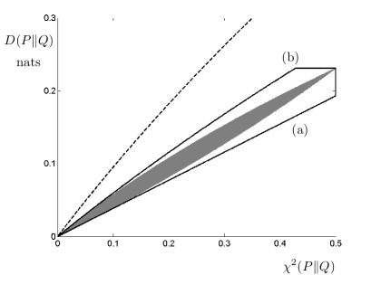
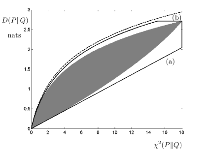
Figure 1: Comparison of the locus of the points $(\chi^{2}(P\|Q),D(P\|Q))$ when $P,Q$ are defined on $\mathcal{A}=\{0,1\}$ with the bounds in the left side of (188) (a) and Theorem 24 (b); $(\beta_{1},\beta_{2})=\bigl{(}\tfrac{1}{2},\tfrac{1}{2}\bigr{)}$ and $(\beta_{1},\beta_{2})=\bigl{(}\tfrac{1}{20},\tfrac{1}{20}\bigr{)}$ in the upper and lower plots, respectively. The dashed curve in each plot corresponds to the looser bound in (5).

The following result relies on the earlier analysis to provide bounds on the Bhattacharyya distance, expressed in terms of $\chi^{2}$ divergences and relative entropy.

Theorem 25

If $P\ll\gg Q$, then the following bounds on the Bhattacharyya distance hold:

$$\tfrac{1}{2}\log\bigl{(}1+\chi^{2}(P\|Q)\bigr{)}-\log\left(1+\tfrac{3}{4}\sqrt{\tfrac{\chi^{2}(P\|Q)}{2\log e}\Bigl{[}\log\bigl{(}1+\chi^{2}(P\|Q)\bigr{)}-D(P\|Q)\Bigr{]}}\right)$$

$$\leq B(P\|Q)$$ (348)

$$\leq\tfrac{1}{2}\log\bigl{(}1+\chi^{2}(P\|Q)\bigr{)}-\log\left(1+\frac{\bigl{(}\tfrac{3}{4}\,\chi^{2}(P\|Q)\bigr{)}^{\frac{3}{2}}}{\sqrt{\bigl{(}1+\chi^{2}(P\|Q)\bigr{)}^{2}\bigl{(}1+\chi^{2}(Q\|P)\bigr{)}-1}}\right).$$ (349)

Furthermore, if $\{P_{n}\}$ converges to $Q$ in the sense of (223), then the ratio of the bounds on $B(P_{n}\|Q)$ in (348) and (349) tends to 1 as $n\to\infty$.

Proof:

In view of the log-convexity of $\lambda_{\alpha}$ in $\alpha\in\mathbb{R}$,

$$\lambda_{0}\,\lambda_{-1}\geq\lambda_{-\frac{1}{2}}^{2},\quad\lambda_{-\frac{1}{2}}^{2}\,\lambda_{-2}\geq\lambda_{-1}^{3}$$ (350)

for any choice of the random variable $W$ in (315). Consequently, assembling (85), (316), (317) and (350) yield the bounds on $B(P\|Q)$ in (348) and (349).

Suppose that $\{P_{n}\}$ converges to $Q$ in the sense of (223). Let $L_{n}$ and $U_{n}$ denote, respectively, the lower and upper bounds on $B(P_{n}\|Q)$ in (348) and (349). Assembling (321)–(324), it can be easily verified that

$$\lim_{n\to\infty}\frac{L_{n}}{\chi^{2}(P_{n}\|Q)}=\lim_{n\to\infty}\frac{U_{n}}{\chi^{2}(P_{n}\|Q)}=\tfrac{1}{8}\,\log e$$ (351)

which yields that $\lim_{n\to\infty}\frac{U_{n}}{L_{n}}=1.$ ∎

Remark 25

Note that (349) refines the bound

$$B(P\|Q)\leq\tfrac{1}{2}\log\bigl{(}1+\chi^{2}(P\|Q)\bigr{)}$$ (352)

which is equivalent to $\lambda_{-\frac{1}{2}}\geq 0$ (in view of Jensen’s inequality, (85) and (317)).

Remark 26

Let $\{P_{n}\}$ converge to $Q$ in the sense of (223). In view of (351), it follows that

$$\lim_{n\to\infty}\frac{B(P_{n}\|Q)}{\chi^{2}(P_{n}\|Q)}=\tfrac{1}{8}\,\log e,$$ (353)

from which we can surmise that both upper bounds in (311) and (326) are tight under the condition in (223) (see Theorem 23), although (311) only depends on $\chi^{2}$-divergences. In view of (353), the lower bound in (329) is also tight under the condition in (223), in the sense that the ratio of $D(P_{n}\|Q)$ and its lower bound in (329) tends to 1 as $n\to\infty$; this sufficient condition for the tightness of (329) strengthens the result in [97, Section 4].

VI Reverse Pinsker Inequalities

It is not possible to lower bound $|P-Q|$ solely in terms of $D(P\|Q)$ since for any arbitrarily small $\epsilon>0$ and arbitrarily large $\lambda>0$, we can construct examples with $|P-Q|<\epsilon$ and $\lambda<D(P\|Q)<\infty$. Therefore, each of the bounds in this section involves not only $D(P\|Q)$ but another feature of the pair $(P,Q)$.

VI-A Bounded Relative Information

As in Section IV, the following result involves the bounds on the relative information.

Theorem 26

If $\beta_{1}\in(0,1)$ and $\beta_{2}\in[0,1)$, then,

$$D(P\|Q)\leq\tfrac{1}{2}\left(\varphi(\beta_{1}^{-1})-\varphi(\beta_{2})\right)\,|P-Q|$$ (354)

where $\varphi\colon[0,\infty)\to[0,\infty)$ is given by

$$\varphi(t)=\left\{\begin{array}[]{ll}0&t=0\\ \frac{t\log t}{t-1}&t\in(0,1)\cup(1,\infty)\\ \log e&t=1.\end{array}\right.$$ (358)

Proof:

Let $X\sim P$, $Y\sim Q$, and $Z$ be defined in (34). The function $\varphi\colon[0,\infty)\to[0,\infty)$ is continuous, monotonically increasing and non-negative; the monotonicity property holds since $(t-1)^{2}\varphi^{\prime}(t)=(t-1)\log e-\log t\geq 0$ for all $t>0$, and its non-negativity follows from the fact that $\varphi$ is monotonically increasing on $[0,\infty)$ and $\varphi(0)=0$. Accordingly,

$$\varphi(\beta_{2})\leq\varphi(Z)\leq\varphi(\beta_{1}^{-1})$$ (359)

since (34) and (153)–(154) imply that $Z\in[\beta_{2},\beta_{1}^{-1}]$ with probability one. The relative entropy satisfies

$$D(P\|Q) =\mathbb{E}\bigl{[}Z\log Z\bigr{]}$$ (360)

$$=\mathbb{E}\bigl{[}\varphi(Z)\,(Z-1)\bigr{]}$$ (361)

$$=\mathbb{E}\bigl{[}\varphi(Z)\,(Z-1)\,1\{Z>1\}\bigr{]}+\mathbb{E}\bigl{[}\varphi(Z)\,(Z-1)\,1\{Z<1\}\bigr{]}.$$ (362)

We bound each of the summands in the right side of (362) separately. Invoking (359), we have

$$\mathbb{E}\bigl{[}\varphi(Z)\,(Z-1)\,1\{Z>1\}\bigr{]} \leq\varphi(\beta_{1}^{-1})\,\mathbb{E}\bigl{[}(Z-1)\,1\{Z>1\}\bigr{]}$$ (363)

$$=\varphi(\beta_{1}^{-1})\,\mathbb{E}\bigl{[}(1-Z)^{-}\bigr{]}$$ (364)

$$=\tfrac{1}{2}\,\varphi(\beta_{1}^{-1})\,|P-Q|$$ (365)

where (364) holds since $(x)^{-}\triangleq-x\,1\{x<0\}$, and (365) follows from (262) with $Z$ in (34). Similarly, (359) yields

$$\mathbb{E}\bigl{[}\varphi(Z)\,(Z-1)\,1\{Z<1\}\bigr{]} \leq\varphi(\beta_{2})\,\mathbb{E}\bigl{[}(Z-1)\,1\{Z<1\}\bigr{]}$$ (366)

$$=-\varphi(\beta_{2})\,\mathbb{E}\bigl{[}(1-Z)^{+}\bigr{]}$$ (367)

$$=-\tfrac{1}{2}\,\varphi(\beta_{2})\,|P-Q|$$ (368)

where (368) follows from (261). Assembling (362), (365) and (368), we obtain (354). ∎

Remark 27

By dropping the negative term in (354), we can get the weaker version in [109, Theorem 7]:

$$D(P\|Q)\leq\left(\frac{\log\frac{1}{\beta_{1}}}{2(1-\beta_{1})}\right)|P-Q|.$$ (369)

The coefficient of $|P-Q|$ in the right side of (369) is monotonically decreasing in $\beta_{1}$ and it tends to $\tfrac{1}{2}\log e$ by letting $\beta_{1}\to 1$. The improvement over (369) afforded by (354) is exemplified in Appendix E. The bound in (369) has been recently used in the context of the optimal quantization of probability measures [12, Proposition 4].

Remark 28

The proof of Theorem 26 hinges on the fact that the function $\varphi$ is monotonically increasing. It can be verified that $\varphi$ is also concave and differentiable. Taking into account these additional properties of $\varphi$, the bound in Theorem 26 can be tightened as (see Appendix F):

$$D(P\|Q)\leq \tfrac{1}{2}\left(\varphi(\beta_{1}^{-1})-\varphi(\beta_{2})-\varphi^{\prime}(\beta_{1}^{-1})\;\beta_{1}^{-1}\right)\;|P-Q|+\varphi^{\prime}(\beta_{1}^{-1})\;\mathbb{E}\bigl{[}Z(Z-1)\,1\{Z>1\}\bigr{]}$$ (370)

which is expressed in terms of the distribution of the relative information. The second summand in the right side of (370) satisfies

$$\chi^{2}(P\|Q)+\tfrac{\beta_{2}}{2}\,|P-Q| \leq\mathbb{E}\bigl{[}Z(Z-1)\,1\{Z>1\}\bigr{]}$$ (371)

$$\leq\chi^{2}(P\|Q)+\tfrac{1}{2}|P-Q|.$$ (372)

From (34), (262) and $Z\in[\beta_{2},\beta_{1}^{-1}]$, the gap between the upper and lower bounds in (372) satisfies

$$\tfrac{1}{2}(1-\beta_{2})\,|P-Q| =(1-\beta_{2})\,\mathbb{E}\bigl{[}(1-Z)^{+}\bigr{]}$$ (373)

$$\leq(1-\beta_{2})^{2}$$ (374)

which is upper bounded by 1, and it is close to zero if $\beta_{2}\approx 1$. The combination of (370) and (372) leads to

$$D(P\|Q)\leq\tfrac{1}{2}\,\Bigl{(}\varphi(\beta_{1}^{-1})-\varphi(\beta_{2})+\varphi^{\prime}(\beta_{1}^{-1})\;\bigl{(}1-\beta_{1}^{-1}\bigr{)}\Bigr{)}\;|P-Q|+\varphi^{\prime}(\beta_{1}^{-1})\cdot\chi^{2}(P\|Q).$$ (375)

Remark 29

A special case of (369), where $Q$ is the uniform distribution over a set of a finite size, was recently rediscovered in [58, Corollary 13] based on results from [52].

Remark 30

For $\varepsilon\in[0,2]$ and a fixed probability measure $Q$, define

$$D^{*}(\varepsilon,Q)=\inf_{P\colon|P-Q|\geq\varepsilon}D(P\|Q).$$ (376)

From Sanov’s theorem (see [20, Theorem 11.4.1]), $D^{*}(\varepsilon,Q)$ is equal to the asymptotic exponential decay of the probability that the total variation distance between the empirical distribution of a sequence of i.i.d. random variables and the true distribution $Q$ is more than a specified value $\varepsilon$. Bounds on $D^{*}(\varepsilon,Q)$ have been shown in [10, Theorem 1], which, locally, behave quadratically in $\varepsilon$ . Although this result was classified in [10] as a reverse Pinsker inequality, note that it differs from the scope of this section which provides, under suitable conditions, lower bounds on the total variation distance as a function of the relative entropy.

VI-B Lipschitz Constraints

Definition 6

A function $f\colon\mathcal{B}\to\mathbb{R}$, where $\mathcal{B}\subseteq\mathbb{R}$, is $L$-Lipschitz if for all $x,y\in\mathcal{B}$

$$|f(x)-f(y)|\leq L\;|x-y|.$$ (377)

The following bound generalizes [35, Theorem 6] to the non-discrete setting.

Theorem 27

Let $P\ll Q$ with $\beta_{1}\in(0,1)$ and $\beta_{2}\in[0,1)$, and $f\colon[0,\infty)\to\mathbb{R}$ be continuous and convex with $f(1)=0$, and $L$-Lipschitz on $[\beta_{2},\beta_{1}^{-1}]$. Then,

$$D_{f}(P\|Q)\leq L\,|P-Q|.$$ (378)

Proof:

If $Y\sim Q$, and $Z$ is given by (34) then $f(1)=0$ yields

$$D_{f}(P\|Q) =\mathbb{E}\bigl{[}f(Z)\bigr{]}$$ (379)

$$\leq\mathbb{E}\bigl{[}\bigl{|}f(Z)-f(1)\bigr{|}\bigr{]}$$ (380)

$$\leq L\;\mathbb{E}\bigl{[}\bigl{|}Z-1\bigr{|}\bigr{]}$$ (381)

$$=L\;|P-Q|$$ (382)

where (382) holds due to (260). ∎

Note that if $f$ has a bounded derivative on $[\beta_{2},\beta_{1}^{-1}]$, we can choose

$$L=\sup_{t\in[\beta_{2},\beta_{1}^{-1}]}|f^{\prime}(t)|<\infty.$$ (383)

Remark 31

In the case $f(t)=t\log t$, $f(0)=0$, (383) particularizes to

$$L=\max\bigl{\{}\bigl{|}\log(e\beta_{2})\bigr{|},\,\log(e\beta_{1}^{-1})\bigr{\}}$$ (384)

resulting in a reverse Pinsker inequality which is weaker than that in (354) by at least a factor of 2.

VI-C Finite Alphabet

Throughout this subsection, we assume that $P$ and $Q$ are probability measures defined on a common finite set $\mathcal{A}$, and $Q$ is strictly positive on $\mathcal{A}$, which has more than one element.

The bound in (369) strengthens the finite-alphabet bound in [38, Lemma 3.10]:

$$D(P\|Q)\leq\log\left(\frac{1}{Q_{\min}}\right)\cdot|P-Q|$$ (385)

with

$$Q_{\min}=\min_{a\in\mathcal{A}}Q(a)\leq\tfrac{1}{2}.$$ (386)

To verify this, notice that $\beta_{1}\geq Q_{\min}$. Let $v\colon(0,1)\to(0,\infty)$ be defined by $v(t)=\frac{1}{1-t}\cdot\log\frac{1}{t}$; since $v$ is a monotonically decreasing and non-negative function, we can weaken (369) to write

$$D(P\|Q) \leq\left(\frac{\log\frac{1}{Q_{\min}}}{2(1-Q_{\min})}\right)|P-Q|$$ (387)

$$\leq\log\left(\frac{1}{Q_{\min}}\right)\cdot|P-Q|$$ (388)

where (388) follows from (386).

The main result in this subsection is the following bound.

Theorem 28

$$D(P\|Q)\leq\log\left(1+\frac{|P-Q|^{2}}{2Q_{\min}}\right).$$ (389)

Furthermore, if $Q\ll P$ and $\beta_{2}$ is defined as in (152), then the following tightened bound holds:

$$D(P\|Q) \leq\log\left(1+\frac{|P-Q|^{2}}{2Q_{\min}}\right)-\frac{\beta_{2}\log e}{2}\cdot|P-Q|^{2}.$$ (390)

Proof:

Combining (5) and the following finite-alphabet upper bound on $\chi^{2}(P\|Q)$ yields (389):

$$Q_{\min}\;\chi^{2}(P\|Q) =\sum_{a\in\mathcal{A}}\frac{(P(a)-Q(a))^{2}}{Q(a)/Q_{\min}}$$ (391)

$$\leq\sum_{a\in\mathcal{A}}\bigl{(}P(a)-Q(a)\bigr{)}^{2}$$ (392)

$$\leq\max_{x\in\mathcal{A}}|P(x)-Q(x)|\,\sum_{a\in\mathcal{A}}\bigl{|}P(a)-Q(a)\bigr{|}$$

$$=|P-Q|\;\max_{a\in\mathcal{A}}|P(a)-Q(a)|$$ (393)

$$\leq\tfrac{1}{2}\,|P-Q|^{2}.$$ (394)

If $P\ll\gg Q$, then (390) follows by combining (394) and

$$\chi^{2}(P\|Q) \geq\exp\Bigl{(}D(P\|Q)+\beta_{2}\,D(Q\|P)\Bigr{)}-1$$ (395)

$$\geq\exp\left(D(P\|Q)+\tfrac{1}{2}\,|P-Q|^{2}\,\beta_{2}\,\log e\right)-1$$ (396)

where (395) follows by rearranging (258), and (396) follows from (1). ∎

Remark 32

It is easy to check that Theorem 28 strengthens the bound by Csiszár and Talata (25) by at least a factor of 2 since upper bounding the logarithm in (389) gives

$$D(P\|Q)\leq\frac{\log e}{2Q_{\min}}\cdot{|P-Q|^{2}}.$$ (397)

Remark 33

In the finite-alphabet case, similarly to (389), one can obtain another upper bound on $D(P\|Q)$ as a function of the $\ell_{2}$ norm $\|P-Q\|_{2}$:

$$D(P\|Q)\leq\frac{1}{Q_{\min}}\cdot\|P-Q\|_{2}^{2}\,\log e$$ (398)

which appears in the proof of Property 4 of [100, Lemma 7], and also used in [57, (174)]. Furthermore, similarly to (390), the following tightened bound holds if $P\ll\gg Q$:

$$D(P\|Q)\leq\log\left(1+\frac{\|P-Q\|_{2}^{2}}{Q_{\min}}\right)-\frac{\beta_{2}\log e}{2}\cdot\|P-Q\|_{2}^{2}$$ (399)

which follows by combining (392), (396), and the inequality $\|P-Q\|_{2}\leq|P-Q|$.

Remark 34

Combining (1) and (394) yields that if $P\neq Q$ are defined on a common finite set, then

$$\frac{D(P\|Q)}{\chi^{2}(P\|Q)}\geq Q_{\min}\,\log e$$ (400)

which at least doubles the lower bound in [72, Lemma 6]. This, in turn, improves the tightened upper bound on the strong data processing inequality constant in [72, Theorem 10] by a factor of 2.

Remark 35

Reverse Pinsker inequalities have been also derived in quantum information theory ([3, 4]), providing upper bounds on the relative entropy of two quantum states as a function of the trace norm distance when the minimal eigenvalues of the states are positive (c.f. [3, Theorem 6] and [4, Theorem 1]). When the variational distance is much smaller than the minimal eigenvalue (see [3, Eq. (57)]), the latter bounds have a quadratic scaling in this distance, similarly to (389); they are also inversely proportional to the minimal eigenvalue, similarly to the dependence of (389) in $Q_{\min}$.

Remark 36

Let $P$ and $Q$ be probability distributions defined on an arbitrary alphabet $\mathcal{A}$. Combining Theorems 7 and 26 leads to a derivation of an upper bound on the difference $D(P\|Q)-D(Q\|P)$ as a function of $|P-Q|$ as long as $P\ll\gg Q$ and the relative information $\imath_{P\|Q}$ is bounded away from $-\infty$ and $+\infty$. Furthermore, another upper bound on the difference of the relative entropies can be readily obtained by combining Theorems 7 and 28 when $P$ and $Q$ are probability measures defined on a finite alphabet. In the latter case, combining Theorem 7 and (399) also yields another upper bound on $D(P\|Q)-D(Q\|P)$ which scales quadratically with $\|P-Q\|_{2}$. All these bounds form a counterpart to [5, Theorem 1] and Theorem 7, providing measures of the asymmetry of the relative entropy when the relative information is bounded.

VI-D Distance From the Equiprobable Distribution

If $P$ is a distribution on a finite set $\mathcal{A}$, $H(P)$ gauges the “distance” from $\mathsf{U}$, the equiprobable distribution defined on $\mathcal{A}$, since $H(P)=\log|\mathcal{A}|-D(P\|\mathsf{U})$. Thus, it is of interest to explore the relationship between $H(P)$ and $|P-\mathsf{U}|$. Next, we determine the exact locus of the points $(H(P),\,|P-\mathsf{U}|)$ among all probability measures $P$ defined on $\mathcal{A}$, and this region is compared to upper and lower bounds on $|P-\mathsf{U}|$ as a function of $H(P)$. As usual, $h(x)$ denotes the continuous extension of $-x\log x-(1-x)\log(1-x)$ to $x\in[0,1]$ and $d(x\|y)$ denotes the binary relative entropy in (332).

Theorem 29

Let $\mathsf{U}$ be the equiprobable distribution on a $\{1,\ldots,|\mathcal{A}|\}$, with $1<|\mathcal{A}|<\infty$.

1. For $\Delta\in(0,2(1-|\mathcal{A}|^{-1})]$,

   $$\max_{P\colon|P-\mathsf{U}|=\Delta}H(P)=\log|\mathcal{A}|-\min_{m}\,d\left(\tfrac{m}{|\mathcal{A}|}+\tfrac{1}{2}\Delta\,\big{\|}\,\tfrac{m}{|\mathcal{A}|}\right)$$ (401)

   where the minimum in the right side of (401) is over

   $$m\in\{1,\ldots,|\mathcal{A}|-\bigl{\lceil}\tfrac{1}{2}\Delta|\mathcal{A}|\bigr{\rceil}\}.$$ (402)

   Denoting such an integer by $m_{\Delta}$, the maximum in the left side of (401) is attained by

   $$P_{\Delta}(\ell)=\left\{\begin{array}[]{ll}|\mathcal{A}|^{-1}+\frac{\Delta}{2m_{\Delta}}&\ell\in\{1,\ldots,m_{\Delta}\},\\[5.69046pt] |\mathcal{A}|^{-1}-\frac{\Delta}{2(|\mathcal{A}|-m_{\Delta})},&\ell\in\{m_{\Delta}+1,\ldots,|\mathcal{A}|\}.\end{array}\right.$$ (405)

2. Let

   $$h_{k}=\left\{\begin{array}[]{ll}0,&k=0\\[2.84544pt] h\bigl{(}|\mathcal{A}|^{-1}k\bigr{)}+|\mathcal{A}|^{-1}\,k\log k,&k\in\{1,\ldots,|\mathcal{A}|-2\}\\[2.84544pt] \log|\mathcal{A}|,&k=|\mathcal{A}|-1.\end{array}\right.$$ (409)

   If $H\in[h_{k-1},h_{k})$ for $k\in\{1,\ldots,|\mathcal{A}|-1\}$, then

   $$\min_{P\colon H(P)=H}|P-\mathsf{U}|=2\bigl{(}1-(k+\theta)\,|\mathcal{A}|^{-1}\bigr{)}$$ (410)

   which is achieved by

   $$P^{(k)}_{\theta}(\ell)=\left\{\begin{array}[]{ll}1-(k-1+\theta)\,|\mathcal{A}|^{-1},&\ell=1\\[2.84544pt] |\mathcal{A}|^{-1},&\ell\in\{2,\ldots,k\},\\[2.84544pt] \theta\,|\mathcal{A}|^{-1},&\ell=k+1\\[2.84544pt] 0,&\ell\in\{k+2,\ldots,|\mathcal{A}|\}\end{array}\right.$$ (415)

   where $\theta\in[0,1)$ is chosen so that $H(P^{(k)}_{\theta})=H$.

Proof:

See Appendix G. ∎

Remark 37

For probability measures defined on a 2-element set $\mathcal{A}$, the maximal and minimal values of $|P-\mathsf{U}|$ in Theorem 29 coincide. This can be verified since, if $P(1)=p$ for $p\in[0,1]$, then $|P-\mathsf{U}|=|1-2p|$ and $H(P)=h(p)$. Hence, if $|\mathcal{A}|=2$ and $H(P)=H\in[0,\log 2]$, then

$$|P-\mathsf{U}|=1-2h^{-1}(H)$$ (416)

where $h^{-1}\colon[0,\log 2]\to[0,\tfrac{1}{2}]$ denotes the inverse of the binary entropy function.

Results on the more general problem of finding bounds on $|H(P)-H(Q)|$ based on $|P-Q|$ can be found in [20, Theorem 17.3.3], [52], [90] and [113]. Most well-known among them is

$$|H(P)-H(Q)|\leq|P-Q|\log\left(\frac{|\mathcal{A}|}{|P-Q|}\right)$$ (417)

which holds if $P,Q$ are probability measures defined on a finite set $\mathcal{A}$ with $\bigl{|}P(a)-Q(a)\bigr{|}\leq\frac{1}{2}$ for all $a\in\mathcal{A}$ (see [110], and [27, Lemma 2.7] with a stronger sufficient condition). Particularizing (417) to the case where $Q=\mathsf{U}$, and $\left|P(a)-\tfrac{1}{|\mathcal{A}|}\right|\leq\tfrac{1}{2}$ for all $a\in\mathcal{A}$ yields

$$H(P)\geq\log|\mathcal{A}|-|P-\mathsf{U}|\,\log\left(\frac{|\mathcal{A}|}{|P-\mathsf{U}|}\right),$$ (418)

a bound which finds use in information-theoretic security [30].

Particularizing (1), (4), and (389) we obtain

$$H(P) \leq\log|\mathcal{A}|-\tfrac{1}{2}\,|P-\mathsf{U}|^{2}\,\log e,$$ (419)

$$H(P) \leq\log|\mathcal{A}|+\log\left(1-\tfrac{1}{4}\,|P-\mathsf{U}|^{2}\right),$$ (420)

$$H(P) \geq\log|\mathcal{A}|-\log\left(1+\tfrac{|\mathcal{A}|}{2}\;|P-\mathsf{U}|^{2}\right).$$ (421)

If either $|\mathcal{A}|=2$ or $8\leq|\mathcal{A}|\leq 102$, it can be checked that the lower bound on $H(P)$ in (418) is worse than (421), irrespectively of $|P-\mathsf{U}|$ (note that $0\leq|P-\mathsf{U}|\leq 2(1-|\mathcal{A}|^{-1})$).

The exact locus of $(H(P),|P-\mathsf{U}|)$ among all the probability measures $P$ defined on a finite set $\mathcal{A}$ (see Theorem 29), and the bounds in (419)–(421) are illustrated in Figure 2 for $|\mathcal{A}|=4$ and $|\mathcal{A}|=256$. For $|\mathcal{A}|=4$, the lower bound in (421) is tighter than (418). For $|\mathcal{A}|=256$, we only show (421) in Figure 2 as in this case (418) offers a very minor improvement in a small range. As the cardinality of the set $\mathcal{A}$ increases, the gap between the exact locus (shaded region) and the upper bound obtained from (419) and (420) (Curves (a) and (b), respectively) decreases, whereas the gap between the exact locus and the lower bound in (421) (Curve (c)) increases.

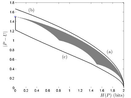
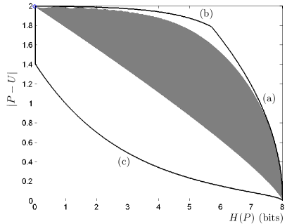
Figure 2: The exact locus of $(H(P),|P-\mathsf{U}|)$ among all the probability measures $P$ defined on a finite set $\mathcal{A}$, and bounds on $|P-\mathsf{U}|$ as a function of $H(P)$ for $|\mathcal{A}|=4$ (left plot), and $|\mathcal{A}|=256$ (right plot). The point $(H(P),|P-\mathsf{U}|)=(0,\,2(1-|\mathcal{A}|^{-1}))$ is depicted on the $y$-axis. In the two plots, Curves (a), (b) and (c) refer, respectively, to (419), (420) and (421); the exact locus (shaded region) refers to Theorem 29.

VI-E The Exponential Decay of the Probability of Non-Strongly Typical Sequences

The objective is to bound the function

$$L_{\delta}(Q)=\min_{P\not\in\mathcal{T}_{\delta}(Q)}D(P\|Q)$$ (422)

where the subset of probability measures on $(\mathcal{A},\mathscr{F})$ which are $\delta$-close to $Q$ is given by

$$\mathcal{T}_{\delta}(Q)=\Bigl{\{}P\colon\forall\,a\in\mathcal{A},\;\;|P(a)-Q(a)|\leq\delta\,Q(a)\Bigr{\}}.$$ (423)

Note that $(a_{1},\ldots,a_{n})$ is strongly $\delta$-typical according to $Q$ if its empirical distribution belongs to $\mathcal{T}_{\delta}(Q)$. According to Sanov’s theorem (e.g. [20, Theorem 11.4.1]), if the random variables are independent and distributed according to $Q$, then the probability that $(Y_{1},\ldots,Y_{n})$, is not $\delta$-typical vanishes exponentially with exponent $L_{\delta}(Q)$.

To state the next result, we invoke the following notions from [76]. Given a probability measure $Q$, its balance coefficient is given by

$$\beta_{Q}=\inf_{\mathcal{F}\in\mathscr{F}\colon Q(\mathcal{F})\geq\frac{1}{2}}Q(\mathcal{F}).$$ (424)

The function $\phi\colon(0,\tfrac{1}{2}]\to[\tfrac{1}{2}\log e,\infty)$ is a monotonically decreasing and convex function, which is given by

$$\phi(p)=\left\{\begin{array}[]{ll}\frac{1}{4(1-2p)}\,\log\left(\frac{1-p}{p}\right),&p\in\bigl{(}0,\tfrac{1}{2}\bigr{)},\\[2.84544pt] \tfrac{1}{2}\log e,&p=\tfrac{1}{2}.\end{array}\right.$$ (427)

Theorem 30

If $Q_{\min}>0$, then

$$\phi(1-\beta_{Q})\,Q_{\min}^{2}\,\delta^{2} \leq L_{\delta}(Q)$$ (428)

$$\leq\log\left(1+2Q_{\min}\,\delta^{2}\right)$$ (429)

where (429) holds if $\delta<\frac{1-Q_{\max}}{Q_{\min}}$.

Proof:

The following refinement of Pinsker’s inequality (1) was derived in [76, Section 4]:

$$\phi(1-\beta_{Q})\;|P-Q|^{2}\leq D(P\|Q).$$ (430)

Note that if $Q_{\min}>0$ then $\beta_{Q}\leq 1-Q_{\min}<1$, and $\phi(1-\beta_{Q})$ is well defined and finite. If $P\not\in\mathcal{T}_{\delta}(Q)$, the simple bound

$$|P-Q|>\delta Q_{\min}$$ (431)

together with (422) and (430) yields (428).

The upper bound (429) follows from (389) and the fact that if $\delta<\frac{1-Q_{\max}}{Q_{\min}}$, then

$$\inf_{P\not\in\mathcal{T}_{\delta}(Q)}|P-Q|=2\delta Q_{\min}.$$ (432)

To verify (432), note that for every $P\not\in\mathcal{T}_{\delta}(Q)$, there exists $a\in\mathcal{A}$ such that $|P(a)-Q(a)|>\delta\,Q(a)$, which implies that $|P-Q|>2\delta\,Q(a)\geq 2\delta Q_{\min}$, thereby establishing $\geq$ in (432). To show equality, let $a_{0}\in\mathcal{A}$ be such that $Q(a_{0})=Q_{\min}$, and let $a_{1}\neq a_{0}$; since by assumption $\delta<\frac{1-Q_{\max}}{Q_{\min}}$, we have $Q(a_{1})+\delta\,Q_{\min}\leq Q_{\max}+\delta\,Q_{\min}<1$. Let

$$P(a)=\left\{\begin{array}[]{ll}(1-\delta-\varepsilon)\,Q_{\min}&a=a_{0}\\ Q(a_{1})+(\delta+\varepsilon)\,Q_{\min}&a=a_{1}\\ Q(a)&\mbox{otherwise}\end{array}\right.$$ (436)

for a sufficiently small $\varepsilon>0$ so that (436) is a probability measure. Then, $P\not\in\mathcal{T}_{\delta}(Q)$ and $|P-Q|=2(\delta+\varepsilon)\,Q_{\min}$, which verifies the equality in (432) by letting $\varepsilon\downarrow 0$. ∎

Remark 38

If $\delta<\frac{1-Q_{\max}}{Q_{\min}}$, the ratio between the upper and lower bounds in (429), satisfies

$$\frac{1}{Q_{\min}}\cdot\frac{\log e}{2\,\phi(1-\beta_{Q})}\cdot\frac{\log\left(1+2Q_{\min}\,\delta^{2}\right)}{\tfrac{1}{2}\,Q_{\min}\,\delta^{2}\,\log e}\leq\frac{4}{Q_{\min}}$$ (437)

where (437) follows from the fact that its second and third factors are less than or equal to 1 and 4, respectively. Note that both bounds in (429) scale like $\delta^{2}$ for $\delta\approx 0$.

VII The $E_{\gamma}$ Divergence

VII-A Basic Properties

Generalizing the total variation distance, the $E_{\gamma}$ divergence in (68) is an $f$-divergence whose utility in information theory has been exemplified in [18], [68], [69], [70], [79],[80], [81].

In this subsection, we provide some basic properties of the $E_{\gamma}$ divergence, which are essential to Sections VII-B–VII-D. The reader is referred to [68, Sections 2.B, 2.C] for some additional basic properties of the $E_{\gamma}$ divergence. We assume throughout this section that $\gamma\geq 1$.

Let $P\ll Q$. The $E_{\gamma}$ divergence in (68) can be expressed in the form

$$E_{\gamma}(P\|Q) =\mathbb{P}\bigl{[}\imath_{P\|Q}(X)>\log\gamma\bigr{]}-\gamma\,\mathbb{P}\bigl{[}\imath_{P\|Q}(Y)>\log\gamma\bigr{]}$$ (438)

$$=\max_{\mathcal{F}\in\mathscr{F}}\bigl{(}P(\mathcal{F})-\gamma\,Q(\mathcal{F})\bigr{)}$$ (439)

where $X\sim P$ and $Y\sim Q$, and (439) follows from the Neyman-Pearson lemma.

Although the $E_{\gamma}$ divergence generalizes the total variation distance, $E_{\gamma}(P\|Q)=0$ for $\gamma>1$ does not imply $P=Q$ since in that case (69) is not strictly convex at $t=1$ (see Proposition 1). This is illustrated in the following example.

Example 13

Let $\gamma>1$, and let $P$ and $Q$ be probability measures defined on $\mathcal{A}=\{0,1\}$:

$$P(0)=\frac{1+\gamma}{2\gamma},\quad Q(0)=\frac{1}{\gamma}.$$ (440)

Since $\imath_{P\|Q}(x)=\log\gamma\;1\{x=0\}-\log 2<\log\gamma$ for all $x\in\mathcal{A}$, (438) implies that $E_{\gamma}(P\|Q)=0$.

The monotonicity of the $E_{\gamma}$ divergence in $\gamma\in[1,\infty)$ holds since $f_{\gamma_{1}}(t)\leq f_{\gamma_{2}}(t)$ for all $t>0$ with $f_{\gamma}(t)=(t-\gamma)^{+}$ and $\gamma_{1}\geq\gamma_{2}\geq 1$. Therefore,

$$\frac{E_{\gamma_{1}}(P\|Q)}{E_{\gamma_{2}}(P\|Q)}\leq 1.$$ (441)

Although Theorem 1b) does not apply in order to prove that $1$ is the best constant in (441), we can verify it by defining $P$ and $Q$ on $\mathcal{A}=\{0,1\}$ with $P(0)=\tfrac{1}{2}$ and $Q(0)=\varepsilon>0$. This yields that if $\gamma_{1}\geq\gamma_{2}\geq 1$, then for all $\varepsilon\in(0,\frac{1}{2\gamma_{1}})$,

$$\frac{E_{\gamma_{1}}(P\|Q)}{E_{\gamma_{2}}(P\|Q)}=\frac{1-2\varepsilon\gamma_{1}}{1-2\varepsilon\gamma_{2}},$$ (442)

yielding the optimality of the constant in the right side of (441) by letting $\varepsilon\downarrow 0$ in (442).

From (439), the following inequality holds: If $P\ll R\ll Q$, and $\gamma_{1},\gamma_{2}\geq 1$ then

$$E_{\gamma_{1}\gamma_{2}}(P\|Q)\leq E_{\gamma_{1}}(P\|R)+\gamma_{1}\,E_{\gamma_{2}}(R\|Q).$$ (443)

Letting $\gamma_{1}=1$ in (443) (see (70)) and $\gamma_{2}=\gamma$ yield

$$E_{\gamma}(P\|Q)-E_{\gamma}(R\|Q)\leq\tfrac{1}{2}|P-R|.$$ (444)

Generalizing the fact that $E_{1}(P\|Q)=\tfrac{1}{2}|P-Q|$, the following identity is a special case of [47, Corollary 2.3]:

$$\min_{R:P,Q\ll R}\Bigl{\{}E_{\gamma}(P\|R)+E_{\gamma}(Q\|R)\Bigr{\}}=\left(1-\gamma+\tfrac{1}{2}{|P-Q|}\right)^{+}$$ (445)

while [68, (21)] states that

$$\min_{R\ll P,Q}\Bigl{\{}E_{\gamma}(R\|P)+E_{\gamma}(R\|Q)\Bigr{\}}\geq\left(1-\gamma+\tfrac{\gamma}{2}\,|P-Q|\right)^{+},$$ (446)

which implies, by taking $R=P$,

$$\left(1-\gamma+\tfrac{\gamma}{2}\,|P-Q|\right)^{+}\leq E_{\gamma}(P\|Q).$$ (447)

We end this subsection with the following result.

Theorem 31

If $P\ll Q$ and $Y\sim Q$, then

$$\mathbb{E}\left[\bigl{|}\exp\bigl{(}\imath_{P\|Q}(Y)\bigr{)}-\gamma\bigr{|}\right] =2E_{\gamma}(P\|Q)+\gamma-1,$$ (448)

$$\mathbb{E}\left[\max\bigl{\{}\gamma,\,\exp\bigl{(}\imath_{P\|Q}(Y)\bigr{)}\bigr{\}}\right] =\gamma+E_{\gamma}(P\|Q),$$ (449)

$$\mathbb{E}\left[\min\bigl{\{}\gamma,\,\exp\bigl{(}\imath_{P\|Q}(Y)\bigr{)}\bigr{\}}\right] =1-E_{\gamma}(P\|Q).$$ (450)

Proof:

The identity $|z|=2(z)^{+}-z$, for all $z\in\mathbb{R}$, and (68) are used to prove (448):

$$\mathbb{E}\left[\bigl{|}\exp\bigl{(}\imath_{P\|Q}(Y)\bigr{)}-\gamma\bigr{|}\right] =2\mathbb{E}\left[\bigl{(}\exp\bigl{(}\imath_{P\|Q}(Y)\bigr{)}-\gamma\bigr{)}^{+}\right]-\mathbb{E}\left[\exp\bigl{(}\imath_{P\|Q}(Y)\bigr{)}-\gamma\right]$$ (451)

$$=2E_{\gamma}(P\|Q)+\gamma-1.$$ (452)

Eqs. (449) and (450) follow from (448), and the identities

$$\max\{x_{1},x_{2}\}=\tfrac{1}{2}\bigl{[}x_{1}+x_{2}+|x_{1}-x_{2}|\bigr{]},$$ (453)

$$\min\{x_{1},x_{2}\}=\,\tfrac{1}{2}\bigl{[}x_{1}+x_{2}-|x_{1}-x_{2}|\bigr{]}$$ (454)

for all $x_{1},x_{2}\in\mathbb{R}$. ∎

Remark 39

In view of (70), it follows that (448) and (449) are specialized respectively to (260) and [49, (20)] by letting $\gamma=1$.

VII-B An Integral Representation of $f$-divergences

In this subsection we show that

$$\bigl{\{}(E_{\gamma}(P\|Q),E_{\gamma}(Q\|P)),\gamma\geq 1\bigr{\}}$$

uniquely determines $D(P\|Q)$, $\mathscr{H}_{\alpha}(P\|Q)$, as well as any other $f$-divergence with twice differentiable $f$.

Proposition 3

Let $P\ll\gg Q$, and let $f\colon(0,\infty)\to\mathbb{R}$ be convex and twice differentiable with $f(1)=0$. Then,

$$D_{f}(P\|Q)=\int_{1}^{\infty} \bigr{(}f^{\prime\prime}(\gamma)\,E_{\gamma}(P\|Q)+\gamma^{-3}f^{\prime\prime}(\gamma^{-1})\,E_{\gamma}(Q\|P)\bigr{)}\,\text{d}\gamma.$$ (455)

Proof:

From [66, Theorem 11], if $f\colon(0,\infty)\to\mathbb{R}$ is a convex function with $f(1)=0$, then

$$D_{f}(P\|Q)=\int_{0}^{1}\mathcal{I}_{p}(P\|Q)\,\text{d}\Gamma_{f}(p)$$ (456)

where $\Gamma_{f}$ is the $\sigma$-finite measure defined on Borel subsets of $(0,1)$ by

$$\Gamma_{f}\bigl{(}(p_{1},p_{2}]\bigr{)}=\int_{p_{1}}^{p_{2}}\frac{1}{p}\,\text{d}g_{f}(p)$$ (457)

for the non-decreasing function

$$g_{f}(p)=-f^{\prime}_{+}\left(\frac{1-p}{p}\right),\quad p\in(0,1)$$ (458)

where $f^{\prime}_{+}$ denotes the right derivative of $f$.

The DeGroot statistical information in (71) has the following operational role [31], which is used in this proof. Assume hypotheses $H_{0}$ and $H_{1}$ have a-priori probabilities $p$ and $1-p$, respectively, and let $P$ and $Q$ be the conditional probability measures of an observation $Y$ given $H_{0}$ or $H_{1}$. Then, $\mathcal{I}_{p}(P\|Q)$ is equal to the difference between the minimum error probabilities when the most likely a-priori hypothesis is selected, and when the most likely a posteriori hypothesis is selected. This measure therefore quantifies the value of the observations for the task of discriminating between the hypotheses. From the operational role of this measure, it follows that if $P\ll\gg Q$

$$\mathcal{I}_{p}(P\|Q)=\mathcal{I}_{1-p}(Q\|P).$$ (459)

The $E_{\gamma}$ divergence and DeGroot statistical information are related by

$$\mathcal{I}_{p}(P\|Q)=\left\{\begin{array}[]{ll}pE_{\frac{1-p}{p}}(P\|Q),&\quad\mbox{$p\in\bigl{(}0,\tfrac{1}{2}]$}\\[5.69046pt] (1-p)E_{\frac{p}{1-p}}(Q\|P),&\quad\mbox{$p\in\bigl{[}\tfrac{1}{2},1)$.}\end{array}\right.$$ (462)

The expression for $p\in\bigl{(}0,\tfrac{1}{2}]$ follows from the fact that the functions that yield $E_{\gamma}$ and $\mathcal{I}_{p}$ in (69) and (72), respectively, satisfy

$$\phi_{p}=pf_{\frac{1-p}{p}}.$$ (463)

The remainder of (462) follows in view of (459).

Specializing (456) to a twice differentiable $f$ gives

$$D_{f}(P\|Q) =\int_{0}^{1}\mathcal{I}_{p}(P\|Q)\cdot\frac{1}{p^{3}}\,f^{\prime\prime}\left(\frac{1-p}{p}\right)\,\text{d}p$$ (464)

$$=\int_{0}^{\frac{1}{2}}\mathcal{I}_{p}(P\|Q)\cdot\frac{1}{p^{3}}\,f^{\prime\prime}\left(\frac{1-p}{p}\right)\,\text{d}p+\int_{\frac{1}{2}}^{1}\mathcal{I}_{p}(P\|Q)\cdot\frac{1}{p^{3}}\,f^{\prime\prime}\left(\frac{1-p}{p}\right)\,\text{d}p$$ (465)

$$=\int_{0}^{\frac{1}{2}}E_{\frac{1-p}{p}}(P\|Q)\cdot\frac{1}{p^{2}}\,f^{\prime\prime}\left(\frac{1-p}{p}\right)\,\text{d}p+\int_{\frac{1}{2}}^{1}E_{\frac{p}{1-p}}(Q\|P)\cdot\frac{1-p}{p^{3}}\,f^{\prime\prime}\left(\frac{1-p}{p}\right)\,\text{d}p$$ (466)

$$=\int_{1}^{\infty}E_{\gamma}(P\|Q)\,f^{\prime\prime}(\gamma)\,\text{d}\gamma+\int_{0}^{1}\gamma E_{\gamma^{-1}}(Q\|P)\,f^{\prime\prime}(\gamma)\,\text{d}\gamma$$ (467)

$$=\int_{1}^{\infty}\Bigl{[}f^{\prime\prime}(\gamma)\,E_{\gamma}(P\|Q)+\gamma^{-3}\,f^{\prime\prime}(\gamma^{-1})\,E_{\gamma}(Q\|P)\Bigr{]}\,\text{d}\gamma$$ (468)

where (464) follows from (456)–(458); (465) follows by splitting the interval of integration into two parts; (466) follows from (462); (467) follows by the substitution $\gamma=\tfrac{1-p}{p}$, and (468) follows by changing the variable of integration $t=\frac{1}{\gamma}$ in the second integral in (467). ∎

Particularizing Proposition 3 to the most salient $f$-divergences we obtain (cf. [66, (84)–(86)] for alternative integral representations as a function of DeGroot statistical information)

$$D(P\|Q) =\log e\,\int_{1}^{\infty}\left(\gamma^{-1}{E_{\gamma}(P\|Q)}+\gamma^{-2}{E_{\gamma}(Q\|P)}\right)\,\text{d}\gamma,$$ (469)

$$\mathscr{H}_{\alpha}(P\|Q) =\alpha\int_{1}^{\infty}\left(\gamma^{\alpha-2}\,E_{\gamma}(P\|Q)+\gamma^{-\alpha-1}\,E_{\gamma}(Q\|P)\right)\,\text{d}\gamma,$$ (470)

and specializing (470) to $\alpha=2$ yields

$$\chi^{2}(P\|Q) =2\int_{1}^{\infty}\left(\,E_{\gamma}(P\|Q)+\gamma^{-3}E_{\gamma}(Q\|P)\right)\,\text{d}\gamma.$$ (471)

Accordingly, bounds on the $E_{\gamma}$ divergence, such as those presented in Section VII-C, directly translate into bounds on other important $f$-divergences.

Remark 40

Proposition 3 can be derived also from the integral representation of $f$-divergences in [18, Corollary 3.7].

VII-C Extension of Pinsker’s Inequality to $E_{\gamma}$ Divergence

This subsection upper bounds $E_{\gamma}$ divergence in terms of the relative entropy.

Theorem 32

$$E_{\gamma}(P\|Q)\,{\log\gamma} \leq D(P\|Q)+2e^{-1}\log e,$$ (472)

$$2\,E_{\gamma}^{2}(P\|Q)\,\log e \leq D(P\|Q).$$ (473)

Proof:

The bound in (472) appears in [68, Proposition 13]. For $\gamma=1$, (473) reduces to (1). Since $E_{\gamma}$ is monotonically decreasing in $\gamma$, (473) also holds for $\gamma>1$. ∎

For $\gamma=1$, (473) becomes Pinsker’s inequality (1), for which there is no tighter constant. Moreover, in view of (70), for small $E_{1}(P\|Q)$, the minimum achievable $D(P\|Q)$ is indeed quadratic in $E_{1}(P\|Q)$ [39]. This ceases to be the case for $\gamma>1$, in which case it is possible to upper bound $E_{\gamma}(P\|Q)$ as a constant times $D(P\|Q)$.

Theorem 33

For every $\gamma>1$,

$$\sup\frac{E_{\gamma}(P\|Q)}{D(P\|Q)}=c_{\gamma}$$ (474)

where the supremum is over $P\ll Q,P\neq Q$, and $c_{\gamma}$ is a universal function (independent of $P$ and $Q$), given by

$$c_{\gamma}=\frac{t_{\gamma}-\gamma}{r(t_{\gamma})},$$ (475)

$$t_{\gamma}=-\gamma\,W_{-1}\left(-\tfrac{1}{\gamma}\,e^{-\frac{1}{\gamma}}\right)$$ (476)

with $r$ in (475) is given in (45), and $W_{-1}$ in (476) denotes the secondary real branch of the Lambert $W$ function [19].

Proof:

The functions $f_{\gamma}(t)=(t-\gamma)^{+}$ and $r$ (see (45)) satisfy the sufficient conditions of Theorem 1. Their ratio is

$$\kappa_{\gamma}(t) =\left\{\begin{array}[]{ll}\frac{t-\gamma}{r(t)}&t\in[\gamma,\infty)\\ 0&t\in(0,\gamma].\end{array}\right.$$ (479)

For $t>\gamma$

$$\kappa_{\gamma}^{\prime}(t)=\frac{\gamma\log t+(1-t)\log e}{r^{2}(t)}.$$ (480)

Since $\gamma>1$, it follows from (480) that there exists $t_{\gamma}\in(\gamma,\infty)$ such that $\kappa_{\gamma}$ is monotonically increasing on $[\gamma,t_{\gamma}]$, and it is monotonically decreasing on $[t_{\gamma},\infty)$. The value $t_{\gamma}$ is the unique solution of the equation $\kappa_{\gamma}^{\prime}(t)=0$ in $(\gamma,\infty)$. From (480), $t_{\gamma}\in(\gamma,\infty)$ solves the equation

$$\gamma\log t=(t-1)\,\log e$$ (481)

which, after exponentiating both sides of (481) and making the substitution $x=-\frac{t}{\gamma}$, gives

$$xe^{x}=-\tfrac{1}{\gamma}\,e^{-\frac{1}{\gamma}}.$$ (482)

The trivial solution of (482) $x=-\frac{1}{\gamma}$ corresponds to $t=1$, which is an improper solution of (481) since $t<\gamma$. The proper solution of (482) is its second real solution given by

$$x=W_{-1}\left(-\tfrac{1}{\gamma}\,e^{-\frac{1}{\gamma}}\right);$$ (483)

consequently, $t=-\gamma x$ and (483) give (476). In conclusion, for $t\geq 0$ and $\gamma>1$,

$$0\leq\kappa_{\gamma}(t)\leq\kappa_{\gamma}(t_{\gamma})=c_{\gamma}$$ (484)

where the equality in (484) follows from (475), (479), and $t_{\gamma}>\gamma$. Theorem 1a) yields

$$E_{\gamma}(P\|Q)\leq c_{\gamma}D(P\|Q).$$ (485)

To show (474), or in other words that there is no better constant in (485) than $c_{\gamma}$, it is enough to restrict to binary alphabets: Let $\mathcal{A}=\{0,1\}$, $\varepsilon\in(0,1)$, and $P_{\varepsilon}(0)=\varepsilon$, $Q_{\varepsilon}(0)=\frac{\varepsilon}{t_{\gamma}}$. Since $t_{\gamma}>1$, we have

$$\frac{P_{\varepsilon}(1)}{Q_{\varepsilon}(1)}=\frac{1-\varepsilon}{1-\frac{\varepsilon}{t_{\gamma}}}<1<\gamma$$ (486)

and

$$\kappa_{\gamma}\left(\frac{P_{\varepsilon}(1)}{Q_{\varepsilon}(1)}\right)=0$$ (487)

where (487) follows from (479) and (486). We show in the following that $\frac{E_{\gamma}(P_{\varepsilon}\|Q_{\varepsilon})}{D(P_{\varepsilon}\|Q_{\varepsilon})}$ can come arbitrarily close (from below) to $c_{\gamma}$ by choosing a sufficiently small $\varepsilon>0$. To that end, for all $\varepsilon\in(0,1)$,

$$E_{\gamma}(P_{\varepsilon}\|Q_{\varepsilon}) =Q_{\varepsilon}(0)\;f_{\gamma}\left(\frac{P_{\varepsilon}(0)}{Q_{\varepsilon}(0)}\right)+Q_{\varepsilon}(1)\;f_{\gamma}\left(\frac{P_{\varepsilon}(1)}{Q_{\varepsilon}(1)}\right)$$ (488)

$$=Q_{\varepsilon}(0)\;r\left(\frac{P_{\varepsilon}(0)}{Q_{\varepsilon}(0)}\right)\;\kappa_{\gamma}\left(\frac{P_{\varepsilon}(0)}{Q_{\varepsilon}(0)}\right)+Q_{\varepsilon}(1)\;r\left(\frac{P_{\varepsilon}(1)}{Q_{\varepsilon}(1)}\right)\;\kappa_{\gamma}\left(\frac{P_{\varepsilon}(1)}{Q_{\varepsilon}(1)}\right)$$ (489)

$$=Q_{\varepsilon}(0)\;r\left(\frac{P_{\varepsilon}(0)}{Q_{\varepsilon}(0)}\right)\;\kappa_{\gamma}\left(\frac{P_{\varepsilon}(0)}{Q_{\varepsilon}(0)}\right)$$ (490)

$$=c_{\gamma}\;Q_{\varepsilon}(0)\;r\left(\frac{P_{\varepsilon}(0)}{Q_{\varepsilon}(0)}\right)$$ (491)

$$=c_{\gamma}\left[D(P_{\varepsilon}\|Q_{\varepsilon})-Q_{\varepsilon}(1)\;r\left(\frac{P_{\varepsilon}(1)}{Q_{\varepsilon}(1)}\right)\right]$$ (492)

where (488) holds due to (68); (489) follows from the definition of $\kappa_{\gamma}$ as the continuous extension of $\frac{f_{\gamma}}{r}$ with $r$ in (45); (490) holds due to (487); (491) follows from (475), (479); (492) follows from (44) which implies that $D_{r}(P_{\varepsilon}\|Q_{\varepsilon})=D(P_{\varepsilon}\|Q_{\varepsilon})$. From (492),

$$c_{\gamma}\left[1-\frac{1}{D(P_{\varepsilon}\|Q_{\varepsilon})}\cdot r\left(\frac{P_{\varepsilon}(1)}{Q_{\varepsilon}(1)}\right)\right]\leq\frac{E_{\gamma}(P_{\varepsilon}\|Q_{\varepsilon})}{D(P_{\varepsilon}\|Q_{\varepsilon})}<c_{\gamma}.$$ (493)

Appendix H shows that

$$\lim_{\varepsilon\to 0}\left\{\frac{1}{D(P_{\varepsilon}\|Q_{\varepsilon})}\cdot r\left(\frac{P_{\varepsilon}(1)}{Q_{\varepsilon}(1)}\right)\right\}=0,$$ (494)

which implies from (493) that

$$\lim_{\varepsilon\to 0}\frac{E_{\gamma}(P_{\varepsilon}\|Q_{\varepsilon})}{D(P_{\varepsilon}\|Q_{\varepsilon})}=c_{\gamma}.$$ (495)

∎

Remark 41

The value of $c_{\gamma}$ given in (475) can be approximated by

$$c_{\gamma}\approx\frac{\delta}{(\delta+\gamma)\log\left(\frac{\delta+\gamma}{e}\right)+\log e}$$ (496)

$$\delta=\frac{\alpha\gamma\log\gamma}{\log e},\quad\alpha=1.1791$$ (497)

with a relative error of less than $1\%$ for all $\gamma>1$, and no more than $10^{-3}$ for $\gamma\geq 2$.

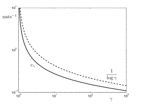
Figure 3: The coefficient $c_{\gamma}$ in (475) (solid line) compared to $\frac{1}{\log\gamma}$ (cf. (472)) (dashed line).

It can be verified that the bound in Theorem 33 is tighter than (472) since $c_{\gamma}<\frac{1}{\log\gamma}$ for $\gamma>1$, and the additional positive summand $\frac{2\log e}{e\log\gamma}$ in the right side of (472) further loosens the bound (472) in comparison to (474). According to the approximation of $c_{\gamma}$ in (496) and (497), we have for large values of $\gamma$

$$c_{\gamma}\approx\frac{1}{\log\left(\frac{\alpha\gamma\log\gamma}{e\log e}\right)}.$$ (498)

Remark 42

The impossibility of a general lower bound on $E_{\gamma}(P\|Q)$, for $\gamma>1$, in terms of the relative entropy $D(P\|Q)$ is evident from Example 13.

Remark 43

The fact that $\{c_{\gamma}\}_{\gamma\geq 1}$ in (475) is monotonically decreasing in $\gamma$ (see Figure 3) is consistent with (474) and the fact that the $E_{\gamma}$ divergence is monotonically decreasing in $\gamma$.

Remark 44

The fact that the behavior of $D(P\|Q)$ for small $|P-Q|$ is quadratic rather than linear does not contradict Theorem 33 because $\lim_{\gamma\downarrow 1}c_{\gamma}=+\infty$ (see Figure 3).

In view of (439) and (474) we obtain

Corollary 4

If $P\ll Q$, $\gamma>1$ and $\mathcal{F}\in\mathscr{F}$, then

$$P(\mathcal{F})\leq\gamma\,Q(\mathcal{F})+c_{\gamma}\,D(P\|Q).$$ (499)

Corollary 5

If $P\ll Q$ and $\gamma>1$, then

$$E_{\gamma}(P\|Q)\leq\min_{\lambda\in[0,1]}\left\{\tfrac{\lambda}{2}\,|P-Q|+c_{\gamma}\,D\bigl{(}(1-\lambda)P+\lambda Q\,\|\,Q\bigr{)}\right\}.$$ (500)

Proof:

For $\lambda\in[0,1]$, let $R=(1-\lambda)P+\lambda Q$. Then, we have for $\gamma>1$,

$$E_{\gamma}(P\|Q) \leq\tfrac{1}{2}\,|P-R|+E_{\gamma}(R\|Q)$$ (501)

$$=\tfrac{\lambda}{2}\,|P-Q|+E_{\gamma}\bigl{(}(1-\lambda)P+\lambda Q\,\|Q\bigr{)}$$ (502)

$$\leq\tfrac{\lambda}{2}\,|P-Q|+c_{\gamma}\,D\bigl{(}(1-\lambda)P+\lambda Q\,\|\,Q\bigr{)}$$ (503)

where (501) is (444); and (503) follows from (474). ∎

Remark 45

Note that the upper bounds in the right sides of (447) and (485) follow from (500) by setting $\lambda=1$ or $\lambda=0$, respectively.

Remark 46

Further upper bounding the right side of (503) by invoking Pinsker’s inequality and the convexity of relative entropy, followed by an optimization over the free parameter $\lambda\in[0,1]$, does not lead to an improvement beyond the minimum of the bounds in (473) and (485).

VII-D Lower Bound on $\mathds{F}_{P\|Q}$ as a Function of $D(P\|Q)$

The $E_{\gamma}$ divergence proves to be instrumental in the proof of the following bound on the complementary relative information spectrum for positive arguments.

Theorem 34

If $P\ll Q$, $P\neq Q$, and $\beta>1$, then

$$\frac{1-\mathds{F}_{P\|Q}(\log\beta)}{D(P\|Q)} \leq u(\beta)\triangleq\min_{\gamma\in(1,\beta)}\left(\frac{\beta\,c_{\gamma}}{\beta-\gamma}\right),$$ (504)

where $c_{\gamma}$ is given in (475). Furthermore, the function $u\colon(1,\infty)\to\mathbb{R}^{+}$ is monotonically decreasing with

$$u(\beta)\leq\frac{2}{\log\left(\frac{\beta}{2e}\right)},\quad\forall\,\beta>2e.$$ (505)

Proof:

For $\beta>1$, denote the event

$$\mathcal{F}_{\beta}\triangleq\left\{x\in\mathcal{A}\colon\imath_{P\|Q}(x)>\log\beta\right\}$$ (506)

which satisfies

$$P(\mathcal{F}_{\beta})>\beta\,Q(\mathcal{F}_{\beta}).$$ (507)

Then,

$$1-\mathds{F}_{P\|Q}(\log\beta) =P(\mathcal{F}_{\beta})$$ (508)

$$\leq\inf_{\gamma\in(1,\beta)}\frac{P(\mathcal{F}_{\beta})-\gamma\,Q(\mathcal{F}_{\beta})}{1-\frac{\gamma}{\beta}}$$ (509)

$$\leq\inf_{\gamma\in(1,\beta)}\frac{\beta\,E_{\gamma}(P\|Q)}{\beta-\gamma}$$ (510)

$$\leq\inf_{\gamma\in(1,\beta)}\left(\frac{\beta\,c_{\gamma}}{\beta-\gamma}\right)\,D(P\|Q)$$ (511)

where (508) holds by Definition 2; (509) follows from (507); (510) is satisfied by (439), and (511) is due to (474). Note that the infimum in (511) is attained because $c_{\gamma}$ is continuous and for $\beta>1$, $\frac{\beta\,c_{\gamma}}{\beta-\gamma}$ tends to $+\infty$ at both extremes of the interval $(1,\beta)$. The monotonicity of $u(\beta)$ and the bound in (505) are proved in Appendix I. ∎

VIII Rényi Divergence

The Rényi divergence (Definition 4) admits a variational representation in terms of the relative entropy [94, Theorem 1]. Let $P_{\mathtt{1}}\ll P_{\mathtt{0}}$ then, for $\alpha>0$,

$$(1-\alpha)\,D_{\alpha}(P_{\mathtt{1}}\|P_{\mathtt{0}})=\min_{P\ll P_{\mathtt{1}}}\bigl{\{}\alpha\,D(P\|P_{\mathtt{1}})+(1-\alpha)\,D(P\|P_{\mathtt{0}})\bigr{\}}.$$ (512)

In this section, integral expressions for the Rényi divergence are derived in terms of the relative information spectrum (Definition 2). These expressions are used to obtain bounds on the Rényi divergence as a function of the variational distance under the assumption of bounded relative information.

VIII-A Expressions in Terms of the Relative Information Spectrum

To state the results in this section, it is convenient to introduce $\zeta_{\alpha}\colon(0,\infty)\to[0,\infty)$

$$\zeta_{\alpha}(\beta)=\beta^{\alpha-2}\;\left(1-\mathds{F}_{P\|Q}\bigl{(}\log\beta\bigr{)}\right).$$ (513)

The Rényi divergence admits the following representation in terms of the relative information spectrum and the relative information bounds $(\beta_{1},\beta_{2})\in[0,1]^{2}$ in (151)–(152).

Theorem 35

Let $P\ll Q$.

• If $\beta_{1}>0$ and $\alpha\in(0,1)\cup(1,\infty)$, then

  $$D_{\alpha}(P\|Q) =\frac{1}{\alpha-1}\;\log\biggl{(}\beta_{1}^{1-\alpha}+(1-\alpha)\int_{\beta_{2}}^{\beta_{1}^{-1}}\bigl{(}\beta^{\alpha-2}-\zeta_{\alpha}(\beta)\bigr{)}\text{d}\beta\biggr{)}.$$ (514)

• If $\beta_{1}=0$ and $\alpha\in(0,1)$, then

  $$D_{\alpha}(P\|Q) =\frac{1}{\alpha-1}\;\log\left((1-\alpha)\displaystyle\int_{\beta_{2}}^{\infty}\bigl{(}\beta^{\alpha-2}-\zeta_{\alpha}(\beta)\bigr{)}\;\text{d}\beta\right).$$ (515)

• If $\alpha\in(1,\infty)$, then

  $$D_{\alpha}(P\|Q) =\frac{1}{\alpha-1}\;\log\left((\alpha-1)\displaystyle\int_{0}^{\infty}\zeta_{\alpha}(\beta)\;\text{d}\beta\right)$$ (516)

  $$=\frac{1}{\alpha-1}\;\log\left(\beta_{2}^{\alpha-1}+(\alpha-1)\displaystyle\int_{\beta_{2}}^{\infty}\zeta_{\alpha}(\beta)\;\text{d}\beta\right).$$ (517)

Proof:

If $\alpha>1$, (78) implies that $D_{\alpha}(P\|Q)$ is given by

$$\frac{1}{\alpha-1}\;\log\Bigl{(}\mathbb{E}\bigl{[}\exp\bigl{(}(\alpha-1)\,\imath_{P\|Q}(X)\bigr{)}\bigr{]}\Bigr{)} =\frac{1}{\alpha-1}\;\log\left(\int_{0}^{\infty}\mathbb{P}\left[\exp\bigl{(}(\alpha-1)\,\imath_{P\|Q}(X)\bigr{)}>t\right]\text{d}t\right)$$ (518)

$$=\frac{1}{\alpha-1}\;\log\left(\int_{0}^{\infty}\mathbb{P}\left[\imath_{P\|Q}(X)>\frac{\log t}{\alpha-1}\right]\,\text{d}t\right)$$ (519)

where (518) follows from (275) for an arbitrary non-negative random variable $V$, and we use $\alpha>1$ to write (519). Then, (516) holds by the definition of the relative information spectrum in (29) and by changing the integration variable $t=\beta^{\alpha-1}$. If $\beta_{1}>0$, the integrand in the right side of (516) is zero in $[\beta_{1}^{-1},\infty)$ and the expression in (514) is readily verified (for $\alpha>1$). More generally (without requiring $\beta_{1}>0$), we split the integral in the right side of (516) into $[0,\beta_{2})\cup[\beta_{2},\infty)$, and (517) follows since the integral over the leftmost interval is $\beta_{2}^{\alpha-1}$ considering that $\mathds{F}_{P\|Q}(\log\beta)=0$ therein.

If $\alpha\in(0,1)$, we write $D_{\alpha}(P\|Q)$ as

$$\frac{1}{\alpha-1}\;\log\Bigl{(}\mathbb{E}\bigl{[}\exp\bigl{(}(\alpha-1)\,\imath_{P\|Q}(X)\bigr{)}\bigr{]}\Bigr{)} =\frac{1}{\alpha-1}\;\log\left(\int_{0}^{\infty}\mathbb{P}\left[\exp\bigl{(}(\alpha-1)\,\imath_{P\|Q}(X)\bigr{)}\geq t\right]\text{d}t\right)$$ (520)

$$=\frac{1}{\alpha-1}\;\log\left(\int_{0}^{\infty}\mathbb{P}\left[\imath_{P\|Q}(X)\leq\frac{\log t}{\alpha-1}\right]\,\text{d}t\right)$$ (521)

$$=\frac{1}{\alpha-1}\;\log\left(\int_{\infty}^{0}\mathbb{P}\left[\imath_{P\|Q}(X)\leq\log\beta\right]\,(\alpha-1)\,\beta^{\alpha-2}\,\text{d}\beta\right)$$

$$=\frac{1}{\alpha-1}\;\log\left((1-\alpha)\int_{\beta_{2}}^{\infty}\beta^{\alpha-2}\;\mathds{F}_{P\|Q}\bigl{(}\log\beta\bigr{)}\;\text{d}\beta\right)$$ (522)

which is the expression in (515). If $\beta_{1}>0$, then we can further split the integral in the right side of (522) into the intervals $[\beta_{2},\beta_{1}^{-1})\cup[\beta_{1}^{-1},\infty)$. Over the rightmost interval, $\mathds{F}_{P\|Q}\bigl{(}\log\beta\bigr{)}=1$ and the integral is seen to be $\beta_{1}^{1-\alpha}$, thereby verifying (514) for $\alpha\in(0,1)$. ∎

The close relationship between the Rényi and Hellinger divergences in (82) results is the following integral representations for the Hellinger divergence.

Corollary 6

Let $P\ll Q$.

• If $\beta_{1}>0$ and $\alpha\in(0,1)\cup(1,\infty)$, then

  $$\mathscr{H}_{\alpha}(P\|Q) =\frac{\beta_{1}^{1-\alpha}-1}{\alpha-1}-\int_{\beta_{2}}^{\beta_{1}^{-1}}\bigl{(}\beta^{\alpha-2}-\zeta_{\alpha}(\beta)\bigr{)}\text{d}\beta.$$ (523)

• If $\beta_{1}=0$ and $\alpha\in(0,1)$, then

  $$\mathscr{H}_{\alpha}(P\|Q) =\frac{1}{1-\alpha}-\int_{\beta_{2}}^{\infty}\bigl{(}\beta^{\alpha-2}-\zeta_{\alpha}(\beta)\bigr{)}\text{d}\beta.$$ (524)

• If $\alpha\in(1,\infty)$, then

  $$\mathscr{H}_{\alpha}(P\|Q) =\int_{0}^{\infty}\zeta_{\alpha}(\beta)\;\text{d}\beta-\frac{1}{\alpha-1}$$ (525)

  $$=\frac{\beta_{2}^{\alpha-1}-1}{\alpha-1}+\displaystyle\int_{\beta_{2}}^{\infty}\zeta_{\alpha}(\beta)\;\text{d}\beta.$$ (526)

Proof:

Combining (82) with (514), (515), (516), (517) yields (523)–(526), respectively. ∎

Particularizing (513), (516) and (525) to $\alpha=2$, we obtain

$$D_{2}(P\|Q) =\log\left(\int_{0}^{\infty}\left(1-\mathds{F}_{P\|Q}(\log\beta)\right)\;\text{d}\beta\right),$$ (527)

$$\chi^{2}(P\|Q) =\int_{0}^{\infty}\left(1-\mathds{F}_{P\|Q}(\log\beta)\right)\,\text{d}\beta-1$$ (528)

$$=\int_{1}^{\infty}\left(1-\mathds{F}_{P\|Q}(\log\beta)\right)\,\text{d}\beta-\int_{0}^{1}\mathds{F}_{P\|Q}(\log\beta)\,\text{d}\beta.$$ (529)

Note the resemblance of the integral expressions in (273) and (529) for $D(P\|Q)$ and $\chi^{2}(P\|Q)$, respectively.

We conclude this subsection by proving three properties of the Hellinger divergence as a function of its order. The first two monotonicity properties are analogous to [37, Theorems 3 and 16] for the Rényi divergence; these monotonicity properties have been originally stated in [65, Proposition 2.7], though the following alternative proof is more transparent.

Theorem 36

The Hellinger divergence satisfies the following properties:

1. $\mathscr{H}_{\alpha}(P\|Q)$ is monotonically increasing in $\alpha\in(0,\infty)$;

2. $\left(\frac{1}{\alpha}-1\right)\mathscr{H}_{\alpha}(P\|Q)$ is monotonically decreasing in $\alpha\in(0,1)$;

3. $\frac{1}{\alpha}\,\mathscr{H}_{\alpha}(P\|Q)$ is log-convex in $\alpha\in(0,\infty)$, which implies that for every $\alpha,\beta>0$

   $$\mathscr{H}^{2}_{\frac{\alpha+\beta}{2}}(P\|Q)\leq\frac{(\alpha+\beta)^{2}}{4\alpha\beta}\;\mathscr{H}_{\alpha}(P\|Q)\,\mathscr{H}_{\beta}(P\|Q).$$ (530)

Proof:

1. From (41) and (54), we have

   $$\mathscr{H}_{\alpha}(P\|Q)=D_{f_{\alpha}}(P\|Q)$$ (531)

   with

   $$f_{\alpha}(t)=\frac{t^{\alpha}-\alpha(t-1)-1}{\alpha-1},\quad t>0,$$ (532)

   whose derivative is

   $$\frac{\partial}{\partial\alpha}\,f_{\alpha}(t)=\frac{t\,r(t^{\alpha-1})}{(\alpha-1)^{2}\,\log e}>0$$ (533)

   where the function $r\colon(0,\infty)\to\mathbb{R}$ is defined in (45). Since it is strictly positive except at $t=1$, $f_{\alpha}$ is monotonically increasing in $\alpha\in(0,\infty)$. Hence, Part a) follows from (531).

2. From (531), for $\alpha\in(0,1)$, we have

   $$\left(\frac{1}{\alpha}-1\right)\,\mathscr{H}_{\alpha}(P\|Q)=D_{g_{\alpha}}(P\|Q)$$ (534)

   where $g_{\alpha}\colon(0,\infty)\to\mathbb{R}$ is the convex function

   $$g_{\alpha}(t) =t-1-\frac{t^{\alpha}-1}{\alpha},\quad t>0.$$ (535)

   with derivative

   $$\frac{\partial}{\partial\alpha}\,g_{\alpha}(t)=-\frac{r(t^{\alpha})}{\alpha^{2}\,\log e}<0,$$ (536)

   so $g_{\alpha}$ is monotonically decreasing in $\alpha\in(0,1)$. Hence, Part b) follows from (534).

3. To prove the log-convexity of $\frac{1}{\alpha}\,\mathscr{H}_{\alpha}(P\|Q)$ in $\alpha\in(0,\infty)$, we rely on [95, Theorem 2.1] which states that if $W$ is a non-negative random variable, then $\lambda_{\alpha}$ in (315) is log-convex in $\alpha$. The claim now follows from (315) by setting $W=\frac{\mathrm{d}P}{\mathrm{d}Q}\,(Y)$ with $Y\sim Q$, which yields that $\lambda_{\alpha}=\frac{1}{\alpha}\,\mathscr{H}_{\alpha}(P\|Q)\log e$ for $\alpha\in(0,\infty)$.

∎

VIII-B Bounds as a Function of the Total Variation Distance

Just as with Pinsker’s inequality, for any $\varepsilon\in(0,2]$, the minimum value of $D_{\alpha}(P\|Q)$ compatible with $|P-Q|\geq\varepsilon$, is achieved with distributions on a binary alphabet [92, Proposition 1]:

$$\min_{P,Q\colon|P-Q|\geq\varepsilon}D_{\alpha}(P\|Q)=\min_{p,q\colon|p-q|\geq\frac{\varepsilon}{2}}d_{\alpha}(p\|q)$$ (537)

where the binary order-$\alpha$ Rényi divergence is defined as

$$d_{\alpha}(p\|q)\triangleq\left\{\begin{array}[]{ll}\frac{1}{\alpha-1}\log\Bigl{(}p^{\alpha}q^{1-\alpha}+(1-p)^{\alpha}(1-q)^{1-\alpha}\Bigr{)},&\mbox{if $\alpha\neq 1$}\\[5.69046pt] p\,\log\frac{p}{q}+(1-p)\,\log\frac{1-p}{1-q},&\mbox{if $\alpha=1$.}\end{array}\right.$$ (540)

We proceed to use Theorem 35 to get an upper bound on $D_{\alpha}(P\|Q)$ expressed in terms of $|P-Q|$.

Theorem 37

If $\beta_{1}\in(0,1)$ and $\alpha\in(0,1)\cup(1,\infty)$, then

$$D_{\alpha}(P\|Q)\leq\frac{1}{\alpha-1}\;\log\left(1+\frac{|P-Q|}{2}\,\frac{\beta_{1}^{1-\alpha}-1}{1-\beta_{1}}\right).$$ (541)

Proof:

Regardless of whether $\alpha<1$ or $\alpha>1$, we can only get an upper bound if, in view of (513), in the integral in (514) we drop the interval $[\beta_{2},1]$:

$$D_{\alpha}(P\|Q) \leq\frac{1}{\alpha-1}\;\log\left(\beta_{1}^{1-\alpha}+(1-\alpha)\int_{1}^{\beta_{1}^{-1}}\beta^{\alpha-2}\;\mathds{F}_{P\|Q}(\log\beta)\;\text{d}\beta\right)$$

$$=\frac{1}{\alpha-1}\;\log\left(1-(1-\alpha)\int_{1}^{\beta_{1}^{-1}}\beta^{\alpha-2}\;\bigl{(}1-\mathds{F}_{P\|Q}(\log\beta)\bigr{)}\;\text{d}\beta\right)$$

$$=\frac{1}{\alpha-1}\;\log\Bigl{(}1+(\alpha-1)\delta\,\mathbb{E}[W^{\alpha}]\Bigr{)}$$ (542)

where (542) holds with $\delta=\tfrac{1}{2}|P-Q|$ and $W\sim p_{1}$ where $p_{1}$ is the probability density function supported on $[1,\beta_{1}^{-1}]$:

$$p_{1}(\beta)=\frac{1}{\delta\beta^{2}}\left(1-\mathds{F}_{P\|Q}(\log\beta)\right).$$ (543)

Note that $p_{1}$ is indeed a probability density function due to (268). In order to proceed, we derive an upper bound on $\mathbb{E}[W^{\alpha}]$ expressed in terms of $|P-Q|$ by invoking Lemma 5 in Appendix J. To that end, denote the monotonically increasing and non-negative function $g(x)=x^{\alpha}$ for $x\geq 0$, and let $p_{2}$ be the probability density function supported on $[1,\beta_{1}^{-1}]$:

$$p_{2}(\beta)=\frac{1}{1-\beta_{1}}\,\frac{1}{\beta^{2}}.$$ (544)

Note that, on their support, $\beta^{2}p_{1}(\beta)$ is monotonically decreasing while $\beta^{2}p_{2}(\beta)$ is constant. Therefore, we can apply Lemma 5 to $W\sim p_{1}$ and $V\sim p_{2}$ to obtain

$$\mathbb{E}\bigl{[}W^{\alpha}\bigr{]} \leq\mathbb{E}\bigl{[}V^{\alpha}\bigr{]}=\frac{\beta_{1}^{1-\alpha}-1}{(1-\beta_{1})(\alpha-1)}.$$ (545)

which gives the desired result upon substituting in (542). ∎

Corollary 7

If $\beta_{1}\in(0,1)$ and $\alpha\in(0,1)\cup(1,\infty)$, then

$$\mathscr{H}_{\alpha}(P\|Q)\leq\frac{\beta_{1}^{1-\alpha}-1}{2(\alpha-1)(1-\beta_{1})}\cdot|P-Q|.$$ (546)

Proof:

Combining (82) and (541) yields (546). ∎

Particularizing (546) to $\alpha=2$ yields

$$\chi^{2}(P\|Q)\leq\tfrac{1}{2}\,\beta_{1}^{-1}\,|P-Q|$$ (547)

which improves the bound in (173) if either $\beta_{1}\leq\tfrac{1}{2}$ or $\beta_{2}=0$.

The combination of (1), (4) and (547) yields the following bound:

Corollary 8

If $\beta_{1}>0$, then

$$\chi^{2}(P\|Q)\leq\frac{1}{\beta_{1}}\sqrt{\min\left\{\frac{D(P\|Q)}{2\log e},\,1-\exp\bigl{(}-D(P\|Q)\bigr{)}\right\}}.$$ (548)

Example 14

Let $P$, $Q$ be defined on $\mathcal{A}=\{0,1\}$ with $P(0)=Q(1)=\tfrac{1}{100}$, which implies that $\beta_{1}=\tfrac{1}{99}$. Then $\chi^{2}(P\|Q)=97.01$, and the bound in (548) is equal to 98.45 in contrast to the upper bound in (188) whose value is 121.17.

Remark 47

By letting $\alpha\to\infty$ in (541), we obtain $D_{\infty}(P\|Q)\leq\log\frac{1}{\beta_{1}}$, which shows that the bound in (541) is asymptotically tight (cf. (81)).

Remark 48

By letting $\alpha\to 1$ in (541), we get (369). Therefore, Theorem 37 generalizes [109, Theorem 7].

Remark 49

By letting $\alpha\to 0$, it follows from (541) that

$$D_{0}(P\|Q)\leq\log\left(\frac{1}{1-\tfrac{1}{2}|P-Q|}\right),$$ (549)

a bound which, in view of (79), is achieved with equality in the case of a finite alphabet with

$$P(a)=\left\{\begin{array}[]{ll}\frac{Q(a)}{1-\delta},&a\in\mathcal{F}\\ 0,&a\in\mathcal{F}^{c}\end{array}\right.$$ (552)

with the event $\mathcal{F}$ selected to satisfy $Q(\mathcal{F})=1-\delta$.

Remark 50

Another upper bound on the Rényi divergence can be obtained by the simpler bound

$$\mathbb{E}[W^{\alpha}]\leq\beta_{1}^{-\alpha},$$ (553)

which holds because $W\in[1,\beta_{1}^{-1}]$. Combining (542) and (553) yields

$$D_{\alpha}(P\|Q)\leq\frac{1}{\alpha-1}\;\log\bigl{(}1+(\alpha-1)\delta\beta_{1}^{-\alpha}\bigr{)}.$$ (554)

Note that, in the limit $\alpha\to 0$, the bounds in (541) and (554) coincide and are equal to the tight bound $-\log(1-\delta)$.

Remark 51

Alternatively, we have the bound

$$D_{\alpha}(P\|Q)\leq\frac{1}{\alpha-1}\,\log\left((1-\delta)^{1-\alpha}+\delta(\alpha-1)\int_{\frac{1}{1-\delta}}^{\frac{1}{\beta_{1}}}\frac{\beta^{\alpha-1}}{\beta-1}\,\text{d}\beta\right)$$ (555)

obtained from (542) and

$$\mathbb{E}[W^{\alpha}] \leq\frac{(1-\delta)^{1-\alpha}-1}{\delta(\alpha-1)}+\int_{\frac{1}{1-\delta}}^{\frac{1}{\beta_{1}}}\frac{\beta^{\alpha-1}}{\beta-1}\,\text{d}\beta.$$ (556)

which holds since, in view of (543) and (290),

$$p_{1}(\beta)\leq\left\{\begin{array}[]{ll}\frac{1}{\delta\beta^{2}},&\beta\in\bigl{[}0,\,\frac{1}{1-\delta}\bigr{]}\\[5.69046pt] \frac{1}{\beta(\beta-1)},&\beta\in\bigl{[}\frac{1}{1-\delta},\,\beta_{1}^{-1}\bigr{]}\\[5.69046pt] 0&\mbox{otherwise.}\end{array}\right.$$ (560)

The upper bounds in (541) and (555) asymptotically coincide in the limit where $\alpha\to\infty$, giving the common limit of $\log\left(\frac{1}{\beta_{1}}\right)$ which is a tight upper bound (cf. Remark 47).

VIII-C Bounds as a Function of the Relative Entropy

In this section, we provide upper and lower bounds on the Rényi divergence $D_{\alpha}(P\|Q)$, for an arbitrary order $\alpha\in(0,1)\cup(1,\infty)$, expressed in terms of the relative entropy $D(P\|Q)$ and $\beta_{1},\beta_{2}$.

Theorem 38

Let $(\beta_{1},\beta_{2})\in[0,1)^{2}$, $\alpha\in(0,1)\cup(1,\infty)$, and $u_{\alpha}\colon[0,\infty]\to[0,\infty]$ be

$$u_{\alpha}=\frac{\alpha-1}{\kappa_{\alpha}(t)}$$ (561)

with $\kappa_{\alpha}$ defined in (183).

1. If $\alpha\in(0,1)$, then

   $$\frac{1}{\alpha-1}\,\log\Bigl{(}1+u_{\alpha}(\beta_{1}^{-1})\,D(P\|Q)\Bigr{)}$$

   $$\leq D_{\alpha}(P\|Q)$$ (562)

   $$\leq\min\left\{D(P\|Q),\;\frac{1}{\alpha-1}\,\log\Bigl{(}1+u_{\alpha}(\beta_{2})\,D(P\|Q)\Bigr{)}^{+}\right\}.$$ (563)

2. If $\alpha\in(1,\infty)$, then

   $$\max\left\{D(P\|Q),\;\frac{1}{\alpha-1}\,\log\Bigl{(}1+u_{\alpha}(\beta_{2})\,D(P\|Q)\Bigr{)}\right\}$$

   $$\leq D_{\alpha}(P\|Q)$$ (564)

   $$\leq\min\left\{\log\frac{1}{\beta_{1}},\;\frac{1}{\alpha-1}\,\log\Bigl{(}1+u_{\alpha}(\beta_{1}^{-1})\,D(P\|Q)\Bigr{)}\right\}.$$ (565)

3. Furthermore, if $\alpha\in(0,1)\cup(1,\infty)$, then

   $$D_{\alpha}(P\|Q)\leq\frac{1}{\alpha-1}\,\log\left(1+\frac{\mkern 1.5mu\overline{\mkern-1.5mu\delta\mkern-1.5mu}\mkern 1.5mu\,(\beta_{1}^{1-\alpha}-1)}{1-\beta_{1}}\right)$$ (566)

   where

   $$\mkern 1.5mu\overline{\mkern-1.5mu\delta\mkern-1.5mu}\mkern 1.5mu^{2}=\min\left\{\frac{D(P\|Q)}{2\log e},\,1-\exp\bigl{(}-D(P\|Q)\bigr{)}\right\}.$$ (567)

Proof:

Parts a) and b) follow from Theorem 9 in view of (82), from the fact that $D_{\alpha}(P\|Q)$ is monotonically increasing in $\alpha>0$, and from $D_{\infty}(P\|Q)=\log\frac{1}{\beta_{1}}$.

Part c) follows from Theorem 37 replacing $\delta\triangleq\tfrac{1}{2}\,|P-Q|$ by its upper bound $\mkern 1.5mu\overline{\mkern-1.5mu\delta\mkern-1.5mu}\mkern 1.5mu$ obtained from (1) and (4). ∎

The next three remarks address the tightness of the bounds (562)–(563) and (564)–(565).

Remark 52

The constants $u_{\alpha}(\beta_{1}^{-1})$ and $u_{\alpha}(\beta_{2})$ in (562)–(563) and (564)–(565) are the best possible among all probability measures $P,Q$ with given $(\beta_{1},\beta_{2})\in[0,1)^{2}$. This follows from (82), and in view of the tightness of the constants in Theorem 9 (Remark 11).

Remark 53

Let $P$, $Q=Q_{\varepsilon}$ be defined on a binary alphabet with $P(0)=\tfrac{1}{2}$ and $Q(0)=\tfrac{1}{2}-\varepsilon$. Then, it is easy to verify that the ratio of the upper to lower bounds in Parts a) and b) converges to 1 as $\varepsilon\to 0$.

Remark 54

Let $P$ and $Q$ be defined on a binary alphabet with $P(0)=\tfrac{1}{2}$, $Q(0)=\varepsilon\in(0,1)$. Then, in the limit $\varepsilon\to 0$, the ratio of $D_{\alpha}(P\|Q)$ to the left side of (562) is equal to $\frac{\alpha}{\log_{2}\left(\frac{2}{2-\alpha}\right)}\in(1,\log_{e}(4))$ for $\alpha\in(0,1)$. Moreover, if $\varepsilon\to 0$, the ratio of $D_{\alpha}(P\|Q)$ and the right side of (565) tends to 1 for $\alpha\in(1,\infty)$.

To prove the first part of Remark 54, in view of (562), one needs to show that for $\alpha\in(0,1)$

$$\lim_{\varepsilon\downarrow 0}\frac{(\alpha-1)\,d_{\alpha}(\tfrac{1}{2}\|\varepsilon)}{\log\Bigl{(}1+u_{\alpha}\bigl{(}\frac{1}{2\varepsilon}\bigr{)}\,d(\tfrac{1}{2}\|\varepsilon)\Bigr{)}}=\frac{\alpha}{\log_{2}\left(\frac{2}{2-\alpha}\right)}$$ (568)

where $d(\cdot\|\cdot)\triangleq d_{1}(\cdot\|\cdot)$ and $d_{\alpha}(\cdot\|\cdot)$ are given in (540). This can be verified by using (540) and (561) to show that if $\alpha\in(0,1)$, then in the limit $\varepsilon\to 0$

$$d\bigl{(}\tfrac{1}{2}\|\varepsilon\bigr{)}=\tfrac{1}{2}\,\bigl{(}1+o(1)\bigr{)}\,\log\left(\tfrac{1}{2\varepsilon}\right),$$ (569)

$$(\alpha-1)\,d_{\alpha}\bigl{(}\tfrac{1}{2}\|\varepsilon\bigr{)}=-\alpha\bigl{(}1+o(1)\bigr{)}\,\log 2,$$ (570)

$$u_{\alpha}\bigl{(}\tfrac{1}{2\varepsilon}\bigr{)}=-\frac{\alpha\bigl{(}1+o(1)\bigr{)}}{\log\bigl{(}\frac{1}{2\varepsilon}\bigr{)}}.$$ (571)

Assembling (569)–(571) yields (568) whose right side is monotonically decreasing in $\alpha\in(0,1)$, and bounded between 1 (by letting $\alpha\to 1$) and $\log_{e}(4)$ (by letting $\alpha\to 0$).

To prove the second part of Remark 54, in view of (565), one needs to show that for $\alpha\in(1,\infty)$

$$\lim_{\varepsilon\downarrow 0}\frac{(\alpha-1)\,d_{\alpha}(\tfrac{1}{2}\|\varepsilon)}{\log\Bigl{(}1+u_{\alpha}\bigl{(}\frac{1}{2\varepsilon}\bigr{)}\,d(\tfrac{1}{2}\|\varepsilon)\Bigr{)}}=1.$$ (572)

From (540) and (561), it follows that in the limit where $\varepsilon$ tends to zero

$$(\alpha-1)\,d_{\alpha}\bigl{(}\tfrac{1}{2}\|\varepsilon\bigr{)}=\log\left(2^{-\alpha}\,\varepsilon^{1-\alpha}\right)\,\bigl{(}1+o(1)\bigr{)},$$ (573)

$$u_{\alpha}\bigl{(}\tfrac{1}{2\varepsilon}\bigr{)}=\frac{1+o(1)}{(2\varepsilon)^{\alpha-1}\,\log\bigl{(}\frac{1}{2\varepsilon}\bigr{)}}.$$ (574)

Assembling (569), (573) and (574) yields (572) for $\alpha\in(1,\infty)$.

Example 15

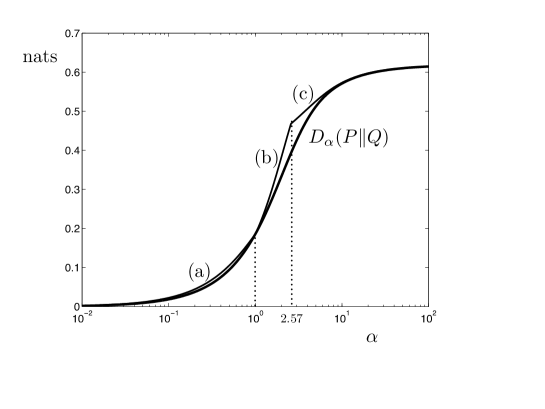
Figure 4: The Rényi divergence $D_{\alpha}(P\|Q)$ for $\mathcal{A}=\{0,1\}$ with $P(0)=Q(1)=0.65$, compared to the tightest upper bound in Theorem 38: (a) (563) for $\alpha\in(0,1)$; (b): (565) for $\alpha\in[1,2.57]$; (c): (566) for $\alpha>2.57$.

Figure 4 illustrates the upper bounds on $D_{\alpha}(P\|Q)$ in Theorem 38 for binary alphabets.

Remark 55

[40, Proposition 11] shows an upper bound on $D_{\alpha}(P\|Q)$ for $\alpha\in[1,\tfrac{5}{4}]$, which is expressed in terms of $D(P\|Q)$ and the finite cardinalities of the alphabets over which $P$ and $Q$ are defined. Although the bound in [40, (9)] is not tight, it leads to a strong converse for a certain class of discrete memoryless networks.

IX Summary

Since many distance measures of interest fall under the common paradigm of an $f$-divergence, it is not surprising that bounds on the ratios of various $f$-divergences are useful in many instances such as proving convergence of probability measures according to various metrics, analysis of rates of convergence and concentration of measure bounds [13, 41, 76, 82, 89, 111], hypothesis testing [31], testing goodness of fit [50, 85], minimax risk in estimation and modeling [47, 51, 86, 107], strong data processing inequality constants and maximal correlation [1, 81, 84], transportation-cost inequalities [13, 74, 82, 83], contiguity [64, 65], etc.

While the derivation of $f$-divergence inequalities has received considerable attention in the literature, the proof techniques have been tailored to the specific instances. In contrast, we have proposed several systematic approaches to the derivation of $f$-divergence inequalities. Introduced in Section III-A, functional domination emerges as a basic tool to obtain $f$-divergence inequalities. Another basic tool that capitalizes on many cases of interest (including the finite alphabet one) is introduced in Section IV-B, where not only one of the distributions is absolutely continuous with respect to the other but their relative information is almost surely bounded.

Section V-D illustrates the use of moment inequalities and the log-convexity property, while the utility of Lipschitz constraints in deriving bounds is highlighted in Section VI-B.

In addition, new $f$-divergence inequalities (frequently with optimal constants) arise from:

• integral representation of $f$-divergences, expressed in terms of the $E_{\gamma}$ divergence (Section VII-B);

• extension of Pinsker’s inequality to $E_{\gamma}$ divergence (Section VII-C);

• a relation between the relative information and the relative entropy (Section VII-D);

• exact expressions of Rényi divergence in terms of the relative information spectrum (Section VIII-A);

• the exact locus of the entropy and the variational distance from the equiprobable probability mass function (Section VI-D).

Appendix A Completion of the Proof of Theorem 7

Lemma 2

The function $\kappa\colon(0,\infty)\to(0,\infty)$ which is the continuous extension of the function in (174) with $\kappa(1)=1$ is strictly monotonically increasing.

Proof:

From (174) and (176),

$$\kappa^{\prime}(t)=\frac{(t-1)^{2}\log^{2}e-t\log^{2}t}{t\,g^{2}(t)},$$ (575)

if $t\in(0,1)\cup(1,\infty)$, while $\kappa^{\prime}(1)=\tfrac{1}{3}$. To show

$$(t-1)^{2}\,\log^{2}e-t\log^{2}t>0,\quad\forall\,t\in(0,1)\cup(1,\infty).$$ (576)

we substitute $t=\exp(x)$ to obtain that if $x\neq 0$, then

$$s(x)=\exp(2x)-(2+x^{2})\exp(x)+1>0,\;$$ (577)

which holds since $s(0)=0$ and the derivative

$$s^{\prime}(x)=2\exp(x)\left[\exp(x)-\left(1+x+\frac{x^{2}}{2}\right)\right]$$ (578)

is negative on $(-\infty,0)$ and positive on $(0,\infty)$. ∎

Appendix B Proof of the Monotonicity of $\kappa_{\alpha}$ in (183)

To show that the function $\kappa_{\alpha}\colon[0,\infty]\to[0,\infty]$ in (183) is monotonically increasing on $[0,\infty]$ if $\alpha\in(0,1)$ and monotonically decreasing on $[0,\infty]$ if $\alpha\in(1,\infty)$ it is sufficient to show that

$$\frac{\text{d}}{\text{d}t}\left(\frac{r(t)}{1-t^{\alpha}+\alpha(t-1)}\right)>0$$ (579)

for $(\alpha,t)\in\mathcal{F}=((0,1)\cup(1,\infty))^{2}$. From (45), straightforward calculus gives

$$\left[1-t^{\alpha}+\alpha(t-1)\right]^{2}\;\frac{\text{d}}{\text{d}t}\left(\frac{r(t)}{1-t^{\alpha}+\alpha(t-1)}\right)$$ (580)

$$=(1-\alpha)(1-t^{\alpha})\log t-\alpha(1-t)(1-t^{\alpha-1})\log e$$ (581)

$$\triangleq g_{\alpha}(t)$$ (582)

so the desired result will follow upon showing

$$g_{\alpha}(t)>0,\quad(\alpha,t)\in\mathcal{F}.$$ (583)

Note that $g_{\alpha}(1)=0$. For $(\alpha,t)\in\mathcal{F}$, it is easy to verify that

$$(1-\alpha)(t-1)(1-t^{\alpha-1})>0.$$ (584)

A division of (583) by the positive left side of (584) gives the following equivalent inequality:

$$\phi_{\alpha}(t)>\frac{\alpha}{\alpha-1},\quad\forall\,(\alpha,t)\in\mathcal{F}$$ (585)

where, for $\alpha\in(0,1)\cup(1,\infty)$,

$$\phi_{\alpha}(t)\triangleq\left\{\begin{array}[]{ll}\frac{(1-t^{\alpha})\log_{e}t}{(t-1)(1-t^{\alpha-1})}&\mbox{if $t\in(0,1)\cup(1,\infty)$}\\ \frac{\alpha}{\alpha-1}&\mbox{if $t=1$.}\end{array}\right.$$ (588)

We aim to prove (585). Note that, for $\alpha\in(0,1)\cup(1,\infty)$,

$$\lim_{t\to 1}\phi_{\alpha}(t)=\frac{\alpha}{\alpha-1}=\phi_{\alpha}(1)$$ (589)

so, (585) is implied by proving that $\phi_{\alpha}\colon(0,\infty)\to\mathbb{R}$ is monotonically decreasing on $(0,1)$, and it is monotonically increasing on $(1,\infty)$. For this purpose, we rely on the following lemmas.

Lemma 3

For every $t>0$ and $\alpha\in(0,1)\cup(1,\infty)$

$$\phi_{\alpha}(t)=\psi(t)-\left(\frac{1}{1-\alpha}\right)\,\psi(t^{1-\alpha})$$ (590)

where

$$\psi(t)\triangleq\left\{\begin{array}[]{ll}\frac{\log_{e}t}{t-1}&\mbox{if $t\in(0,1)\cup(1,\infty)$}\\ 1&\mbox{if $t=1$.}\end{array}\right.$$ (593)

Proof:

For $\alpha,t\in(0,1)\cup(1,\infty)$

$$\psi(t)-\left(\frac{1}{1-\alpha}\right)\,\psi(t^{1-\alpha}) =\frac{(t^{1-\alpha}-t)\,\log_{e}t}{(t-1)(t^{1-\alpha}-1)}$$ (594)

$$=\frac{(1-t^{\alpha})\,\log_{e}t}{(t-1)(1-t^{\alpha-1})}$$ (595)

$$=\phi_{\alpha}(t)$$ (596)

where (594) holds due to (593), (595) is justified by multiplying the numerator and denominator of (594) by $t^{\alpha-1}$, and (596) is due to (588). Note that (590) is also satisfied at $t=1$ due to the continuity of $\phi_{\alpha}$ and $\psi$ at this point. ∎

Lemma 4

The following inequality holds for $z>0$:

$$\psi^{\prime}(z)+z\psi^{\prime\prime}(z)>0,$$ (597)

Proof:

From the power series expansion of $\log_{e}z$ around $z=1$, we get for $0<z\leq 2$

$$\frac{\log_{e}z}{z-1}=1-\tfrac{1}{2}(z-1)+\tfrac{1}{3}(z-1)^{2}-\tfrac{1}{4}(z-1)^{3}+\ldots$$ (598)

From (593) and (598), $\psi^{\prime}(1)=-\tfrac{1}{2}$ and $\psi^{\prime\prime}(1)=\frac{2}{3}$; at $z=1$, the left side of (597) is equal to

$$\psi^{\prime}(1)+\psi^{\prime\prime}(1)=\tfrac{1}{6}>0.$$ (599)

For $z\in(0,1)\cup(1,\infty)$, the left side of (597) satisfies

$$\psi^{\prime}(z)+z\psi^{\prime\prime}(z)=\frac{m(z)}{z(z-1)^{3}}$$ (600)

where

$$m(z)\triangleq(z+1)\log_{e}z-2(z-1),\quad\forall\,z>0.$$ (601)

From (601)

$$m(1)=0,$$ (602)

$$m^{\prime}(z)=\frac{1}{z}-1-\log_{e}\left(\frac{1}{z}\right)>0,\quad\forall\,z\in(0,1)\cup(1,\infty)$$ (603)

which implies that $m\colon(0,\infty)\to\mathbb{R}$ is monotonically increasing, positive for $z>1$ and negative for $z<1$. These facts together with (599) and (600) yield that (597) holds for all $z>0$. ∎

We proceed now with the proof of (585). For $\alpha\in(0,1)\cup(1,\infty)$, we have

$$\frac{\partial}{\partial\alpha}\phi^{\prime}_{\alpha}(t) =\frac{\partial^{2}}{\partial\alpha\;\partial t}\left[\psi(t)-\left(\frac{1}{1-\alpha}\right)\,\psi(t^{1-\alpha})\right]$$ (604)

$$=\frac{\partial}{\partial\alpha}\Bigl{(}\psi^{\prime}(t)-t^{-\alpha}\,\psi^{\prime}(t^{1-\alpha})\Bigr{)}$$ (605)

$$=-\frac{\partial}{\partial\alpha}\Bigl{(}t^{-\alpha}\,\psi^{\prime}(t^{1-\alpha})\Bigr{)}$$ (606)

$$=t^{-\alpha}\;\log_{e}(t)\;\psi^{\prime}(t^{1-\alpha})-t^{-\alpha}\;\frac{\partial}{\partial\alpha}\psi^{\prime}(t^{1-\alpha})$$ (607)

$$=t^{-\alpha}\;\log_{e}(t)\Bigl{[}\psi^{\prime}(t^{1-\alpha})+t^{1-\alpha}\;\psi^{\prime\prime}(t^{1-\alpha})\Bigr{]}$$ (608)

where (604) follows from (590). From Lemma 4, for $t>0$,

$$\psi^{\prime}(t^{1-\alpha})+t^{1-\alpha}\;\psi^{\prime\prime}(t^{1-\alpha})>0.$$ (609)

From (608) and (609), for $\alpha\in(0,1)\cup(1,\infty)$, and $t\in(0,1)$

$$\frac{\partial}{\partial\alpha}\phi^{\prime}_{\alpha}(t)<0,$$ (610)

and for $t\in(1,\infty)$,

$$\frac{\partial}{\partial\alpha}\phi^{\prime}_{\alpha}(t)>0.$$ (611)

From (590) and the continuity of $\psi^{\prime}$ on $(0,\infty)$ (see (593) and (598)), for all $t>0$,

$$\lim_{\alpha\downarrow 0}\phi^{\prime}_{\alpha}(t) =\lim_{\alpha\downarrow 0}\bigl{(}\psi^{\prime}(t)-t^{-\alpha}\,\psi^{\prime}(t^{1-\alpha})\bigr{)}=0.$$ (612)

Combining (610) and (612) gives that, for $\alpha\in(0,1)$ and $t\in(0,1)$

$$\phi^{\prime}_{\alpha}(t)<0,$$ (613)

and, combining (611) and (612) gives that, for $\alpha\in(0,1)$ and $t\in(1,\infty)$,

$$\phi^{\prime}_{\alpha}(t)>0.$$ (614)

Hence, for $\alpha\in(0,1)$, $\phi_{\alpha}\colon(0,\infty)\to\mathbb{R}$ is monotonically decreasing on $(0,1)$, and it is monotonically increasing on $(1,\infty)$.

We now consider the case where $\alpha\in(1,\infty)$. Since, from (590) and (598),

$$\lim_{\alpha\to 1}\phi^{\prime}_{\alpha}(t) =\lim_{\alpha\to 1}\bigl{(}\psi^{\prime}(t)-t^{-\alpha}\,\psi^{\prime}(t^{1-\alpha})\bigr{)}$$ (615)

$$=\psi^{\prime}(t)+\frac{\psi^{\prime}(1)}{t}$$ (616)

$$=\psi^{\prime}(t)+\frac{1}{2t}$$ (617)

then, the existence of this limit in (615) yields that its one-sided limits are equal, i.e.,

$$\lim_{\alpha\downarrow 1}\phi^{\prime}_{\alpha}(t)=\lim_{\alpha\uparrow 1}\phi^{\prime}_{\alpha}(t).$$ (618)

Consequently, (613), (614) and (618) yield that

$$\begin{split}&\lim_{\alpha\downarrow 1}\phi^{\prime}_{\alpha}(t)\geq 0,\quad\forall\,t\in(0,1),\\ &\lim_{\alpha\downarrow 1}\phi^{\prime}_{\alpha}(t)\leq 0,\quad\forall\,t\in(1,\infty)\end{split}$$ (619)

and, from (610), (611) and (LABEL:eq:phi104), we conclude that (613) and (614) also hold for $\alpha\in(1,\infty)$. The property that $\phi_{\alpha}\colon(0,\infty)\to\mathbb{R}$ is monotonically decreasing on $(0,1)$ and monotonically increasing on $(1,\infty)$ is therefore extended also to $\alpha\in(1,\infty)$. As explained after (589), this implies the satisfiability of (585). Consequently, also (583) holds, which implies that $\kappa_{\alpha}\colon[0,\infty]\to[0,\infty]$, defined in (183), is monotonically increasing for all $\alpha\in(0,1)$, and it is monotonically decreasing for all $\alpha\in(1,\infty)$.

Appendix C Proof of (231)

To verify that (231) follows from (223), fix arbitrarily small $\varepsilon>0$ and $\rho>0$. Consider the partition $\mathcal{A}=\mathcal{A}_{1}^{(n)}\cup\mathcal{A}_{2}^{(n)}\cup\mathcal{A}_{3}^{(n)}$ with

$$\mathcal{A}_{1}^{(n)}\triangleq\left\{a\in\mathcal{A}\colon\frac{\text{d}P_{n}}{\text{d}Q}\,(a)\in[0,1-\rho]\right\},$$ (620)

$$\mathcal{A}_{2}^{(n)}\triangleq\left\{a\in\mathcal{A}\colon\frac{\text{d}P_{n}}{\text{d}Q}\,(a)\in(1-\rho,1+\varepsilon]\right\},$$ (621)

$$\mathcal{A}_{3}^{(n)}\triangleq\left\{a\in\mathcal{A}\colon\frac{\text{d}P_{n}}{\text{d}Q}\,(a)\in(1+\varepsilon,\infty)\right\},$$ (622)

then

$$I_{1}^{(n)}+I_{2}^{(n)}+I_{3}^{(n)}=1$$ (623)

where

$$I_{j}^{(n)}\triangleq\int_{\mathcal{A}_{j}^{(n)}}\frac{\text{d}P_{n}}{\text{d}Q}\,(a)\;\text{d}Q(a).$$ (624)

From the assumption in (223), $I_{3}^{(n)}\to 0$ when $n\to\infty$ since for all sufficiently large $n$

$$Q(\mathcal{A}_{3}^{(n)})=0.$$ (625)

Let

$$d_{n}\triangleq Q(\mathcal{A}_{1}^{(n)})$$ (626)

then, from (625), for all sufficiently large $n$

$$1-d_{n}=Q(\mathcal{A}_{2}^{(n)}).$$ (627)

Consequently, from (620), (621), (623), (625), (626) and (627), it follows that for all sufficiently large $n$,

$$1 =I_{1}^{(n)}+I_{2}^{(n)}$$ (628)

$$\leq d_{n}(1-\rho)+(1-d_{n})(1+\varepsilon)\triangleq\mu_{n}.$$ (629)

If $\liminf d_{n}=0$ for an arbitrarily small $\rho>0$ then (231) holds by the definition in (626). Assuming otherwise, namely,

$$\liminf d_{n}=\theta\in(0,1)$$ (630)

leads to the following contradiction:

$$1 \leq\liminf\mu_{n}$$ (631)

$$\leq(1-\rho)\,\liminf d_{n}+(1+\varepsilon)\,\limsup\,(1-d_{n})$$ (632)

$$=\theta(1-\rho)+(1-\theta)(1+\varepsilon)$$ (633)

$$=1-\frac{\theta\rho}{2}$$ (634)

where $\varepsilon=\frac{\theta\rho}{2(1-\theta)}$; (631) follows from (628), (629); (632) holds by (629); (633) is due to (630).

Appendix D Proof of Theorem 15

Eq. (260) follows from the definitions in (28) and (59). Since $z^{+}=\tfrac{1}{2}\bigl{(}|z|+z\bigr{)}$ and $z^{-}=\tfrac{1}{2}\bigl{(}|z|-z\bigr{)}$, for all $z\in\mathbb{R}$, (261) and (262) follow from (260) and

$$\mathbb{E}\bigl{[}1-\exp(\imath_{P\|Q}(Y))\bigr{]}=\int\left(1-\frac{\mathrm{d}P}{\mathrm{d}Q}\right)\,\mathrm{d}Q=0.$$ (635)

By change of measure, for every measurable function $f\colon\mathcal{A}\to\mathbb{R}$ with $\mathbb{E}\bigl{[}f(X)\bigr{]}<\infty$ and $\mathbb{E}\bigl{[}f(Y)\bigr{]}<\infty$,

$$\mathbb{E}\bigl{[}f(X)\bigr{]} =\mathbb{E}\Bigl{[}\frac{\text{d}P}{\text{d}Q}(Y)\,f(Y)\Bigr{]}=\mathbb{E}\bigl{[}\exp\bigl{(}\imath_{P\|Q}(Y)\bigr{)}\,f(Y)\bigr{]}.$$ (636)

Hence, it follows from (636) that

$$\mathbb{P}\bigl{[}\imath_{P\|Q}(X)>0\bigr{]}=\mathbb{E}\bigl{[}1\bigl{\{}\imath_{P\|Q}(X)>0\bigr{\}}\bigr{]}$$ (637)

$$\hskip 64.01869pt=\mathbb{E}\bigl{[}\exp(\imath_{P\|Q}(Y))1\bigl{\{}\imath_{P\|Q}(Y)>0\bigr{\}}\bigr{]}$$ (638)

and

$$\mathbb{P}\bigl{[}\imath_{P\|Q}(X)\leq 0\bigr{]}=\mathbb{E}\bigl{[}1\bigl{\{}\imath_{P\|Q}(X)\leq 0\bigr{\}}\bigr{]}$$ (639)

$$\hskip 62.88077pt=\mathbb{E}\bigl{[}\exp(\imath_{P\|Q}(Y))1\bigl{\{}\imath_{P\|Q}(Y)\leq 0\bigr{\}}\bigr{]}.$$ (640)

To show (263), note that from (262) and the change of measure in (636), we get

$$\tfrac{1}{2}\,|P-Q| =\mathbb{E}\bigl{[}\bigl{(}1-\exp(\imath_{P\|Q}(Y))\bigr{)}^{-}\bigr{]}$$ (641)

$$=\mathbb{E}\bigl{[}\bigl{(}\exp(\imath_{P\|Q}(Y))-1\bigr{)}\;1\bigl{\{}\imath_{P\|Q}(Y)>0\bigr{\}}\bigr{]}$$ (642)

$$=\mathbb{E}\bigl{[}\bigl{(}1-\exp(-\imath_{P\|Q}(X))\bigr{)}\;1\bigl{\{}\imath_{P\|Q}(X)>0\bigr{\}}\bigr{]}$$ (643)

$$=\mathbb{E}\bigl{[}\bigl{(}1-\exp(-\imath_{P\|Q}(X))\bigr{)}^{+}\bigr{]}.$$ (644)

To show (264) and (265), we get from (262) and (638)

$$\tfrac{1}{2}\,|P-Q| =\mathbb{E}\bigl{[}\bigl{(}1-\exp(\imath_{P\|Q}(Y))\bigr{)}^{-}\bigr{]}$$ (645)

$$=\mathbb{E}\Bigl{[}\bigl{(}\exp(\imath_{P\|Q}(Y))-1\bigr{)}\;1\bigl{\{}\imath_{P\|Q}(Y)>0\bigr{\}}\Bigr{]}$$ (646)

$$=\mathbb{P}\bigl{[}\imath_{P\|Q}(X)>0\bigr{]}-\mathbb{P}\bigl{[}\imath_{P\|Q}(Y)>0\bigr{]}$$ (647)

where (647) is (264), and (265) is equivalent to (264).

To show (266), we use (262) and the notation in (34) in order to write

$$\tfrac{1}{2}\,|P-Q| =\mathbb{E}\bigl{[}(1-Z)^{-}\bigr{]}$$ (648)

$$=\mathbb{E}\bigl{[}(Z-1)\,1\{Z>1\}\bigr{]}$$ (649)

$$=\int_{0}^{\infty}\mathbb{P}\bigl{[}(Z-1)\,1\{Z>1\}\geq\beta\bigr{]}\,\text{d}\beta$$ (650)

$$=\int_{1}^{\infty}\mathbb{P}\bigl{[}Z\geq\beta\bigr{]}\,\text{d}\beta$$ (651)

$$=\int_{0}^{1}\mathbb{P}\bigl{[}Z<\beta\bigr{]}\,\text{d}\beta$$ (652)

where (648) follows from (262) with $Z$ in (34); (650) exploits the fact that the expectation of a non-negative random variable is the integral of its complementary cumulative distribution function; and (652) is satisfied since $Z$ is non-negative with $\mathbb{E}[Z]=1$.

To show (267), we use (263) to write

$$\tfrac{1}{2}|P-Q| =\mathbb{E}\bigl{[}\bigl{(}1-\exp(-\imath_{P\|Q}(X))\bigr{)}^{+}\bigr{]}$$

$$=\int_{0}^{\infty}\mathbb{P}\bigl{[}\bigl{(}1-\exp(-\imath_{P\|Q}(X))\bigr{)}^{+}>\beta\bigr{]}\,\text{d}\beta$$ (653)

$$=\int_{0}^{1}\mathbb{P}\bigl{[}\bigl{(}1-\exp(-\imath_{P\|Q}(X))\bigr{)}^{+}>\beta\bigr{]}\,\text{d}\beta$$ (654)

$$=\int_{0}^{1}\mathbb{P}\left[\imath_{P\|Q}(X)>\log\frac{1}{1-\beta}\right]\,\text{d}\beta$$ (655)

$$=\int_{0}^{1}\mathbb{P}\left[\imath_{P\|Q}(X)>\log\frac{1}{\beta}\right]\,\text{d}\beta.$$ (656)

To prove (268), a change of variable of integration in (267), and the fact that $\mathds{F}_{P\|Q}(\log\beta)=1$ for $\beta>\beta_{1}^{-1}$ give

$$\tfrac{1}{2}|P-Q| =\int_{0}^{1}\mathbb{P}\Bigl{[}\imath_{P\|Q}(X)>\log\frac{1}{t}\Bigr{]}\,\text{d}t$$ (657)

$$=\int_{0}^{1}\Bigl{[}1-\mathds{F}_{P\|Q}\Bigl{(}\log\frac{1}{t}\Bigr{)}\Bigr{]}\text{d}t$$ (658)

$$=\int_{1}^{\infty}\frac{1-\mathds{F}_{P\|Q}(\log\beta)}{\beta^{2}}\;\text{d}\beta$$ (659)

$$=\int_{1}^{\beta_{1}^{-1}}\frac{1-\mathds{F}_{P\|Q}(\log\beta)}{\beta^{2}}\;\text{d}\beta$$ (660)

with the convention that $\beta_{1}^{-1}=\infty$ if $\beta_{1}=0$.

Assume that $P\ll\gg Q$. To show (269) simply note that (260), the symmetry of the total variation distance, and the anti-symmetry of the relative information where $\imath_{Q\|P}=-\imath_{P\|Q}$ enable to conclude that

$$|P-Q| =\mathbb{E}\bigl{[}\bigl{|}1-\exp(\imath_{Q\|P}(X))\bigr{|}\bigr{]}$$ (661)

$$=\mathbb{E}\bigl{[}\bigl{|}1-\exp(-\imath_{P\|Q}(X))\bigr{|}\bigr{]}.$$ (662)

Similarly, switching $P$ and $Q$ in (262) results in

$$\tfrac{1}{2}\,|P-Q| =\mathbb{E}\bigl{[}\bigl{(}1-\exp\bigl{(}\imath_{Q\|P}(X)\bigr{)}\bigr{)}^{-}\bigr{]}$$ (663)

$$=\mathbb{E}\bigl{[}\bigl{(}1-\exp\bigl{(}-\imath_{P\|Q}(X)\bigr{)}\bigr{)}^{-}\bigr{]}$$ (664)

which proves (270).

Appendix E (354) vs. (369)

E-A Example for the Strengthened Inequality in Theorem 26

We exemplify the improvement obtained by (354), in comparison to (369), due to the introduction of the additional parameter $\beta_{2}$ in (152). Note that when $\beta_{2}$ is replaced by zero (i.e., no information on the infimum of $\frac{\text{d}P}{\text{d}Q}$ is available or $\beta_{2}=0$), inequalities (354) and (369) coincide.

Let $P$ and $Q$ be two probability measures, defined on $(\mathcal{A},\mathscr{F})$, $P\ll Q$, and assume that

$$1-\eta\leq\frac{\text{d}P}{\text{d}Q}\,(a)\,\leq 1+\eta,\quad\forall\,a\in\mathcal{A}$$ (665)

for a fixed $\eta\in(0,1)$.

In (354), one can replace $\beta_{1}$ and $\beta_{2}$ with lower bounds on these constants. Since $\beta_{1}\geq\frac{1}{1+\eta}$ and $\beta_{2}\geq 1-\eta$ it follows from (354) that

$$D(P\|Q) \leq\tfrac{1}{2}\left(\frac{(1+\eta)\,\log(1+\eta)}{\eta}+\frac{(1-\eta)\,\log(1-\eta)}{\eta}\right)\,|P-Q|$$ (666)

$$\leq\eta\log e\cdot|P-Q|.$$ (667)

From (665)

$$\bigl{|}\exp\bigl{(}\imath_{P\|Q}(a)\bigr{)}-1\bigr{|}\leq\eta,\quad\forall\,a\in\mathcal{A}$$ (668)

so, from (260), the total variation distance satisfies (recall that $Y\sim Q$)

$$|P-Q|=\mathbb{E}\Bigl{[}\bigl{|}\exp\bigl{(}\imath_{P\|Q}(Y)\bigr{)}-1\bigr{|}\Bigr{]}\leq\eta.$$ (669)

Combining (669) with (667) yields

$$D(P\|Q)\leq\eta^{2}\,\log e,\quad\forall\,\eta\in(0,1).$$ (670)

For comparison, it follows from (369) (see [109, Theorem 7]) that

$$D(P\|Q) \leq\frac{\log\frac{1}{\beta_{1}}}{2(1-\beta_{1})}\cdot|P-Q|$$ (671)

$$\leq\frac{(1+\eta)\,\log(1+\eta)}{2\eta}\cdot|P-Q|$$ (672)

$$\leq\tfrac{1}{2}\,(1+\eta)\log(1+\eta)$$ (673)

$$\leq\tfrac{1}{2}\,\eta(1+\eta)\log e.$$ (674)

The upper bound on the relative entropy in (671) scales like $\eta$, for small $\eta$, whereas the tightened bound in (670) scales like $\eta^{2}$, which is tight according to Pinsker’s inequality (1). For example, consider the probability measures defined on a two-element set $\mathcal{A}=\{a,b\}$ with

$$P(a)=Q(b)=\tfrac{1}{2}-\tfrac{\eta}{4},\quad P(b)=Q(a)=\tfrac{1}{2}+\tfrac{\eta}{4}.$$ (675)

Condition (665) is satisfied for $\eta\approx 0$, and Pinsker’s inequality (1) yields

$$D(P\|Q)\geq\tfrac{1}{2}\eta^{2}\log e$$ (676)

so the ratio of the upper and lower bounds in (670) and (676) is 2, and both provide the true quadratic scaling in $\eta$ whereas the weaker upper bound in (671) scales linearly in $\eta$ for $\eta\approx 0$.

Appendix F Derivation of (370)–(375)

Similarly to the proof of Theorem 26, let $X\sim P$, $Y\sim Q$, and $Z=\exp\bigl{(}\imath_{P\|Q}(Y)\bigr{)}$. We rely on the concavity of $\varphi\colon[0,\infty)\to[0,\infty)$, defined to be the continuous extension of $\frac{t\log t}{t-1}$, for tightening the upper bound in (365). The combination of this tightened bound with (362) and (368) serves to derive a tighter bound on the relative entropy in comparison to (354).

Since $Z\leq\beta_{1}^{-1}$, and $\varphi$ is concave, monotonically increasing and differentiable, we can write

$$\varphi(Z)\leq\varphi(\beta_{1}^{-1})-\varphi^{\prime}(\beta_{1}^{-1})\,(\beta_{1}^{-1}-Z)\leq\varphi(\beta_{1}^{-1})$$ (677)

which improves the upper bound on $\varphi(Z)$ in (359). Consequently, from (677), the first summand in the right side of (362) is upper bounded as follows:

$$\mathbb{E}\bigl{[}\varphi(Z)\,(Z-1)\,1\{Z>1\}\bigr{]} \leq\mathbb{E}\Bigl{[}\Bigl{(}\varphi(\beta_{1}^{-1})-\varphi^{\prime}(\beta_{1}^{-1})\,(\beta_{1}^{-1}-Z)\Bigr{)}\,(Z-1)\,1\{Z>1\}\Bigr{]}$$ (678)

$$=\Bigl{(}\varphi(\beta_{1}^{-1})-\varphi^{\prime}(\beta_{1}^{-1})\,\beta_{1}^{-1}\Bigr{)}\;\mathbb{E}\bigl{[}(Z-1)\,1\{Z>1\}\bigr{]}$$

$$\hskip 8.5359pt+\varphi^{\prime}(\beta_{1}^{-1})\,\mathbb{E}\bigl{[}Z(Z-1)\,1\{Z>1\}\bigr{]}$$ (679)

$$=\tfrac{1}{2}\Bigl{(}\varphi(\beta_{1}^{-1})-\varphi^{\prime}(\beta_{1}^{-1})\,\beta_{1}^{-1}\Bigr{)}\;|P-Q|$$

$$\hskip 8.5359pt+\varphi^{\prime}(\beta_{1}^{-1})\,\mathbb{E}\bigl{[}Z(Z-1)\,1\{Z>1\}\bigr{]}$$ (680)

where (680) follows from (34) and (261). Combining (362), (368) and (680) gives the upper bound on the relative entropy in (370).

The second term in the right side of (680) depends on the distribution of the relative information. To circumvent this dependence, we derive upper and lower bounds in terms of $f$-divergences.

$$\mathbb{E}\bigl{[}Z(Z-1)\,1\{Z>1\}\bigr{]} =\mathbb{E}\bigl{[}(Z-1)^{2}\,1\{Z>1\}\bigr{]}+\mathbb{E}\bigl{[}(Z-1)\,1\{Z>1\}\bigr{]}$$ (681)

$$=\mathbb{E}\bigl{[}(Z-1)^{2}\,1\{Z>1\}\bigr{]}+\tfrac{1}{2}\,|P-Q|$$ (682)

where (682) follows from (261), and consequently the following upper and lower bounds on (681) are derived:

$$\mathbb{E}\bigl{[}Z(Z-1)\,1\{Z>1\}\bigr{]} \leq\mathbb{E}\bigl{[}(Z-1)^{2}\bigr{]}+\tfrac{1}{2}\,|P-Q|$$ (683)

$$=\chi^{2}(P\|Q)+\tfrac{1}{2}\,|P-Q|$$ (684)

where (684) follows from (34) and (48). Furthermore, from (262), (359) and (681)

$$\mathbb{E}\bigl{[}Z(Z-1)\,1\{Z>1\}\bigr{]} =\mathbb{E}\bigl{[}(Z-1)^{2}\,1\{Z>1\}\bigr{]}+\tfrac{1}{2}\,|P-Q|$$ (685)

$$=\mathbb{E}\bigl{[}(Z-1)^{2}\bigr{]}-\mathbb{E}\bigl{[}(Z-1)^{2}\,1\{\beta_{2}\leq Z\leq 1\}\bigr{]}+\tfrac{1}{2}\,|P-Q|$$ (686)

$$=\chi^{2}(P\|Q)+\tfrac{1}{2}\,|P-Q|-\mathbb{E}\bigl{[}(Z-1)^{2}\,1\{\beta_{2}\leq Z\leq 1\}\bigr{]}$$ (687)

$$\geq\chi^{2}(P\|Q)+\tfrac{1}{2}\,|P-Q|-(1-\beta_{2})\,\mathbb{E}\bigl{[}(1-Z)\,1\{\beta_{2}\leq Z\leq 1\}\bigr{]}$$ (688)

$$=\chi^{2}(P\|Q)+\tfrac{1}{2}\,|P-Q|-(1-\beta_{2})\,\mathbb{E}\bigl{[}(Z-1)^{-}\bigr{]}$$ (689)

$$=\chi^{2}(P\|Q)+\tfrac{\beta_{2}}{2}\,|P-Q|.$$ (690)

Combining (683) and (690) gives the inequality in (372), and combining (362), (680) and (683) gives the upper bound on the relative entropy in (375).

Appendix G Proof of Theorem 29

G-A Proof of Theorem 29a)

The concavity of the entropy functional implies that given a probability mass function $P$ on a finite set $\{1,\ldots,|\mathcal{A}|\}$, and given any subset $\mathcal{S}\subset\mathcal{A}$, $H(P)\leq H(P_{\mathcal{S}})$ with

$$P_{\mathcal{S}}(k)=\left\{\begin{array}[]{ll}\frac{P(\mathcal{S})}{|\mathcal{S}|}&k\in\mathcal{S},\\ \frac{P(\mathcal{S}^{c})}{|\mathcal{S}^{c}|}&k\not\in\mathcal{S}.\end{array}\right.$$ (693)

Applying this fact with $\mathcal{S}$ given by the indices of the masses below $|\mathcal{A}|^{-1}$, we conclude that $H(P)\leq H(\bar{P})$ with

$$\bar{P}(k)=\left\{\begin{array}[]{ll}\frac{\sum_{a\in\mathcal{A}}P(a)1\{P(a)\geq|\mathcal{A}|^{-1}\}}{\sum_{a\in\mathcal{A}}1\{P(a)\geq|\mathcal{A}|^{-1}\}}&k\colon P(k)\geq|\mathcal{A}|^{-1},\\ \frac{\sum_{a\in\mathcal{A}}P(a)1\{P(a)<|\mathcal{A}|^{-1}\}}{\sum_{a\in\mathcal{A}}1\{P(a)<|\mathcal{A}|^{-1}\}}&k\colon P(k)<|\mathcal{A}|^{-1}.\end{array}\right.$$ (696)

Moreover, if $\mathsf{U}$ is the equiprobable distribution on $\mathcal{A}$, then

$$|P-\mathsf{U}|=|\bar{P}-\mathsf{U}|.$$ (697)

Consequently, in order to maximize entropy subject to a given (positive) total variation distance from the equiprobable distribution on $\mathcal{A}$, it is enough to restrict attention to distributions whose masses take two distinct values only, i.e., of the form (405). The only remaining optimization is to determine $m_{\Delta}$, the number of masses larger than $|\mathcal{A}|^{-1}$. The requirement that $m_{\Delta}$ satisfy (402) is made so that (405) is a valid probability distribution. The solution is as given in Part a) since $H(P)=\log|\mathcal{A}|-D(P\|\mathsf{U})$, and

$$D(P_{\Delta}\|\mathsf{U})=d\left(\tfrac{m_{\Delta}}{|\mathcal{A}|}+\tfrac{\Delta}{2}\big{\|}\tfrac{m_{\Delta}}{|\mathcal{A}|}\right).$$ (698)

G-B Proof of Theorem 29b)

The minimizing probability measure in (415) is a special case of [52, Theorem 3], which gives the general solution of minimizing the entropy subject to a constraint on the maximal total variation distance from a fixed discrete distribution $Q$ (here, $Q=\mathsf{U}$).

Appendix H Proof of (494)

$$\lim_{\varepsilon\to 0}\left\{\frac{1}{D(P_{\varepsilon}\|Q_{\varepsilon})}\cdot r\left(\frac{P_{\varepsilon}(1)}{Q_{\varepsilon}(1)}\right)\right\}$$

$$=\lim_{\varepsilon\to 0}\frac{\left(\frac{1-\varepsilon}{1-\frac{\varepsilon}{t_{\gamma}}}\right)\,\log\left(\frac{1-\varepsilon}{1-\frac{\varepsilon}{t_{\gamma}}}\right)+\left(1-\frac{1-\varepsilon}{1-\frac{\varepsilon}{t_{\gamma}}}\right)\,\log e}{\varepsilon\,\log(t_{\gamma})+(1-\varepsilon)\log\left(\frac{1-\varepsilon}{1-\frac{\varepsilon}{t_{\gamma}}}\right)}$$ (699)

$$=\lim_{\varepsilon\to 0}\frac{(1-\varepsilon)\,\left[\log(1-\varepsilon)-\log\left(1-\frac{\varepsilon}{t_{\gamma}}\right)\right]+\varepsilon\,\left(1-\frac{1}{t_{\gamma}}\right)\,\log e}{\varepsilon\,\log(t_{\gamma})+(1-\varepsilon)\,\left[\log(1-\varepsilon)-\log\left(1-\frac{\varepsilon}{t_{\gamma}}\right)\right]}$$ (700)

$$=\lim_{\varepsilon\to 0}\frac{-\log(1-\varepsilon)-\log(e)+\log\left(1-\frac{\varepsilon}{t_{\gamma}}\right)+\frac{1}{t_{\gamma}}\frac{1-\varepsilon}{1-\frac{\varepsilon}{t_{\gamma}}}\,\log(e)+\left(1-\frac{1}{t_{\gamma}}\right)\,\log e}{\log(t_{\gamma})-\log(e)-\log(1-\varepsilon)+\log\left(1-\frac{\varepsilon}{t_{\gamma}}\right)+\frac{1}{t_{\gamma}}\frac{1-\varepsilon}{1-\frac{\varepsilon}{t_{\gamma}}}\,\log(e)}$$ (701)

$$=0$$ (702)

where (699) follows from (45), and the definition of $P_{\varepsilon},Q_{\varepsilon}$; (701) is due to L’Hôpital’s rule; and (702) holds since the numerator in (701) converges to zero as $\varepsilon\to 0$ while its denominator converges to $\log(t_{\gamma})-\left(1-\frac{1}{t_{\gamma}}\right)\log(e)>0$ (recall that $t_{\gamma}\in(\gamma,\infty)$, for $\gamma>1$, so $t_{\gamma}>1$).

Appendix I Completion of the Proof of Theorem 34

Proof of monotonicity and boundedness of (504): Substituting $\gamma=\beta x$ into the right side of (504) gives that, for $\beta>1$,

$$u(\beta)=\min_{x\in\bigl{(}\frac{1}{\beta},1\bigr{)}}\left(\frac{c_{\beta x}}{1-x}\right).$$ (703)

The function $u$ in (703) is indeed monotonically decreasing on $(1,\infty)$ since, if $\beta_{2}>\beta_{1}>1$,

$$u(\beta_{1}) =\min_{x\in\bigl{(}\frac{1}{\beta_{1}},1\bigr{)}}\frac{c_{\beta_{1}x}}{1-x}$$ (704)

$$\geq\min_{x\in\bigl{(}\frac{1}{\beta_{1}},1\bigr{)}}\frac{c_{\beta_{2}x}}{1-x}$$ (705)

$$\geq\min_{x\in\bigl{(}\frac{1}{\beta_{2}},1\bigr{)}}\frac{c_{\beta_{2}x}}{1-x}$$ (706)

$$=u(\beta_{2})$$ (707)

where (705) holds since $c_{\gamma}$ is monotonically decreasing in $\gamma\in(1,\infty)$ (see Theorem 33).

Proof of (505): From (474) and (475), we obtain $t_{\gamma}>\gamma$ for $\gamma>1$. Furthermore, since $t/r(t)$ is monotonically decreasing on $(1,\infty)$, if $\gamma>e$, then

$$c_{\gamma}=\frac{t_{\gamma}-\gamma}{r(t)}<\frac{\gamma}{r(\gamma)}=\frac{\gamma}{\log e+\gamma\log\frac{\gamma}{e}}<\frac{1}{\log\frac{\gamma}{e}}.$$ (708)

Hence, for $\beta>2e$,

$$u(\beta) =\min_{\gamma\in(1,\beta)}\frac{\beta\,c_{\gamma}}{\beta-\gamma}$$ (709)

$$\leq 2c_{\beta/2}$$ (710)

$$<\frac{2}{\log\frac{\beta}{2e}}$$ (711)

where (710) follows by choosing $\gamma=\frac{\beta}{2}$ in the minimization, and (711) follows from (708).

Appendix J A Lemma Used for Proving (545)

Lemma 5

Let $g$ be a monotonically increasing and non-negative function on $[a,b]$, and let $p_{1},p_{2}$ be probability density functions supported on $[a,b]$. Assume that there exists $c\in(a,b)$ such that

$$\begin{split}&p_{1}(\beta)\geq p_{2}(\beta),\quad\forall\,\beta\in[a,c],\\ &p_{1}(\beta)<p_{2}(\beta),\quad\forall\,\beta\in(c,b].\end{split}$$ (712)

Let $W\sim p_{1}$ and $V\sim p_{2}$, then

$$\mathbb{E}\bigl{[}g(W)\bigr{]}\leq\mathbb{E}\bigl{[}g(V)\bigr{]}.$$ (713)

Proof:

The function $d\triangleq p_{2}-p_{1}$, defined on $[a,b]$, satisfies

$$d(\beta)\leq 0,\quad\forall\,\beta\in[a,c]$$ (714)

$$d(\beta)\geq 0,\quad\forall\,\beta\in[c,b]$$ (715)

$$\int_{a}^{b}d(\beta)\,\text{d}\beta=0.$$ (716)

Consequently, we get

$$\mathbb{E}\bigl{[}g(V)\bigr{]}-\mathbb{E}\bigl{[}g(W)\bigr{]}$$

$$=\int_{a}^{c}d(\beta)\,g(\beta)\,\mathrm{d}\beta+\int_{c}^{b}d(\beta)\,g(\beta)\,\mathrm{d}\beta$$ (717)

$$\geq g(c)\int_{a}^{c}d(\beta)\,\mathrm{d}\beta+g(c)\int_{c}^{b}d(\beta)\,\mathrm{d}\beta$$ (718)

$$=0$$ (719)

where (718) follows from (715), (716) and the monotonicity of $g$, and (719) is due to (716). ∎

Acknowledgment

Discussions with Jingbo Liu, Vincent Tan and Mark Wilde are gratefully acknowledged.

References

- [1] R. Ahlswede and P. Gács, “Spreading of sets in product spaces and hypercontraction of the Markov operator,” The Annals of Probability, vol. 4, no. 6, pp. 925–939, 1976.
- [2] S. M. Ali and S. D. Silvey, “A general class of coefficients of divergence of one distribution from another,” Journal of the Royal Statistics Society, series B, vol. 28, no. 1, pp. 131–142, 1966.
- [3] K. M. R. Audenaert and J. Eisert, “Continuity bounds on the quantum relative entropy,” Journal of Mathematical Physics, vol. 46, paper 102104, Oct. 2005.
- [4] K. M. R. Audenaert and J. Eisert, “Continuity bounds on the quantum relative entropy - II,” Journal of Mathematical Physics, vol. 52, paper 112201, Nov. 2011.
- [5] K. M. R. Audenaert, “On the asymmetry of the relative entropy,” Journal of Mathematical Physics, vol. 54, no. 7, Jul. 2013.
- [6] A. Barron, “Entropy and the central limit theorem,” Annals of Probability, vol. 14, no. 1, pp. 336–342, Jan. 1986.
- [7] A. Barron, “Information theory and martingales,” presented at the 1991 IEEE International Symposium on Information Theory (recent results session), Budapest, Hungary, Jun. 23–29, 1991. [Online]. Available at http://www.stat.yale.edu/~arb4/publications_files/informationtheoryandmaringales.pdf.
- [8] A. Bhattacharyya, “On some analogoues of the amount of information and their use in statistical estimation,” Sankhyā: The Indian Journal of Statistics, vol. 8, pp. 1–14, 1946.
- [9] A. Basu, H. Shioya and C. Park, “Statistical Inference: The Minimum Distance Approach,” Chapman & Hall/ CRC Monographs on Statistics and Applied Probability, vol. 120, CRC Press, Boca Raton, Jun. 2011.
- [10] D. Berend, P. Harremoës and A. Kontorovich, “Minimum KL-divergence on complements of balls,” IEEE Trans. on Information Theory, vol. 60, no. 6, pp. 3172–3177, Jun. 2014.
- [11] L. Birgé and P. Massart, “Minimum contrast estimators on sieves: exponential bounds and rates of convergence,” Bernoulli, vol. 4, no. 3, pp. 329–375, 1998.
- [12] G. Böcherer and B. C. Geiger, “Optimal quantization for distribution synthesis,” Mar. 2015. [Online]. Available: http://arxiv.org/abs/1307.6843.
- [13] S. Boucheron, G. Lugosi, and P. Massart, Concentration Inequalities: A Nonasymptotic Theory of Independence, Oxford University Press, 2013.
- [14] S. Boyd and L. Vandenberghe, Convex Optimization, Cambridge University Press, New-York, 2004.
- [15] J. Bretagnolle and C. Huber, “Estimation des densités: risque minimax,” Probability Theory and Related Fields, vol. 47, no. 2, pp. 119–137, 1979.
- [16] X. Chen, A. Guntuboyina and Y. Zhang, “On Bayes risk lower bounds,” Oct. 2014. [Online]. Available at http://arxiv.org/abs/1410.0503.
- [17] C. D. Charalambous, I. Tzortzis, S. Loyka and T. Charalambous, “Extremum problems with total variation distance and their applications,” IEEE Trans. on Automatic Control, vol. 59, no. 9, pp. 2353–2368, Sep. 2014.
- [18] J. E. Cohen, J. H. B. Kemperman and G. Zbăganu, Comparisons of Stochastic Matrices with Applications in Information Theory, Statistics, Economics and Population, Springer, 1998.
- [19] R. M. Corless, G. H. Gonnet, D. E. G. Hare, D. J. Jeffrey and D. E. Knuth, “On the Lambert W function,” Advances in Computational Mathematics, vol. 5, pp. 329–359, 1996.
- [20] T. M. Cover and J. A. Thomas, Elements of Information Theory, Second edition, John Wiley & Sons, 2006.
- [21] I. Csiszár, “Eine Informationstheoretische Ungleichung und ihre Anwendung auf den Bewis der Ergodizität von Markhoffschen Ketten,” Publ. Math. Inst. Hungar. Acad. Sci., vol. 8, pp. 85–108, Jan. 1963.
- [22] I. Csiszár, “A note on Jensen’s inequality,” Studia Scientiarum Mathematicarum Hungarica, vol. 1, pp. 185–188, Jan. 1966.
- [23] I. Csiszár, “Information-type measures of difference of probability distributions and indirect observations,” Studia Scientiarum Mathematicarum Hungarica, vol. 2, pp. 299–318, Jan. 1967.
- [24] I. Csiszár, “On topological properties of -divergences,” Studia Scientiarum Mathematicarum Hungarica, vol. 2, pp. 329–339, Jan. 1967.
- [25] I. Csiszár, “A class of measures of informativity of observation channels,” Periodica Mathematicarum Hungarica, vol. 2, no. 1, pp. 191–23, Mar. 1972.
- [26] I. Csiszár, “I-divergence geometry of probability distributions and minimization problems,” Annals of Probability, vol. 3, pp. 146–158, Feb. 1975.
- [27] I. Csiszár and J. Körner, Information Theory: Coding Theorems for Discrete Memoryless Systems, second edition, Cambridge University Press, 2011.
- [28] I. Csiszár and P. C. Shields, “Information Theory and Statistics: A Tutorial”, Foundations and Trends in Communications and Information Theory, vol. 1, no. 4, pp. 417–528, 2004.
- [29] I. Csiszár and Z. Talata, “Context tree estimation for not necessarily finite memory processes, via BIC and MDL,” IEEE Trans. on Information Theory, vol. 52, no. 3, pp. 1007–1016, Mar. 2006.
- [30] I. Csiszár and P. Narayan, “Secrecy capacities for multiple terminals,” IEEE Trans. on Information Theory, vol. 50, no. 12, pp. 3047–3061, Dec. 2004.
- [31] M. H. DeGroot, “Uncertainty, information and sequential experiments,” Annals of Mathematical Statistics, vol. 33, no. 2, pp. 404–419, 1962.
- [32] P. Diaconis and L. Saloff-Coste, “Logarithmic Sobolev inequalities for finite Markov chains,” Annals of Applied Probability, vol. 6, pp. 695–750, 1996.
- [33] S. S. Dragomir, “Bounds for the normalized Jensen functional,” Bulletin of the Australian Mathematical Society, vol. 74, no. 3, pp. 471–478, 2006.
- [34] S. S. Dragomir, “Upper and lower bounds for Csiszár -divergence in terms of the Kullback-Leibler distance and applications,” Inequalities for Csiszár f-Divergence in Information Theory, RGMIA Monographs, edited by S. S. Dragomir and T. M. Rassias, Victoria University, Australia, 2000.
- [35] S. S. Dragomir, “An upper bound for the Csiszár -divergence in terms of the variational distance and applications,” Inequalities for Csiszár f-Divergence in Information Theory, RGMIA Monographs, edited by S. S. Dragomir and T. M. Rassias, Victoria University, Australia, 2000.
- [36] S. S. Dragomir and V. Glušc̆ević, “Some inequalities for the Kullback-Leibler and -distances in information theory and applications,” Tamsui Oxford Journal of Mathematical Sciences, vol. 17, no. 2, pp. 97–111, 2001.
- [37] T. van Erven and P. Harremoës, “Rényi divergence and Kullback-Leibler divergence,” IEEE Trans. on Information Theory, vol. 60, no. 7, pp. 3797–3820, Jul. 2014.
- [38] E. Even-Dar, S. M. Kakade and Y. Mansour, “The value of observation for monitoring dynamical systems,” Proceedings of the International Joint Conference on Artificial Intelligence, pp. 2474–2479, Hyderabad, India, Jan. 2007.
- [39] A. A. Fedotov, P. Harremoës and F. Topsøe, “Refinements of Pinsker’s inequality,” IEEE Trans. on Information Theory, vol. 49, no. 6, pp. 1491–1498, Jun. 2003.
- [40] S. L. Fong and V. Y. F. Tan, “Strong converse theorems for classes of multimessage multicast networks: A Rényi divergence approach,” IEEE Trans. on Information Theory, vol. 62, no. 9, pp. 4953–4967, Sept. 2016.
- [41] A. L. Gibbs and F. E. Su, “On choosing and bounding probability metrics,” International Statistical Review, vol. 70, no. 3, pp. 419–435, Dec. 2002.
- [42] M. Gil, “On Rényi divergence measures for continuous alphabet sources,” Master’s thesis, Queen’s University, Canada, Aug. 2011.
- [43] M. Gil, F. Alajaji and T. Linder, “Rényi divergence measures for commonly used univariate continuous distributions,” Information Sciences, vol. 249, pp. 124–131, Jun. 2013.
- [44] G. L. Gilardoni, “On the minimum -divergence for given total variation,” Comptes Rendus Mathematique, vol. 343, no. 11–12, pp. 763–766, 2006.
- [45] G. L. Gilardoni, “Corrigendum to the note on the minimum -divergence for given total variation,” Comptes Rendus Mathematique, vol. 348, p. 299, 2010.
- [46] G. L. Gilardoni, “On Pinsker’s and Vajda’s type inequalities for Csiszár’s -divergences,” IEEE Trans. on Information Theory, vol. 56, no. 11, pp. 5377–5386, Nov. 2010.
- [47] A. Guntuboyina, “Lower bounds for the minimax risk using -divergences and applications,” IEEE Trans. on Information Theory, vol. 57, no. 4, pp. 2386–2399, Apr. 2011.
- [48] A. Guntuboyina, S. Saha and G. Schiebinger, “Sharp inequalities for -divergences,” IEEE Trans. on Information Theory, vol. 60, no. 1, pp. 104–121, Jan. 2014.
- [49] P. Harremoës, “Some new maximal inequalities,” Statistics and Probability Letters, vol. 78, no. 16, pp. 2776–2780, Nov. 2008.
- [50] P. Harremoës and I. Vajda, “On pairs of -divergences and their joint range,’ IEEE Trans. on Information Theory, vol. 57, no. 6, pp. 3230–3235, Jun. 2011.
- [51] D. Haussler and M. Opper, “Mutual information, metric entropy and cumulative relative entropy risk,” Annals of Statistics, vol. 25, no. 6, pp. 2451–2492, Dec. 1997.
- [52] S. W. Ho and R. W. Yeung, “The interplay between entropy and variational distance,” IEEE Trans. on Information Theory, vol. 56, no. 12, pp. 5906–5929, Dec. 2010.
- [53] W. Hoeffding and J. Wolfowitz, “Distinguishability of sets of distributions,” Annals of Mathematical Statistics, vol. 29, no. 3, pp. 700–718, Sep. 1958.
- [54] H. Jefrreys, “An invariant form for the prior probability in estimation problems,” Proceedings of the Royal Society of London. Series A, Mathematical and Physical Sciences, vol. 186, no. 1007, pp. 453–461, Sep. 1946.
- [55] T. Kailath, “The divergence and Bhattacharyya distance measures in signal selection,” IEEE Trans. on Communication Technology, vol. 15, no. 1, pp. 52–60, Feb. 1967.
- [56] J. H. B. Kemperman, “On the optimal rate of transmitting information,” Annals Mathematical Statistics, vol. 40, pp. 2156–2177, Dec. 1969.
- [57] V. Kostina and S. Verdú, “Channels with cost constraints: strong converse and dispersion,” IEEE Trans. on Information Theory, vol. 61, no. 5, pp. 2415–2429, May 2015.
- [58] M. Krajc̆i, C. F. Liu, L. Mikes̆ and S. M. Moser, “Performance analysis of Fano coding,” Proceedings of the IEEE 2015 International Symposium on Information Theory, Hong Kong, pp. 1746–1750, Jun. 14–19, 2015.
- [59] S. Kullback and R. A. Leibler, “On information and sufficiency,” Annals of Mathematical Statistics, vol. 22, no. 1, pp. 79–86, Mar. 1951.
- [60] S. Kullback, “A lower bound for discrimination information in terms of variation,” IEEE Trans. on Information Theory, vol. 13, no. 1, pp. 126–127, Jan. 1967.
- [61] M. A. Kumar and I. Sason, “Projection theorems for the Rényi divergence on -convex sets,” IEEE Trans. on Information Theory, vol. 62, no. 9, pp. 4924–4935, Sep. 2016.
- [62] L. Le Cam, Asymptotic Methods in Statistical Decision Theory, New York, Springer, 1986.
- [63] L. Le Cam, “Convergence of estimates under dimensionality restrictions,” The Annals of Statistics, vol. 1, no. 1, pp. 38–53, Jan. 1973.
- [64] L. Le Cam and G. L. Yang, Asymptotics in Statistics: Some Basic Concepts, Springer, New York, 1990.
- [65] F. Liese and I. Vajda, Convex Statistical Distances (Teubner-Texte Zur Mathematik), vol. 95. Germany, Leipzig, 1987.
- [66] F. Liese and I. Vajda, “On divergences and informations in statistics and information theory,” IEEE Trans. on Information Theory, vol. 52, no. 10, pp. 4394–4412, Oct. 2006.
- [67] J. Lin, “Divergence measures based on the Shannon entropy,” IEEE Trans. on Information Theory, vol. 37, no. 1, pp. 145–151, Jan. 1991.
- [68] J. Liu, P. Cuff and S. Verdú, “-resolvability,” Nov. 2015. [Online]. Available at http://arxiv.org/abs/1511.07829.
- [69] J. Liu, P. Cuff and S. Verdú, “Resolvability in with applications to lossy compression and wiretap channels,” Proceedings of the 2015 IEEE International Symposium on Information Theory, pp. 755–759, Hong Kong, Jun. 14–19, 2015.
- [70] J. Liu, P. Cuff and S. Verdú, “One-shot mutual covering lemma and Marton’s inner bound with a common message,” Proceedings of the 2015 IEEE International Symposium on Information Theory, pp. 1457–1461, Hong Kong, Jun. 14–19, 2015.
- [71] G. Lu and B. Li, “A class of new metrics based on triangular discrimination,” Information, vol. 6, no. 3, pp. 361–374, July 2015.
- [72] A. Makur and L. Zheng, “Bounds between contraction coefficients,” Oct. 2015. [Online]. Available at http://arxiv.org/abs/1510.01844.
- [73] K. Marton, “A measure concentration inequality for contracting Markov chains,” Geometric and Functional Analysis, vol. 6, pp. 556–571, 1996.
- [74] K. Marton, “Distance-divergence inequalities,” Proceedings of the 2013 IEEE International Symposium on Information Theory, pp. 1849–1853, Istanbul, Turkey, Jul. 7–12, 2013.
- [75] F. Österreicher and I. Vajda, “Statistical information and discrimination,” IEEE Trans. on Information Theory, vol. 39, no. 3, pp. 1036–1039, May 1993.
- [76] E. Ordentlich and M. J. Weinberger, “A distribution dependent refinement of Pinsker’s inequality,” IEEE Trans. on Information Theory, vol. 51, no. 5, pp. 1836–1840, May 2005.
- [77] K. Pearson, “On the criterion that a given system of deviations from the probable in the case of a correlated system of variables is such that it can be reasonably supposed to have arisen from random sampling,” The London, Edinburgh, and Dublin Philosophical Magazine and Journal of Science, vol. 50, no. 302, pp. 157–175, 1900.
- [78] M. S. Pinsker, Information and Information Stability of Random Variables and Random Processes, San-Fransisco: Holden-Day, 1964, originally published in Russian in 1960.
- [79] Y. Polyanskiy, H. V. Poor and S. Verdú, “Channel coding rate in the finite blocklength regime,” IEEE Trans. on Information Theory, vol. 56, no. 5, pp. 2307–2359, May 2010.
- [80] Y. Polyanskiy and S. Verdú, “Arimoto channel coding converse and Rényi divergence,” Proc. 48th Annual Allerton Conference, Monticello, Illinois, pp. 1327–1333, Sep. 2010.
- [81] Y. Polyanskiy and Y. Wu, “Dissipation of information in channels with input constraints,” to appear in the IEEE Trans. on Information Theory, vol. 62, no. 1, pp. 35–55, Jan. 2016.
- [82] M. Raginsky and I. Sason, “Concentration of measure inequalities in information theory, communications and coding,” Foundations and Trends in Communications and Information Theory, vol. 10, no. 1-2, pp. 1–250, 2013. (2nd edition, 2014).
- [83] M. Raginsky and I. Sason, “Concentration of measure inequalities and their communication and information-theoretic applications,” IEEE Information Theory Society Newsletter, vol. 65, no. 4, pp. 24–34, Dec. 2015.
- [84] M. Raginsky, “Strong data processing inequalities and -Sobolev inequalities for discrete channels,” IEEE Trans. on Information Theory, vol. 62, no. 6, pp. 3355–3389, Jun. 2016.
- [85] T. R. C. Read and N. A. C. Cressie, Goodness of Fit Statistics for Discrete Multivariate Data, Springer Series in Statistics, New York, 1988.
- [86] M. D. Reid and R. C. Williamson, “Information, divergence and risk for binary experiments,” Journal of Machine Learning Research, vol. 12, no. 3, pp. 731–817, Mar. 2011.
- [87] R. D. Reiss, Approximate Distributions of Order Statistics with Applications to Non-Parametric Statistics, Springer Series in Statistics, New York, 1989.
- [88] A. Rényi, “On measures of entropy and information,” Proceedings of the 4th Berekely Symposium on Probability Theory and Mathematical Statistics, pp. 547–561, Berkeley, 1961.
- [89] P. M. Samson, “Concentration of measure inequalities for Markov chains and -mixing processes,” Annals of Probability, vol. 28, no. 1, pp. 416–461, Jan. 2000.
- [90] I. Sason, “Entropy bounds for discrete random variables via maximal coupling,” IEEE Trans. on Information Theory, vol. 59, no. 11, pp. 7118–7131, Nov. 2013.
- [91] I. Sason, “Tight bounds on symmetric divergence measures and a refined bound for lossless source coding,” IEEE Trans. on Information Theory, vol. 61, no. 2, pp. 701–707, Feb. 2015.
- [92] I. Sason, “On the Rényi divergence, joint range of relative entropies, and a channel coding theorem,” IEEE Trans. on Information Theory, vol. 62, no. 1, pp. 23–34, Jan. 2016.
- [93] I. Sason and S. Verdú, “-divergence inequalities,” IEEE Trans. on Information Theory, vol. 62, no. 11, pp. 5973–6006, Nov. 2016.
- [94] O. Shayevitz, “On Rényi measures and hypothesis testing,” Proceedings of the 2011 IEEE International Symposium on Information Theory, pp. 800–804, Saint Petersburg, Russia, Aug. 2011.
- [95] S. Simic, “On logarithmic convexity for differences of power means,” J. of Inequalities and Appl., article 37359, Oct. 2007.
- [96] S. Simic, “On a new moments inequality,” Statistics and Probability Letters, vol. 78, no. 16, pp. 2671–2678, Nov. 2008.
- [97] S. Simic, “Refinement of some moment inequalities,” preprint, Sep. 2015. [Online]. Available at http://arxiv.org/abs/1509.0851.
- [98] Y. Steinberg and S. Verdú, “Simulation of random processes and rate-distortion theory,” IEEE Trans. on Information Theory, vol. 42, no. 1, pp. 63–86, Jan. 1996.
- [99] F. E. Su, Methods for Quantifying Rates of Convergence for Random Walks on Groups, Ph. D. Thesis, Harvard U., 1995.
- [100] M. Tomamichel and V. Y. F. Tan, “A tight upper bound for the third-order asymptotics for most discrete memoryless channels,” IEEE Trans. on Information Theory, vol. 59, no. 11, pp. 7041–7051, Nov. 2013.
- [101] F. Topsøe, “Some inequalities for information divergence and related measures of discrimination,” IEEE Trans. on Information Theory, vol. 46, pp. 1602–1609, Jul. 2000.
- [102] A. B. Tsybakov, Introduction to Nonparametric Estimation, Springer, 2009.
- [103] I. Vajda, “Note on discrimination information and variation,” IEEE Trans. on Information Theory, vol. 16, no. 6, pp. 771–773, Nov. 1970.
- [104] I. Vajda, “On -divergence and singularity of probability measures,” Periodica Mathematica Hungarica, vol. 2, no. 1–4, pp. 223–234, 1972.
- [105] I. Vajda, Theory of Statistical Inference and Information, Kluwer Academic Publishers, Dordrecht, the Netherlands, 1989.
- [106] I. Vajda, “On metric divergences of probability measures,” Kybernetika, vol. 45, no. 6, pp. 885–900, 2009.
- [107] V. N. Vapnik, Statistical Learning Theory, John Wiley & Sons, 1998.
- [108] I. Vincze, “On the concept and measure of information contained in an observation,” in Contributions to Probability, J. Gani and V. K. Rohatgi, Eds., New York, Academic Press, pp. 207–214, 1981.
- [109] S. Verdú, “Total variation distance and the distribution of the relative information,” Proceedings of the 2014 Information Theory and Applications Workshop, pp. 499–501, San-Diego, Feb. 2014.
- [110] S. Verdú, Information Theory, in preparation.
- [111] W. H. Wong and X. Shen, “Probability inequalities for likelihood ratios and convergence rates of sieve MLES,” The Annals of Statistics, vol. 23, no. 2, pp. 339–362, Apr. 1995.
- [112] M. Zakai and J. Ziv, “A generalization of the rate-distortion theory and applications,” Information Theory - New Trends and Open Problems, G. Longo, Ed., New York, Springer, pp. 87–123, 1975.
- [113] Z. Zhang, “Estimating mutual information via Kolmogorov distance,” IEEE Trans. on Information Theory, vol. 53, no. 9, pp. 3280–3282, Sep. 2007.