Triadic resonances in non-linear simulations of a fluid flow in a precessing cylinder

Abstract

We present results from three-dimensional non-linear hydrodynamic simulations of a precession driven flow in cylindrical geometry. The simulations are motivated by a dynamo experiment currently under development at Helmholtz-Zentrum Dresden-Rossendorf (HZDR) in which the possibility of generating a magnetohydrodynamic dynamo will be investigated in a cylinder filled with liquid sodium and simultaneously rotating around two axes.

In this study, we focus on the emergence of non-axisymmetric time-dependent flow structures in terms of inertial waves which – in cylindrical geometry – form so-called Kelvin modes. For a precession ratio (Poincaré number) ${\rm{Po}}=\Omega_{\rm{p}}/\Omega_{\rm{c}}=0.014$ considered by us, the amplitude of the forced Kelvin mode reaches up to one fourth of the rotation velocity of the cylindrical container confirming that precession provides a rather efficient flow driving mechanism even at moderate values of ${\rm{Po}}$.

More relevant for dynamo action might be free Kelvin modes with higher azimuthal wave number. These free Kelvin modes are triggered by non-linear interactions and may constitute a triadic resonance with the fundamental forced mode when the height of the container matches their axial wave lengths. Our simulations reveal triadic resonances at aspect ratios close to those predicted by the linear theory except around the primary resonance of the forced mode. In that regime we still identify various free Kelvin modes, however, all of them exhibit a retrograde drift around the symmetry axis of the cylinder and none of them can be assigned to a triadic resonance. The amplitudes of the free Kelvin modes always remain below the forced mode but may reach up to 6% of the of the container’s angular velocity. The properties of the free Kelvin modes, namely their amplitude and their frequency, will be used in future simulations of the magnetic induction equation to investigate their ability to provide for dynamo action.

1 Introduction

Instabilities and waves in rotating fluids are important in numerous technical applications. In most cases it is important to avoid these phenomena in order to ensure the stability of fast spinning liquid filled bodies like gyroscopes [1974pfeiffer], spacecrafts [1997bao] or projectiles [1982miller]. Waves in rotating fluids are also of general interest because of their fundamental character in oceanographic and atmospheric flows [1939rossby] like, e.g., zonal flows in the atmospheres of Saturn or Jupiter that may develop via a modulation instability of meridional Rossby waves [2010colm]. Moreover, the identification of inertial waves in the Earth’s fluid outer core [1987Natur.325..421A] allows conclusions on the core dynamics and the associated dynamo process that is responsible for the generation of the Earth’s magnetic field. Nowadays, it is believed that in general planetary dynamos are driven by rotating thermal or compositional convection [2010GGG....11.6016K, 2010GeoJI.183..150B, 2010SSRv..152..449B]. On the other hand, other types of flows cannot be ruled out, and, for example, a superposition of random inertial waves in a rotating conducting fluid is capable of transferring energy in a magnetic field as well [FLM:383564]. However, in the model of FLM:383564, field and flow must decay in the long term because of the lack of energy sources required for a steady driving. This problem can be overcome by more complex models in which, for example, the equatorial heat flux in the Earth’s outer core provides a persistent excitation mechanism for inertial waves with sufficient helicity for the generation of planetary magnetic fields [2014GeoJI.198.1832D]. Inertial waves can be excited by precessional forcing as well, and it has long been discussed whether precession of the Earth can provide the necessary power to drive the geodynamo [1963JFM....17....1S, 1968JFM....33..739B, 1968Sci...160..259M].

In a next-generation dynamo experiment currently under development at Helmholtz-Zentrum Dresden-Rossendorf (HZDR) a precession driven flow of liquid sodium will be used to validate its suitability to drive a dynamo [leorat1, leorat2, stefani, 2014arXiv1410.8373S]. Since the precessional forcing provides a natural driving mechanism, it represents a qualitatively new approach compared to previous dynamo experiments, where an optimized flow was driven either by impellers [2000PhRvL..84.4365G, 2007PhRvL..98d4502M] or by a system of electromagnetic pumps [2001PhFl...13..561S].

A small-scale water experiment is currently running at HZDR in order to examine the hydrodynamic properties of a precession driven flow in a cylindrical container with strong forcing and a large precession angle. Measurements of pressure fluctuations and of axial velocity profiles show three distinct flow regimes in dependence of the precession ratio: a laminar state (with only the forced mode) followed by a non-linear regime with various modes superimposed on the fundamental mode, eventually leading to a permanent chaotic state when a critical precession ratio is exceeded [johann]. Presumably, the ability of the flow to drive a dynamo will be different in the three regimes and although the precessional dynamo experiment at HZDR will allow magnetic Reynolds numbers of the order of ${\rm{Rm}}\approx 700$ (based on the rotation velocity and the radius of the cylindrical container) it is a priori not obvious whether a magnetic field will be self-generated at all. There are promising indications for dynamo action driven by precession both from liquid sodium experiments by 1971JFM….45..111G which – despite of the rather small precession ratio – achieved an amplification of an applied field by a factor of three, as well as from simulations in spheres [2005PhFl...17c4104T], spheroids [2009GApFD.103..467W], ellipsoids [hullermann], cubes [krauze] and cylinders [2011PhRvE..84a6317N]. However, kinematic dynamo simulations demonstrate that the primary forced mode alone, which consists of a single, non-axisymmetric mode with azimuthal wave number $m=1$ and axial wave number $k=1$, cannot drive a dynamo at a reasonable ${\rm{Rm}}$ [2014arXiv1411.1195G]. This coincides with 2011JFM…679…32H who showed that a linear wave packet of inertial waves cannot drive a mean-field dynamo. However, this does not generally preclude the possibility of quasi-laminar 1989RSPSA.425..407Din the sense of or small scale dynamo action driven by inertial waves or another precession induced instability with sufficient intricate topology.

Experimental studies in a weakly precessing cylinder filled with a non-conducting fluid showed a large diversity of flow phenomena with complex structures frequently resulting in a vigorous turbulent state [1970JFM....41..865G, 1992JFM...243..261M, 1994JFM...265..345M, 1995JFM...303..233K, 1996JFM...315..151M]. Other experiments revealed large scale structures like a system of intermittent, cyclonic vortices that may provide a strong source of helicity and hence be beneficial for a dynamo [2012ExFl...53.1693M], or free Kelvin modes with an azimuthal wave number $m=5$ and $m=6$ propagating around the symmetry axis of a weakly precessing cylinder [2008PhFl...20h1701L, FLM:7951619].

Free Kelvin modes are the natural eigenmodes in a rotating cylinder [Kelvin, greenspan, 1970JFM....40..603M] and are promising candidates for driving quasi-laminar dynamo action in case of precessional forcing because at least a subclass of these modes has a structure similar to the columnar convection cells that are responsible for dynamo action in convection driven models of the geodynamo [2003JFM...492..363L]. Free Kelvin modes may emerge from non-linear interactions of a forced Kelvin mode with itself or as a parametric instability that involves the forced mode and two free Kelvin modes [1999JFM...382..283K, 2008PhFl...20h1701L, FLM:7951619]. The latter case requires appropriate combinations of wave numbers, frequencies and a geometry such that all three modes become resonant simultaneously which usually is named a triadic resonance. Triadic resonances have been observed in simulations of precession driven flow in a spheroid [2003JFM...492..363L] and, experimentally, in weakly forced precession in a cylinder [2008PhFl...20h1701L] and a cylindrical annulus [2014PhFl...26d6604L].

In the present study we conduct numerical simulations of a precessing flow far below the transition to the chaotic state observed in water experiments, but with sufficient forcing to excite free Kelvin modes with azimuthal wave numbers $m>1$. We focus on the impact of the aspect ratio which – at least in the linear approximation – determines whether an inertial wave becomes resonant. We identify different free Kelvin modes by means of their spatial structure, and we compute their frequencies from the azimuthal drift motion in order to conclude whether the free Kelvin modes constitute a triadic resonance. The results are used to further constrain the modes that may be observed in the water experiment at HZDR and will be applied in future simulations of the magnetic induction equation in order to proof whether free Kelvin modes are suitable to drive a dynamo.

2 Theoretical background

The flow of a fluid with kinematic viscosity $\nu$ in the frame of an enclosed precessing cylinder is described by the Navier-Stokes equation including terms for the Coriolis force and the Poincaré force tilgner98see e.g.:

$$\frac{\partial\mbox{\boldmath$u$}}{\partial t}+\mbox{\boldmath$u$}\cdot\nabla\mbox{\boldmath$u$}+2(\mbox{\boldmath$\Omega$}_{\rm{p}}+\mbox{\boldmath$\Omega$}_{\rm{c}})\times\mbox{\boldmath$u$}=-\nabla P+\nu\nabla^{2}\mbox{\boldmath$u$}-(\mbox{\boldmath$\Omega$}_{\rm{p}}\times\mbox{\boldmath$\Omega$}_{\rm{c}})\times\mbox{\boldmath$r$}.$$ (1)

Figure 1: Sketch of the problem setup. The cylinder rotates with $\Omega_{\rm{c}}$ and the rotation axis precesses with $\Omega_{\rm{p}}$. In the simulations we varied the aspect ratio $\Gamma=H/R$ and fixed the angle between rotation axis and precession axis at $\alpha=\pi/2$.

Here, $u$ denotes the velocity field, which additionally obeys the incompressibility condition $\nabla\cdot\mbox{\boldmath$u$}=0$, $r$ is the position vector, $P$ is the reduced pressure (including the centrifugal terms), $\mbox{\boldmath$\Omega$}_{\rm{c}}$ is the angular frequency of the cylindrical container and $\mbox{\boldmath$\Omega$}_{\rm{p}}$ denotes the precession (see figure 1). The precession axis is time dependent in the cylinder frame, and the unit vector ${\mbox{\boldmath$\widehat{\Omega}$}}_{\rm{p}}$ that denotes the orientation of the precession axis is given by

$${\mbox{\boldmath$\widehat{\Omega}$}}_{\rm{p}}=\sin\alpha\cos\Omega_{\rm{c}}t\widehat{\mbox{\boldmath$x$}}-\sin\alpha\sin\Omega_{\rm{c}}t\widehat{\mbox{\boldmath$y$}}+\cos\alpha\widehat{\mbox{\boldmath$z$}}$$ (2)

with $\alpha$ the angle between rotation axis and precession axis. We consider a cylinder with aspect ratio $\Gamma=H/R$, where $H$ and $R$ are height and radius so that $r\in[0;R]$ and $z\in[0;\Gamma R]$. In the following we non-dimensionalize all quantities using $R$ as length scale and $\Omega_{\rm{c}}^{-1}$ as time scale.

In the inviscid limit a linear solution that fulfills the boundary conditions $\hat{\mbox{\boldmath$z$}}\cdot\mbox{\boldmath$u$}=0$ at the top and the bottom is given by a Kelvin mode [Kelvin, greenspan]:

$$\mbox{\boldmath$U$}_{k,m,n}(r,z,\varphi,t)=\mbox{\boldmath$u$}_{k,m,n}(r,z)e^{i(\Omega_{k,m,n}t+m\varphi)}+c.c.$$ (3)

with a frequency $\Omega_{k,m,n}$ that depends on the azimuthal wave number $m$, the axial wave number $k$ and a third number $n$ that counts the roots of the dispersion relation

$$\Omega_{j}\lambda_{j}J_{m-1}(\lambda_{j})+m\left({2}-\Omega_{j}\right)J_{m}(\lambda_{j})=0\mbox{ with }\Omega_{j}=\pm 2\sqrt{\left(1+\left(\frac{\lambda_{j}}{\Gamma k\pi}\right)^{2}\right)^{-1}},$$ (4)

in which $J_{m}$ denotes the Bessel function of order $m$ and the triple index $(k,m,n)$ is replaced by $j$. Positive (negative) frequencies correspond to retrograde (prograde) propagation. Both signs correspond to different radial wave numbers (different solutions of the dispersion relation) and hence to a different spatial structure of the corresponding Kelvin mode.

The dispersion relation ensures the fulfillment of the radial boundary conditions $\hat{\mbox{\boldmath$r$}}\cdot\mbox{\boldmath$u$}=0$ at the sidewalls and although $\lambda_{j}$ is not an integer it plays a role similar to a radial wave number with its position in the sequence of zeros corresponding to the number of half-cycles in the radial direction. The spatial structure of a Kelvin mode in a meridional plane $\mbox{\boldmath$u$}_{j}(r,z)$ is given by

$$u^{r}_{j}(r,z) = \frac{-i}{(4-\Omega_{j}^{2})}\left[{\Omega_{j}\lambda_{j}}J_{m-1}(\lambda_{j}r)+\frac{m(2-\Omega_{j})}{r}J_{m}(\lambda_{j}r)\right]\cos\left(\frac{\pi kz}{\Gamma}\right),$$

$$u^{\varphi}_{j}(r,z) = \frac{1}{(4-\Omega_{j}^{2})}\left[{2\lambda_{j}}J_{m-1}(\lambda_{j}r)-\frac{m(2-\Omega_{j})}{r}J_{m}(\lambda_{j}r)\right]\cos\left(\frac{\pi kz}{\Gamma}\right),$$ (5)

$$u^{z}_{j}(r,z) = -i\frac{k\pi}{\Omega_{j}}J_{m}(\lambda_{j}r)\sin\left(\frac{\pi kz}{\Gamma}\right).$$

with $\lambda_{j}$ and $\Omega_{j}$ taken from the solutions of the dispersion relation (4).

In the inviscid linear approximation the total flow of the forced mode with $m=1$ is given by

$$\mbox{\boldmath$u$}_{m=1}(r,z,\varphi)=\sum_{k}\sum_{n}A_{1kn}\mbox{\boldmath$u$}_{1kn}(r,z)e^{i\varphi+\Omega_{1kn}t}$$ (6)

where we replaced the index $j$ by the individual contributions and $A_{1kn}$ represents the amplitude of the forced mode which can be computed by a projection of the applied forcing onto a particular mode [1994JFM...265..345M]. For a precession ratio (or Poincaré number) ${\rm{Po}}=\Omega_{\rm{p}}/\Omega_{\rm{c}}$ and a precession angle $\alpha$ the corresponding calculation yields [2012JFM...709..610L]

$$A_{j}=\frac{-{\rm{Po}}\sin\alpha\Gamma^{3}(1-(-1)^{k})(2+\Omega_{j})^{2}(2-\Omega_{j})}{\lambda_{j}^{2}[(k\pi/\Gamma)^{2}+\frac{1}{2}(2-\Omega_{j})](1-\Omega_{j})J_{1}(\lambda_{j})}.$$ (7)

If the wave length that corresponds to an axial wave number of a mode matches exactly the height of the cylinder, this mode becomes resonant with an eigenfrequency $\Omega_{j}=1$ and the expression for the inviscid amplitude (7) diverges. For each $\Gamma$ there exist, in principle, an infinite number of resonant modes. From the dispersion relation (4) we find that the primary forced mode, i.e. the mode with $m=1$, the axial wave number $k=1$ and a radial wave number corresponding to the first root, becomes resonant at $\Gamma=1.9898174$ which is rather close to the so called spherical cylinder with height equals diameter ($\Gamma=2$). Further resonances for increasing radial wave number occur at $\Gamma=0.9560735$ (for $n=2$) and at $\Gamma=0.6206981$ (for $n=3$). The computation of the amplitude at resonance requires a consideration of viscous effects in the bulk and in terms of boundary layers with associated Ekman layer suction. Then the amplitude can be calculated by matching the Ekman layer suction to the precessional force [1970JFM....41..865G]. A more general approach for the computation of the amplitudes of the response created by the precessional forcing is given by 2012JFM…709..610L who derived an asymptotic solution including viscous effects that is valid at and away from resonance.

The precessional forcing only excites modes with $m=1$ and $k$ odd. Higher azimuthal modes or modes with even axial wave number must be triggered by non-linear interactions, e.g., in terms of triadic resonances that involve this forced Kelvin mode and two free Kelvin modes $(m_{a},k_{a})$ and $(m_{b},k_{b})$ or by the non-linear interaction of the forced Kelvin mode with itself [2008JFM...599..405M]. In the following we assume that the resonant case is most promising in view of the dynamo problem due to the expected larger amplitudes of the velocity field.

The free Kelvin modes are solutions of the linearized Navier-Stokes equation with a Coriolis term as a restoring force but without a precessional driving on the right hand side:

$$\frac{\partial\mbox{\boldmath$u$}}{\partial t}+2(\mbox{\boldmath$\Omega$}_{\rm{p}}+\mbox{\boldmath$\Omega$}_{\rm{c}})\times\mbox{\boldmath$u$}=-\nabla P.$$ (8)

The principle of the interaction of free and forced modes becomes evident when we consider an exact triad with a forced mode $\mbox{\boldmath$U$}_{\!\rm{f}}$, with $m_{\rm{f}}=1$ and $k_{\rm{f}}=1$ and two free Kelvin modes $\mbox{\boldmath$U$}_{\!a}$ with $m_{\rm{a}}$ and $k_{\rm{a}}$ and $\mbox{\boldmath$U$}_{\!b}$ with $m_{\rm{b}}$ and $k_{\rm{b}}$. We ignore viscosity and further assume a constant amplitude $A_{\rm{f}}$ of the forced mode so that we can write the total flow as

$$\mbox{\boldmath$U$}=A_{\rm{f}}\mbox{\boldmath$U$}_{\rm{f}}+a(t)\mbox{\boldmath$U$}_{{a}}+b(t)\mbox{\boldmath$U$}_{{b}},$$ (9)

where $a(t)$ and $b(t)$ denote the amplitude modulations of the free mode (without the harmonic oscillations $\Omega_{a}$ and $\Omega_{b}$) which are given by 1999JFM…382..283K

$$\frac{{\rm{d}}{a}}{{\rm{d}}t} = \left<\mbox{\boldmath$U$}_{a},\mbox{\boldmath$U$}_{b}\times(\nabla\times\mbox{\boldmath$U$}_{\rm{f}}^{*})+\mbox{\boldmath$U$}_{\rm{f}}^{*}\times(\nabla\times\mbox{\boldmath$U$}_{b})\right>b(t),$$

$$\frac{{\rm{d}}{b}}{{\rm{d}}t} = \left<\mbox{\boldmath$U$}_{b},\mbox{\boldmath$U$}_{a}\times(\nabla\times\mbox{\boldmath$U$}_{\rm{f}}+\mbox{\boldmath$U$}_{\rm{f}}\times(\nabla\times\mbox{\boldmath$U$}_{a})\right>a(t).$$

The square brackets $\left<\cdot,\cdot\right>$ denote a scalar product defined as $\left<\mbox{\boldmath$U$}_{a},\mbox{\boldmath$U$}_{b}\right>=\int\mbox{\boldmath$U$}_{a}^{*}\cdot\,\mbox{\boldmath$U$}_{b}{\rm{d}}V$, and a normalization of the free modes is assumed such that $\left<\mbox{\boldmath$U$}_{i},\mbox{\boldmath$U$}_{j}\right>=\delta_{ij}$. In order to achieve non-trivial solutions of (LABEL:eq::triadenamp), and to constitute a triadic resonance, the wave numbers and frequencies of the free modes $a$ and $b$ must fulfill the conditions

$$\begin{array}[]{ccccccc}\delta m&=&m_{{b}}-m_{{a}}&=&m_{\rm{f}}&=&1,\\ \delta k&=&|k_{{b}}-k_{{a}}|&=&k_{\rm{f}}&=&1,\\ \delta\Omega&=&\Omega_{{b}}-\Omega_{{a}}&=&\Omega_{\rm{c}}&=&1,\end{array}$$ (11)

where $m_{\rm{f}}=1,k_{\rm{f}}=1$ and $\Omega_{\rm{c}}=1$ denote the properties of the forced mode. In contrast to sine and cosine-functions, there are no corresponding addition theorems for Bessel functions so that no further restrictions are imposed on the interaction of different radial wave numbers.

In the following, we solve the dispersion relation (4) for $k=1,2$ and $m=1,\dots,7$. We assume that higher radial modes are damped and only consider the first root for each combination of $m$ and $k$. Figure 2 shows the frequency difference $\delta\Omega$ of two free Kelvin modes with $\delta m=1$ and $\delta k=1$ versus the aspect ratio in the vicinity of the critical value $\delta\Omega=1$. The crossings of the curves with the horizontal line at $\delta\Omega=1$ mark aspect ratios for which an exact triadic resonance may occur.

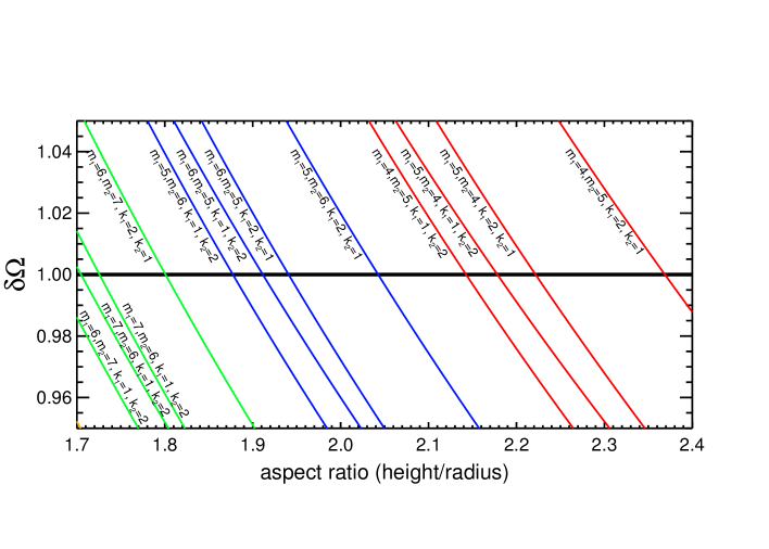
Figure 2: Frequency difference $\delta\Omega$ in dependence of the aspect ratio $\Gamma$ for two free Kelvin modes which fulfill $\delta m=1$ and $\delta k=1$. The crossings of the curves with the horizontal black line at $\delta\Omega=1$ mark the aspect ratio at which triadic resonances can be expected.

These aspect ratios at which $\delta\Omega=1$ are listed in table 1 together with the corresponding frequencies of the resonant free Kelvin modes.

$m_{a}$	$k_{a}$	$m_{b}$	$k_{b}$	$\Omega_{a}$	$\Omega_{b}$	$\Gamma$
6	1	7	2	0.3825	-0.6175	1.67420
7	1	6	2	0.3356	-0.6644	1.70478
7	2	6	1	0.6494	-0.3506	1.72568
6	2	7	1	0.6956	-0.3045	1.80074
5	1	6	2	0.3888	-0.6113	1.87742
6	1	5	2	0.3352	-0.6648	1.91146
6	2	5	1	0.6489	-0.3511	1.94082
5	2	6	1	0.7013	-0.2987	2.04266
4	1	5	2	0.3974	-0.6026	2.14270
5	1	4	2	0.3350	-0.6649	2.17832
5	2	4	1	0.6485	-0.3515	2.22216
4	2	5	1	0.7092	-0.2907	2.36888

Table 1: Possible triadic resonances with $\delta m=1$, $\delta k=1$ and $\delta\Omega=1$ and corresponding aspect ratios. Negative frequencies present pro-grade modes and positive frequencies denote retrograde modes. Only the first radial wave number has been considered for each value of $m$ and $k$.

A triad is always formed by free Kelvin modes consisting of one prograde and one retrograde mode [1993PhFl....5..677W]. Note that the frequencies of free Kelvin modes that constitute different triads often are close (if we restrict to triads with $k_{a}=1$ and $k_{b}=2$, see table 1) making it difficult to reliably identify individual Kelvin modes in realistic setups with potential frequency shifts due to viscous and/or non-linear effects.

3 Numerical model

We conduct numerical simulations in a cylindrical geometry with the code SEMTEX that applies a spectral element Fourier approach for the numerical solution of the Navier-Stokes equation [2004JCoPh.197..759B]. In order to simplify the implementation of the precessional forcing we switch to the precessional frame in which the precession is stationary and the cylinder rotates with a frequency $\Omega_{\rm{c}}$. Thus only a term for the Coriolis force appears in the Navier-Stokes equation which now reads

$$\frac{\partial\mbox{\boldmath$u$}}{\partial t}+\mbox{\boldmath$u$}\cdot\nabla\mbox{\boldmath$u$}+2\mbox{\boldmath$\Omega$}_{\rm{p}}\times\mbox{\boldmath$u$}=-\nabla P+\nu\nabla^{2}\mbox{\boldmath$u$}.$$ (12)

Due to the rotation of the cylinder in the precessing frame the boundary conditions for the azimuthal flow change to $u_{\varphi}=r\Omega_{\rm{c}}$ (at endcaps and sidewall) whereas no-slip conditions are still applied for $u_{z}$ and $u_{r}$.

The problem is described by four parameters, the Reynolds number defined with the angular velocity of the container ${\rm{Re}}=\Omega_{\rm{c}}R^{2}/\nu$, the precession ratio (or Poincaré number) ${\rm{Po}}=\displaystyle{\Omega_{\rm{p}}}/{\Omega_{\rm{c}}}$, the aspect ratio $\Gamma=H/R$ and the precession angle $\alpha$ with $\cos\alpha={\mbox{\boldmath$\Omega$}_{\rm{p}}\cdot\mbox{\boldmath$\Omega$}_{\rm{c}}}/{|\mbox{\boldmath$\Omega$}_{\rm{p}}||\mbox{\boldmath$\Omega$}_{\rm{c}}|}$. In the present study, we keep the precession ratio fixed at ${\rm{Po}}=0.0141$ and the precession angle is set to $\alpha=\pi/2$. All simulations are performed at ${\rm{Re}}=6500$ except for one run at ${\rm{Re}}=10000$ to briefly examine the impact of increasing ${\rm{Re}}$. The aspect ratio is varied in the range $\Gamma\in[1.7;2.4]$ in order to find the container geometry for which individual modes or triads become resonant.

4 Results

4.1 Pattern of the total flow

The simulations are started from an initial state with pure solid-body rotation $\mbox{\boldmath$u$}=r\widehat{\mbox{\boldmath$e$}}_{\varphi}$. After switching on the Coriolis force at $t=0$ the fluid shows a direct response in form of a large scale mode with $m=1$. In dependence of the aspect ratio this is only a transient state until after a finite time (which may take up to 1000 rotation periods or more) a quasi-steady state is reached. The typical flow pattern for $\Gamma=2$ and ${\rm{Re}}=6500$ is presented in figure 3 where the nested isosurfaces show a snapshot of the axial velocity $u_{z}$ at 30% (60%, 90%) of its maximum value.

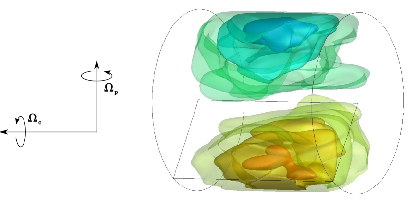
Figure 3: Volume rendering of the axial velocity $u_{z}$ at ${\rm{Re}}=6500$ and $\Gamma=2$. The nested isosurfaces show $u_{z}$ at 30% (60%, 90%) of its maximum value. An animation of the flow’s behavior in the statistically stationary state is available at https://www.hzdr.de/db/VideoDl?pOid=45098.

The flow is clearly dominated by a velocity mode with $m=1$ and $k=1$. This is the primary Kelvin mode driven by the precessional forcing. Superimposed on the $m=1$ mode we see some non-axisymmetric (time-dependent) disturbances that will be analyzed below.

4.2 Kinetic energy

4.2.1 Forced mode

In the following we discuss the behavior of the flow by means of azimuthal Fourier modes $\mbox{\boldmath$\widetilde{u}$}_{m}(r,z)$ with the total flow given by $\mbox{\boldmath$u$}(r,z,\varphi)={2\pi}/({N_{\varphi}}+1)\sum_{m=0}^{N_{\varphi}}\widetilde{\mbox{\boldmath$u$}}_{m}(r,z)e^{im\varphi}$. Figure 4 shows the history of the kinetic energy of the $m=1$ mode for different aspect ratios.

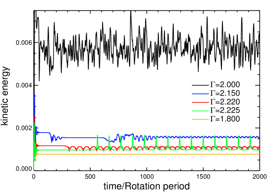
Figure 4: Kinetic energy of the $m=1$ mode versus time for various $\Gamma$. Note the qualitative diversity for different aspect ratios.

A final state arises either after a short transitional period ($\Gamma=2.000$) or after one or more bifurcations (see e.g. the blue curve for $\Gamma=2.150$). The final state can be chaotic ($\Gamma=2.000$, black curve), oscillatory ($\Gamma=2.15$, blue), quasi-periodic with collapses ($\Gamma=2.2$, red), quasi-periodic with bursts ($\Gamma=2.225$, green) or stationary ($\Gamma=1.8$, yellow). We also find transient periods with constant energy (e.g. $\Gamma=2.15$ for $t=300...600$), and it may take up to 1200 revolutions of the cylinder ($\Gamma=2.15$, blue curve) till a final quasi-stationary state is reached. This saturation time also depends on the Reynolds number and decreases with increasing ${\rm{Re}}$.

The bifurcations shown by the $m=1$ mode go along with the emergence of non-axisymmetric modes with $m\geq 2$ (figure 5). These modes become unstable only after quite a long time, e.g., for $\Gamma=1.825$ it takes up to $600$ rotation periods of the cylinder till modes with $m\geq 2$ start to grow, and it may take up to twice that time till a quasi-steady state is reached. The non-axisymmetric modes with $m\geq 2$ essentially proceed similar to the behavior of the $m=1$ mode, i.e., we see a chaotic behavior when the $m=1$ mode behaves chaotic ($\Gamma=2.0$, figure 5, central panel) and we see periodic growth and decay when the $m=1$ mode is periodic ($\Gamma=1.825$, top panel in figure 5 and $\Gamma=2.200$, bottom panel in figure 5). In the periodic regime the amplitude of the energy oscillations of the modes with $m\geq 2$ is rather large so that the kinetic energy may vary in time by more than one order of magnitude.

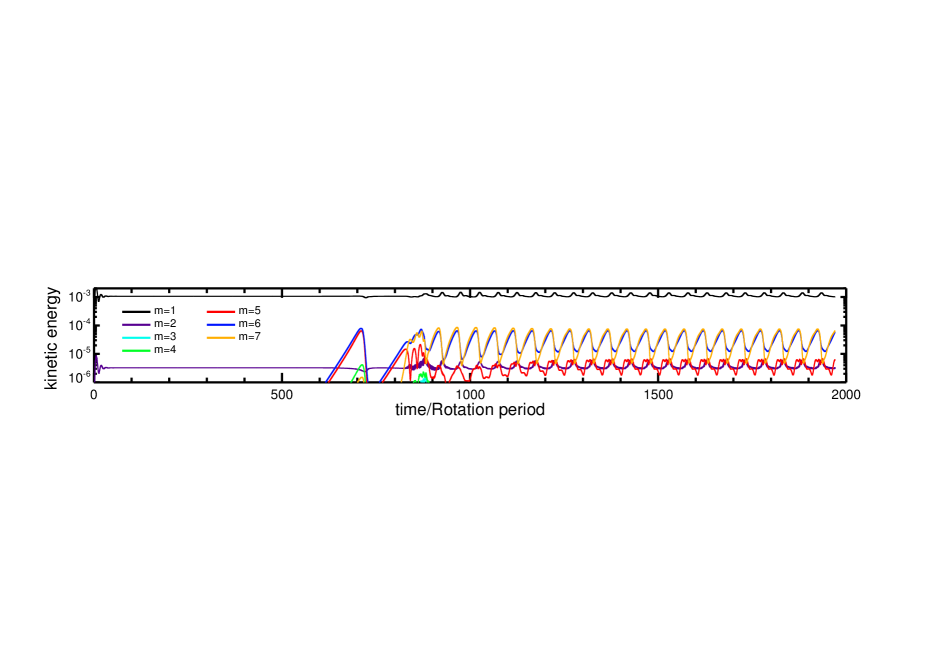
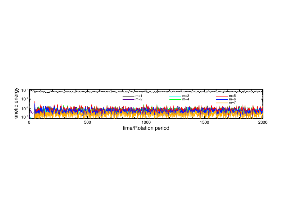
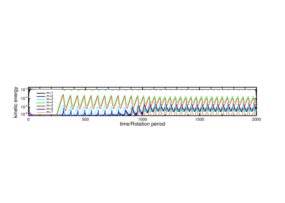
Figure 5: Temporal behavior of the modes with $m=1,\dots,7$. From top to bottom: $\Gamma=1.825,2.000,2.200$. Note the different vertical scale for $\Gamma=2.000$ (central panel).

In the following we compare analytic expressions for the energy of the forced mode with the time-averaged energy taken from the quasi-stationary period of the final state in our simulations. This comparison is only partly justified because the analytical expressions are based on a number of serious simplifications, such as the linearization of the Navier-Stokes equation, the limit ${\rm{Po}}\rightarrow 0$, and the neglect of the time dependent part of the Coriolis force which is justified only for small precession angles $\alpha$. Furthermore, the final state in our simulations is instable and additional caution is advised when comparing simulations with a linear time independent solution. Nevertheless, such an analysis is helpful to identify the regimes in which, e.g., a maximum response of the flow can be expected, or to localize the aspect ratios at which triadic resonances are possible.

Analytically, the energy of the forced Kelvin mode is given by [2012JFM...709..610L]

$$E_{m=1}=\Gamma^{2}\sum\limits_{j}\frac{(k\pi/\Gamma)^{2}+\frac{1}{2}(2-\Omega_{j})}{\Omega_{j}^{2}(4-\Omega_{j}^{2})}|A_{j}|^{2}J_{1}^{2}(\lambda_{j})$$ (13)

where the index $j$ now denotes a combination of the axial wave number $k$ and the radial wave number $n$, and $A_{j}$ is the inviscid linear amplitude given by (7) with the azimuthal wave number fixed at $m=1$. $A_{j}$ can also be calculated by the method of 2012JFM…709..610L which includes viscosity and is valid at and off the resonance. However, in that case equation (13) is accurate only up to an error of $O({\rm{Re}}^{-\frac{1}{2}})$ since equation (13) does not consider the energy from the flow in the boundary layers. Figure 6 shows the time-averaged energy taken from the simulations (black curve) compared with the analytic solutions (green curve, inviscid solution and blue curve, viscous solution). For the calculation of the analytical solutions equation (13) is truncated at $n=6$ and $k=6$ which is sufficient to reach convergence (off-resonance in the inviscid case) and avoids the occurrence of too many resonances in the inviscid case (green curve) which anyway are suppressed in the more realistic viscous or non-linear computations.

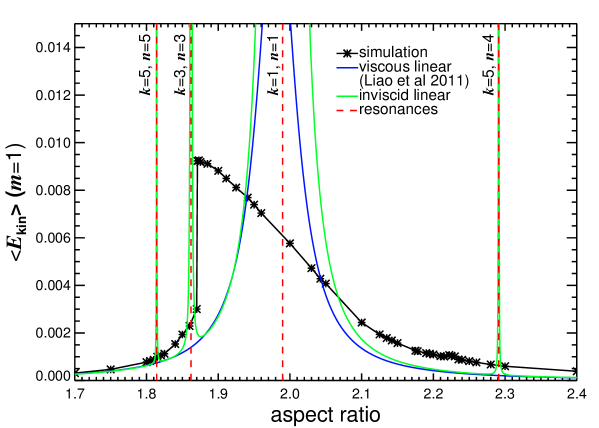
Figure 6: Time-averaged kinetic energy of the fundamental mode ($m=1$) versus aspect ratio. ${\rm{Re}}=6500,{\rm{Po}}=0.014,\alpha=\pi/2$. The dashed red lines denote the resonances with larger $k$ and/or $n$. For the computation of the energy, equation (13) has been truncated at $k=6$ and $n=6$ (with prograde and retrograde modes respectively). Note that the inviscid solution (green curve) diverges at the resonances whereas the viscous solution has a finite maximum of $E_{\rm{kin}}^{\rm{max}}\approx 0.021$ at $\Gamma\approx 1.9814$.

Comparing the numerical solutions (black curve) with the linear solutions we see significant deviations around the primary resonance ($k=1,n=1$, $\Gamma_{\!\!\rm{res}}\approx 1.9898$) while outside of this regime the agreement of all curves remains good (say for $\Gamma\mathrel{\mathchoice{\vbox{\offinterlineskip\halign{\hfil$\displaystyle#$\hfil\cr<\cr\sim\cr}}}{\vbox{\offinterlineskip\halign{\hfil$\textstyle#$\hfil\cr<\cr\sim\cr}}}{\vbox{\offinterlineskip\halign{\hfil$\scriptstyle#$\hfil\cr<\cr\sim\cr}}}{\vbox{\offinterlineskip\halign{\hfil$\scriptscriptstyle#$\hfil\cr<\cr\sim\cr}}}}1.85$ and for $\Gamma\mathrel{\mathchoice{\vbox{\offinterlineskip\halign{\hfil$\displaystyle#$\hfil\cr>\cr\sim\cr}}}{\vbox{\offinterlineskip\halign{\hfil$\textstyle#$\hfil\cr>\cr\sim\cr}}}{\vbox{\offinterlineskip\halign{\hfil$\scriptstyle#$\hfil\cr>\cr\sim\cr}}}{\vbox{\offinterlineskip\halign{\hfil$\scriptscriptstyle#$\hfil\cr>\cr\sim\cr}}}}2.05$). Two key features characterize the behavior of the mean energy in our simulations. On the one hand we see a clear shift of the maximum to smaller aspect ratios and the maximum energy arises rather close to the aspect ratio expected for the resonance with $k=3$ and $n=3$. However, this resonance is suppressed by viscous effects and we do not see strong contributions with $k=3$ and/or $n=3$ in our simulations (see also section 4.5.1). Therefore the correlation is either coincidental or we have to assume an indirect impact of the ($k=3,n=3$) resonance. The second scenario is supported by the abrupt transition from the absolute maximum to a rather low energy state right below $\Gamma\approx 1.871$. This jump is also connected to a modification of the character of the $m=1$ mode which changes its behavior below $\Gamma\approx 1.86$ from the chaotic regime to the periodic regime. Abrupt transitions of the energy of higher azimuthal modes can also be seen at the other (theoretical) resonances of the forced mode ($k=5,n=5$ and, a little further away $k=5,n=4$, see figure 6) which will be revisited in the next paragraph. Beside the shift of the maximum to smaller aspect ratios the energy obtained in the simulations remains considerably smaller compared to the linear viscous solution. The maximum of the energy based on the amplitude of 2012JFM…709..610L is $E_{\rm{kin}}^{\rm{max}}\approx 0.021$ (at $\Gamma\approx 1.9814$) which is roughly two times larger than the maximum kinetic energy obtained in our simulations ($E_{\rm{kin}}^{\rm{max}}\approx 0.0093$ at $\Gamma=1.871$). The differences are not surprising because the prerequisites for the computation of the amplitudes $A_{j}$ are not well met in our simulations. In particular, we observe a significant impact of non-linear interactions in the simulations in terms of higher non-axisymmetric modes and the forming of an azimuthal shear flow that both draw energy from the forced $m=1$ mode.

4.2.2 Higher azimuthal wave numbers

We only find higher non-axisymmetric modes with a noteworthy amount of energy between $\Gamma\approx 1.81$ and $\Gamma\approx 2.24$. This corresponds approximately to the regime in which the energy of the $m=1$ mode deviates from the linear prediction (see previous paragraph). For the sake of brevity we will call this regime the non-linear regime, assuming that the higher modes are triggered by non-linear effects. The kinetic energy of the modes with $m\geq 2$ is roughly 2 orders of magnitude smaller than the energy of the forced mode but essential characteristics such as the maximum at $\Gamma=1.871$ and the abrupt drop of kinetic energy below this threshold are also reflected in the behavior of the higher non-axisymmetric modes (figure 7).

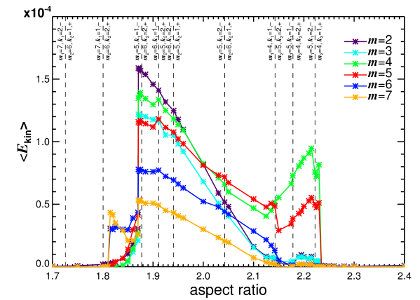
Figure 7: Time-averaged kinetic energy of azimuthal modes with $m\geq 2$. ${\rm{Re}}=6500,{\rm{Po}}=0.014,\alpha=\pi/2$. The vertical lines indicate the aspect ratios for which triadic resonances could be expected according to the dispersion relation (4). The labels denote the corresponding azimuthal and axial wave numbers with $-$ ($+$) marking retrograde (prograde) modes.

The sudden drop of the energy for $\Gamma\leq 1.871$ pertains to all modes which indicates that this breakdown might be a global flow property that is not connected to an individual mode.

A similar steep decrease of energy can also be found on the two outer edges of the non-linear regime. It is striking that all the abrupt transitions are close to theoretical resonances of the forced mode ($k=3,n=3\Rightarrow\Gamma_{\rm{res}}\approx 1.8621,k=5,n=5\Rightarrow\Gamma_{\rm{res}}\approx 1.8142$, and with some greater distance $k=5,n=4\Rightarrow\Gamma_{\rm{res}}\approx 2.2911$ , see figure 6). These resonances are, however, suppressed and cannot be directly observed in the simulations. So far, we cannot conclude whether the correlation of the energy jumps and the occurrence of (theoretical) resonances is a coincidence, or whether they may be some systematic relationship.

Away from the primary resonance of the forced mode we find two further regimes with local maxima of the higher modes. For $1.80\mathrel{\mathchoice{\vbox{\offinterlineskip\halign{\hfil$\displaystyle#$\hfil\cr<\cr\sim\cr}}}{\vbox{\offinterlineskip\halign{\hfil$\textstyle#$\hfil\cr<\cr\sim\cr}}}{\vbox{\offinterlineskip\halign{\hfil$\scriptstyle#$\hfil\cr<\cr\sim\cr}}}{\vbox{\offinterlineskip\halign{\hfil$\scriptscriptstyle#$\hfil\cr<\cr\sim\cr}}}}\Gamma\mathrel{\mathchoice{\vbox{\offinterlineskip\halign{\hfil$\displaystyle#$\hfil\cr<\cr\sim\cr}}}{\vbox{\offinterlineskip\halign{\hfil$\textstyle#$\hfil\cr<\cr\sim\cr}}}{\vbox{\offinterlineskip\halign{\hfil$\scriptstyle#$\hfil\cr<\cr\sim\cr}}}{\vbox{\offinterlineskip\halign{\hfil$\scriptscriptstyle#$\hfil\cr<\cr\sim\cr}}}}1.85$ we see a narrow window with the maximum around $\Gamma\approx 1.825$ in which the $m=6$ and $m=7$ mode dominate (blue and yellow curve in figure 7). Likewise, but more explicit, we find the $m=4$ and $m=5$ mode becoming dominant for $2.05\mathrel{\mathchoice{\vbox{\offinterlineskip\halign{\hfil$\displaystyle#$\hfil\cr<\cr\sim\cr}}}{\vbox{\offinterlineskip\halign{\hfil$\textstyle#$\hfil\cr<\cr\sim\cr}}}{\vbox{\offinterlineskip\halign{\hfil$\scriptstyle#$\hfil\cr<\cr\sim\cr}}}{\vbox{\offinterlineskip\halign{\hfil$\scriptscriptstyle#$\hfil\cr<\cr\sim\cr}}}}\Gamma\mathrel{\mathchoice{\vbox{\offinterlineskip\halign{\hfil$\displaystyle#$\hfil\cr<\cr\sim\cr}}}{\vbox{\offinterlineskip\halign{\hfil$\textstyle#$\hfil\cr<\cr\sim\cr}}}{\vbox{\offinterlineskip\halign{\hfil$\scriptstyle#$\hfil\cr<\cr\sim\cr}}}{\vbox{\offinterlineskip\halign{\hfil$\scriptscriptstyle#$\hfil\cr<\cr\sim\cr}}}}2.25$ with a maximum around $\Gamma\approx 2.2$ (green and red curves in figure 7).

The local maxima around $\Gamma\approx 1.825$ and $\Gamma\approx 2.2$ for Fourier modes with $\delta m=1$ indicate the presence of corresponding triadic resonances and roughly agree with predictions from the dispersion relation (see table 1 and figure 2). From the linear predictions we would also expect triads with $m=5$ and $m=6$ in the intermediate regime (for $1.85<\Gamma<2.05$) but obviously there are other flow contributions with at least comparable energy which may disguise the energetic signature of the involved free Kelvin modes (e.g., we see relatively high energies of the $m=4$ and the $m=5$ modes, whereas in comparison the $m=6$ mode is clearly suppressed).

4.3 Spatial Structure of the Fourier modes

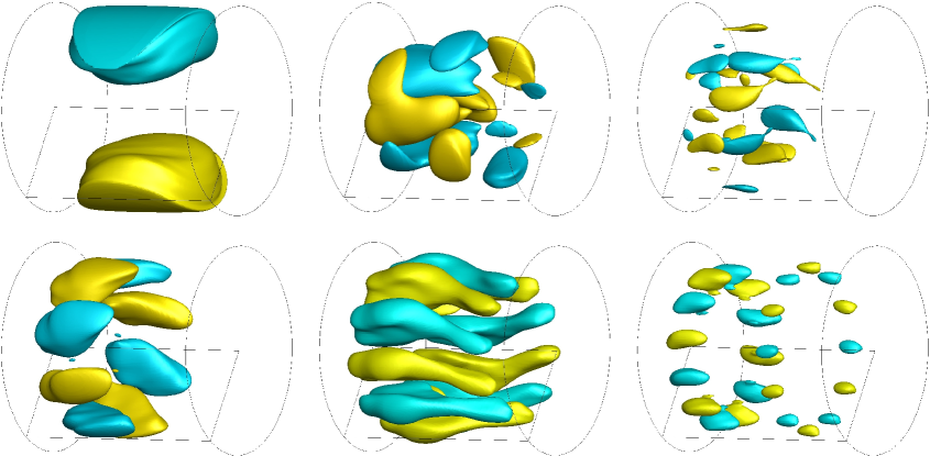
Figure 8: Snapshot of the axial velocity field $u_{z}$ filtered to $m=1\dots 6$ (upper left to lower right) for $\Gamma=2$ (isosurface at 50% of the respective maximum value). An animation of the flow pattern is available at https://www.hzdr.de/db/VideoDl?pOid=45104. The temporal behavior of the modes $m=2$ and $m=3$ is complex and chaotic. The modes $m=4,5$ and $6$ show a more regular behavior essentially resulting from the superimposition of free Kelvin modes with $k=1$ and $k=2$. ${\rm{Re}}=6500,{\rm{Po}}=0.014,\alpha=\pi/2$.

A qualitative impression of the flow structure is provided by isosurfaces of the individual Fourier modes of the axial velocity shown in figure 8 for $\Gamma=2$ (for an impression of the temporal behavior see the snapshots of the $m=5$ mode in figure 9 and the movie at https://www.hzdr.de/db/VideoDl?pOid=45104). The $m=1$ mode is obviously dominated by a $k=1$ contribution and shows comparatively small variations in time. Regarding the higher non-axisymmetric modes we see a complex pattern for the $m=2$ and $m=3$ mode with irregular temporal and spatial fluctuations and a more regular behavior of the modes $m=4,5$ and $6$ with typical signatures of $k=1$ and $k=2$. It is striking that the $m=6$ mode, which should become resonant around $\Gamma\approx 2$, remains weak compared to the $m=4$ or the $m=5$ mode.

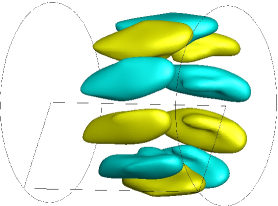
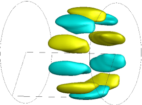
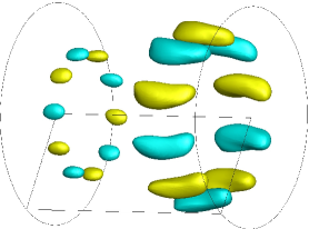
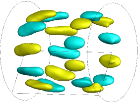
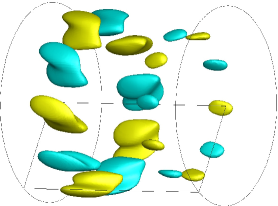
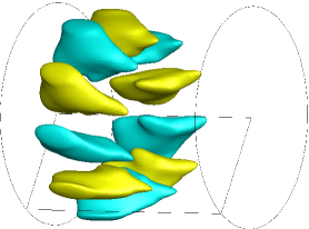
Figure 9: Time series of the $m=5$ mode that visualizes the axial symmetry breaking. The isosurfaces show $\widetilde{u}_{m=5,z}(r,\varphi,z)$ at 50% of its maximum value at various characteristic time steps (form upper left to lower right: t=2617.5418, 2617.8489, 2618.0845, 2618.1958, 2618.8738, 2618.9599 (time in units of the rotation time); note that the time gaps are not equidistant).

The amplitude of the individual contributions with $m=4,5,6$ varies in time and the resulting flow perpetually changes its axial structure. The azimuthal mode resulting from the superposition of $k=1$ and $k=2$ contributions has a distinct and time dependent asymmetry with respect to the equatorial plane of the cylinder, so that the associated flow is concentrated alternately in both halves of the cylindrical container (see time series of the $m=5$ mode in figure 9). The typical timescale for this process is of the order of the rotation period $2\pi/\Omega_{\rm{c}}$ but we can not derive a reliable periodicity from our simulations.

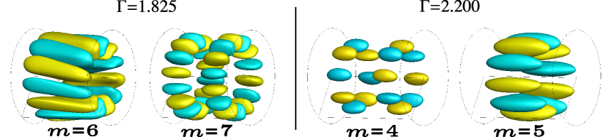
Figure 10: Snapshots of the structure of the axial velocity field for different Fourier modes. Left: $\Gamma=1.825$, dominated by $m=6,k=1$ and $m=7,k=2$. Right: $\Gamma=2.200$, dominated by $m=4,k=2$ and $m=5,k=1$. In both cases these modes represent the dominant contributions of the non-axisymmetric modes with $m\geq 2$ (see figure 13 below and animation at https://www.hzdr.de/db/VideoDl?pOid=45105).

Away from the primary resonance of the forced mode the structure of higher azimuthal modes is much more regular and – except for periodic variations of amplitude – essentially remains constant over time. Figure 10 shows the dominant azimuthal modes (beyond $m=1$) at $\Gamma=1.825$ ($m=6$ and $m=7$) and at $\Gamma=2.200$ ($m=4$ and $m=5$). In both cases, the axial behavior of the modes shows clear indications of axial wave numbers $k=1$ and/or $k=2$ and we will show below that these modes indeed fulfill all conditions of equation (11) and thus constitute triadic resonances. In contrast to the behavior at $\Gamma=2$, the geometric structure of the dominant modes exhibits only minor temporal variations except strong oscillations of the amplitude (see animation at https://www.hzdr.de/db/VideoDl?pOid=45105).

4.4 Radial dependence

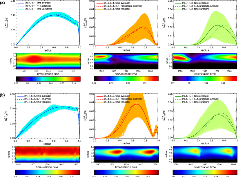
Figure 11: Radial dependence of the axial velocity decomposed into the dominant Fourier- and axial modes according to equation (14). (a) $\Gamma=1.825$, from left to right: ($m=1,k=1$), ($m=6,k=1$) and ($m=7,k=2$), (b) $\Gamma=2.200$, from left to right: ($m=1,k=1$), ($m=4,k=2$) and ($m=5,k=1$). The solid thick curves show the temporal average and the weakly saturated colored curves show radial profiles at different time steps representing the temporal variations. The thick dashed curves denote the theoretical profiles from the linear inviscid solutions ($\propto J_{m}(\lambda_{j}r)$, see equation (5)). The colored contour plots below each profile show the corresponding variation of the radial profiles in time.

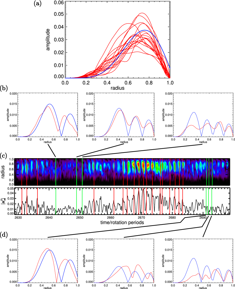
Figure 12: Snapshots of radial profiles $\widehat{{u}}_{m,z}^{k}(r)$ with $m=5$ and $k=1$ at $\Gamma=2$. (a) snapshots taken at local maxima of the ($m=5,k=1$) mode dominated by $n=1$ (marked by the the vertical red lines in panel (c)). The blue curve represents the analytical behavior $\propto J_{5}(\lambda_{j}r)$ with $\lambda_{j}$ the first root of the dispersion relation. (b), (d): snapshots of the radial profiles that match to a higher radial wave number. The red curves denote the numerical data and the blue curves denote a fit $\propto J_{5}(\lambda_{j}r)$ with $\lambda_{j}$ corresponding to the second, third and fourth root of the dispersion relation (4). The corresponding time steps are marked by the green lines in panel c. (c) temporal variations of the radial profiles and of the amplitude $|\widehat{u}^{1}_{5,z}|$ at $r=0.67$.

In order to quantify the visual observations made in the previous section and to estimate amplitude and frequency of individual Kelvin modes we use a discrete sine-transformation (DST) applied to each Fourier mode

$$\mbox{\boldmath$\widehat{u}$}^{k}_{m}(r)=\sum\limits_{q=1}^{N_{z}}\mbox{\boldmath$\widetilde{u}$}_{m}(r,z_{n})\sin\left(\frac{qk\pi}{N_{z}+1}\right)$$ (14)

with $N_{z}$ the number of points in axial direction. Figure 11 shows radial profiles for the dominant contributions to the axial velocity at $\Gamma=1.825$ (a) and at $\Gamma=2.200$ (b) where we only present the three leading modes for each case. The solid thick curves present the time average and the bright colors in the background represent the variation of the radial profiles in time. For comparison, the thick dashed curves show the analytical behavior $\propto J_{m}(\lambda_{j}r)$ predicted by the linear in-viscid approximation (5) with $\lambda_{j}$ the first root of the dispersion relation (4). The differences between the numerical data and the analytical curves are surprisingly small with deviations mainly in the boundary layers which can be explained by the different boundary conditions for the simulations (no slip) and the in-viscid solution (free slip). Except for (considerable) changes in the amplitude the pattern of the radial profiles exhibits only minor temporal changes and shows no significant contributions from higher radial modes (see color coded contour plots in figure 11 that show the variations of the radial profiles in time).

The behavior becomes more complex at $\Gamma=2$ at which we see many modes with different $m$ and $k$ with nearly the same amplitude and clear changes in the radial structure. Figure 12 shows characteristic radial profiles for the mode ($m=5,k=1$) and their temporal behavior as a typical example. The amplitude exhibits considerable fluctuations and, unlike in the previous cases, we see additional changes in the radial structure. When the amplitude is around a (local) maximum, the radial velocity profile is in accordance with a wavenumber that corresponds to the first root of the dispersion relation and the radial profiles can nicely be described by a function $\propto J_{5}(\lambda_{1}r)$ (see red curves in figure 12a). However, when the amplitude is weak we see clear signatures of higher radial wave numbers (see figure 12 b and d). Even though the higher radial modes remain weak, they might represent a channel for the transfer of energy from the (periodically occurring) maxima of a mode into smaller scales.

4.5 Amplitudes and frequencies

4.5.1 Height equal diameter $(\Gamma=2)$

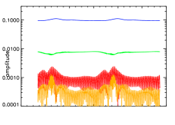
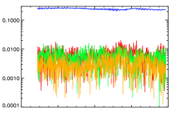
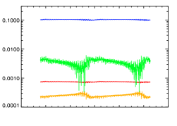
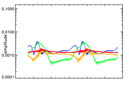
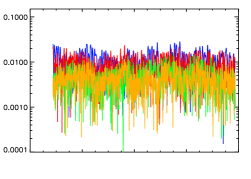
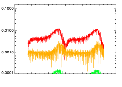
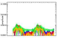
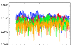
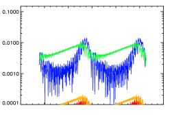
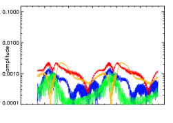
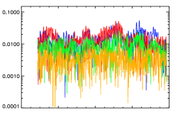
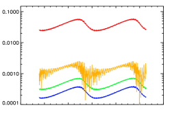
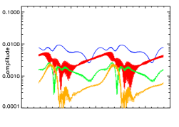
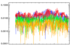
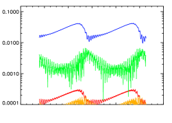
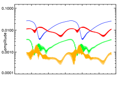
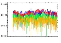
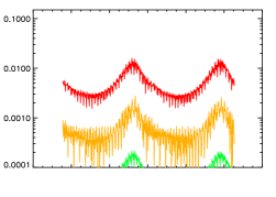
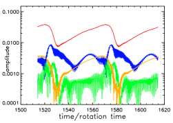
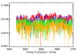
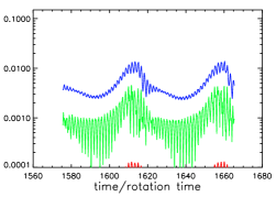
Figure 13: Temporal behavior of the amplitude of the flow $\widehat{{u}}^{k}_{m,z}$ at $r=0.67$ decomposed into Fourier- and axial modes with $m=1...7$ (from top to bottom) and $k=1...4$ (blue, red, green, yellow curve). From left to right: $\Gamma=1.825$, $\Gamma=2.0$ and $\Gamma=2.2$.

${\rm{Re}}$	$m$	$k$	$\max|u_{m}^{k}|$	$\Omega_{\rm{num}}$	$\Omega_{\rm{theo}}$
6500	$1$	$1$	0.2673	$-1.0000$	$-1.0000$ (forced)
	$3$	$1$	$0.0412$	$+0.2911$	$+0.3342$ (for $n=2$)
	$3$	$2$	$0.0266$	$+0.3154$	$+0.3333$ (for $n=5$)
	$4$	$1$	$0.0536$	$+0.0357$	no corresponding mode
	$4$	$2$	$0.0525$	$+0.3593$	$+0.3647$ (for $n=4$)
	$5$	$1$	$0.0491$	$+0.2278$	$+0.2030$ (for $n=3$)
	$5$	$2$	$0.0578$	$+0.4692$	$+0.5157$ (for $n=2$)
	$6$	$1$	$0.0392$	$+0.2006$	$+0.1868$ (for $n=3$)
	$6$	$2$	$0.0391$	$+0.6239$	$+0.6309$ (for $n=1$)
10000	$1$	$1$	0.2775	$-1.0000$	$-1.0000$ (forced)
	$3$	$1$	0.0329	$+0.3090$	$+0.3342$ (for $n=2$)
	$3$	$2$	0.0302	$+0.3013$	$+0.3333$ (for $n=5$)
	$4$	$1$	0.0562	$+0.1687$	$+0.1532$ (for $n=5$)
	$4$	$2$	0.0420	$+0.3511$	$+0.3647$ (for $n=4$)
	$5$	$1$	0.0570	$+0.2001$	$+0.2030$ (for $n=3$)
	$5$	$2$	0.0574	$+0.5168$	$+0.5157$ (for $n=2$)
	$6$	$1$	0.0417	$+0.3452$	$+0.3204$ (for $n=1$)
	$6$	$2$	0.0437	$+0.6410$	$+0.6309$ (for $n=1$)

Table 2: Amplitudes and frequencies from the simulations at $\Gamma=2$. Only modes with well-defined drift behavior are listed. The columns denote (from left to right): Reynolds number, azimuthal wave number, axial wave number, maximum of the amplitude, azimuthal drift frequency from the numerical data, and theoretical frequency from the dispersion relation (4) for larger radial wave numbers $n$ that fit best to the observed frequencies.

Figure 13 shows the temporal behavior of $|{\widehat{u}}_{m,z}^{k}|$ at $r=0.67$ for $m=1$ to $m=7$ (from top to bottom) and for $k=1$ to $k=4$ (blue, red, green, yellow curve). The peak values of the amplitudes are additionally listed in table 2 ($\Gamma=2$) and in table 3 ($\Gamma=1.825$ and $\Gamma=2.2$) together with the frequencies obtained from the time derivative of the azimuthal phase of each mode. Note that we only list modes with a regular behavior of the frequencies, i.e., contributions which exhibit a steady and unique azimuthal drift that allows a conclusive computation of the time derivative of the azimuthal phase. The results quantitatively complement the observations made in the previous paragraph. For $\Gamma=2$ (central column and table 2) we see a dominant forced mode with $m=1$ and $k=1$ and the contributions with $k>1$ are negligible (smaller by a factor of 20). The higher azimuthal modes ($m=2\dots 7$) reach approximately $10\%$ of the amplitude of the $m=1$ mode with $k=1$ and $k=2$ slightly prevailing over $k=3$ and $k=4$. A striking property of the flow at $\Gamma=2$ is the common orientation of the azimuthal drift motion of all modes (see table 2). We only find modes with a retrograde azimuthal drift so no combination is possible that fulfills the requirements for a triadic resonance (in all cases $\delta\Omega\neq 1$, see table 2). The presence of distinct frequency signals that fit to higher radial modes (which however are hardly evident in the radial profiles for the ($m=5,k=1$) mode, see figure 12) shows that there must be further contributions with chaotic behavior which are probably dominant and having no regular azimuthal drift.

We also performed simulations at a slightly larger Reynolds number ${\rm{Re}}=10000$ (at $\Gamma=2$) and found only minor changes with respect to the run at ${\rm{Re}}=6500$ except for the modes $(m=4,k=1)$ and $(m=6,k=1)$ which have lower frequencies at ${\rm{Re}}=6500$. However, so far our data is not sufficient to explain the impact of ${\rm{Re}}$ on the drift frequencies or to establish a conclusive scaling towards more realistic ${\rm{Re}}$ that will be reached in the experiment. Hence, we refrain from any further discussion of the properties of the flow at larger ${\rm{Re}}$.

4.5.2 Triadic resonances at $\Gamma=1.825$ and $\Gamma=2.200$

The behavior of the amplitude confirms the modified characteristics of the flow when the forced mode is off-resonance ($\Gamma=1.825$, left column in figure 13, or $\Gamma=2.2$, right column in figure 13; see also table 3). For $\Gamma=2.200$ we find a well-defined single triadic resonance with unique wave numbers ($m=4,k=2$ and $m=5,k=1$) and frequencies ($\Omega_{a}=-0.6368$ and $\Omega_{b}=0.3632$). These values fulfill the conditions for a triadic resonance and are quite close to the theoretical values obtained from the dispersion relation (4) (see table 3).

$\Gamma$	$m$	$k$	$\max|u_{m}^{k}|$	$\Omega_{\rm{num}}$	$\Omega_{\rm{theo}}$
1.825	$1$	$1$	$0.1113$	$-1.0000$	$-1.0000$ (forced mode)
	$6$	$1$	$0.0272$	$-0.2979$	$-0.3045$ (at $\Gamma=1.80074$)
	$7$	$2$	$0.0382$	$+0.7010$	$+0.6956$ (at $\Gamma=1.80074$)
	$5$	$1$	$0.0094$	$-0.2596$	$-0.3511$ (at $\Gamma=1.94082$)
	$6$	$2$	$0.0144$	$+0.7405$	$+0.6489$ (at $\Gamma=1.94082$)
2.200	$1$	$1$	$0.1095$	$-1.0000$	$-1.0000$ (forced mode)
	$4$	$2$	$0.0596$	$-0.6368$	$-0.6650$ (at $\Gamma=2.17832$)
	$5$	$1$	$0.0423$	$+0.3632$	$+0.3350$ (at $\Gamma=2.17832$)

Table 3: Amplitudes and frequencies from the simulations for the dominant modes at $\Gamma=1.825$ and $\Gamma=2.200$. The columns denote (from left to right): aspect ratio, azimuthal wave number, axial wave number, maximum of the amplitude, azimuthal drift frequency from numerical data, and theoretical frequency from the dispersion relation (4) at the aspect ratio at which the linear inviscid approximation predicts a triadic resonance (always supposing a radial wave number corresponding to the first root of the dispersion relation which is confirmed in figure 11).

The emergence of a triadic resonance is less explicit at $\Gamma=1.825$. However, at this aspect ratio we find even two triadic resonances (see figure 13) with $(m,k)=(6,1)$ and $(7,2)$ and a second resonance with $(m,k)=(5,1)$ and $(6,2)$ (with much weaker amplitude, see table 3). In all cases the amplitude of the free modes that constitute a triadic resonance strongly oscillates with a maximum of up to 50% of the forced mode ($\Gamma=2.2,m=4,k=2$) which corresponds to roughly 6% of the angular velocity of the cylindrical container.

4.6 Azimuthal shear flow

The growth of the triads goes along with a growth of an axisymmetric azimuthal shear flow that is mostly geostrophic (see left panel in figure 14). The axisymmetric mode emerges with a slight delay with respect to the free Kelvin modes which indicates a saturation process by a detuning of the resonance frequencies (see right panel in figure 14). The induced axialsymmetric flow component is negative on average and, hence, causes a breaking of the solid body rotation which increases with increasing precession ratio. In the extreme case the breaking of the induced axisymmetric flow entirely cancels the solid body rotation, giving the impression that in the laboratory frame the cylindrical container is rotating around a standing fluid [johann]. This effect is closely connected to the abrupt transition to a chaotic flow which takes place at a critical precession ratio [johann, 2014PhFl...26e1703K].

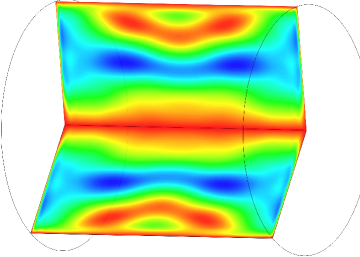
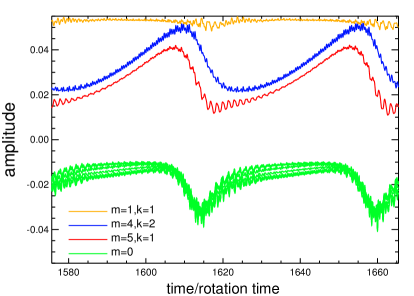
Figure 14: Left: Pattern of the induced azimuthal shear flow at $\Gamma=2.2$. Right: Temporal development of the amplitude at $r=0.67$ of the azimuthal shear flow (green curve), the free Kelvin modes (red and green curve) and the forced mode (yellow curve).

5 Conclusions

We performed numerical simulations of a precession driven flow in cylindrical geometry. The simulations confirm that the energy that can be injected via precessional forcing is very sensitive to the aspect ratio of the cylindrical container. Significant contributions of higher non-axisymmetric components appear only in a limited range of aspect ratios (for $\Gamma\in[1.81;2.24]$) and it turns out that in that regime the behavior of the forced mode (with $m=1$) cannot be described by a linear theory. Nevertheless, in all cases the forced Kelvin mode ($m=1$) dominates and free Kelvin modes with higher azimuthal wave number appear as distortions of the forced mode. The maximum response of the flow takes place at $\Gamma_{\rm{max}}\approx 1.871$ which is remarkable far away from the resonance predicted by the linear in-viscid approximation (at $\Gamma=1.98982$). At the resonance maximum our results yield an amplitude for the $z$-component of the flow of $|{{u}}^{\rm{max}}_{z}|\approx 0.27$, which – assuming isotropy – roughly agrees with the estimations of leorat2. The amplitude of the forced mode decreases with increasing distance from the resonance maximum, and in the regimes with triadic resonances, we still observe values of $|{{u}}^{\rm{max}}_{z}|\approx 0.10$ (in terms of the azimuthal velocity of the container). In real units (assuming $\Omega_{\rm{c}}=2\pi\cdot 10\mbox{Hz}$ and $R=1\,{\rm{m}}$) this would correspond to fluid velocities of $15\,\mbox{m/s}$ (at resonance) and $6\,\mbox{m/s}$ (off resonance) which is of the same order as the typical flow speed in the Riga dynamo experiment. Regarding the higher Kelvin modes, the saturated amplitudes of the strongest free Kelvin modes are mostly independent of the forced mode and achieve values of about $0.05$ to $0.06$ in terms of the angular velocity of the container corresponding to $\sim 3.5\,{\rm{m}}/{\rm{s}}$ in the experiment.

At the aspect ratio envisaged for the experiment ($\Gamma=2$ with $H=2\,{\rm{m}}$ and $R=1\,{\rm{m}}$) we may expect an energy of the fluid flow at roughly two thirds of the maximum value at the optimum aspect ratio ($\Gamma=1.871$). However, this optimum aspect ratio probably depends on the Reynolds number and on the forcing, so that we believe that the chosen geometry for the dynamo experiment is a good compromise to ensure an efficiently driven fluid flow in a container with a ratio of diameter to height that at least approximately reflects the geometry of planetary bodies.

Although at present we do not know whether the flow fields that emerge in our simulations will be able to drive a dynamo, we may try to estimate typical magnetic field strengths that can be expected in the planned dynamo experiment. We assume a saturation of the magnetic energy at roughly $5\%$ of the kinetic energy of the hydrodynamic flow which is substantiated by the saturation behavior of the Riga dynamo [2008CRPhy...9..721G]. We further presuppose that the internal velocity caused by the precessional forcing linearly scales with the rotation of the container (and hence with ${\rm{Re}}$) and assume an angular velocity of $\Omega_{\rm{c}}=2\pi\cdot 10\,\mbox{Hz}$, a radius $R=1\,\mbox{m}$, a height $H=2\,\mbox{m}$ and a density of liquid sodium of $\rho\approx 930\,\mbox{kg/m}^{3}$ (at $\sim\!400\,{\rm{K}}$). After the change over to real units the kinetic energy obtained in our simulations at $\Gamma=2$ ($E_{\rm{kin}}\approx 0.006$) corresponds approximately to a magnetic field strength $B\approx\sqrt{0.05\mu_{0}\rho E_{\rm{kin}}\Omega_{\rm{c}}^{2}}\approx 40\,\mbox{mT}$. This is in the range of the Riga dynamo which is not particularly surprising since the typical velocities obtained in our simulations indeed match the velocity arising in the Riga dynamo. However, given that the corresponding $m=1$ mode has produced no dynamo in the kinematic simulations it might be more realistic to refer to the free Kelvin modes with higher $m$ which have less kinetic energy. In that case the typical magnetic field strength amounts to only $B\approx 5\,\mbox{mT}$ which, however, is still in the range of the values obtained at the Von-Kármán-Sodium dynamo [2007PhRvL..98d4502M]. We expect a stronger response and hence a larger saturation field strength for increasing ${\rm{Po}}$, at least as long as we remain below the critical Poincare number for the sudden transition to a chaotic state johann${\rm{Po}}^{\rm{crit}}\approx 0.0725$ at ${\rm{Re}}=5.65\times 10^{5}$, see. However, unless we know whether or not the precession driven flow will have the right structure and sufficient magnitude to excite dynamo action at all, these estimations are only useful to demonstrate that the reference values assumed for the planned dynamo experiment will allow magnetic fields with a reasonable field strength.

Regarding the structure of the flow, we find various manifestations of non-axisymmetric contributions in terms of free Kelvin modes with higher azimuthal wave numbers $m$. We find free Kelvin modes in resonance with the forced mode only when the forced mode is sufficiently far away from its primary resonance, i.e., when the amplitude of the forced mode is not too strong. Triadic resonances can be clearly identified using a combined Fourier-Discrete Sine transformation in the azimuth and along the axis with structure and frequencies close to predictions from linear theory. Actually, we were also expecting triads around $\Gamma\approx 2$ with $m=5$ and $m=6$. Indeed, we do find patterns of free Kelvin modes in that regime, but no combination of them satisfies the triadic resonance conditions. Instead, we see free Kelvin modes solely with retrograde drift motion and for each azimuthal wavenumber $m$ the contributions with $k=1$ and $k=2$ are approximately of equal strength so that in sum we see a clear breaking of the equatorial symmetry of the flow. This symmetry breaking has been essential for the functioning of a dynamo in simulations of 2005PhFl…17c4104T in a precessing sphere whereas it seemed less important in the direct numerical simulations of 2011PhRvE..84a6317N. However, preliminary kinematic dynamo simulations we conducted recently with an analytic flow of Kelvin modes suggest that the joint appearance of contributions with $k=1$ and $k=2$ considerably facilitates the occurrence of dynamo action.

The triadic instability requires a rather long time to emerge and saturates to a final state with slow periodic growth and decay. This period is likely related to the precession time scale but a conclusive correlation requires further simulations at different ${\rm{Po}}$. The periodic growth followed by a fast decay of the free Kelvin modes in the regime with triadic resonances reminds of the so called resonant collapse [1970JFM....40..603M, 1992JFM...243..261M]. However, in our simulations the energy is essentially distributed among very few, large scale modes. These modes are the fundamental forced mode and two free Kelvin modes that establish the triad and an axisymmetric, essentially geostrophic mode. We do not spot any turbulence-like behavior during the decay of the free Kelvin modes, i.e. there is no transition from the dominance of the large scale mode into small scale turbulent flow which would be characteristic for the collapse phenomenon. This behavior might change when the Reynolds number approaches larger (i.e. more realistic) values. This is substantiated by the simulations at $\Gamma=2$. Here we see no triadic resonance, but rather a quasi-periodic occurrence of free Kelvin modes that exhibit a trend towards larger radial wave numbers during their decay which may represent (part of) a cascade to small scale structures.

In principle the occurrence of very few dominant modes calls for a low-dimensional model. However, the ansatz (9) used in this study to explain the occurrence of triadic resonances is too simplistic to allow for a reasonable description of the non-linear behavior and the saturation obtained in the simulations presented above. A more sophisticated approach is presented by FLM:7951619 who use a low-dimensional model with four coupled ordinary differential equations that describe the amplitude of the forced mode, the free Kelvin modes and an axisymmetric geostrophic mode. This model allows for saturation via the axisymmetric mode and for a reinforcement of the forced mode by the free Kelvin modes and qualitatively reproduces the results obtained in our simulations. However, in order to yield a quantitative agreement, advanced models are still required.

References

References

- [1] \harvarditemAldridge \harvardand Lumb19871987Natur.325..421A Aldridge K D \harvardand Lumb L I 1987 Nature 325, 421–423.
- [2] \harvarditemBao \harvardand Pascal19971997bao Bao G \harvardand Pascal M 1997 Arch. Appl. Mech. 67(6), 407–421.
- [3] \harvarditemBlackburn \harvardand Sherwin20042004JCoPh.197..759B Blackburn H M \harvardand Sherwin S J 2004 J. Comp. Phys. 197, 759–778.
- [4] \harvarditemD. Breuer et al.20102010SSRv..152..449B Breuer D, Labrosse S \harvardand Spohn T 2010 Space Sci. Rev. 152, 449–500.
- [5] \harvarditemM. Breuer et al.20102010GeoJI.183..150B Breuer M, Manglik A, Wicht J, Trümper T, Harder H \harvardand Hansen U 2010 Geophys. J. Int. 183, 150–162.
- [6] \harvarditemBusse19681968JFM….33..739B Busse F H 1968 J. Fluid Mech. 33, 739–751.
- [7] \harvarditemConnaughton et al.20102010colm Connaughton C P, Nadiga B T, Nazarenko S V \harvardand Quinn B E 2010 J. Fluid Mech. 654, 207–231.
- [8] \harvarditemDavidson20142014GeoJI.198.1832D Davidson P A 2014 Geophys. J. Int. 198, 1832–1847.
- [9] \harvarditemDudley \harvardand James19891989RSPSA.425..407D Dudley M L \harvardand James R W 1989 Proc. R. Soc. Lond. Ser. A 425, 407–429.
- [10] \harvarditemErnst-Hullermann et al.2011hullermann Ernst-Hullermann J, Harder H \harvardand Hansen U 2011 Geophys. J. Int. 195(3), 1395–1405.
- [11] \harvarditemGailitis et al.20082008CRPhy…9..721G Gailitis A, Gerbeth G, Gundrum T, Lielausis O, Platacis E \harvardand Stefani F 2008 C. R. Phys. 9, 721–728.
- [12] \harvarditemGailitis et al.20002000PhRvL..84.4365G Gailitis A, Lielausis O, Dement’ev S, Platacis E, Cifersons A, Gerbeth G, Gundrum T, Stefani F, Christen M, Hänel H \harvardand Will G 2000 Phys. Rev. Lett. 84, 4365–4368.
- [13] \harvarditemGans19701970JFM….41..865G Gans R F 1970 J. Fluid Mech. 41, 865–872.
- [14] \harvarditemGans19711971JFM….45..111G Gans R F 1971 J. Fluid Mech. 45, 111–130.
- [15] \harvarditemGiesecke et al.20152014arXiv1411.1195G Giesecke A, Albrecht T, Gerbeth G, Gundrum T \harvardand Stefani F 2015 Magnetohydrodynamics 51(2), 293–302.
- [16] \harvarditemGreenspan1968greenspan Greenspan H P 1968 The theory of rotating fluids Cambridge University Press.
- [17] \harvarditemHerault et al.2015johann Herault J, Gundrum T, Giesecke A \harvardand Stefani F 2015 Phys. Fluids 0(0), 0–0. submitted.
- [18] \harvarditemHerreman \harvardand Lesaffre20112011JFM…679…32H Herreman W \harvardand Lesaffre P 2011 J. Fluid Mech. 679, 32–57.
- [19] \harvarditemKerswell19991999JFM…382..283K Kerswell R R 1999 J. Fluid Mech. 382, 283–306.
- [20] \harvarditemKing et al.20102010GGG….11.6016K King E M, Soderlund K M, Christensen U R, Wicht J \harvardand Aurnou J M 2010 Geochem. Geophy. Geosy. 11, 6016.
- [21] \harvarditemKobine19951995JFM…303..233K Kobine J J 1995 J. Fluid Mech. 303, 233–252.
- [22] \harvarditemKong et al.20142014PhFl…26e1703K Kong D, Liao X \harvardand Zhang K 2014 Phys. Fluids 26(5), 051703.
- [23] \harvarditemKrauze2010krauze Krauze A 2010 Magnetohydrodynamics 46(3), 271–280.
- [24] \harvarditemLagrange et al.20082008PhFl…20h1701L Lagrange R, Eloy C, Nadal F \harvardand Meunier P 2008 Phys. Fluids 20(8), 081701.
- [25] \harvarditemLagrange et al.2011FLM:7951619 Lagrange R, Meunier P, Nadal F \harvardand Eloy C 2011 J. Fluid Mech. 666, 104–145.
- [26] \harvarditemLéorat et al.2003leorat1 Léorat J, Rigaud F, Vitry R \harvardand Herpe G 2006 Magnetohydrodynamics 39(3), 321–326.
- [27] \harvarditemLéorat2006leorat2 Léorat J 2006 Magnetohydrodynamics 42(2/3), 143–151.
- [28] \harvarditemLiao \harvardand Zhang20122012JFM…709..610L Liao X \harvardand Zhang K 2012 J. Fluid Mech. 709, 610–621.
- [29] \harvarditemLin et al.20142014PhFl…26d6604L Lin Y, Noir J \harvardand Jackson A 2014 Phys. Fluids 26(4), 046604.
- [30] \harvarditemLorenzani \harvardand Tilgner20032003JFM…492..363L Lorenzani S \harvardand Tilgner A 2003 J. Fluid Mech. 492, 363–379.
- [31] \harvarditemMalkus19681968Sci…160..259M Malkus W V R 1968 Science 160, 259–264.
- [32] \harvarditemManasseh19921992JFM…243..261M Manasseh R 1992 J. Fluid Mech. 243, 261–296.
- [33] \harvarditemManasseh19941994JFM…265..345M Manasseh R 1994 J. Fluid Mech. 265, 345–370.
- [34] \harvarditemManasseh19961996JFM…315..151M Manasseh R 1996 J. Fluid Mech. 315, 151–173.
- [35] \harvarditemMcEwan19701970JFM….40..603M McEwan A D 1970 J. Fluid Mech. 40, 603–640.
- [36] \harvarditemMeunier et al.20082008JFM…599..405M Meunier P, Eloy C, Lagrange R \harvardand Nadal F 2008 J. Fluid Mech. 599, 405–440.
- [37] \harvarditemMiller19821982miller Miller M C 1982 J. Guid. Control Dynam. 5(2), 151–157.
- [38] \harvarditemMoffatt1970FLM:383564 Moffatt H K 1970 J. Fluid Mech. 44, 705–719.
- [39] \harvarditemMonchaux et al.20072007PhRvL..98d4502M Monchaux R, Berhanu M, Bourgoin M, Moulin M, Odier P, Pinton J F, Volk R, Fauve S, Mordant N, Pétrélis F, Chiffaudel A, Daviaud F, Dubrulle B, Gasquet C, Marié L \harvardand Ravelet F 2007 Phys. Rev. Lett. 98(4), 044502.
- [40] \harvarditemMouhali et al.20122012ExFl…53.1693M Mouhali W, Lehner T, Léorat J \harvardand Vitry R 2012 Exp. Fluids 53, 1693–1700.
- [41] \harvarditemNore et al.20112011PhRvE..84a6317N Nore C, Léorat J, Guermond J L \harvardand Luddens F 2011 Phys. Rev. E 84(1), 016317.
- [42] \harvarditemPfeiffer19741974pfeiffer Pfeiffer F 1974 Ing. Arch. 43(5), 306–316.
- [43] \harvarditemRossby19391939rossby Rossby C G 1939 J. Mar. Res. 2(1), 38–55.
- [44] \harvarditemStefani et al.20152014arXiv1410.8373S Stefani F, Albrecht T, Gerbeth G, Giesecke A, Gundrum T, Herault J, Nore C \harvardand Steglich C 2015 Magnetohydrodynamics 51(2), 275–284.
- [45] \harvarditemStefani et al.2012stefani Stefani F, Eckert S, Gerbeth G, Giesecke A, Gundrum T, Steglich C, Weier T \harvardand Wustmann B 2012 Magnetohydrodynamics 48(1), 103–114.
- [46] \harvarditemStewartson \harvardand Roberts19631963JFM….17….1S Stewartson K \harvardand Roberts P H 1963 J. Fluid Mech. 17, 1–20.
- [47] \harvarditemStieglitz \harvardand Müller20012001PhFl…13..561S Stieglitz R \harvardand Müller U 2001 Phys. Fluids 13, 561–564.
- [48] \harvarditemThomson1880Kelvin Thomson W 1880 Philos. Mag. 10, 152–165.
- [49] \harvarditemTilgner1998tilgner98 Tilgner A 1998 Studia geoph. et geod. 42, 232–238.
- [50] \harvarditemTilgner20052005PhFl…17c4104T Tilgner A 2005 Phys. Fluids 17(3), 034104.
- [51] \harvarditemWaleffe19931993PhFl….5..677W Waleffe F 1993 Phys. Fluids 5, 677–685.
- [52] \harvarditemWu \harvardand Roberts20092009GApFD.103..467W Wu C C \harvardand Roberts P 2009 Geophys. Astrophys. Fluid Dynam. 103, 467–501.
- [53]