Polymer quantization and the saddle point approximation of partition functions

Abstract

The saddle point approximation of the path integral partition functions is an important way of deriving the thermodynamical properties of black holes. However, there are certain black hole models and some mathematically analog mechanical models for which this method cannot be applied directly. This is due to the fact that their action evaluated on a classical solution is not finite and its first variation does not vanish for all consistent boundary conditions. These problems can be dealt with by adding a counterterm to the classical action, which is a solution of the corresponding Hamilton-Jacobi equation.

In this work we study the effects of polymer quantization on a mechanical model presenting the aforementioned difficulties and contrast it with the above counterterm method. This type of quantization for mechanical models is motivated by the loop quantization of gravity which is known to play a role in the thermodynamics of black hole systems.

The model we consider is a nonrelativistic particle in an inverse square potential, and analyze two polarizations of the polymer quantization in which either the position or the momentum is discrete. In the former case, Thiemann’s regularization is applied to represent the inverse power potential but we still need to incorporate the Hamilton-Jacobi counterterm which is now modified by polymer corrections. In the latter, momentum discrete case however, such regularization could not be implemented. Yet, remarkably, owing to the fact that the position is bounded, we do not need a Hamilton-Jacobi counterterm in order to have a well-defined saddle point approximation. Further developments and extensions are commented upon in the discussion.

I Introduction

Two major open problems in theoretical physics regard the nature of spacetime: on one hand there is the issue of singularities, beyond which classical general relativity cannot be continued, and, on the other, one finds the divergent high energy behavior of field theories. A quantum theory of gravity is expected to have a bearing on both of these problems. For instance, loop quantum gravity Rovelli (2004); Thiemann (2007); Gambini and Pullin (2011); Bojowald (2011); Rovelli and Vidotto (2014) has been shown indeed to replace the big bang of general relativistic homogeneous cosmological models by a bounce Bojowald (2001); Ashtekar et al. (2006) and quantum field theory in such a scenario Thiemann (1998a) is rather different from usual fixed background field theory. Moreover, it has also provided a specific account for black hole entropy Ashtekar et al. (1998).

Now to investigate the behavior of some simple systems under this approach it is possible to use polymer quantum mechanics, a finite number of degrees of freedom scheme including some of the loop quantum gravity techniques Ashtekar et al. (2003). This simplified approach has been applied to some systems to contrast their behavior with their usual Schrödinger quantization and its relation with the latter either as a continuum limit Corichi et al. (2007a, b) or as a low energy approximation Flores-Gonzĺez et al. (2013). Furthermore, for the case of fields on a fixed background this technique has been applied to each of its infinite modes as a candidate to explore their high energy behavior Hossain et al. (2010); García-Chung and Morales-Técotl (2014). Even higher order derivative models have been given consideration along these lines recently Cumsille et al. (2015). With the exception of Husain and Winkler (2003) that advanced a path integral version of polymer quantum mechanics, most work on these lines adopted a Hamiltonian scheme. This changed recently: a path integral approach was considered Ashtekar et al. (2009, 2010a, 2010b) in order to provide a more detailed link between loop quantum cosmology and the covariant spin foam models Rovelli and Vidotto (2014), and a polymer path integral in quantum field theory and its relation to Lorentz invariance has also been studied in (Kajuri, 2015). Also the Feynman formula for other mechanical examples has been worked out Parra and Vergara (2014), and explicit polymer propagators have been obtained Morales-Técotl et al. (2015). An interesting aspect of this so-called Feynman approach is that semiclassical approximations can be at hand to investigate important gravitating systems through the saddle point approximation of its path integral description. In fact, the Euclidean path integral is specially useful in studying the thermodynamics of systems such as black holes since there it is interpreted as the partition function of the system in a canonical ensemble.

Let us consider the semiclassical approximation for a system with the Euclidean path integral

$$\mathcal{Z}=\int\prod_{j}\mathscr{D}\phi_{j}\exp\left(-\frac{1}{\hbar}S_{E}[\phi_{j}]\right),$$ (1)

in which $\phi_{j}$ are the fields of the theory and $S_{E}$ is its Euclidean action. Given that one can expand the action around the classical solutions $\phi_{j}\big{|}_{cl}$ as

$$S_{E}\left[\left.\phi_{j}\right|_{cl}+\delta\phi_{j}\right]=S_{E}\left[\left.\phi_{j}\right|_{cl}\right]+\delta S_{E}\left[\left.\phi_{j}\right|_{cl}+\delta\phi_{j}\right]+\frac{1}{2}\delta^{2}S_{E}\left[\left.\phi_{j}\right|_{cl}+\delta\phi_{j}\right]+\cdots,$$ (2)

one can then substitute this into (1); by keeping only up to the quadratic term, one gets

$$\mathcal{Z}\approx\exp\left(-\frac{1}{\hbar}S_{E}\left[\left.\phi_{j}\right|_{cl}\right]\right)\int\prod_{j}\mathscr{D}\phi_{j}\exp\left(-\frac{1}{2\hbar}\delta^{2}S_{E}\left[\left.\phi_{j}\right|_{cl}+\delta\phi_{j}\right]\right),$$ (3)

which is the saddle point approximation to the model that gives us access to the semiclassical information about the system.

More precisely, a saddle point approximation (3) of (1) is possible only if the following conditions are met:

1. The variational principle is well-defined: $S_{E}$ must be functionally differentiable for all the variations of the fields and compatible with the boundary and falloff conditions of the fields, so that any boundary term must vanish by virtue of these conditions; thus we can write $\delta S_{E}=\int d^{n}x\frac{\delta S_{E}}{\delta\phi_{j}}\delta\phi_{j}$. This is needed so that one is able to

   1. expand $S_{E}$ as in (2) around an arbitrary configuration $\phi_{0}$ using the functional derivatives,

   2. find the classical solutions by setting $\delta S_{E}=0$,

   3. perform the expansion (2) specifically around the classical solutions $\left.\phi_{j}\right|_{cl}$.

2. Given condition 1, then $S_{E}$ on classical solutions must remain finite, i.e., $S_{E}\big{|}_{\delta S_{E}=0}<\infty$.

3. Given conditions 1 and 2, the Gaussian integral $\int\prod_{j}\mathscr{D}\phi_{j}\exp\left(-\frac{1}{2\hbar}\delta^{2}S_{E}\left[\left.\phi_{j}\right|_{cl}+\delta\phi_{j}\right]\right)$ also must remain finite.

4. Since there is a minus sign in the exponent of (1), we should also have $\delta^{2}S_{E}\left[\left.\phi_{j}\right|_{cl}+\delta\phi_{j}\right]>0$ so that the classical solutions give the dominant contribution to the saddle point approximation.

The physical reason behind the above conditions is that for a semiclassical approximation, the most important contribution comes from the classical solutions, and thus everything is expanded around such a trajectory. The rest of the terms become less and less important, and thus we only need to keep the perturbative terms up to the quadratic term, which gives us the nonclassical contributions.

There are, however, some important systems for which these conditions are not met and thus access to the semiclassical approximation via the saddle point method is not possible (Regge and Teitelboim, 1974; Gibbons and Hawking, 1977; Liebl et al., 1997; Papadimitriou and Skenderis, 2005; McNees, 2005; Mann and Marolf, 2006). Among these systems are a class of two-dimensional (2D) dilatonic gravitational systems, including models like CGHS (Callan-Giddings-Harvey-Strominger model) (Callan et al., 1992) and 3+1 spherically symmetric, which have black hole solutions and many other related interesting properties. This class can be described by the generic action (Grumiller and McNees, 2007)

$$S=-\frac{1}{16\pi G_{2}}\int_{\mathcal{M}}d^{2}x\sqrt{-g}\left[\Phi R-U(\Phi)\nabla_{a}\Phi\nabla^{a}\Phi-2V(\Phi)\right]-\frac{1}{8\pi G_{2}}\int_{\partial\mathcal{M}}dx\sqrt{q}\Phi K.$$ (4)

Here $\Phi$ is the dilaton field, and $U(\Phi)$ and $V(\Phi)$ are model-dependent functions of the dilaton field. The latter is called the dilaton potential. The boundary term is the equivalent of the Gibbons-Hawking-York term (York, 1972) in this theory in which $K$ is the trace of the extrinsic curvature of the boundary manifold.

To see the problem with saddle point approximation, we consider the on-shell variation of the action (Grumiller and McNees, 2007)

$$\delta S\big{|}_{cl}=\int_{\partial\mathcal{M}}dx\sqrt{q}\left(\Xi^{ab}\delta q_{ab}+\Upsilon_{\Phi}\delta\Phi\right).$$ (5)

It can be shown that this variation does not vanish in some of the models of this generic class. This is basically due to the fact that in these models, the coefficients of the variations of the spatial metric $q_{ab}$ and the dilaton $\Phi$ in the above expression, diverge more rapidly than the variations themselves fall off. This might look odd since the presence of the Gibbons-Hawking-York (GHY) term is supposed to guarantee the well-posedness of the variational principle in these kinds of theories. Notice, however, that the presence of the GHY terms is to let us avoid prescribing Neumann boundary conditions for the metric, i.e. it cancels all the variations $\delta(\partial_{a}g_{bc})$ that come from the bulk term. It does not guarantee that the Dirichlet boundary conditions on the dilaton field lead to a well-posed variational principle. Also it may not be helpful in dealing with issues emanating from falloff conditions of the dilaton field. It is these types of boundary and falloff conditions that contribute to the problem here.

In some of the submodels of this class, even if the variational principle is well defined, the on-shell value of the action diverges, especially due to the falloff conditions on the dilaton field and its value on the boundary. So the saddle point approximation collapses for these types of models.

Since as mentioned above, one important use of saddle point approximation is to study the thermodynamics of black holes, not being able to make such an approximation for this class of 2D models is a significant shortcoming. Luckily there is a common and rather generic method of fixing this problem that consists of the addition of a boundary counterterm to $S_{E}$, which not only makes the action functionally differentiable for all boundary and falloff conditions, but also renders the on-shell value of the action finite. It turns out that this boundary counterterm is a solution to the Hamilton-Jacobi equation of the system (Grumiller and McNees, 2007). The action that is the sum of (4) and the Hamilton-Jacobi boundary term is called the improved action. An interesting observation is that the improved action actually gives the correct thermodynamics for the system (Grumiller and McNees, 2007).

In this paper, we investigate the behavior of the polymer path integral quantization of a mechanical model that in the usual path integral quantization suffers from the aforementioned ill-defined semiclassical approximation. Whether this fixes the problem, and whether we need a Hamilton-Jacobi counterterm, it is relevant to know how the polymer approach changes the partition function for such systems and, perhaps, the thermodynamics of some of the 2D black holes. The present work is a first step in this direction, and we study a simpler analog model of the aforementioned 2D class, namely, a particle in an inverse square potential, that has the same technical problems within the usual nonpolymer path integral quantization. Let us notice that the Hamiltonian polymer quantization of a particle subject to a Coulomb (Husain et al., 2007) and an inverse squared Kunstatter et al. (2009) potential, respectively, have been considered previously. Hence, our work complements these studies.

The paper is organized as follows. In Sec. II, we introduce the analog model and describe the saddle point issue for this case. Then we recall its solution through the application of the Hamilton-Jacobi method. In Sec. III, we polymerize this analog model in a polarization where the position $q$ is discrete. We will see that in this polarization, one still needs to add a counterterm to the action to get a new well-defined action suitable for saddle point approximation. However, we show that this counterterm and the bulk action are both modified by polymer quantization. In Sec. IV we propose an effective potential for the semiclassical version of the analog model in a polarization with discrete momentum $p$. We then describe how this effective potential does not require the addition of any counterterm to the action. Finally we summarize and make our concluding remarks in Sec. V. Details of the calculations are given in the appendixes at the end of the paper.

II Analog mechanical model and its improved action

There are several types of simpler analog models that exhibit the aforementioned ill-defined semiclassical approximation. One such class of models corresponds to single particle systems in half-binding potentials $W$ (Grumiller, 2007). We choose a simple system in this class with an inverse square potential with the Newtonian action (the subscripts $N$ and $E$ stand for Newtonian and Euclidean, respectively)

$$S_{N}=\int_{t_{i}=0}^{t_{f}=\infty}dt\,L_{N}=\int_{t_{i}=0}^{t_{f}=\infty}dt\left(\frac{m}{2}\left(\frac{dq}{dt}\right)^{2}-W(q)\right),\,\,\,\,\,\,\,\,\,\,\,\,\,\,\,\,\,\,\,\,\,\,\,W(q)=\frac{k}{q^{2}}$$ (6)

and corresponding Euclidean action (by a Wick rotation $t\rightarrow\tau=it$), $S_{N}=iS_{E}$,

$$S_{E}=\int_{\tau_{i}=i0}^{\tau_{f}=i\infty}d\tau\,L_{E}=\int_{\tau_{i}=i0}^{\tau_{f}=i\infty}d\tau\left(\frac{m}{2}\left(\frac{dq}{d\tau}\right)^{2}+W(q)\right).$$ (7)

The Newtonian equation of motion is

$$m\frac{d^{2}}{dt^{2}}q=-\frac{\partial W}{\partial q}\left(=\frac{2k}{q^{3}}\right),$$ (8)

which under a Wick rotation becomes

$$m\frac{d^{2}}{d\tau^{2}}q=\frac{\partial W}{\partial q}\left(=-\frac{2k}{q^{3}}\right).$$ (9)

Let us see the problems of the saddle point approximation for this analog model. First, we consider the variation of the Euclidean action

$$\delta S_{E}=\left[\frac{\partial L_{E}}{\partial\frac{d}{d\tau}q}\delta q\right]_{0}^{\infty}+\int_{0}^{\infty}d\tau\left(-\frac{d}{d\tau}\frac{\partial L_{E}}{\partial\frac{d}{d\tau}q}+\frac{\partial L_{E}}{\partial q}\right)\delta q.$$ (10)

If the boundary term does not vanish for all the variations of $\delta q$ compatible with the boundary and falloff conditions, then the action is not functionally differentiable. It turns out that this is the case. At $\tau=it_{i}=i0$, since the value of $q$ is finite, we have $\delta q=0$. However, at $\tau=it_{f}=i\infty$, since $q\rightarrow\infty$, the condition $\delta q\big{|}_{\infty}\neq 0$ is also allowed; i.e., any two trajectories do not necessarily coincide at infinity, and yet they both tend to infinite values. Thus the action is not functionally differentiable with this boundary condition.

The common way to overcome this issue is to add a boundary term $-B$ to the action that cancels out the boundary term present in (10). Clearly the variation of the boundary term should obey $\delta B=\frac{\partial L}{\partial\frac{d}{d\tau}q}\delta q=p\delta q$. It just happens that Hamilton’s principal function $G$ has exactly this property. This is because we have

$$\delta G(q,t)=\frac{\partial G}{\partial q}\delta q=p\delta q=\frac{\partial L}{\partial\frac{d}{d\tau}q}\delta q.$$ (11)

Hence we conclude that by adding

$$-B=-G$$ (12)

to the action, it becomes functionally differentiable. Such an action is called the “improved” action,

$$\Gamma[q]=S_{E}-\left.G(q,t)\right|_{0}^{t_{f}}=\int_{0}^{t_{f}}dt\left(\dfrac{m\dot{q}^{2}}{2}+\dfrac{k}{q^{2}}\right)-\left.G(q,t)\right|_{0}^{t_{f}}.$$ (13)

Clearly, the variation of (13) yields

$$\delta S_{E}=\int_{0}^{\infty}d\tau\left(-\frac{d}{d\tau}\frac{\partial L_{E}}{\partial\frac{d}{d\tau}q}+\frac{\partial L_{E}}{\partial q}\right)\delta q+\left[\left(\frac{\partial L_{E}}{\partial\frac{d}{d\tau}q}-\frac{\partial G}{\partial q}\right)\delta q\right]_{0}^{\infty}=\int_{0}^{\infty}d\tau\left(-\frac{d}{d\tau}\frac{\partial L_{E}}{\partial\frac{d}{d\tau}q}+\frac{\partial L_{E}}{\partial q}\right)\delta q.$$ (14)

Next, we consider the Euclidean action itself. We would like to show that even if the action is functionally differentiable, the value of the Euclidean action on classical solutions is not finite, and that the addition of $G$ to the action, makes it finite. Assuming for the moment that $S_{E}$ is functionally differentiable, using the Leibniz rule on the kinetic term and then computing the action on the classical solutions, we can write

$$S_{E}\big{|}_{q_{cl}}=\left[\frac{m}{2}q_{cl}\frac{dq}{d\tau}\bigg{|}_{cl}\right]_{\tau=i0}^{\tau=i\infty}+\int_{i0}^{i\infty}d\tau\left(\left.-\frac{m}{2}q_{cl}\frac{d^{2}q}{d\tau^{2}}\right|_{cl}+\frac{k}{q_{cl}^{2}}\right).$$ (15)

Using (9) and the form of the classical solution $q_{cl}(\tau)$, the integral turns out to be finite and of order $\pi$. On the other hand, it can clearly be seen that the boundary term above (or its Newtonian counterpart) diverges, since at $\tau\rightarrow\infty$ (or $t\rightarrow\infty$) the system behaves as a free particle, $\frac{dq}{d\tau}|_{cl}$ (or $\frac{dq}{dt}|_{cl})$ is constant, and $q_{cl}\rightarrow\infty$. Thus the action evaluated on classical solutions is not finite,

$$S_{E}\big{|}_{q_{cl}}\rightarrow\infty.$$ (16)

These results show that the direct saddle point approximation cannot be performed for this system.

Now let us see what is the form of $G$ and how it makes the action, evaluated on classical solutions, finite. The variable $t$ is used from now on, both as Euclidean or Newtonian time, depending on the context. Since $G$ in (13) is a solution of the Hamilton-Jacobi equation, we have

$$H\left(q,\dfrac{\partial G}{\partial q}\right)+\dfrac{\partial G}{\partial t}=0.$$ (17)

To find the explicit form of $G$ we need to solve (17). Considering the Euclidean Hamiltonian

$$H=\frac{p^{2}}{2m}-\frac{k}{q^{2}},$$ (18)

and noting that $p=\frac{\partial G}{\partial q}$, the Eq. (17) becomes

$$\frac{1}{2m}\left(\frac{\partial G}{\partial q}\right)^{2}-\frac{k}{q^{2}}+\frac{\partial G}{\partial t}=0.$$ (19)

Since the Hamiltonian does not depend explicitly on $t$, Eq. (17) implies that the derivative $\nicefrac{{\partial G}}{{\partial t}}$ must be a constant in time and is actually the negative of the energy of the system $H=E$. So one can make an additive separation of the variables in $G$ as

$$G(q,E,t)=\Omega(q,E)-Et,$$ (20)

which turns (19) into

$$\frac{1}{2m}\left(\frac{\partial\Omega}{\partial q}\right)^{2}-\frac{k}{q^{2}}=E$$ (21)

or

$$\left(\frac{\partial\Omega}{\partial q}\right)=\frac{\sqrt{2m}\sqrt{Eq^{2}+k}}{q}.$$ (22)

This can be integrated to yield $\Omega$, which together with (20) leads to

$$G(q,t)=c_{0}-Et+\sqrt{2}\sqrt{m}\sqrt{Eq^{2}+k}-\sqrt{2}\sqrt{mk}\tan^{-1}\left(\sqrt{\frac{k}{Eq^{2}+k}}\right).$$ (23)

Since at $q\rightarrow\infty$ the potential is zero, the energy takes the form $E=\frac{1}{2}m\frac{q^{2}}{t^{2}}$ of a free particle (which is equal to $p^{2}/2m$ asymptotically), thus Hamilton’s principal function behaves asymptotically like

$$G\approx\frac{m}{2}\frac{q^{2}}{t}.$$ (24)

Noticing that asymptotically $\dot{q}=\nicefrac{{q}}{{t}}$ and hence $G\rightarrow\frac{m}{2}q\dot{q}$, the boundary term in the improved action using (15) and (13) vanishes,

$$\left[\frac{m}{2}q_{cl}\dot{q}\bigg{|}_{cl}-G\right]_{0}^{\infty}=0,$$ (25)

thus making $\Gamma[q_{cl}]$ finite. It is also worth noting that (23) leads to

$$\frac{\partial G}{\partial q}=\frac{\sqrt{2m}\sqrt{Eq^{2}+k}}{q^{2}},$$ (26)

and since asymptotically $E\mid_{t_{f}\rightarrow\infty}=\frac{p^{2}}{2m}$, one gets

$$\left.\frac{\partial G}{\partial q}\right|_{q\rightarrow\infty}\approx p,$$ (27)

which is an explicit way of seeing $\delta\Gamma[q_{cl}]=0$.

Next we analyze how the polymer quantization affects the above argument. For this we consider two polarizations of the polymer representation for the analogue model in the following sections.

III The polymer model with discrete position

Polymer quantum mechanics is based on the idea of using the polymer representation of the Weyl algebra, a singular representation that does not obey the Stone-von Neumann theorem and hence is not equivalent to Schrödinger representation (Corichi et al., 2007b). As is well known, the Weyl algebra is based on the Weyl relations

$$\hat{U}_{\mu_{1}}\hat{U}_{\mu_{1}}= \hat{U}_{\mu_{1}+\mu_{2}},$$ (28)

$$\hat{V}_{\lambda_{1}}\hat{V}_{\lambda_{2}}= \hat{V}_{\lambda_{1}+\lambda_{2}},$$ (29)

$$\hat{U}_{\mu}\hat{V}_{\lambda}= e^{-\frac{i}{\hbar}\lambda\mu}\hat{V}_{\lambda}\hat{U}_{\mu},$$ (30)

with the reality conditions $\hat{U}_{\mu}^{\dagger}=\hat{U}_{-\mu}$ and $\hat{V}_{\lambda}^{\dagger}=\hat{V}_{-\lambda}$. In the polymer representation of this algebra, the corresponding Hilbert space, $\mathcal{H}_{\textrm{poly}}$, possesses an uncountable orthonormal basis such that

$$\langle\mu|\nu\rangle=\delta_{\mu,\nu},\,\,\,\,\,\,\,\,\,\,\mu,\nu\in\mathbb{R},$$ (31)

where $\delta_{\mu,\nu}$ is a Kronecker delta.

One can consider two polarizations of this polymer representation in which either the representation of $\hat{U}_{\mu}$ or $\hat{V}_{\lambda}$ on $\mathcal{H}_{\textrm{poly}}$ is not weakly continuous in its corresponding parameter, $\mu$ or $\lambda$. More precisely, by saying, e.g., the representation of $\hat{V}_{\lambda}$ is not weakly continuous with respect to $\lambda$, we mean $\lim_{\lambda\rightarrow 0}\langle\mu|\hat{V}_{\lambda}|\mu\rangle\neq\langle\mu|\hat{V}_{\lambda=0}|\mu\rangle$. A similar criterion applies for a polarization in which the representation of $\hat{U}_{\mu}$ is not weakly continuous with respect to $\mu$. Now, in a polarization where the representation of $\hat{V}_{\lambda}$ is not weakly continuous, the basic operators $\hat{U}_{\mu},\hat{V}_{\lambda}$ act on the basis vectors $|q\rangle$ as

$$\hat{U}_{\mu}|q\rangle= e^{\frac{i}{\hbar}\mu q}|q\rangle,$$ (32)

$$\hat{V}_{\lambda}|q\rangle= |q-\lambda\rangle.$$ (33)

Since $\hat{U}_{\mu}$ is weakly continuous in $\mu$ in this polarization, one can write $\hat{U}_{\mu}=e^{\frac{i}{\hbar}\mu\hat{q}}$. However, this is not the case for $\hat{V}_{\lambda}$. Namely, since the representation of $V_{\lambda}$ is not weakly continuous with respect to $\lambda$, the momentum $p$ cannot be represented on the Hilbert space $\mathcal{H}_{\textrm{poly}}$ in a well-defined manner as the generator of $\hat{V}_{\lambda}$. Thus, although classically one may write $V_{\lambda}=e^{\frac{i}{\hbar}\lambda p}$, this is not the case quantum mechanically and $\hat{V}_{\lambda}$ should be seen as an operator on its own and not as the exponentiation of the generator $\hat{p}$.

Furthermore, since we cannot take the limit $\lambda\rightarrow 0$ due to the singularity of the representation, and once we consider $\lambda$ as a fixed free parameter of the theory, one can see from (33) that by starting from a certain $q=q_{0}$, states get restricted to a (one-dimensional) lattice in $q$ space where the wave functions $\Psi(q)=\langle q|\Psi\rangle$ have nonvanishing values only on the lattice points $\{q_{n}|q_{n}=q_{0}+n\lambda,\,n\in\mathbb{Z}\}$ for that $q_{0}$; here we choose $q_{0}=0$. Thus we say $q$ is discrete in this polarization and write the basis $|q_{n}\rangle$ as a countable one, labeled with $n$ and the value of the momentum is restricted to $-\frac{\pi\hbar}{\lambda}\leq p<\frac{\pi\hbar}{\lambda}$. We call this polarization with $q$ discrete, $q$ polarization. The corresponding Hilbert space ${\mathcal{H}}_{q_{0}}$ is only a superselected sector of $\mathcal{H}_{\textrm{poly}}$, such that $\mathcal{H}_{\textrm{poly}}=\bigoplus_{0\leq q_{0}<\lambda}{\mathcal{H}}_{q_{0}}$.

In another polarization, one in which $\hat{U}_{\mu}$ is not weakly continuous, things are the other way around: while we can write $\hat{V}_{\lambda}=e^{\frac{i}{\hbar}\lambda\hat{p}}$ (and also classically $U_{\mu}=e^{\frac{i}{\hbar}\mu q}$), we may not write $\hat{U}_{\mu}$ as an exponentiation of $\hat{q}$, since $\hat{q}$ cannot be represented on the Hilbert space $\mathcal{H}_{\textrm{poly}}$ in a well-defined manner as the generator of $\hat{U}_{\mu}$ due to the criterion $\lim_{\mu\rightarrow 0}\langle\lambda|\hat{U}_{\mu}|\lambda\rangle\neq\langle\lambda|\hat{U}_{\mu=0}|\lambda\rangle$. In this case the basic operators $\hat{U}_{\mu},\hat{V}_{\lambda}$ act on the basis vectors $|p\rangle$ as

$$\hat{U}_{\mu}|p\rangle= |p-\mu\rangle,$$ (34)

$$\hat{V}_{\lambda}|p\rangle= e^{\frac{i}{\hbar}\lambda p}|p\rangle.$$ (35)

Here, one can see from (34) that by starting from a certain $p=p_{0}$, the states are again restricted to a (one-dimensional) lattice in $p$ space where the wave functions $\Psi(p)=\langle p|\Psi\rangle$ have nonvanishing values only on the lattice points $\{p_{n}|p_{n}=p_{0}+n\mu,\,n\in\mathbb{Z}\}$ for that $p_{0}$; here also we set $p_{0}=0$. So we see that $p$ is discrete in this polarization and write the basis $|p_{n}\rangle$ as a countable one, labeled with $n$ whereas the value of position is restricted to $-\frac{\pi\hbar}{\mu}\leq q<\frac{\pi\hbar}{\mu}$. We call this polarization the $p$ polarization, in which $p$ is discrete. The Hilbert space ${\mathcal{H}}_{p_{0}}$ now is a superselected sector of $\mathcal{H}_{\textrm{poly}}$, such that $\mathcal{H}_{\textrm{poly}}=\bigoplus_{0\leq p_{0}<\mu}{\mathcal{H}}_{p_{0}}$.

At this point a remark on notation is in order. In the rest of this work, whenever we use the $q$ polarization, we adopt the notation $|q_{n}\rangle$ for the discrete position basis and $|p\rangle$ for the continuous “momentum” basis. On the other hand, for the case of the $p$ polarization, the discrete momentum basis is written as $|p_{n}\rangle$ and the continuous position basis as $|q\rangle$. Additionally we emphasize that from now on we are going to work in the separable superselected Hilbert spaces ${\mathcal{H}}_{q_{0}}$ or ${\mathcal{H}}_{p_{0}}$, and not in the full polymer Hilbert space.

Let us first consider the $q$ polarization in which

$$\hat{q}|q_{n}\rangle= q_{n}|q_{n}\rangle,$$ (36)

$$\hat{V}_{\lambda}|q_{n}\rangle= |q_{n}-\lambda\rangle,$$ (37)

$$\hat{q}|p\rangle= \frac{\hbar}{i}\partial_{p}|p\rangle,$$ (38)

$$\hat{V}_{\lambda}|p\rangle= e^{\frac{i}{\hbar}\lambda p}|p\rangle.$$ (39)

Notice that $\langle q_{n}|p\rangle=\sqrt{\frac{\lambda}{2\pi\hbar}}e^{\nicefrac{{-iq_{n}p}}{{\hbar}}},\,\int_{-\frac{\pi\hbar}{\lambda}}^{\frac{\pi\hbar}{\lambda}}dp|p\rangle\langle p|=1,$ and $\sum_{n\in\mathbb{Z}}|q_{n}\rangle\langle q_{n}|=1$ (see Appendix A).

Now, classically the Euclidean action can be written as

$$S_{E}=\int_{\tau_{i}}^{\tau_{f}}d\tau\left(p\left(\frac{dq}{d\tau}\right)-H_{E}(q,p)\right)$$ (40)

with

$$H_{E}=\frac{p^{2}}{2m}-W(q).$$ (41)

Using (37), the kinetic term in this Hamiltonian can be represented as (see Appendix B)

$$p^{2}\rightarrow\widehat{p_{\lambda}^{2}}=\frac{\hbar^{2}}{\lambda^{2}}\left(2-\hat{V}_{\lambda}-\hat{V}_{-\lambda}\right).$$ (42)

The potential $\frac{1}{q^{2}}$ in this case can be represented using a regularization following Thiemann (Thiemann, 1998b)

$$\frac{1}{\sqrt{|q|}}= \frac{2}{i\lambda}V_{-\lambda}\left\{\sqrt{|q|},V_{\lambda}\right\}$$

$$= \frac{V_{-\lambda}}{i\lambda}\left\{\sqrt{|q|},V_{\lambda}\right\}+\left\{\sqrt{|q|},V_{\lambda}\right\}\frac{V_{-\lambda}}{i\lambda},$$ (43)

where in the second line, we have chosen a specific symmetrization. It is obvious that other types of orderings are also possible. The full Euclidean Hamiltonian (41) can be represented as (using the Dirac prescription $\{\cdot,\cdot\}\rightarrow-\nicefrac{{i}}{{\hbar}}[\cdot,\cdot]$; see Appendix D)

$$\hat{H}_{E}=\frac{\hbar^{2}}{2m\lambda^{2}}\left(2-\hat{V}_{\lambda}-\hat{V}_{-\lambda}\right)-k\left(\frac{\hat{V}_{-\lambda}}{\lambda}\hbar\left[\widehat{\sqrt{|q|}},\hat{V}_{\lambda}\right]+\left[\widehat{\sqrt{|q|}},\hat{V}_{\lambda}\right]\hbar\frac{\hat{V}_{-\lambda}}{\lambda}\right)^{4}.$$ (44)

One can act the above Hamiltonian on basis vectors $|q_{n}\rangle$ to get (Appendix D)

$$\hat{H}_{E}|q_{n}\rangle=\frac{\hbar^{2}}{2m\lambda^{2}}\left(2|q_{n}\rangle-|q_{n}-\lambda\rangle-|q_{n}+\lambda\rangle\right)-\frac{k\hbar^{4}}{\lambda^{4}}\left(\sqrt{|q_{n}-\lambda|}-\sqrt{|q_{n}+\lambda|}\right)^{4}|q_{n}\rangle.$$ (45)

Now the potential is not singular anymore at $q=0$ as can be seen from (45) above, and it is illustrated in Fig. 1. Also if the energy of the system is smaller than the peak of the potential and the particle’s initial position is such that $0\leq q_{0}<q(W_{\textrm{max}})$ where $q(W_{\textrm{max}})$ is the position corresponding to the potential peak, the semiclassical issue mentioned above is solved: since $q$ remains finite at all times, then action if functionally differentiable (boundary terms vanish) and $S[q_{cl}]<\infty$. Therefore there is no need to add a counterterm to the action to be able to do a saddle point approximation. However, in a more general case, when the energy of the system is greater than the peak of the potential, we have

$$q_{cl}\big{|}_{t\rightarrow\infty}\rightarrow\infty$$ (46)

and due to (15), we will still have the problem that the action will not necessarily be functionally differentiable and that even so, $S_{E}[q_{cl}]$ will not be finite.

This analysis shows that this kind of polymerization, which does not bound the position but discretizes it, removes the singularity of the potential at the origin. However it does not solve the problems with the saddle point approximation, and we still need to add a Hamilton-Jacobi counterterm to get a well-defined action for this kind of approximation.

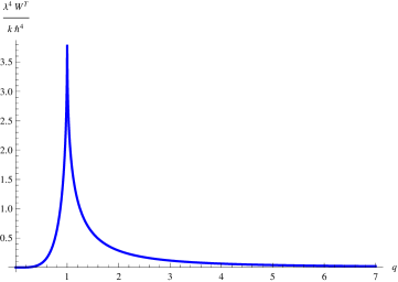
Figure 1: The form of potential after polymerization with $\lambda=1$ in $q$ polarization. Note that for simplicity we have plotted $\frac{W^{T}}{(k\hbar^{4}/\lambda^{4})}=\left(\sqrt{|q-1|}-\sqrt{|q+1|}\right)^{4}$, a continuous graph, while it actually should be a discrete one. The maximum is finite and here is equal to $4$.

One solution to both of the above problems (both functional differentiability of the action and/or its finiteness on classical solutions) comes from modifying the potential at infinity such that $q_{t\rightarrow\infty}<\infty$ and consequently $\delta q=0$ at the (time) boundary. This is the subject of the next section. In the remaining part of this section, we investigate the effects of polymerization on the Hamilton-Jacobi counterterm in $q$ polarization. To do this, we first derive the effective Euclidean Hamiltonian in $q$ polarization using the path integral method. This turns out to be (see Appendix C)

$$H_{\textrm{eff}}=\frac{2\hbar^{2}}{m\lambda^{2}}\sin^{2}\left(\frac{\lambda p}{2\hbar}\right)-W^{T}=\frac{2\hbar^{2}}{m\lambda^{2}}\sin^{2}\left(\frac{\lambda p}{2\hbar}\right)-\frac{k\hbar^{4}}{\lambda^{4}}\left(\sqrt{|q-\lambda|}-\sqrt{|q+\lambda|}\right)^{4},$$ (47)

where $W^{T}$ is the continuous counterpart of the potential derived using Thiemann’s regularization. A note about some subtleties is in order here: we could not directly argue that the form of the effective Hamiltonian will be (47) based on the form of the potential in (45). This is so because if one computes the action of the full quantum Hamiltonian on $|q_{n}\rangle$ states, one gets the above effective potential but with discrete $q_{n}$, and also the kinetic term will not be $\frac{2\hbar^{2}}{m\lambda^{2}}\sin^{2}\left(\frac{\lambda p}{2\hbar}\right)$ anymore since this is the form of the kinetic term when it acts on $|p\rangle$ states and not the $|q_{n}\rangle$ ones. On the other hand, if we use the $|p\rangle$ basis for the action of the full quantum Hamiltonian, we would not get the effective potential in (47). In the first case (acting $\hat{H}$ on $|q_{n}\rangle$), one will get an additional $\int dp$ in the kinetic term (and also the potential will be discrete), while in the second case (acting $\hat{H}$ on $|p\rangle$), there will be a $\sum_{n}$ in the potential term. The way to overcome these problems and get the effective action (47) is to use the path integral formulation and not something like $H_{\textrm{eff}}=\langle q_{n}|H|q_{n}\rangle$. What makes the path integral method useful is that one can bring the extra $\sum_{n}$ out of the exponential of the action and turn it into an integral that appears in the measure of the path integral (see Appendix C for more details).

To find the explicit form of the polymer $G_{\textrm{poly}}$ for this effective Hamiltonian, we need to solve (17). Considering the above Hamiltonian and noting that $p=\frac{\partial G_{\textrm{poly}}}{\partial q}$, Eq. (17) becomes

$$\frac{2\hbar^{2}}{m\lambda^{2}}\sin^{2}\left(\frac{\lambda}{2\hbar}\frac{\partial G_{\textrm{poly}}}{\partial q}\right)-\frac{k\hbar^{4}}{\lambda^{4}}\left(\sqrt{|q-\lambda|}-\sqrt{|q+\lambda|}\right)^{4}+\frac{\partial G_{\textrm{poly}}}{\partial t}=0.$$ (48)

Again since the Hamiltonian does not depend explicitly on $t$, Eq. (17) implies that the derivative $\nicefrac{{\partial G_{\textrm{poly}}}}{{\partial t}}$ must be a constant $H=E$, and an additive separation of variables in $G_{\textrm{poly}}$ can be performed

$$G_{\textrm{poly}}(q,E,t)=\Omega(q,E)-Et.$$ (49)

This turns (48) into

$$\frac{2\hbar^{2}}{m\lambda^{2}}\sin^{2}\left(\frac{\lambda}{2\hbar}\frac{\partial\Omega}{\partial q}\right)-\frac{k\hbar^{4}}{\lambda^{4}}\left(\sqrt{|q-\lambda|}-\sqrt{|q+\lambda|}\right)^{4}-E=0$$ (50)

or

$$\frac{\partial\Omega}{\partial q}=\frac{2}{\lambda}\sin^{-1}\left(\sqrt{\frac{m\lambda^{2}}{2\hbar^{2}}E+\frac{mk\hbar^{2}}{2\lambda^{2}}\left(\sqrt{|q-\lambda|}-\sqrt{|q+\lambda|}\right)^{4}}\right).$$ (51)

As clearly seen from this, finding $\Omega$ in this case is much more involved due to the presence of $\sin^{-1}\sqrt{\cdots}$. A way around this difficulty is to use a perturbative expansion of the right hand side of the above, around $\nicefrac{{\lambda}}{{q}}=0$. This yields

$$\frac{\partial\Omega}{\partial q}=\frac{\sqrt{2}\sqrt{m}\sqrt{Eq^{2}+k}}{q}+\frac{\lambda^{2}}{12\hbar^{2}q^{3}}\left(\sqrt{2}m^{\nicefrac{{3}}{{2}}}\left(Eq^{2}+k\right)^{\nicefrac{{3}}{{2}}}+\frac{3k\hbar^{2}\sqrt{2}\sqrt{m}}{\sqrt{Eq^{2}+k}}\right)+\mathcal{O}\left(\frac{\lambda^{4}}{\hbar^{4}}\right)$$ (52)

The leading continuum order in (52), in which $\lambda=0$, matches exactly the corresponding classical counterpart in (22). Integrating (52) and then substituting the result into (49) yields

$$G_{\textrm{poly}}= -Et+\sqrt{2}\sqrt{m}\sqrt{Eq^{2}+k}+\sqrt{2}\sqrt{mk}\tan^{-1}\left(\sqrt{\frac{k}{Eq^{2}+k}}\right)$$ (53)

$$+\frac{\lambda^{2}}{\hbar^{2}}\left[\frac{\sqrt{2}\sqrt{m}\sqrt{Eq^{2}+k}}{24q^{2}}\left(m\left(2Eq^{2}-k\right)-3\hbar^{2}\right)+\frac{\sqrt{2}\sqrt{m}}{8\sqrt{k}}E(+mk+\hbar^{2})\tan^{-1}\left(\sqrt{\frac{k}{Eq^{2}+k}}\right)\right]+\mathcal{O}\left(\frac{\lambda^{4}}{\hbar^{4}}\right).$$ (54)

Again we see that the purely classical term with $\lambda=0$ matches exactly to the classical Hamilton’s principal function (23) while there are also several types of corrections due to polymer quantization.

Since the classical part of the polymerized $G_{\textrm{poly}}$ in (54) is exactly the same as the classical nonpolymerized case, and since we have seen that with purely classical $G$, the action is functionally differentiable and its value on classical solutions is finite, we conclude that the polymerized improved action $\Gamma_{\textrm{poly}}[q_{cl}]$ with the above counterterm has also the same nice properties and thus makes it possible to proceed with the saddle point approximation if desired. But in addition to that, the counterterm (54) has additional terms proportional to the powers of “quantum lattice parameter” $\lambda$. So, it is reasonable to expect that this, together with the change of the form of the bulk action due to polymer quantization, will change the thermodynamical properties of the system in case of, e.g., a black hole, and therefore it is interesting to see what are the implications of such semiclassical polymer modifications. Next we consider the other polymer polarization.

IV The polymer model with discrete momentum

In this section we consider the $p$ polarization in which

$$\hat{U}_{\mu}|p_{n}\rangle= |p_{n}-\mu\rangle,$$ (55)

$$\hat{p}|p_{n}\rangle= p_{n}|p_{n}\rangle,$$ (56)

$$\hat{U}_{\mu}|q\rangle= e^{\frac{i}{\hbar}\mu q}|q\rangle,$$ (57)

$$\hat{p}|q\rangle= -\frac{\hbar}{i}\partial_{q}|q\rangle.$$ (58)

The representation of the kinetic term in (41) in this polarization is very simple; in fact it is just $\frac{\hat{p}^{2}}{2m}$. The problem here is how to represent the potential. It is not clear how Thiemann’s regularization can be used in this case. The reason is that generally this regularization is used to represent a variable that is discrete and not bounded. In the present case though we have to define a replacement for the inverse of $\hat{q}$; a problematic task since even $\hat{q}$ is not well defined on ${\cal{H}}_{p_{0}}$but only $\hat{U}_{\mu}$. Even more, we may consider finding functions $F(U_{\mu})$ and $G(p)$ such that classically

$$\frac{1}{q^{n}}=\left\{F\left(U_{\mu}\right),G(p)\right\}^{m},\,\,\,\,\,\,\,\,\,\,\,\,\,\,n,m>0,$$ (59)

so that $F(U_{\mu})$ and $G(p)$ admit a simple representation on Hilbert space. The first part, i.e., finding classical functions $F(U_{\mu})$ and $G(p)$ fulfilling (59) may not be very hard, and several options may be available such as

$$\frac{2}{\sqrt{\mu}}\left\{\sqrt{\big{|}-i\ln\left(U_{\mu}\right)\big{|}},p\right\}=\frac{2}{\sqrt{\mu}}\left\{\sqrt{\mu}\sqrt{\big{|}q\big{|}},p\right\}=\frac{1}{\sqrt{|q|}}.$$ (60)

However, the second part, the ability to represent the functions $F(U_{\mu})$ and $G(p)$ on Hilbert space, is the hard part as can be seen from the above example. Presently we have not found satisfactory functions that can be represented on $\mathcal{H}_{\textrm{poly}}$ for which Thiemann’s regularization can be done. In spite of this difficulty it is still possible to introduce a formal inverse squared position operator in this polarization and hence its semiclassical approximation.

We saw in the previous subsection that a solution to both issues of functional differentiability and finiteness of the action is likely to come from bounding $q$ to finite values, and this may result from modifying the potential term in $H_{E}$. Considering this, we can argue that since in this polarization, $q$ is bounded, a representation $\hat{W}(\hat{U}_{\mu})$ is expected to lead to a bounded potential and thus would eliminate the need to add a Hamilton-Jacobi boundary counterterm to the action to enable one to make a well-defined saddle point approximation. Now we provide a scheme that shows how the polymer quantization will change the action in such a way that no counterterm is needed to have a well-defined saddle point approximation.

Our proposed scheme for the effective potential is based on the observation that $q^{2}$ in this polarization gets replaced by an operator that is represented as (see Appendix (B))

$$q^{2}\rightarrow\widehat{q_{\mu}^{2}}=\frac{\hbar^{2}}{\mu^{2}}\left(2-\hat{U}_{\mu}-\hat{U}_{-\mu}\right).$$ (61)

Its action on a $|q\rangle$ basis is

$$\frac{\hbar^{2}}{\mu^{2}}\left(2-\hat{U}_{\mu}-\hat{U}_{-\mu}\right)|q\rangle= \frac{4\hbar^{2}}{\mu^{2}}\sin^{2}\left(\frac{\mu q}{2\hbar}\right)|q\rangle.$$ (62)

This is computed using (57) (see Appendix (B)). Based on this, our proposed replacement of the inverse squared operator is

$$\widehat{\frac{1}{q_{\mu}^{2}}}|q\rangle=\frac{\mu^{2}}{4\hbar^{2}}\csc^{2}\left(\frac{\mu q}{2\hbar}\right)|q\rangle.$$ (63)

Using path integral formulation, the effective action turns out to be (Appendix C)

$$S_{\textrm{eff}}=\int dt\left[p\dot{q}-\left(\frac{p^{2}}{2m}-\frac{\mu^{2}k}{4\hbar^{2}}\csc^{2}\left(\frac{\mu q}{2\hbar}\right)\right)\right].$$ (64)

Eq. (64) suggests that the effective form of the classical potential $W(q)=\frac{k}{q^{2}}$ in this scheme has an effective form

$$W^{h}=\frac{\mu^{2}k}{4\hbar^{2}}\csc^{2}\left(\frac{\mu q}{2\hbar}\right).$$ (65)

Note that here also there are subtleties similar to those explained in the previous section related to the important role of the path integral method to derive (64). For example, acting quantum Hamiltonian on $|q\rangle$ yields the above effective potential while the kinetic term will not be $\nicefrac{{p^{2}}}{{2m}}$ anymore since this is the form of the kinetic term when it acts on $|p\rangle$ not on $|q\rangle$ . Furthermore, since in this polarization our momentum states are actually discrete, i.e., $|p_{n}\rangle$, $p_{n}=n\mu,n\in\mathbb{Z}$, even if we act the kinetic term on them instead of $|q\rangle$, we will get a discrete result and not a continuous one. Thus again the path integral method saves the day and makes it possible to get rid of the additional $\sum_{n}$ and the discreteness of the momentum in the effective action. Details are explained in Appendix C.

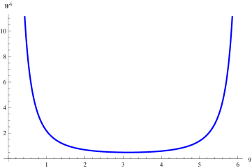
Figure 2: The form of potential $W^{h}$ for our model with $\mu=1$.

The plot of the potential (65) is shown in Fig. 2. Obviously the potential is still singular at the origin, $q=0$. But the good news is that the position is bounded at the time boundary, i.e., $q_{cl}(t\rightarrow\infty)<\infty$. This means that since now $q$ is finite at the boundary, $\delta q=0$ on the boundary, and thus the action is welldefined for a saddle point approximation without the need to add any other terms, such as the Hamilton-Jacobi counterterm. This polarization, like the previous one, will also most probably lead to modifications to the thermodynamics of the system due to the modification of the bulk action due to polymer quantization as well as the absence of any counterterm. This is particularly interesting if the system under study is a black hole.

V Discussion

In this work we have studied the issue of ill-defined saddle point semiclassical approximation that occurs for some systems including dilatonic black holes and some mathematically analog mechanical models. This problem arises due to the fact that the action is not functionally differentiable for all the variations of the fields, compatible with the boundary and falloff conditions and even if so, the value of the action on classical solutions does not remain finite for all of these conditions. This issue is rather important since one of the main methods of deriving thermodynamical properties of such models is through the saddle point approximation to the path integral that can also be interpreted as the partition function of the system. The common solution to this problem is to add a boundary counterterm to the action which is a solution to the corresponding Hamilton-Jacobi equation. A very interesting observation is that only with this term can one get the correct thermodynamics for certain black holes.

We undertake to seek an alternative method to attack this issue which is through polymer quantization of the model. The effects of polymerization may lead to two outcomes: either it will spare us altogether from adding any additional term to the action and the action is already well defined for saddle point approximation after polymer modifications, or it may not remove the necessity of adding a counterterm, but it will modify it. In both cases, it is very likely that the process of polymer quantization will change the thermodynamics, either due to the fact the counterterm is not necessary or because it will be modified.

In this work we restrict our study to a simpler analog model featuring the aforementioned issues. This helps us see the effects, problems, and results of this method more clearly and provides interesting insights about the procedure. The analog model we study is a single particle in an inverse square potential.

We first show how this system is modified under different polarizations of polymer quantization. It turns out that in the polarization where $q$ is discrete, we still will need to add the Hamilton-Jacobi counterterm to the action, but the advantage is that the potential can be rather easily represented on a Hilbert space using Thiemann’s regularization (Thiemann, 1998b). This is the case in which the Hamilton-Jacobi counterterm is modified by polymerization. We then proceed to compute the effective action and thus derive the effective Hamiltonian using path integral formulation. Then we derive the associated Hamilton-Jacobi counterterm and show that the classical terms of the polymerized case match exactly the nonpolymerized case while there are corrections to this counterterm that come from the polymer quantization. This supports our claim that polymer quantization will change the thermodynamics of the system due to the polymer modifications of the bulk action and the Hamilton-Jacobi counterterm.

On the other hand, in the polarization where $p$ is discrete, we argue that in general there should be no need to add a counterterm to the action since the variable $q$ is bounded due to polymer effects; thus the action remains functionally differentiable and finite on classical solutions in accordance with all the allowed variations. However, since the representation of the potential in this case is not so straightforward and could not be done here, in order to get concrete results and calculations, we proposed an effective form that replaces the classical potential $W=\frac{1}{q^{2}}$ based on the analysis of the polymer operator $\widehat{q^{2}_{\mu}}$. Using this, we show that the effective action is indeed finite evaluated on the effective solution and is functionally differentiable without the need to add a counterterm. This means that due to the effects of polymer quantization in $p$ polarization, the system is already well defined for saddle point approximation.

Further developments along the lines of the present work include the following. It is pretty evident that a similar analysis for the case of polymer black hole systems may lead to the change of thermodynamics due to polymer modifications of the bulk action. It will be interesting to check whether any counterterm is required in such a case. Also, recently, much work has been done to unveil singularity avoidance in loop quantum cosmology (Ashtekar et al., 2010a) as well as in black holes (Böhmer and Vandersloot, 2007; Corichi and Singh, 2015; Chiou, 2008) by alluding to effective models like the ones we have studied in the present work; hence it would be interesting to explore possible physical consequences for a semiclassical approximation of these systems using the path integral framework.

Appendix A Proof of (39) and (57)

Let us consider the polarization $(\hat{q},\hat{V}_{\lambda})$ where eigenvalues of the operator $\hat{q}$ are discrete. We would like to derive (39) from (36) and (37). Using the completeness relation

$$1=\frac{\lambda}{2\pi\hbar}\int_{-\nicefrac{{\pi\hbar}}{{\lambda}}}^{\nicefrac{{\pi\hbar}}{{\lambda}}}dp|p\rangle\langle p|$$ (66)

and the form of

$$\langle q_{n}|p\rangle=\sqrt{\frac{\lambda}{2\pi\hbar}}e^{\frac{ip_{n}q}{\hbar}}$$ (67)

one can write

$$\hat{V}_{\lambda}|p\rangle= \sum_{n=-\infty}^{\infty}\hat{V}_{\lambda}|q_{n}\rangle\langle q_{n}|p\rangle$$

$$= \frac{\lambda}{2\pi}\int_{-\nicefrac{{\pi}}{{\lambda}}}^{\nicefrac{{\pi}}{{\lambda}}}dp^{\prime}\sum_{n=-\infty}^{\infty}|p^{\prime}\rangle\langle p^{\prime}|q_{n}-\lambda\rangle\sqrt{\frac{\lambda}{2\pi\hbar}}e^{\frac{i}{\hbar}pq_{n}}$$

$$= \frac{\lambda}{2\pi}\int_{-\nicefrac{{\pi}}{{\lambda}}}^{\nicefrac{{\pi}}{{\lambda}}}dp^{\prime}\sum_{n=-\infty}^{\infty}|p^{\prime}\rangle e^{-\frac{i}{\hbar}p^{\prime}q_{n}}e^{\frac{i}{\hbar}p^{\prime}\lambda}e^{\frac{i}{\hbar}pq_{n}}$$

$$= \lambda\int_{-\nicefrac{{\pi}}{{\lambda}}}^{\nicefrac{{\pi}}{{\lambda}}}dp^{\prime}\lim_{j\rightarrow\infty}\underbrace{\left[\frac{1}{2\pi}\sum_{n=-j}^{j}e^{\frac{i}{\hbar}q_{n}(p-p^{\prime})}\right]}_{\delta_{n}(p-p^{\prime})}e^{\frac{i}{\hbar}p^{\prime}\lambda}|p^{\prime}\rangle,$$ (68)

where $\delta_{n}(p-p^{\prime})$ is a Dirac delta sequence and the limit will make it into a formal Dirac delta series representation $\delta(p-p^{\prime})$. Using the above and the fact that for a function $f(p)$ with a period $\nicefrac{{2\pi}}{{\lambda}}$ one can write

$$\int_{-\nicefrac{{\pi}}{{\lambda}}}^{\nicefrac{{\pi}}{{\lambda}}}dp^{\prime}\delta(p-p^{\prime})f(p^{\prime})=\frac{1}{\lambda}f(p),$$ (69)

we finally arrive at

$$\hat{V}_{\lambda}|p\rangle= e^{\frac{i}{\hbar}p\lambda}|p\rangle.$$ (70)

Using the same lines of argument but now in the polarization $(\hat{U}_{\mu},\hat{p})$ where eigenvalues of the operator $\hat{p}$ are discrete, one can derive (57) from (55) and (56).

Appendix B Action of $\widehat{q_{\mu}^{2}}|q\rangle$ and $\widehat{p_{\lambda}^{2}}|p\rangle$

Let us choose one of the polarizations, say the one in which $p$ is discrete. Since as mentioned before, the $\hat{q}$ operator does not exist in this polarization, we first need to construct an analog of the $q^{2}$ operator that we call $\widehat{q_{\mu}^{2}}$ and then find its action on the desired basis. To do this, we note that since classically $U_{\mu}=e^{\nicefrac{{i\mu q}}{{\hbar}}}$, then one can write

$$e^{\frac{i\mu q}{\hbar}}+e^{-\frac{i\mu q}{\hbar}}\approx 2-\frac{\mu^{2}q^{2}}{\hbar^{2}},\hskip 28.45274ptq\ll\frac{\hbar}{\mu}.$$ (71)

Using this, one can isolate $q^{2}$ and represent its singular counterpart $\widehat{q_{\mu}^{2}}$ (singular here means the limit $\mu\rightarrow 0$ does not exist) on the Hilbert space as

$$\widehat{q_{\mu}^{2}}=\frac{\hbar^{2}}{\mu^{2}}\left(2-\hat{U}_{\mu}-\hat{U}_{-\mu}\right),$$ (72)

and using the results of Appendix A or equivalently using (57), one can write

$$\frac{\hbar^{2}}{\mu^{2}}\left(2-\hat{U}_{\mu}-\hat{U}_{-\mu}\right)|q\rangle= \frac{\hbar^{2}}{\mu^{2}}\left(2-e^{\frac{i}{\hbar}\mu q}-e^{-\frac{i}{\hbar}\mu q}\right)|q\rangle$$ (73)

$$= \frac{\hbar^{2}}{\mu^{2}}\left(2-2\cos\left(\frac{\mu q}{\hbar}\right)\right)|q\rangle$$ (74)

$$= \frac{4\hbar^{2}}{\mu^{2}}\left(\sin^{2}\left(\frac{\mu q}{2\hbar}\right)\right)|q\rangle.$$ (75)

So we conclude that

$$\widehat{q_{\mu}^{2}}|q\rangle=\frac{4\hbar^{2}}{\mu^{2}}\left(\sin^{2}\left(\frac{\mu q}{2\hbar}\right)\right)|q\rangle.$$ (76)

On the other hand, if we choose to work in the polarizations in which $q$ is discrete, the operator $\widehat{p_{\lambda}^{2}}$ can be defined and represented using the same method, i.e.,

$$\widehat{p_{\lambda}^{2}}=\frac{\hbar^{2}}{\lambda^{2}}\left(2-\hat{V}_{\lambda}-\hat{V}_{-\lambda}\right).$$ (77)

Its action on the $|p\rangle$ basis can then be computed in the same manner as above for $\widehat{q_{\mu}^{2}}$, and by applying the results of Appendix A or equivalently Eq. (39) one gets

$$\widehat{p_{\lambda}^{2}}|p\rangle=\frac{4\hbar^{2}}{\lambda^{2}}\left(\sin^{2}\left(\frac{\lambda p}{2\hbar}\right)\right)|p\rangle.$$ (78)

Appendix C Effective polymerized actions

In this section we show how to obtain the effective action of the models described in Secs. III and IV. The calculations are done in Newtonian form but changing to the Euclidean form is straightforward. In steps that are different for each polarization, we will make comments and make clear what equation corresponds to which polarization. The transition amplitude in each case is given by

$$\langle q_{f},t_{f}\mid q_{i},t_{i}\rangle= \lim_{N\rightarrow\infty}\left(\prod_{n=1}^{N-1}\sum_{n}\right)\left(\prod_{n=1}^{N}\langle q_{n},t_{n}\mid q_{n-1},t_{n-1}\rangle\right),\,\,\,\,\,\,\,\,\,\,\,\,\,\,\,\,\,\,\,\,\,\,\,\,\,\,\,(\textrm{Discrete }q),$$ (79)

$$\langle q_{f},t_{f}\mid q_{i},t_{i}\rangle= \lim_{N\rightarrow\infty}\left(\prod_{n=1}^{N-1}\int_{-\frac{\pi\hbar}{\mu}}^{\frac{\pi\hbar}{\mu}}dq_{n}\right)\left(\prod_{n=1}^{N}\langle q_{n},t_{n}\mid q_{n-1},t_{n-1}\rangle\right),\,\,\,\,\,\,\,\,\,\,\,\,\,\,\,\,\,\,\,\,\,\,\,\,\,\,\,(\textrm{Discrete }p).$$ (80)

where in the first equation, we have a sum over polymer lattice $q$ points due to discreteness of $q$ and in the second equation, the limits of the integral reflect the bounds on the continuous variable $q$. Note that in the first equation, the subscript is due to the genuine polymer lattice discreteness of $q$, while in the second one, it is due to partitioning of the path integral. The amplitude above is then divided into partitions for which we have

$$\langle q_{n},t_{n}\mid q_{n-1},t_{n-1}\rangle= \langle q_{n}\mid e^{-\frac{i\epsilon}{\hbar}\hat{H}_{\textrm{poly}}}\mid q_{n-1}\rangle$$

$$\approx \langle q_{n}\mid 1-\frac{i\epsilon}{\hbar}\hat{H}_{\textrm{poly}}\mid q_{n-1}\rangle$$

$$= \langle q_{n}\mid q_{n-1}\rangle-\frac{i\epsilon}{\hbar}\langle q_{n}\mid\frac{\hbar^{2}}{2m}\left(\frac{2-\hat{V}_{\lambda}-\hat{V}_{-\lambda}}{\lambda^{2}}\right)\mid q_{n-1}\rangle-\frac{i\epsilon}{\hbar}\langle q_{n}\mid\hat{W}\mid q_{n-1}\rangle,$$ (81)

where $\hat{H}_{\textrm{poly}}$ is the polymer quantum Hamiltonian operator and we have used (77) for the representation of the kinetic term. $\hat{W}$ is the potential operator that can be represented by Thiemann’s regularization as in (44) in case $q$ is discrete or can be the potential proposed in Sec. IV when $p$ is discrete. We then insert one of the following identities:

$$1= \sum_{n}|p_{n}\rangle\langle p_{n}|,\,\,\,\,\,\,\,\,\,\,\,\,\,\,\,\,\,\,\,\,\,\,\,\,\,\,\,(\textrm{Discrete }p),$$ (82)

$$1= \frac{\lambda}{2\pi\hbar}\int_{-\frac{\pi\hbar}{\lambda}}^{\frac{\pi\hbar}{\lambda}}dp_{n}|p_{n}\rangle\langle p_{n}|,\,\,\,\,\,\,\,\,\,\,\,\,\,\,\,\,\,\,\,\,\,\,\,\,\,\,\,(\textrm{Discrete }q),$$ (83)

in front of the kinetic and potential terms in (81), corresponding to the polarization we are working in, to obtain either

$$\langle q_{n},t_{n}\mid q_{n-1},t_{n-1}\rangle\approx\frac{\lambda}{2\pi\hbar}\int_{-\frac{\pi\hbar}{\lambda}}^{\frac{\pi\hbar}{\lambda}}dp_{n}\langle q_{n}\mid p_{n}\rangle\langle p_{n}\mid q_{n-1}\rangle\left[1-\frac{i\epsilon}{\hbar}\left(\frac{2\hbar^{2}}{m\lambda^{2}}\sin^{2}\left(\frac{\lambda p}{2\hbar}\right)+W_{n}^{T}\right)\right]\,\,\,\,\,\,\,\,\,(\textrm{Discrete }q)$$ (84)

or

$$\langle q_{n},t_{n}\mid q_{n-1},t_{n-1}\rangle\approx \sum_{n}\langle q_{n}\mid p_{n}\rangle\langle p_{n}\mid q_{n-1}\rangle\left[1-\frac{i\epsilon}{\hbar}\left(\frac{p_{n}^{2}}{2m}+W_{n}^{h}\right)\right]\,\,\,\,\,\,\,\,\,\,\,\,\,\,\,\,\,\,\,\,\,\,\,\,\,\,\,(\textrm{Discrete }p).$$ (85)

Here

$$W_{n}^{T}= \frac{k\hbar^{4}}{\lambda^{4}}\left(\sqrt{|q_{n}-\lambda|}-\sqrt{|q_{n}+\lambda|}\right)^{4},$$ (86)

$$W_{n}^{h}= \frac{\mu^{2}k}{4\hbar^{2}}\csc^{2}\left(\frac{\mu q_{n}}{2\hbar}\right)$$ (87)

are Thiemann-regularized and heuristic polymer potentials, respectively. Note that again there are two types of subscripts associated with two types of discreteness. One is related to partitioning the full transition amplitude [as in (87)], and the other is related to the genuine polymer lattice discretization [as in (86)]. Using

$$\langle p\mid q_{n}\rangle= \sqrt{\frac{\lambda}{2\pi\hbar}}e^{-\frac{ipq_{n}}{\hbar}}\,\,\,\,\,\,\,\,\,\,\,\,\,\,\,\,\,\,\,\,\,\,\,\,\,\,\,(\textrm{Discrete }q),$$ (88)

$$\langle p_{n}\mid q\rangle= \sqrt{\frac{\mu}{2\pi\hbar}}e^{-\frac{ip_{n}q}{\hbar}}\,\,\,\,\,\,\,\,\,\,\,\,\,\,\,\,\,\,\,\,\,\,\,\,\,\,\,(\textrm{Discrete }p),$$ (89)

and also the full expansion of the exponential, one gets for the above partition transition amplitudes

$$\langle q_{n},t_{n}\mid q_{n-1},t_{n-1}\rangle= \left(\frac{\lambda}{2\pi\hbar}\right)^{2}\int_{-\frac{\pi\hbar}{\lambda}}^{\frac{\pi\hbar}{\lambda}}dp_{n}e^{\frac{i\epsilon}{\hbar}\left[p_{n}\frac{(q_{n}-q_{n-1})}{\epsilon}-\left(\frac{2\hbar^{2}}{m\lambda^{2}}\sin^{2}\left(\frac{\lambda p}{2\hbar}\right)+W_{n}^{T}\right)\right]}\,\,\,\,\,\,\,\,\,\,\,\,\,\,\,\,\,\,\,\,\,\,\,\,\,\,\,(\textrm{Discrete }q),$$ (90)

$$\langle q_{n},t_{n}\mid q_{n-1},t_{n-1}\rangle= \frac{\mu}{2\pi\hbar}\sum_{n}e^{\frac{i\epsilon}{\hbar}\left[p_{n}\frac{q_{n}-q_{n-1}}{\epsilon}-\left(\frac{p_{n}^{2}}{2m}+W_{n}^{h}\right)\right]}\,\,\,\,\,\,\,\,\,\,\,\,\,\,\,\,\,\,\,\,\,\,\,\,\,\,\,(\textrm{Discrete }p).$$ (91)

Using these in corresponding full transition amplitudes (79) and (80) yields

$$\langle q_{f},t_{f}|q_{i},t_{i}\rangle= \lim_{N\rightarrow\infty,\epsilon\rightarrow 0}\left(\prod_{n=1}^{N-1}\sum_{n}\right)\left(\left(\frac{\lambda}{2\pi\hbar}\right)^{2}\prod_{n=1}^{N}\int_{-\frac{\pi\hbar}{\lambda}}^{\frac{\pi\hbar}{\lambda}}dp_{n}\right)e^{\sum_{n=1}^{N}\frac{i\epsilon}{\hbar}\left[p_{n}\frac{(q_{n}-q_{n-1})}{\epsilon}-\left(\frac{2\hbar^{2}}{m\lambda^{2}}\sin^{2}\left(\frac{\lambda p}{2\hbar}\right)+W_{n}^{T}\right)\right]}\,\,\,\,(\textrm{Discrete }q),$$ (92)

$$\langle q_{f},t_{f}|q_{i},t_{i}\rangle= \lim_{N\rightarrow\infty,\epsilon\rightarrow 0}\left(\prod_{n=1}^{N-1}\int_{-\frac{\pi\hbar}{\mu}}^{\frac{\pi\hbar}{\mu}}dq_{n}\right)\left(\frac{\mu}{2\pi\hbar}\prod_{n=1}^{N}\sum_{n}\right)e^{\sum_{n=1}^{N}\frac{i\epsilon}{\hbar}\left[p_{n}\frac{q_{n}-q_{n-1}}{\epsilon}-\left(\frac{p_{n}^{2}}{2m}+W_{n}^{h}\right)\right]}\,\,\,\,\,\,\,\,\,\,\,\,\,(\textrm{Discrete }p).$$ (93)

In both cases above, we have a $\sum_{n}$ in front of the exponential while we should have an integral instead. In other words, if we wish to have a normal path integral, we need to pass from a discrete variable, say $q_{n}$, to the continuous one $q$ (and the same for $p_{n}$). To achieve this we use the identity (Ashtekar et al., 2010a)

$$\sum_{n}\int_{0}^{2\pi}dqf(q,p_{n})e^{ip_{n}q}=\int_{-\infty}^{\infty}dq\int_{-\infty}^{\infty}dpf(p,q)e^{iqp},$$ (94)

valid for $f(q,p)$ which are periodic in $q$, and a similar expression also holds for the case with discrete $p_{n}$. Let us consider first the expression (93). Using the above identity, one gets for (93)

$$\langle q_{f},t_{f}|q_{i},t_{i}\rangle=\lim_{N\rightarrow\infty,\epsilon\rightarrow 0}\left(\prod_{n=1}^{N-1}\int_{-\infty}^{\infty}dq_{n}\right)\left(\frac{\mu}{2\pi\hbar}\prod_{n=1}^{N}\int_{-\infty}^{\infty}dp\right)e^{\frac{i\epsilon}{\hbar}\sum_{n=1}^{N}\left[p_{n}\frac{q_{n}-q_{n-1}}{\epsilon}-\left(\frac{p_{n}^{2}}{2m}+W_{n}^{h}\right)\right]}\,\,\,\,\,\,\,\,\,(\textrm{Discrete }p),$$ (95)

which is the polymer Feynman formula. Taking the limits in (95) above yields

$$\langle q_{f},t_{f}|q_{i},t_{i}\rangle=\frac{\mu}{2\pi\hbar}\left(\prod_{n}\int_{-\infty}^{\infty}dq_{n}\right)\left(\prod_{n}\int_{-\infty}^{\infty}dp\right)e^{\frac{i}{\hbar}\int dt\left[p\dot{q}-\left(\frac{p^{2}}{2m}+W^{h}\right)\right]}\,\,\,\,\,\,\,\,\,\,\,\,\,\,\,\,\,\,\,\,\,\,\,\,\,\,\,(\textrm{Discrete }p),$$ (96)

where the effective action can be read off to be

$$S_{\textrm{eff}}=\int dt\left[p\dot{q}-H_{\textrm{eff}}\right]=\int dt\left[p\dot{q}-\left(\frac{p^{2}}{2m}+\frac{\mu^{2}k}{4\hbar^{2}}\csc^{2}\left(\frac{\mu q_{n}}{2\hbar}\right)\right)\right]\,\,\,\,\,\,\,\,\,\,\,\,\,\,\,\,\,\,\,\,\,\,\,\,\,\,\,(\textrm{Discrete }p).$$ (97)

The case with discrete $q$ is a bit more delicate because of the inherent discreteness that precludes the limit

$$\lim_{\epsilon\rightarrow 0}\left(p_{n}\frac{q_{n}-q_{n-1}}{\epsilon}\right)\rightarrow p\dot{q}.$$ (98)

To deal with this, one uses a method similar to Leibniz rule for discrete variables. One can rewrite the sum that appears in the kinetic term as

$$\sum_{n=1}^{N}p_{n}\frac{q_{n}-q_{n-1}}{\epsilon}= \frac{1}{\epsilon}\left(\sum_{n=1}^{N}p_{n}q_{n}-\sum_{n=1}^{N}p_{n}q_{n-1}\right)$$

$$= \frac{1}{\epsilon}\left(\sum_{n=1}^{N}p_{n}q_{n}-\sum_{m=0}^{N-1}p_{m+1}q_{m}\right)$$

$$= \frac{1}{\epsilon}\left(\sum_{n=1}^{N-1}p_{n}q_{n}-\sum_{n=1}^{N-1}p_{n+1}q_{n}+p_{N}q_{N}-p_{1}q_{0}\right)$$

$$= \frac{1}{\epsilon}\left(-\sum_{n=1}^{N-1}\left[\left(p_{n+1}-p_{n}\right)q_{n}\right]+p_{N}q_{N}-p_{1}q_{0}\right),$$ (99)

which is similar to expressing $p\dot{q}=-q\dot{p}+\dot{(pq)}$ where $\frac{1}{\epsilon}\left(p_{N}q_{N}-p_{1}q_{0}\right)$ plays the rule of the “boundary term” $(pq)\dot{\,}$ in a discrete sense. Using this, expression (92) becomes

$$\langle q_{f},t_{f}|q_{i},t_{i}\rangle= \lim_{N\rightarrow\infty,\epsilon\rightarrow 0}\left(\prod_{n=1}^{N-1}\sum_{n}\right)\left(\left(\frac{\lambda}{2\pi\hbar}\right)^{2}\prod_{n=1}^{N}\int_{-\frac{\pi\hbar}{\lambda}}^{\frac{\pi\hbar}{\lambda}}dp_{n}\right)\times$$

$$e^{\frac{i\epsilon}{\hbar}\left[\sum_{n=1}^{N-1}\left[\frac{-\left(p_{n+1}-p_{n}\right)q_{n}+p_{N}q_{N}-p_{1}q_{0}}{\epsilon}\right]-\sum_{n=1}^{N}\left(\frac{2\hbar^{2}}{m\lambda^{2}}\sin^{2}\left(\frac{\lambda p}{2\hbar}\right)+W_{n}^{T}\right)\right]}\,\,\,\,\,\,\,\,\,\,\,\,\,\,\,\,\,\,\,\,\,\,\,\,\,\,\,(\textrm{Discrete }q).$$ (100)

Now, we can take the limit such that the term $\lim_{\epsilon\rightarrow 0}\frac{-\left(p_{n+1}-p_{n}\right)q_{n}+p_{N}q_{N}-p_{1}q_{0}}{\epsilon}$ becomes $-q\dot{p}+\dot{(pq)}$, which in the continuous limit can be rewritten as $p\dot{q}$. Before taking this limit, we use an identity similar to (94) but for discrete $q$,

$$\sum_{n}\int_{0}^{2\pi}dpf(q_{n},p)e^{iq_{n}p}=\int_{-\infty}^{\infty}dq\int_{-\infty}^{\infty}dpf(p,q)e^{iqp},$$ (101)

to turn $\sum_{n}$ into an integral. Then by taking the limits, one gets

$$\langle q_{f},t_{f}|q_{i},t_{i}\rangle=\left(\frac{\lambda}{2\pi\hbar}\right)^{2}\left(\prod_{n}\int_{-\infty}^{\infty}dq_{n}\right)\left(\prod_{n}\int_{-\infty}^{\infty}dp_{n}\right)e^{\frac{i\epsilon}{\hbar}\left[p\dot{q}-\left(\frac{2\hbar^{2}}{m\lambda^{2}}\sin^{2}\left(\frac{\lambda p}{2\hbar}\right)+W^{T}\right)\right]}\,\,\,\,\,\,\,\,\,\,\,\,\,\,\,\,\,\,\,\,\,\,\,\,\,\,\,(\textrm{Discrete }q)$$ (102)

Note that the potential does not have a discrete subscript anymore since we turned $q_{n}$ into a continuous variable $q$ by using (101). Thus the effective action can be read off to be

$$S_{\textrm{eff}}=\int dt\left[p\dot{q}-H_{\textrm{eff}}\right]=\int dt\left[p\dot{q}-\left(\frac{2\hbar^{2}}{m\lambda^{2}}\sin^{2}\left(\frac{\lambda p}{2\hbar}\right)+\frac{k\hbar^{4}}{\lambda^{4}}\left(\sqrt{|q-\lambda|}-\sqrt{|q+\lambda|}\right)^{4}\right)\right]\,\,\,\,\,\,\,\,\,\,\,\,\,\,\,\,\,\,\,\,\,\,(\textrm{Discrete }q).$$ (103)

Appendix D Action of $\hat{H}_{E}$ in $(\hat{q},\hat{V}_{\lambda})$ polarization

D.1 In $|q_{n}\rangle$ basis

The action of the Hamiltonian (44) on the basis $|q_{n}\rangle$ in the polarization (36)-(39) can be computed as follows. The kinetic term acts like

$$\frac{\widehat{p_{\lambda}^{2}}}{2m}|q_{n}\rangle=\frac{\hbar^{2}}{2m}\left(\frac{2-\hat{V}_{\lambda}-\hat{V}_{-\lambda}}{\lambda^{2}}\right)|q_{n}\rangle=\frac{\hbar^{2}}{2m\lambda^{2}}\left(2|q_{n}\rangle-|q_{n}-\lambda\rangle-|q_{n}+\lambda\rangle\right),$$ (104)

where the operator $\widehat{p_{\lambda}^{2}}$ is defined in (77). The potential $\hat{W}$ in (44) has two terms for each of which we have

$$\frac{\hat{V}_{-\lambda}}{\lambda}\left[\widehat{\sqrt{|q|}},\hat{V}_{\lambda}\right]|q_{n}\rangle=\frac{1}{\lambda}\sqrt{|q_{n}-\lambda|}|q_{n}\rangle-\frac{1}{\lambda}\sqrt{|q_{n}|}|q_{n}\rangle$$ (105)

and

$$\left[\widehat{\sqrt{|q|}},\hat{V}_{\lambda}\right]\frac{\hat{V}_{-\lambda}}{\lambda}|q_{n}\rangle=\frac{1}{\lambda}\sqrt{|q_{n}|}|q_{n}\rangle-\frac{1}{\lambda}\sqrt{|q_{n}+\lambda|}|q_{n}\rangle.$$ (106)

Thus the full expression for the action of the potential in this basis becomes

$$\hat{W}|q\rangle=k\hbar^{4}\left(\frac{\hat{V}_{-\lambda}}{\lambda}\left[\widehat{\sqrt{|q|}},\hat{V}_{\lambda}\right]+\left[\widehat{\sqrt{|q|}},\hat{V}_{\lambda}\right]\frac{\hat{V}_{-\lambda}}{\lambda}\right)^{4}|q_{n}\rangle=\frac{k\hbar^{4}}{\lambda^{4}}\left(\sqrt{|q_{n}-\lambda|}-\sqrt{|q_{n}+\lambda|}\right)^{4}|q_{n}\rangle$$ (107)

D.2 In $|p\rangle$ basis

One can act the Hamiltonian (44) on basis $|p\rangle$ where

$$\hat{V}_{\lambda}|p\rangle=e^{\frac{i}{\hbar}\lambda p}|p\rangle.$$ (108)

Then the kinetic term in (44) turns out to be

$$\frac{\widehat{p_{\lambda}^{2}}}{2m}|p\rangle=\frac{\hbar^{2}}{2m}\left(\frac{2-\hat{V}_{\lambda}-\hat{V}_{-\lambda}}{\lambda^{2}}\right)|p\rangle= \frac{2\hbar^{2}}{m\lambda^{2}}\sin^{2}\left(\frac{\lambda p}{2\hbar}\right)|p\rangle$$ (109)

where we have used (77) and (78). To find the action of the potential term, we first note that

$$\hbar^{4}\left(\frac{\hat{V}_{-\lambda}}{\lambda}\left[\widehat{\sqrt{|q|}},\hat{V}_{\lambda}\right]+\left[\widehat{\sqrt{|q|}},\hat{V}_{\lambda}\right]\frac{\hat{V}_{-\lambda}}{\lambda}\right)^{4}|p\rangle= k\hbar^{4}\left(\frac{\hat{V}_{-\lambda}}{\lambda}\left[\widehat{\sqrt{|q|}},\hat{V}_{\lambda}\right]+\left[\widehat{\sqrt{|q|}},\hat{V}_{\lambda}\right]\frac{\hat{V}_{-\lambda}}{\lambda}\right)^{4}\sum_{n}|q_{n}\rangle\langle q_{n}|p\rangle.$$ (110)

Then using the results of the previous subsection, we get for the action of the potential in this case

$$k\hbar^{4}\left(\frac{\hat{V}_{-\lambda}}{\lambda}\left[\widehat{\sqrt{|q|}},\hat{V}_{\lambda}\right]+\left[\widehat{\sqrt{|q|}},\hat{V}_{\lambda}\right]\frac{\hat{V}_{-\lambda}}{\lambda}\right)^{4}|p\rangle=\frac{k\hbar^{4}}{\lambda^{4}}\sum_{n}\left(\sqrt{|q_{n}-\lambda|}-\sqrt{|q_{n}+\lambda|}\right)^{4}|q_{n}\rangle\langle q_{n}|p\rangle.$$ (111)

References

- Rovelli (2004) C. Rovelli, Quantum Gravity, 1st ed. (Cambridge University Press, 2004).
- Thiemann (2007) T. Thiemann, Modern Canonical Quantum General Relativity, 1st ed. (Cambridge University Press, 2007).
- Gambini and Pullin (2011) R. Gambini and J. Pullin, A First Course in Loop Quantum Gravity, 1st ed. (Oxford University Press, 2011).
- Bojowald (2011) M. Bojowald, Canonical Gravity and Applications: Cosmology, Black Holes and Quantum Gravity, 1st ed. (Cambridge University Press, 2011).
- Rovelli and Vidotto (2014) C. Rovelli and F. Vidotto, Covariant Loop Quantum gravity: An Elementary Introduction to Quantum Gravity and Spin Foam Theory, 1st ed. (Cambridge Monographs on Mathematical Physics, 2014).
- Bojowald (2001) M. Bojowald, “Absence of Singularity in Loop Quantum Cosmology,” Phys.Rev.Lett. 86, 5227–5230 (2001), arXiv:gr-qc/0102069 [gr-qc] .
- Ashtekar et al. (2006) A. Ashtekar, T. Pawlowski, and P. Singh, “Quantum nature of the big bang: Improved dynamics,” Phys.Rev. D74, 084003 (2006), arXiv:gr-qc/0607039 [gr-qc] .
- Thiemann (1998a) T. Thiemann, “QSD 5: Quantum gravity as the natural regulator of matter quantum field theories,” Class.Quant.Grav. 15, 1281–1314 (1998a), arXiv:gr-qc/9705019 [gr-qc] .
- Ashtekar et al. (1998) A. Ashtekar, J. Baez, A. Corichi, and K. Krasnov, “Quantum geometry and black hole entropy,” Phys.Rev.Lett. 80, 904–907 (1998), arXiv:gr-qc/9710007 [gr-qc] .
- Ashtekar et al. (2003) A. Ashtekar, S. Fairhurst, and J. L. Willis, “Quantum gravity, shadow states, and quantum mechanics,” Class.Quant.Grav. 20, 1031–1062 (2003), arXiv:gr-qc/0207106 [gr-qc] .
- Corichi et al. (2007a) A. Corichi, T. Vukasinac, and J. A. Zapata, “Hamiltonian and physical Hilbert space in polymer quantum mechanics,” Class.Quant.Grav. 24, 1495–1512 (2007a), arXiv:gr-qc/0610072 [gr-qc] .
- Corichi et al. (2007b) A. Corichi, T. Vukasinac, and J. A. Zapata, “Polymer Quantum Mechanics and its Continuum Limit,” Phys.Rev. D76, 044016 (2007b), arXiv:0704.0007 [gr-qc] .
- Flores-Gonzĺez et al. (2013) E. Flores-Gonzĺez, H. A. Morales-Técotl, and J. D. Reyes, “Propagators in Polymer Quantum Mechanics,” Annals Phys. 336, 394–412 (2013), arXiv:1302.1906 [math-ph] .
- Hossain et al. (2010) G. M. Hossain, V. Husain, and S. S. Seahra, “The Propagator in polymer quantum field theory,” Phys.Rev. D82, 124032 (2010), arXiv:1007.5500 [gr-qc] .
- García-Chung and Morales-Técotl (2014) A. A. García-Chung and H. A. Morales-Técotl, “Polymer Dirac field propagator: A model,” Phys.Rev. D89, 065014 (2014).
- Cumsille et al. (2015) P. Cumsille, C. M. Reyes, S. Ossandon, and C. Reyes, “Polymer quantization, stability and higher-order time derivative terms,” (2015), arXiv:1503.07153 [hep-th] .
- Husain and Winkler (2003) V. Husain and O. Winkler, “Particles, spinfoams and the Hamiltonian path integral,” Unpublished (2003).
- Ashtekar et al. (2009) A. Ashtekar, M. Campiglia, and A. Henderson, “Loop Quantum Cosmology and Spin Foams,” Phys.Lett. B681, 347–352 (2009), arXiv:0909.4221 [gr-qc] .
- Ashtekar et al. (2010a) A. Ashtekar, M. Campiglia, and A. Henderson, “Path Integrals and the WKB approximation in Loop Quantum Cosmology,” Phys.Rev. D82, 124043 (2010a), arXiv:1011.1024 [gr-qc] .
- Ashtekar et al. (2010b) A. Ashtekar, M. Campiglia, and A. Henderson, “Casting Loop Quantum Cosmology in the Spin Foam Paradigm,” Class.Quant.Grav. 27, 135020 (2010b), arXiv:1001.5147 [gr-qc] .
- Kajuri (2015) N. Kajuri, “Path integrals and lorentz violation in polymer quantized scalar fields,” (2015), arXiv:1406.7400 [gr-qc] .
- Parra and Vergara (2014) L. Parra and J. D. Vergara, “Polymer quantum mechanics some examples using path integrals,” AIP Conf.Proc. 1577, 269–280 (2014).
- Morales-Técotl et al. (2015) H. Morales-Técotl, S. Rastgoo, and J. C. Ruelas, “Path integral propagator of relativistic and non relativistic particles,” In preparation (2015).
- Regge and Teitelboim (1974) T. Regge and C. Teitelboim, “Role of surface integrals in the Hamiltonian formulation of general relativity,” Ann. Phys. 88, 286 (1974).
- Gibbons and Hawking (1977) G. W. Gibbons and S. W. Hawking, “Action integrals and partition functions in quantum gravity,” Phys. Rev. D15, 2752 (1977).
- Liebl et al. (1997) H. Liebl, D. V. Vassilevich, and S. Alexandrov, “Hawking radiation and masses in generalized dilaton theories,” Class. Quantum Grav. 14, 889 (1997).
- Papadimitriou and Skenderis (2005) I. Papadimitriou and K. Skenderis, “Thermodynamics of asymptotically locally ads spacetimes,” JHEP 08 (2005), 004, arXiv:hep-th/0505190 .
- McNees (2005) R. McNees, “A new boundary counterterm for asymptotically ads spacetimes,” (2005), arXiv:hep-th/0512297 .
- Mann and Marolf (2006) R. B. Mann and D. Marolf, “Holographic renormalization of asymptotically flat spacetimes,” Class. Quantum Grav. 23, 2927 (2006).
- Callan et al. (1992) C. G. Callan, S. B. Giddings, J. A. Harvey, and A. Strominger, “Evanescent black holes,” Phys. Rev. D45, R1005 (1992), arXiv:hep-th/9111056v1 .
- Grumiller and McNees (2007) D. Grumiller and R. McNees, “Thermodynamics of black holes in two (and higher) dimensions,” JHEP 04 (2007), 074, arXiv:hep-th/0703230 .
- York (1972) J. W. York, “Role of conformal three-geometry in the dynamics of gravitation,” Phys. Rev. Lett. 28, 1082 (1972).
- Husain et al. (2007) V. Husain, J. Louko, and O. Winkler, “Quantum gravity and the coulomb potential,” Phys. Rev. D 76, 084002 (2007).
- Kunstatter et al. (2009) Gabor Kunstatter, Jorma Louko, and Jonathan Ziprick, “Polymer quantization, singularity resolution and the 1/r**2 potential,” Phys.Rev. A79, 032104 (2009), arXiv:0809.5098 [gr-qc] .
- Grumiller (2007) D. Grumiller, “Path integral for half-binding potentials as quantum mechanical analog for black hole partition functions,” (2007), arXiv:0711.4115 [quant-ph] .
- Thiemann (1998b) T. Thiemann, “Quantum spin dynamics (qsd),” Class. Quantum. Grav. 15, 839–873 (1998b), arXiv:gr-qc/9606089 .
- Böhmer and Vandersloot (2007) C. G. Böhmer and K. Vandersloot, “Loop quantum dynamics of the schwarzschild interior,” Phys.Rev. D76, 104030 (2007).
- Corichi and Singh (2015) A. Corichi and P. Singh, “Loop quantization of the schwarzschild interior revisited,” (2015), arXiv:gr-qc/1506.08015 [gr-qc] .
- Chiou (2008) D. Chiou, “Phenomenological loop quantum geometry of the schwarzschild black hole,” Phys.Rev. D78, 064040 (2008).