Imaginary-time matrix product state impurity solver for dynamical mean-field theory

Abstract

We present a new impurity solver for dynamical mean-field theory based on imaginary-time evolution of matrix product states. This converges the self-consistency loop on the imaginary-frequency axis and obtains real-frequency information in a final real-time evolution. Relative to computations on the real-frequency axis, required bath sizes are much smaller and less entanglement is generated, so much larger systems can be studied. The power of the method is demonstrated by solutions of a three band model in the single and two-site dynamical mean-field approximation. Technical issues are discussed, including details of the method, efficiency as compared to other matrix product state based impurity solvers, bath construction and its relation to real-frequency computations and the analytic continuation problem of quantum Monte Carlo, the choice of basis in dynamical cluster approximation, and perspectives for off-diagonal hybridization functions.

I Introduction

Dynamical mean-field theory (DMFT) in its single-site Metzner and Vollhardt (1989); Georges and Kotliar (1992); Georges et al. (1996) and cluster Maier et al. (2005); Kotliar et al. (2006) variants is among the most widely employed computational techniques for solving quantum many-body problems. At the core of a numerical solution of DMFT is an impurity solver: an algorithm for solving a quantum impurity problem. The most prominent examples of impurity solvers are continuous time quantum Monte Carlo (CTQMC) (Rubtsov et al., 2005; Werner et al., 2006; Gull et al., 2011), exact diagonalization (ED) (Caffarel and Krauth, 1994; Capone et al., 2007; Liebsch and Ishida, 2012), the numerical renormalization group (NRG) (Bulla et al., 2008), and the density matrix renormalization group (DMRG) (García et al., 2004). While all methods have their strengths, key limitations mean that fundamentally important classes of problems have not yet been adequately addressed. Other recent suggestions for impurity solvers (Li and Tong, 2015; Wang et al., 2015; Arsenault et al., 2015; Schüler et al., 2015; Granath and Strand, 2012; Shinaoka et al., 2014) including in particular the computationally inexpensive density matrix embedding theory (DMET) (Knizia and Chan, 2012), are promising but have not been tested in detail.

CTQMC is widely employed but its application to situations involving low point symmetry, non-Hubbard interactions or multiple relevant orbitals is limited by the fermionic sign problem. Reaching low temperatures becomes highly computationally expensive while calculating real-frequency information requires analytical continuation, a numerically ill-posed procedure fraught with practical difficulties.

ED makes no assumption on the interaction and does not have a sign problem. It is limited by the size of the Hilbert space that can be studied, meaning in practice that it is restricted to a small number of correlated sites to which only a small number of bath sites can be attached. Recently, improvements have been achieved by considering only restricted subspaces of the Hilbert space (Lu et al., 2014; Zgid et al., 2012; Lin and Demkov, 2013a, b), but the size of problem remains a significant limitation.

NRG converges the DMFT loop on the real-frequency axis and very effectively obtains real-frequency information in the low frequency limit. Current applications have been to relatively small problems (the most recent achievement is a solution of the single-site DMFT approximation to a three-band model (Stadler et al., 2015)) and it remains to be seen how far the method can be extended.

DMRG (White, 1992) is a set of algorithms operating on the space of matrix product states (MPS) (Schollwöck, 2011). It has been found to be extremely powerful for the calculation of ground states of one-dimensional quantum systems (Schollwöck, 2005, 2011); it was very successfully extended to the calculation of spectral functions which, in contrast to NRG, it obtains with equal resolution across the spectrum, see e.g. (Holzner et al., 2011; Wolf et al., 2015). In pioneering work the method was applied as a DMFT solver by García, Hallberg, and Rozenberg (2004) and Nishimoto, Gebhard, and Jeckelmann (2004) with important further work done by these and other authors (Karski et al., 2005; Nishimoto et al., 2006; García et al., 2007; Karski et al., 2008; Peters, 2011; Ganahl et al., 2014a, b). However, the method has not been widely accepted, perhaps because high-quality data were presented only for the single-site approximation to the single-band Hubbard model. Recently the method was used to reliably solve a two-site DCA (Wolf et al., 2014a), and insights into the entanglement of the impurity problem made it even more powerful (Wolf et al., 2014b). In view of these advances, DMRG now is a candidate for a highly flexible low-cost impurity solver, which can in addition be efficiently employed in the non-equilibrium formulation of DMFT (Gramsch et al., 2013; Wolf et al., 2014b; Balzer et al., 2015).

This paper reformulates the DMRG method as an impurity solver for DMFT on the imaginary-time axis (Sec. II). As we will show, this strongly reduces entanglement and necessary bath sizes. The price to be paid is a reduced resolution on the real-frequency axis, which we study in detail by comparing with calculations that converge the DMFT loop on the real-frequency axis (Sec. III). The reformulation allows a much larger class of problems to be addressed, including some that are unreachable by other methods, due e.g. to the sign problem, the size of the correlated cluster or the number of bands. We illustrate this with calculations for three band models in the single-site and two-site DMFT approximation (Sec. IV). We append discussions of the optimization of typical DMFT Hamiltonians (Appendix A) and of the entanglement in different representations of the DCA including a discussion of off-diagonal hybridization functions (Appendix B).

II Method

II.1 Overview: Green’s functions in DMRG

The computational key challenge in DMFT is the computation of the full frequency dependence of the Green’s function of a quantum impurity model involving an essentially arbitrary bath. The “size” (number of correlated sites $L_{c}$) of the impurity model should be as large as possible and the kinds of interaction that can be treated should be as general as possible. The Green’s function is used in a self-consistency loop, which may require many iterations for convergence. The solution should be as inexpensive as feasible, and must run automatically, without need for manual optimization of parameters or procedures. In this subsection we present a qualitative discussion of the issues involved in computing the Green’s function using DMRG methods, to motivate the work described in detail below.

Within DMRG one computes Green’s functions by first representing the system ground state $|E_{0}\rangle$ as an MPS. One then generates a one electron (one hole) excitation $|\psi^{>}_{0}\rangle=d^{\dagger}|E_{0}\rangle$ $\left(|\psi^{<}_{0}\rangle=d|E_{0}\rangle\right)$ by applying a creation (annihilation) operator $d^{\dagger}$ ($d$) to $|E_{0}\rangle$. While the state $|\psi_{0}^{\gtrless}\rangle$ is at most as entangled as the ground state $|E_{0}\rangle$ (Wolf et al., 2015), in order to compute a Green’s function, one has to perform further operations on $|\psi_{0}^{\gtrless}\rangle$. These operations typically increase entanglement and by that the bond dimension of an MPS, which ultimately limits all computations.

Let us be more concrete and consider a general MPS of bond dimension $m$ for a system with $L$ sites and open boundary conditions. Defining $A^{\sigma_{i}},B^{\sigma_{i}}\in\mathbb{C}^{m\times m}$ for $i\neq 1,L$ and $A^{\sigma_{1}}\in\mathbb{C}^{1\times m}$, $B^{\sigma_{L}}\in\mathbb{C}^{m\times 1}$, where $\sigma_{i}\in\{0,\uparrow,\downarrow,\uparrow\downarrow\}$ labels a local basis state of the Hilbert space, any MPS can be represented as (Schollwöck, 2011)

$$|\psi_{\text{MPS}}\rangle=\!\!\sum_{\sigma_{1},...,\sigma_{L}}\!\!A^{\sigma_{1}}...\,A^{\sigma_{l}}SB^{\sigma_{l+1}}...\,B^{\sigma_{L}}|\sigma_{1},...,\sigma_{L}\rangle,$$ (1)

where $S=\text{diag}(s_{1},...,s_{m})$ is a diagonal matrix, and $A^{\sigma_{i}}$ are left-normalized and $B^{\sigma_{i}}$ are right-normalized, respectively:

$$\sum_{\sigma_{i}}A^{\sigma_{i}\dagger}A^{\sigma_{i}}=I,\qquad\sum_{\sigma_{i}}B^{\sigma_{i}}B^{\sigma_{i}\dagger}=I.$$ (2)

Here, $I$ are identity matrices. Left- and right-normalization make Eq. (1) the Schmidt decomposition of $|\psi_{\text{MPS}}\rangle$ that is associated with partitioning the system at bond $(l,l+1)$. The bond entanglement entropy for the associated reduced density matrix can therefore simply be read of from Eq. (1) (Schollwöck, 2011)

$$S_{(l,l+1)}^{\text{ent}}=\sum_{\nu=1}^{m}s_{\nu}^{2}\ln s_{\nu}^{2}.$$ (3)

When subsequently we refer to an entanglement growth associated with repeated operations on $|\psi_{\text{MPS}}\rangle$ this implies the need to adjust the bond dimension $m$ such that $|\psi_{\text{MPS}}\rangle$ still faithfully represents a physical state. If entanglement in the physical state becomes too large, we have to choose $m$ so large that computations with MPS become impractical.

Since the first suggestion for computing spectral functions within DMRG (Hallberg, 1995), the field has evolved by the important development of the correction vector method (Kühner and White, 1999; Jeckelmann, 2002). The subsequent understanding of the connection between DMRG and MPS (Schollwöck, 2011) opened the door to many further approaches to computing spectral and Green’s functions, in particular, time evolution and subsequent Fourier transform (White and Feiguin, 2004; White and Affleck, 2008), an improved Lanczos algorithm (Dargel et al., 2012), and the Chebyshev recursion (Holzner et al., 2011; Braun and Schmitteckert, 2014; Wolf et al., 2015). All of these are formulated for the calculation of spectral functions at $T=0$, as considered in the present paper, and came at much cheaper computational cost than the correction vector method (Holzner et al., 2011; Wolf et al., 2015). We note that for $T>0$, there are perspectives for even more powerful algorithms: it was recently demonstrated that the numerically exact spectral function of a molecule consisting of several hundreds of interacting spins could be computed (Savostyanov et al., 2014).

These developments (see Appendix C for more details) make MPS-based solvers an attractive possibility for dynamical mean-field theory. However, the growth of entanglement arising in all calculations of Green’s function has limited the systems sizes that have been addressed to date. Also, in MPS computations manual adjustments, for example choosing optimal broadening Holzner et al. (2011) or combining results of different systems sizes (Dargel et al., 2012), are still common practice. In the rest of this section, we show that these problems can to a large degree be circumvented by computing Matsubara Green’s functions using imaginary-time evolution. The imaginary-time framework naturally extends existing approaches based on real-time evolution (Ganahl et al., 2014b; Wolf et al., 2014b), which have recently been shown to provide currently the most efficient algorithmic approach to compute real-frequency spectral functions (Wolf et al., 2015).

II.2 Imaginary-time computation

The central objects of technical interest in this paper are the greater and the lesser correlation functions $\widetilde{G}^{\gtrless}$, which we define for imaginary time $\tau$

$$\widetilde{G}^{\gtrless}(\tau) =\langle\psi_{0}^{\gtrless}|e^{\mp(H-E_{0})\tau}|\psi_{0}^{\gtrless}\rangle,$$ (4a)

$$\widetilde{G}^{\gtrless}(it) =\langle\psi_{0}^{\gtrless}|e^{\mp i(H-E_{0})t}|\psi_{0}^{\gtrless}\rangle.$$ (4b)

In the second line, we evaluate $\widetilde{G}^{\gtrless}(\tau)|_{\tau=it}$ and by that obtain a correlation function for real time $t$, which will be useful later on. The functions $\widetilde{G}^{\gtrless}$ carry spin and orbital indices associated with the spin and orbital indices of the single-particle (hole) excitation $|\psi_{0}^{\gtrless}\rangle$, but these indices are not explicitly written here. We will discuss the relationship of $\widetilde{G}^{\gtrless}$ to the physical Green’s functions (which we denote by $G$) below.

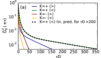
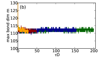
Figure 1: (Color online) Panel (a): Imaginary time correlation functions $\widetilde{G}^{\gtrless}(\tau)$ defined in Eq. (4a) for an impurity model arising in the context of the two-site dynamical cluster approximation to the single-band Hubbard model on the square lattice with next-nearest neighbor hopping $t^{\prime}/t=0.3$, half-band width $D=4t$, interaction $U=2.5D$ and band filling $n=0.96$ in the paramagnetic phase. See Ref. Ferrero et al., 2009 for definition of the model and the meaning of the orbital (patch) quantum number “$K=\pm$”. The dashed line is obtained using linear prediction for times $\tau D\geq 200$. Panel (b): Maximal bond dimension $m$ of time evolved states. The MPS computation used a Hamiltonian representation of the impurity model with $L_{c}=2$ correlated sites and $L_{b}=14$ bath sites. The hybridization function of the impurity model $\Lambda^{\text{discr}}$ was fitted using Eq. (12) for $\beta_{\text{eff}}=315/D$ and $\alpha=0$. For the ground state optimization, we enforced a maximal bond dimension of $m=300$. The Krylov time evolution used a time step of $\Delta t=0.1/D$ and allowed for a maximal global truncation error of $10^{-4}$ at each time step adjusting bond dimensions automatically. This leads to an immediate decay of $m$ at $\tau\simeq 0$ from $m=300$ down to $m\simeq 110$, as seen in panel (b). We used the global SU(2) symmetry of the Hamiltonian to reach these low values of the bond dimension.

While it is not essential in principle, we evaluate Eq. (4) using a Krylov algorithm (Hochbruck and Lubich, 1997), which represents the time evolution operator in a local Krylov space and is able to treat Hamiltonians with long-ranged interactions. Before performing a time evolution computation, one has to compute the initial state $|\psi_{0}^{\gtrless}\rangle$ using an MPS optimization of the ground state. As impurity models come with open boundary conditions, this is well suited for DMRG. We discuss this optimization for typical DMFT Hamiltonians in Appendix A.1.

Figure 1 presents representative results based on parameters obtained from a two-site DMFT solution of the Hubbard model. Figure 1(a) shows the time evolution of $\widetilde{G}^{\gtrless}(\tau)$ out to times as long as 350 times the basic timescale (inverse half-bandwidth $D$) of the model, which suffices to converge $\widetilde{G}^{\gtrless}(\tau)$ to a precision of $5\cdot 10^{-4}$. Figure 1(b) demonstrates the key advantage that makes this computation possible: the lack of growth of maximal bond dimensions $m$ with time of the associated imaginary-time evolved states $|\psi^{\gtrless}(\tau)\rangle=e^{-(H-E_{0})\tau}|\psi_{0}^{\gtrless}\rangle$. The imaginary time-evolution operator does not create entanglement as it projects on the lowly entangled ground state.

Figure 1(a) reveals additional information about the nature and rate of convergence of $\widetilde{G}^{\gtrless}(\tau)$. In the insulating phase, $H$ has a gap and $\widetilde{G}^{\gtrless}(\tau)$ decays exponentially irrespective of whether one considers a finite system or the thermodynamic limit. In the metallic phase, $\widetilde{G}^{\gtrless}(\tau)$ decays algebraically in the thermodynamic limit. For a finite system though, there always remains a small gap, and even though the decay resembles an algebraic decay for short times, it always becomes exponential at long times. The exponential decay can be exploited to speed up computations considerably by a simple technique known as linear prediction (Press et al., 2007; White and Affleck, 2008; Barthel et al., 2009; Wolf et al., 2015). This technique is an efficient formulation of the fitting problem for the ansatz function $f(\tau)=\sum_{n}\alpha_{n}e^{\beta_{n}\tau}$, $\alpha_{n},\beta_{n}\in\mathbb{C},\tau\in\mathbb{R}$, which can then be used to reliably extrapolate functions with an exponentially decaying envelope. This is illustrated by the dashed black line in Fig. 1(a), which has been fitted to match $\widetilde{G}^{\gtrless}(\tau)$ for $\tau D\in[150,200]$ and was then extrapolated for higher times. The solid green line, by contrast, is the result of the MPS computation. Agreement can be seen to be perfect.

II.3 Physical Green’s functions

Of particular interest in the rest of this paper are the imaginary time Green’s functions $G^{\text{mat}}(\tau)$ defined via

$$G^{\text{mat}}(\tau)=-\theta(\tau)\widetilde{G}^{>}(\tau)+\theta(-\tau)\widetilde{G}^{<}(\tau),$$ (5)

whose Fourier transform gives the Matsubara Green’s function

$$G^{\text{mat}}(i\omega_{n})=\int_{-\infty}^{\infty}d\tau\,e^{i\omega_{n}\tau}G^{\text{mat}}(\tau),$$ (6)

at zero temperature, where $\omega_{n}=(2n+1)\pi/\beta$ and $\beta\rightarrow\infty$. We shall also be interested in the retarded real-time Green’s function

$$G^{\text{ret}}(t)=-i\theta(t)(\widetilde{G}^{>}(it)+\widetilde{G}^{<}(it)),$$ (7)

from which the retarded frequency-dependent Green’s function is obtained as

$$G^{\text{ret}}(\omega)=\int_{-\infty}^{\infty}dt\,e^{i(\omega+i0^{+})t}G^{\text{ret}}(t).$$ (8)

In numerical practice, we evaluate the Fourier transforms leading to (6) and (8) approximately as

$$G^{\text{mat}}(i\omega_{n}) =-\int_{0}^{\tau_{\text{max}}}\!\!\!d\tau\,\widetilde{G}^{>}(\tau)e^{i\omega_{n}t}+\int_{-\tau_{\text{max}}}^{0}\!\!\!\!\!\!d\tau\,\widetilde{G}^{<}(\tau)e^{i\omega_{n}t},$$

$$G^{\text{ret}}(\omega) =-i\int_{0}^{t_{\text{max}}}\!\!\!dt\,\big{[}\widetilde{G}^{>}(it)+\widetilde{G}^{<}(it)\big{]}e^{i\omega t},$$ (9)

with cutoff times $\tau_{\text{max}}$ and $t_{\text{max}}$. This approximation is only controlled if we are able to reach long enough times $\tau_{\text{max}}$ and $t_{\text{max}}$, such that $\widetilde{G}^{\gtrless}(\tau)$ and $\widetilde{G}^{\gtrless}(it)$ have converged to zero to any desired accuracy.

In contrast to a computation on the imaginary axis, reaching arbitrarily long times $t_{\text{max}}$ on the real axis is prohibited by a logarithmic growth of entanglement, which comes with a power-law growth of bond dimensions. In addition, finite-size effects are a severe source of errors because the long-time behavior is determined by the bath size. For a numerically exact computation, one has to choose the system large enough to observe exponential “pseudo-convergence” of $\widetilde{G}^{\gtrless}(it)$ to zero before finite-size effects are resolved (Wolf et al., 2015). In the context of the present paper, we deal with small system sizes and will never observe pseudo-convergence. In particular there is no exponential pseudo-convergence, so that linear prediction cannot be employed (Wolf et al., 2015). Therefore, when computing the real-frequency spectral function after converging the DMFT loop, one has to use the further approximation of damping the finite-size effects that emerge at long times by computing, instead of $G^{\text{ret}}(\omega)$ in (9),

$$G^{\text{ret}}_{\eta}(\omega) =-i\int_{0}^{\infty}\!\!\!dt\,\big{[}\widetilde{G}^{>}(it)+\widetilde{G}^{<}(it)\big{]}e^{i\omega t}e^{-\frac{\eta^{2}t^{2}}{2}},$$ (10)

which yields the broadened spectral function $A_{\eta}(\omega)=-\frac{1}{\pi}\text{Im}G^{\text{ret}}_{\eta}(\omega)=\frac{1}{\sqrt{2\pi}\eta}\int d\omega^{\prime}A(\omega^{\prime})e^{-\frac{(\omega-\omega^{\prime})^{2}}{2\eta^{2}}}$. Instead of a Gaussian damping and broadening, one could also use an exponential damping leading to Lorentzian broadening, which damps out the original time-evolution information more strongly, though.

Before presenting detailed benchmark results for the solution of DMFT using imaginary-time evolution of MPS, let us clarify which price we have to pay for profiting from the great advantage of not facing entanglement growth. We do this by comparing the imaginary-time approach (itMPS) to approaches that solve the DMFT loop on the real axis.

III Comparison of imaginary-axis with real-axis computations

The self-consistency equation in DMFT relates an impurity model specified by a hybridization function and a self energy to a lattice model specified by a lattice Hamiltonian and the same self energy. We discuss the issues using the example of the dynamical cluster approximation to the single-band Hubbard model

$$G_{K}^{\text{latt}}(z) =\frac{N_{c}}{N}\sum_{k\in\mathcal{P}_{K}}\frac{1}{z+\mu-\varepsilon_{k}-\Sigma_{K}(z)},$$ (11)

$$\stackrel{{\scriptstyle!}}{{=}}\big{[}z+\mu-\varepsilon_{K}-\Sigma_{K}(z)-\Lambda_{K}(z)\big{]}^{-1}=G_{K}^{\text{imp}}(z).$$

Here $\varepsilon_{k}$ denotes the single-particle dispersion of the lattice and $\mu$ is the chemical potential. In the dynamical cluster approximation, the Brillouin zone, consisting in $N$ momentum vectors $k$, is covered by $N_{c}$ (for single-band $L_{c}=N_{c}$) equal-area tiles (patches), labelled here by $P_{K}$ and the self energy is taken to be piecewise constant, with being a potentially different function of frequency in each tile. The impurity model is specified by the on-site energy $\varepsilon_{K}$ and the hybridization function $\Lambda_{K}(z)$, which is to be determined using the fixed point iteration referred to as the DMFT loop. The loop works as follows: make an initial guess for $\Lambda_{K}(z)$; compute $\Sigma_{K}(z)=\omega+\mu-\varepsilon_{K}-\Lambda_{K}(z)-[G_{K}^{\text{imp}}(z)]^{-1}$, then update $\Lambda_{K}$ via $\Lambda_{K}(z)=z+\mu-\varepsilon_{K}-\Sigma_{K}(z)-[G_{K}^{\text{latt}}(z)]^{-1}$ and repeat this procedure until convergence.

We discuss two aspects of the comparison of real- and imaginary-frequency solutions of the DMFT self-consistency equation (11). The first has to do with the number of bath sites needed to obtain a solution of the self-consistency equation. The second is the accuracy to which the spectral functions of physical interest can be reproduced.

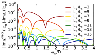
Figure 2: (Color online) Fit of the hybridization function in the two-site DCA problem studied in Figs. 1 and 3, but here for the case $U=0$. The minimization (12) was done using $\alpha=0$ and a frequency grid defined by $\beta_{\text{eff}}=100/D$ and a cutoff frequency of $\omega_{c}=6D$. Evidently, the quality of the fit does not improve any more for $L_{b}/L_{c}\gtrsim 9$.

The DMFT self-consistency equation (11), defines the hybridization function $\Lambda_{K}$ as a continuous function in terms of the difference between the computed self energy and the inverse of the lattice Green’s function. In DMRG-type methods, the hybridization function $\Lambda_{K}$ is approximated as the hybridization function $\Lambda^{\text{discr}}_{K}$ of a discrete impurity model, which is the sum of a number of poles. If the number of poles is too small one cannot construct a meaningful approximation on the real axis (de Vega et al., 2015) and a DMFT loop cannot be converged. For this reason DMRG-based solutions of DMFT up to now (García et al., 2004; Nishimoto et al., 2004; Karski et al., 2005; Nishimoto et al., 2006; García et al., 2007; Karski et al., 2008; Peters, 2011; Ganahl et al., 2014a, b; Wolf et al., 2014a, b), all of which were real axis computations, have been performed using numbers of bath sites of at least $L_{b}/L_{c}\gtrsim 30$, and in the case of the single-band Hubbard model, even much more $L_{b}/L_{c}\gtrsim 120$. Use of such a large number of bath sites means that with modest broadening the hybridization function can be reasonably approximated as a continuum, enabling a stable solution of Eq. (11).

By contrast, formulating the problem on the imaginary axis (as is typically done in standard ED solvers where the number of bath sites is strictly limited) automatically smoothens the hybridization function $\Lambda^{\text{discr}}_{K}$ and permits a stable solution. From the imaginary axis solution one must then determine the discrete set of bath parameters to represent $\Lambda^{\text{discr}}_{K}$. This is typically done (Caffarel and Krauth, 1994; Liebsch and Ishida, 2012; Go and Millis, 2015) by numerical minimization of a cost function defined as

$$\chi^{2}=\frac{1}{N_{\text{fit}}}\sum_{n=1}^{N_{\text{fit}}}\omega_{n}^{-\alpha}|\Lambda_{K}(i\omega_{n})-\Lambda_{K}^{\text{discr}}(i\omega_{n})|^{2}.$$ (12)

Here, $\alpha$ defines a weighting function $\omega_{n}^{-\alpha}$. Choosing $\alpha>0$, e.g. $\alpha=1$, attributes more weight to smaller frequencies (Senechal, 2010; Liebsch and Ishida, 2012; Go and Millis, 2015), which we find helpful when using small bath sizes $L_{b}/L_{c}<5$. To define the frequency grid for the fit $\omega_{n}=(2n+1)\pi/\beta_{\text{eff}}$, one defines a fictitious inverse temperature $\beta_{\text{eff}}$, which has no physical significance. We further employ a cutoff frequency $\omega_{c}$, which implies a finite number $N_{\text{fit}}$ of fitted Matsubara frequencies.

If one tries to define an analogous cost function for the real axis, the result is useless as then $\Lambda_{K}^{\text{discr}}(\omega+i0^{+})$ is a sum of poles, whereas the hybridization function $\Lambda_{K}(\omega+i0^{+})$, as encountered in (11), is continuous (de Vega et al., 2015). One can overcome this problem only when using a Lindbladt formalism (Dorda et al., 2014), which increases the complexity of the problem substantially.

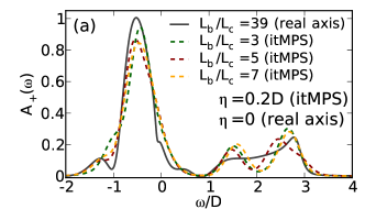
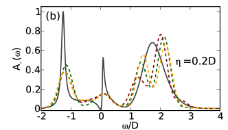
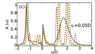
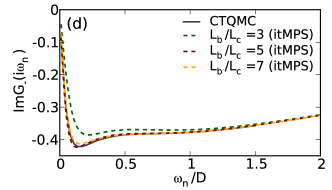
Figure 3: (Color online) Real- and imaginary-frequency Green’s functions computed by converging the DMFT self-consistency equation Eq. (11) for the two-site dynamical cluster approximation to the single-band Hubbard model on the square lattice with next-nearest neighbor hopping $t^{\prime}/t=0.3$, half-band width $D=4t$, interaction $U=2.5D$, and band filling $n=0.96$ in the paramagnetic phase (as in Fig. 1). See Ref. Ferrero et al., 2009 for definition of the model and the meaning of the orbital (patch) quantum number “$K=\pm$”. Panels (a-c): Electron spectral function $A(\omega)=-\frac{1}{\pi}\text{Im}G^{\text{ret}}(\omega)$ obtained by converging on imaginary-frequency axis (itMPS) using number of bath sites and broadenings as specified in the figure, and compared to unbroadened ($\eta=0$) real-frequency axis computation using $L_{b}/L_{c}=39$ bath sites per correlated site of Ref. Wolf et al., 2014a. Panel (d): Converged Matsubara Green’s function for number of bath sites shown, compared to numerically exact quantum Monte-Carlo result of Ref. Ferrero et al., 2009, computed at $\beta=200/D$.

The minimization of (12) is done using using standard numerical optimization. The optimization in the initial DMFT iteration should be done using a global optimization scheme (Wales and Doye, 1997), and in subsequent iterations using a local optimization scheme (e.g. conjugate gradient), which takes as an initial guess for the new bath parameters the values of the previous iteration. Figure 2 shows the convergence of the fit of the hybridization function with the number of bath sites $L_{b}/L_{c}$. For $L_{b}/L_{c}=7$ one already obtains errors as little as $\simeq 10^{-3}$ and for values $L_{b}/L_{c}\gtrsim 9$ the quality of the fit already stops improving. It is at this point, where we (and all ED-like techniques) face the problem of “analytic continuation” encountered in CTQMC, namely that Green’s functions on the imaginary axis encode information in a much less usable form than on the real axis.

Consider again the example of the two-site DCA for the single-band Hubbard model on the square lattice. In Ref. Wolf et al., 2014a, this problem has been solved entirely on the real axis using $L_{b}/L_{c}=39$ bath orbitals. Here, we converge the DMFT loop on the imaginary axis and compute the spectral function in a final real-time evolution using $L_{b}/L_{c}=3,5,7$ bath orbitals. We compare both solutions in Fig. 3. Whereas for the (central) momentum patch “$+$” shown in Fig. 3(a), we find satisfactory agreement of the imaginary-axis with the real-axis calculation, this is not the case for the (outer) momentum patch “$-$” shown in Fig. 3(b), even though the corresponding imaginary-axis Green’s function is well reproduced, see Fig. 3(d). Evidently, in Fig. 3(b), the central peak and the pseudo-gap at the Fermi edge are smeared out by a broadening $\eta=0.2D$ that hides finite-size effects to a large degree. Reducing the broadening to $\eta=0.05D$ as shown in Fig. 3(c), again reveals the pseudo-gap and the central peak; but together with unphysical finite-size effects. We observe that the nature of these finite-size effects is qualitatively comparable when using different numbers of bath sites $L_{b}/L_{c}=3,5,7$. Already for $L_{b}/L_{c}=3$, we obtain reasonable results. On the imaginary axis, by contrast, $L_{b}/L_{c}=5,7$ still improve over $L_{b}/L_{c}=3$ and almost agree with the numerically exact QMC data for $\beta=200/D$ of Ref. Ferrero et al., 2009, see Fig. 3(d). However we emphasize that even with the modest number of bath sites used here the basic features of the spectral function are reproduced (for example the areas in given frequency ranges).

IV Three-band calculations

IV.1 Three-band model in single-site DMFT

We now demonstrate the power of the method by applying it to three-band problems in the single-site approximation (where comparison to existing calculations can be made) and the two-site approximation. Both was hitherto not accessible to DMFT+DMRG computations.

We study the three-band Hubbard-Kanamori model with Hamiltonian (omitting the site index $i$ in the following definition of $H_{\text{loc},i}$)

$$H =\sum_{k,a,b,\sigma}\varepsilon^{ab}_{k}d^{\dagger}_{k,a,\sigma}d_{k,b,\sigma}+\sum_{i}H_{\text{loc},i}$$

$$H_{\text{loc}} =-\sum_{a,\sigma}(\mu-\Delta_{a})n_{a,\sigma}$$

$$\quad+\sum_{a}Un_{a,\uparrow}n_{a,\downarrow}$$ (13)

$$\quad+\sum_{a>b,\sigma}\Big{[}U^{\prime}n_{a,\sigma}n_{b,-\sigma}+(U^{\prime}-J)n_{a,\sigma}n_{b,\sigma}\Big{]}$$

$$\quad-\sum_{a\neq b}J(d^{\dagger}_{a,\downarrow}d^{\dagger}_{b,\uparrow}d_{b,\downarrow}d_{a,\uparrow}+d^{\dagger}_{b,\uparrow}d^{\dagger}_{b,\downarrow}d_{a,\uparrow}d_{a,\downarrow}+\text{h.c.}),$$

where $i$ labels sites in a lattice and $k$ wave vectors in the first Brillouin zone, $n_{i,a,\sigma}=d^{\dagger}_{i,a,\sigma}d_{i,a,\sigma}$ is the density of electrons of spin $\sigma$ in orbital $a$ on site $i$, $\mu$ is the chemical potential, $\Delta_{a}$ is a level shift for orbital $a$, $\varepsilon^{ab}_{k}$ is the band dispersion, $U$ is the intra-orbital and $U^{\prime}$ the inter-orbital Coulomb interaction, and $J$ is the coefficient of the Hund coupling and pair-hopping terms. We adopt the conventional choice of parameters, $U^{\prime}=U-2J$, which follows from symmetry considerations for $d$-orbitals in free space and holds (at least for reasonably symmetric situations) for the $t_{2g}$ manifold in solids (Georges et al., 2012).

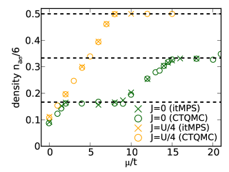
Figure 4: (Color online) Density per orbital as function of chemical potential for three-band Hubbard-Kanamori model Eq. (13) using the semi-elliptic density of states Eq. (14) and $U=12t$, obtained from single-site DMFT approximation evaluated using imaginary MPS (crosses) and CTQMC data (circles, Figure 1 of Ref. Werner et al., 2009, inverse temperature $\beta=50/t$). In the DMRG computations the bath fitting was performed using $\beta_{\text{eff}}=100/t$, $\omega_{c}=6t$ and $\alpha=1$ with three bath sites per correlated site ($L_{b}/L_{c}=3$). The maximal matrix dimensions was $m=300$ for the ground state calculation, exploiting the SU(2) symmetry, which leads to the high precision $\langle(H-E)^{2}\rangle\simeq 10^{-14}$. For the time evolution, we computed $\widetilde{G}_{a}^{\gtrless}(\tau)$ in (4a) in steps of $\Delta\tau=0.1/t$ allowing a global truncation error of $5\cdot 10^{-4}$ per step, up to imaginary time $\tau_{\text{max}}=100/t$ and used linear prediction for higher times.

We study the orbital-diagonal and orbital-degenerate case ($\Delta_{a}=0$) on the Bethe lattice, i.e. the non-interacting density of states is semi-elliptic,

$$A_{a,0}(\omega)=\frac{1}{\pi t}\sqrt{1-(\tfrac{\omega}{2t})^{2}}.$$ (14)

In the single-site approximation, the impurity Hamiltonian used within DMFT is given by

$$H =H_{\text{loc}}+H_{\text{coupl}}+H_{\text{bath}},$$

$$H_{\text{coupl}} =\sum_{l,a,\sigma}V_{l,a,\sigma}~{}d^{\dagger}_{a,\sigma}c_{l,a,\sigma}+\text{h.c.},$$ (15)

$$H_{\text{bath}} =\sum_{l,a,\sigma}\varepsilon_{l,a.\sigma}~{}c^{\dagger}_{l,a,\sigma}c_{l,a,\sigma},$$

where $c^{\dagger}_{l,a,\sigma}$ creates a fermion in the bath orbital $l$, $V_{l,a,\sigma}$ describes the coupling of the impurity to the orbital $l$, and $\varepsilon_{l,a.\sigma}$ denotes the potential energy of orbital $l$. The hybridization function is then given by

$$\Lambda_{a,\sigma}^{\text{discr}}(z)=\sum_{l=1}^{L_{b}/L_{c}}\frac{|V_{l,a,\sigma}|^{2}}{z-\varepsilon_{l,a.\sigma}}.$$ (16)

Figure 4 compares the dependence of the particle density $n$ on the chemical potential $\mu$ obtained by the MPS methods used here to those obtained by numerically exact CT-QMC methods (Werner et al., 2009). The plateaus in $n(\mu)$ are the Mott insulating regimes of the phase diagram. The agreement is very good in general, confirming the reliability of our new procedure even with only three bath sites per correlated site. This leads to an extremely cheap computation, for which a single iteration of the DMFT loop took about $30\text{\,}\mathrm{m}\mathrm{i}\mathrm{n}$ on two $2.8\text{\,}\mathrm{G}\mathrm{H}\mathrm{z}$ cores (see Appendix A.2 for more details).

In panel (a) of Fig. 5 we show a more stringent test, namely the dependence of the self energy on Matsubara frequency, in a parameter regime where the self energy was previously found Werner et al. (2008) to exhibit an anomalous $\omega^{\frac{1}{2}}$ frequency dependence and (in some regimes) a non-zero intercept as $\omega\rightarrow 0$. These phenomena are associated with a spin-freezing transition Werner et al. (2008, 2009).

Panel (a) of Figure 5 shows that the known low frequency $\omega\lesssim t$ self energy is already accurately reproduced even for the computationally inexpensive choice of $L_{b}/L_{c}=3$, although one observes deviations for the high-frequency behavior. The deviations at high frequency decrease as the number of bath sites is increased, although full convergence at all frequencies has not been demonstrated. Panel (b) of Fig. 5 shows that the deviations are linked to the impossibility of fitting the hybridization function equally well for all frequencies using only a small number of bath sites. The large deviations at high frequencies are due to the choice $\alpha=1$ in (12), which enforces good agreement for low frequencies and allowed to successfully reproduce the MIT transition in Fig. 4. Increasing the number of bath sites to $L_{b}/L_{c}=5$ leads to a much better approximation of the hybridization function also for high frequencies, with concomitant improvement in the self-energy (Fig. 5(a)).

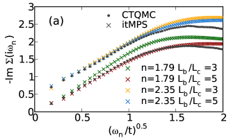
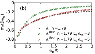
Figure 5: (Color online) Imaginary part of Matsubara axis self energy $\Sigma$ (panel (a)) and imaginary part of hybridization function $\Lambda$ (panel (b)) for densities shown obtained from converged itMPS solution of single-site DMFT for three-band Hubbard-Kanamori model (IV.1) for $U=8t$ and $J=U/6$. Crosses (color online) represent itMPS data and black circles depict CTQMC data from Figure 3 of Ref. Werner et al., 2008, computed at inverse temperature $\beta=100/t$. We choose all parameters as described in the caption of Fig. 4, in particular, for the bath fitting (12), we use $\beta_{\text{eff}}=100/t$, $\omega_{c}=6t$ and $\alpha=1$. Choosing $\alpha=1$ enforces agreement for low frequencies at the price of disagreement at high frequencies, which is observed in both panels (a) and (b). In panel (b), $\Lambda$ denotes the hybridization function that is fitted with the hybridization function $\Lambda^{\text{discr}}$ of the discrete impurity model.

IV.2 Three-band model in two-site DCA

We now present results obtained using a two-site DCA approximation to the three-band model of the previous section. For this problem there are no low-temperature results available in the literature. The size of the problem is beyond the scope of standard ED. The truncated configuration interaction (CI) impurity solver (Knizia and Chan, 2012) allows to access a relatively high number of bath sites but is limited in the number of correlated sites: e.g. in Ref. Lin and Demkov, 2013b, a problem with $L_{c}=3$ and $L_{b}=30$ was computed, and in Ref. Go and Millis, 2015, one with $L_{c}=4$ and $L_{b}=20$. The three-band two-site DCA though has $L_{c}=6$ correlated sites and it remains to be seen whether this is in reach for the CI solver. The problem is also challenging for standard CTQMC. Recent technical improvements on mitigating the sign problem (Nomura et al., 2014) enabled Ref. Nomura et al., 2015 to treat this model at the temperature of $T=0.025D$ with $D$ the half bandwidth, which required large computational resources. This temperature is relatively high as the authors stated that in the study of a simpler two-band two-site model, where they reached $T=0.0125D$, it was “intractable” to reach low enough temperatures to clarify whether bad metal/spin freezing behavior was intrinsic or not (Nomura et al., 2014).

We study the model on the two-dimensional square lattice, i.e. using $\varepsilon_{k}^{ab}=-2t\left(\cos k_{x}+\cos k_{y}\right)\delta^{ab}$. We use the momentum patching of Ref. Ferrero et al., 2009; this definition is also used in the single-band computations of Figs. 1 and 3. We note that this model is not directly relevant to layered materials where the $t_{2g}$ orbitals are relevant, because in the physical situation the two dimensionality will break the three-fold orbital degeneracy. However the system is well defined as a theoretical model and useful to demonstrate the power of our methods.

As is the case for the CI method, the DMRG method used here is easily able to treat a large number of bath sites if the number of correlated sites is small: for $L_{c}=1$, DMRG has already often be proven to treat $L_{b}>120$ bath sites, and for $L_{c}=2$, $L_{b}>80$ is easily accessible (Wolf et al., 2014a, b). However for more correlated sites, the number of bath sites that can be added at given computational cost decreases. For $L_{c}=6$, we use $L_{b}=18$, i.e. $L_{b}/L_{c}=3$, which we have shown to be sufficient to produce reliable results in the single-site case without requiring overly large computational resources (computation time of several hours per DMFT iteration on two cores).

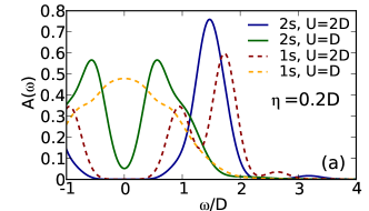
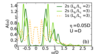
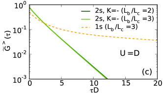
Figure 6: (Color online) Comparison of results obtained using MPS methods with for $L_{b}/L_{c}=3$ for single site (1s) and two-site (2s) DMFT approximations to the Hubbard-Kanamori model (13) on the two-dimensional square lattice with half bandwidth $D=4t$, $\varepsilon_{k}^{ab}=-2t\left(\cos k_{x}+\cos k_{y}\right)\delta^{ab}$, $U^{\prime}=U-2J$, $J=U/4$ and $n=3$ ($\mu=5U/2-5J$), that is, in the particle-hole symmetric case. Panel (a): spectral functions for broadening $\eta=0.2D$; panel (b) broadening $\eta=0.05D$. In panel (c), we show the imaginary-time evolution of $\widetilde{G}^{>}(\tau)$ as defined in (4a), confirming by comparison to a calculation for a smaller bath $L_{b}/L_{c}=2$ that this quantity has been converged with respect to the bath size. The maximal bond dimension for the ground state search was $m=1000$.

We have tested the two-site calculation by converging the DMFT loop for the three-band Hubbard model Eq. (IV.1) with $U^{\prime}$ and $J=0$ and comparing the results with a corresponding two-site single-band DCA. Perfect agreement is obtained (not shown). Non-zero values of $U^{\prime}$ and $J$ create additional entanglement and make computations more costly. It is then a decisive question whether a real-space or a momentum-space representation of the impurity-cluster is less entangled. We discuss this in Appendix B finding that for the single-band Hubbard interaction, both representations yield similar entanglement, whereas for the Hubbard-Kanamori interaction, the real-space representation is much less entangled. Computational cost is therefore tremendously reduced by using the real-space representation, which comes with an off-diagonal hybridization function. This is the opposite behavior as observed for QMC, where the off-diagonal hybridization function creates a severe sign problem. We further note that in the real-space representation, strong interactions yield a less and less entangled impurity problem, as electrons become more and more localized.

We now present results for the more physically relevant case $U^{\prime}=U-2J$ with $J=U/4$. For these parameters, at half filling the critical interaction for the MIT in the single-site DMFT approximation is $U_{c}\simeq 1.3D$ (de’ Medici et al., 2011). Fig. 6(a) shows that our results are consistent with this estimate: the dashed lines depict the single-site (1s) results, showing a metallic solution (spectral function non-zero at $\omega=0$) for $U=D$, and an insulating solution (spectral function zero at $\omega=0$) for $U=2D$. In the two-site (2s) DCA (solid lines), by contrast, the critical value $U_{c}$ for the MIT is lowered. Even at $U=D$ the $\omega=0$ spectral function is zero (the small non-zero value in panel (a) is an effect of broadening, as seen in panel (b)). The different nature of the metallic and insulating solutions is also visible on the imaginary axis in the different nature of the decay of the imaginary-time Green’s function. This is plotted in Fig. 6(c) for $U=D$; clearly, a power-law decay is observed for the metallic solution obtained in the single-site DMFT, whereas an exponential decay is obtained for the insulating solution obtained within the two-site DCA.

V Conclusion

This paper introduces an imaginary-time MPS (itMPS) solver for DMFT and shows that it can treat complex models, not easily accessible with other methods, at modest computational cost. This development establishes DMRG as a flexible low-coast impurity solver for realistic problems, such as encountered in the study of strongly-correlated materials. The crucial advance stems from the fact that imaginary-time evolution does not create entanglement, and hence allows to compute Green’s functions numerically exactly, provided a ground state calculation is feasible.

The method can be improved in many ways. In particular, different representations of the impurity problem exhibit different degrees of entanglement, so optimizing the representation of the impurity problem is a promising route. Ideas from ED approaches for constructing relevant subspaces (Lu et al., 2014; Zgid et al., 2012; Lin and Demkov, 2013a, b) of the Hilbert space may lead to further improvements. Such techniques have been successfully combined with MPS (Ma and Ma, 2013). Another route to reduce computational effort and by that reach even more complex models could consist in performing computations for the reduced dynamics of the impurity (Cohen et al., 2013), or making use of extremely cheap algorithms for computing the Green’s function at elevated temperatures (Savostyanov et al., 2014). Finally, we note that using MPS as an impurity solver makes accessing entanglement as a quantity for understanding the properties of the embedded impurity cluster very easily accessible. Proposals in this direction have been made for cellular DMFT (Udagawa and Motome, 2015) and for impurity models generally (Lee et al., 2015).

VI Acknowledgements

FAW thanks G. K.-L. Chan for stressing the relevance of converging the DMFT loop on the imaginary-frequency axis, and N.-O. Linden for helpful discussions. AJM and US acknowledge the hospitality of the Aspen Center for Physics NSF Grant 1066293 during the inception of this work. FAW and US acknowledge funding by FOR1807 of the DFG. AJM and AG were supported by the US Department of Energy under grant ER-046169.

Appendix A Further technical details

A.1 Ground state optimization

The main challenge in solving the ground state problem of a typical cluster-bath Hamiltonian as encountered in DMFT, stems from the fact that DMRG is a variational procedure that is initialized with a random state, which is then optimized locally. A local optimization procedure is slow when optimizing a global energy landscape. In addition, the local optimization is prone to getting stuck in local minima, if no “perturbation steps that mix symmetry sectors” are applied. The standard perturbation techniques for single-site DMRG (White, 2005; Dolgov and Savostyanov, 2014; Hubig et al., 2015) rely on “perturbation terms” that are produced by contracting the Hamiltonian with the MPS. If the Hamiltonian itself does not contain terms that mix the symmetry sector, these methods do not work.

A typical cluster-bath Hamiltonian has both features, a global variation of the potential energy and parts that are not connected with symmetry mixing terms, such as in the three-band Hubbard Kanamori model at $J=0$. This situation is sketched in Fig. 7.

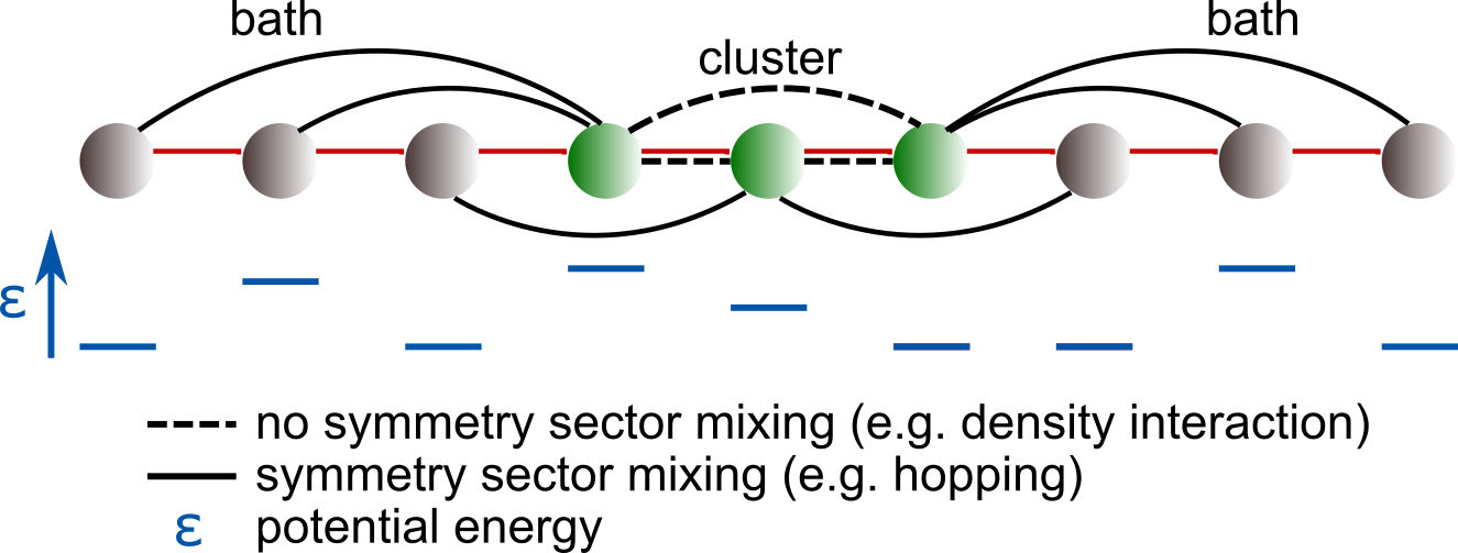
Figure 7: (Color online) Sketch of a typical cluster-bath Hamiltonian ($L_{c}=3$, $L_{b}=6$) when it’s mapped to a one-dimensional chain. Dashed lines depict couplings that do not mix symmetry sectors, and solid lines depict couplings that mix symmetry sectors.

In Ref. Wolf et al., 2014a, the models under study allowed to solve this problem using the non-interacting solution. For the general models studied in the present paper, an unbiased numerical technique has to be employed. What we do in practice, is to first find the ground state of a system with additional symmetry-mixing couplings (denoted as red solid lines in Fig. 7) that are then adiabatically switched off. In practice, we sweep 5 to 10 times with additional hoppings of 10% magnitude of the physical hoppings, and another 5 to 10 times with additional hoppings of 1% magnitude. After these preliminary sweeps, the quantum number (e.g. particle number) distribution has globally converged, and we can continue with converging the ground state of the exact Hamiltonian.

A.2 Convergence of DMFT iteration

The calculations for the three-band single-site DMFT in Sec. IV.1 are only trivially parallelized using one core to compute the imaginary time evolution of each the particle ($>$) and the hole ($<$) Green’s functions $\widetilde{G}_{a}^{\gtrless}(\tau)$.

In Fig. 8, we show the convergence DMFT loop for the single-site DMFT for the three-band Hubbard-Kanamori model as studied in Fig. 5. Fig. 8(a) shows the convergence of the Matsubara Green’s function down to a precision of $10^{-3}$. Figs. 8(b) and (c) show the convergence of the density and of the ground state energy per particle, respectively. Fig. 8(d) shows the computation time. An iteration on the Matsubara axis takes about $30\text{\,}\mathrm{m}\mathrm{i}\mathrm{n}$. The final real-axis computation (iteration 31) is considerably more expensive, but can still be optimized.

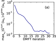
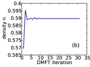
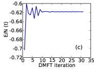
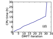
Figure 8: (Color online) Single-site DMFT for three-band Hubbard-Kanamori model as studied in Fig. 5. Here for the case $n=1.77$ ($\mu=5.0$) and $L_{b}/L_{c}=3$. To obtain the solution for $n=1.79$ as shown in Fig. 5, we chose $\mu=5.1$ and started from the $n=1.77$ solution. Panel (a): Convergence of Matsubara Green’s function in the DMFT loop, starting from the non-interacting solution. Panel (b): Convergence of the density in the DMFT loop. Panel (c): Convergence of the ground state energy per particle in the DMFT loop. Panel (d): Computation time. An iteration on the Matsubara axis takes about $30\text{\,}\mathrm{m}\mathrm{i}\mathrm{n}$. The final real-axis computation (iteration 31) is considerably more expensive, but can still be optimized.

Appendix B Least-entangled representation and off-diagonal hybridization functions

B.1 Geometry and general considerations

In Ref. Wolf et al., 2014b, some of us showed that the star geometry of the impurity problem can have substantially lower entanglement than its chain geometry. In the star geometry, DMRG profits from the small entanglement of the almost occupied states with low potential energy with the almost unoccupied states with high potential energy. A high weight for the superposition of a low- with a high-energy state is physically irrelevant. In the star geometry, DMRG is able to eliminate these superpositions as potential energy is separated locally, i.e. in the same basis in which DMRG optimizes the reduced density matrix in order to discard irrelevant contributions. In principle, as mentioned in Appendix C, ideas from basis selective approaches in exact diagonalization are a different method to account for the fact that many states in the Hilbert space have a negligible weight for the computation of the Green’s function and only few physically relevant states occupy a small fraction of the Hilbert space. Among these are the truncated configuration interaction (CI) (Knizia and Chan, 2012; Lin and Demkov, 2013a, b; Go and Millis, 2015), the basis-selective ED (Lu et al., 2014) or the coupled cluster methods in quantum chemistry. As these methods can be combined with DMRG (Ma and Ma, 2013), they might be a further route to construct efficient representations of the impurity-cluster problem

In the present paper, the question of the least entangled representation of the impurity problem shall be restricted to the question of which basis to choose in a DCA calculation. This is of high relevance also in another context: In the real-space representation, the hybridization function becomes off-diagonal. For CTQMC, this generates a sign problem. In our approach, this doesn’t affect computational cost much in the single-band Hubbard model. It even leads to a tremendous reduction of computational cost for the three-band Hubbard Kanamori interaction.

B.2 DCA in momentum or real space

The complexity of the interaction determines whether the real- or the momentum-space representation of the cluster-bath Hamiltonian is less entangled. In real space, the interaction has a simple form, but the hybridization function has off-diagonal contributions, which result in additional couplings of cluster and bath sites. In momentum space, the hybridization function is diagonal but the interaction becomes off-diagonal. The additional couplings induced by that depend on the complexity of the interaction.

Let us be more concrete. For the two-site case, the discrete Fourier transform yields the even and odd superposition of the real-space cluster.

$$\widetilde{d}_{1}^{\dagger} =\frac{1}{\sqrt{2}}(d_{1}^{\dagger}+d_{2}^{\dagger})$$ (17)

$$\widetilde{d}_{2}^{\dagger} =\frac{1}{\sqrt{2}}(d_{1}^{\dagger}-d_{2}^{\dagger})$$ (18)

where the index of $\widetilde{d}_{K}^{\dagger}$ labels momentum patches $K$ and the index of $d_{i}^{\dagger}$ labels real space cluster sites $i$. There might be further indices labeling spin or orbital.

In real-space, the hybridization function has the form

$$\Lambda_{ij}(z)=\sum_{l=1}^{L_{b}}\frac{V_{il}^{*}V_{jl}}{z-\varepsilon_{l}},$$ (19)

where the symmetry of the real-space cluster imposes $\Lambda_{ij}(z)=\Lambda_{ji}(z)$. In momentum space, the hybridization function is diagonal

$$\widetilde{\Lambda}_{K}(z)=\sum_{l=l_{K}=1}^{L_{b}^{\prime}}\frac{\widetilde{V}_{Kl}^{*}\widetilde{V}_{Kl}}{z-\widetilde{\varepsilon}_{Kl}}$$ (20)

and symmetry is reflected in the reduced number of bath sites per patch $L_{b}^{\prime}=L_{b}/L_{c}$, where $L_{c}=2$ is the number of momentum patches.

We choose to use the momentum representation for the bath discretization, as was done for the real-axis in Ref. Wolf et al., 2014a. While on the real-frequency axis this is the only viable option, the bath fitting on the imaginary-frequency axis via (12) is possible also for the off-diagonal real-space case. In real space, e.g. , particle hole symmetry can be easily imposed in the fitting procedure, while this is not possible in momentum space.

Given the parameters of the momentum space representation obtained by performing a bath fit via (12), we define the parameters of the equivalent real-space representation as follows: In momentum space, bath parameters are indexed by $l_{K}=1,...,L_{b}^{\prime}$, $L_{b}^{\prime}=L_{b}/L_{c}$ and in real space, bath parameters are indexed by $l=1,...,L_{b}$, then

$$\varepsilon_{l} =\widetilde{\varepsilon}_{1,l_{1}=l}\text{ for }l=1,...,L_{b}^{\prime}$$

$$\varepsilon_{l} =\widetilde{\varepsilon}_{2,l_{2}=l-L_{b}^{\prime}}\text{ for }l=L_{b}^{\prime}+1,...,L_{b}$$

$$V_{1l} =V_{2l}=\tfrac{1}{\sqrt{2}}\widetilde{V}_{1,l_{1}=l}\text{ for }l=1,...,L_{b}^{\prime}$$

$$V_{1l} =-V_{2l}=\tfrac{1}{\sqrt{2}}\widetilde{V}_{2,l_{2}=l-L_{b}^{\prime}}\text{ for }l=L_{b}^{\prime}+1,...,L_{b}.$$ (21)

Whereas the momentum-space Hamiltonian has $L_{b}$ non-zero couplings $V_{Kl_{K}}$, the real space Hamiltonian has $L_{c}\times L_{b}$ couplings $V_{il}$. On the other hand, the interaction part generates $L_{c}\times(L_{c}-1)$ additional non-local couplings in the momentum-space representation as compared to the real-space Hamiltonian.

From this one could naively expect that the real-space representation is less entangled if $L_{c}\times(L_{c}-1)>L_{c}\times L_{b}$. Numerical experiments show that the real-space representation is much more favorable than this estimate. For a single-band Hubbard model, we find about the same entanglement in the real space and the momentum space representation, with slight advantages for momentum space. In the three-band Hubbard Kanamori model, the real-space representation is considerably less entangled and leads to a tremendous reduction of computational cost. In particular, we were not able to obtain the results of Fig. 6 in the momentum space representation when using $L_{b}/L_{c}=3$, only for $L_{b}/L_{c}=2$ but then at much higher computational cost.

Appendix C Green’s functions from matrix product states

Even though the following discussion is not needed to set up the imaginary-time real-time impurity solver, it is of general interest in this context and might stimulate further advancements.

A computation of $A(\omega)=\langle\psi_{0}|\delta(\omega-(H-E_{0}))|\psi_{0}\rangle$ via a computation of all eigen states of $H$ is extremely redundant as only a tiny neighborhood $\mathcal{N}=\{|\psi\rangle\big{|}\langle\psi|H|\psi_{0}\rangle\neq 0\}$ of a the single-particle excitation $|\psi_{0}\rangle$ contributes in the sum (inserting identities $\sum_{n}|E_{n}\rangle\langle E_{n}|$) in $A(\omega)$. In ED, this is exploited by systematically constructing the subspace $\mathcal{N}$ by spanning it using particle-hole excitations (Lu et al., 2014; Knizia and Chan, 2012), which might also be a viable route for further developments within DMRG (Ma and Ma, 2013). In DMRG, one needs to make a statement about the entanglement of the states in the subspace $\mathcal{N}$: one might note that these are in general more strongly entangled than the single-particle excitation $|\psi_{0}\rangle$, but should still be much less entangled than the rest of the Hilbertspace. This is illustrated in the sketch Fig. 9.

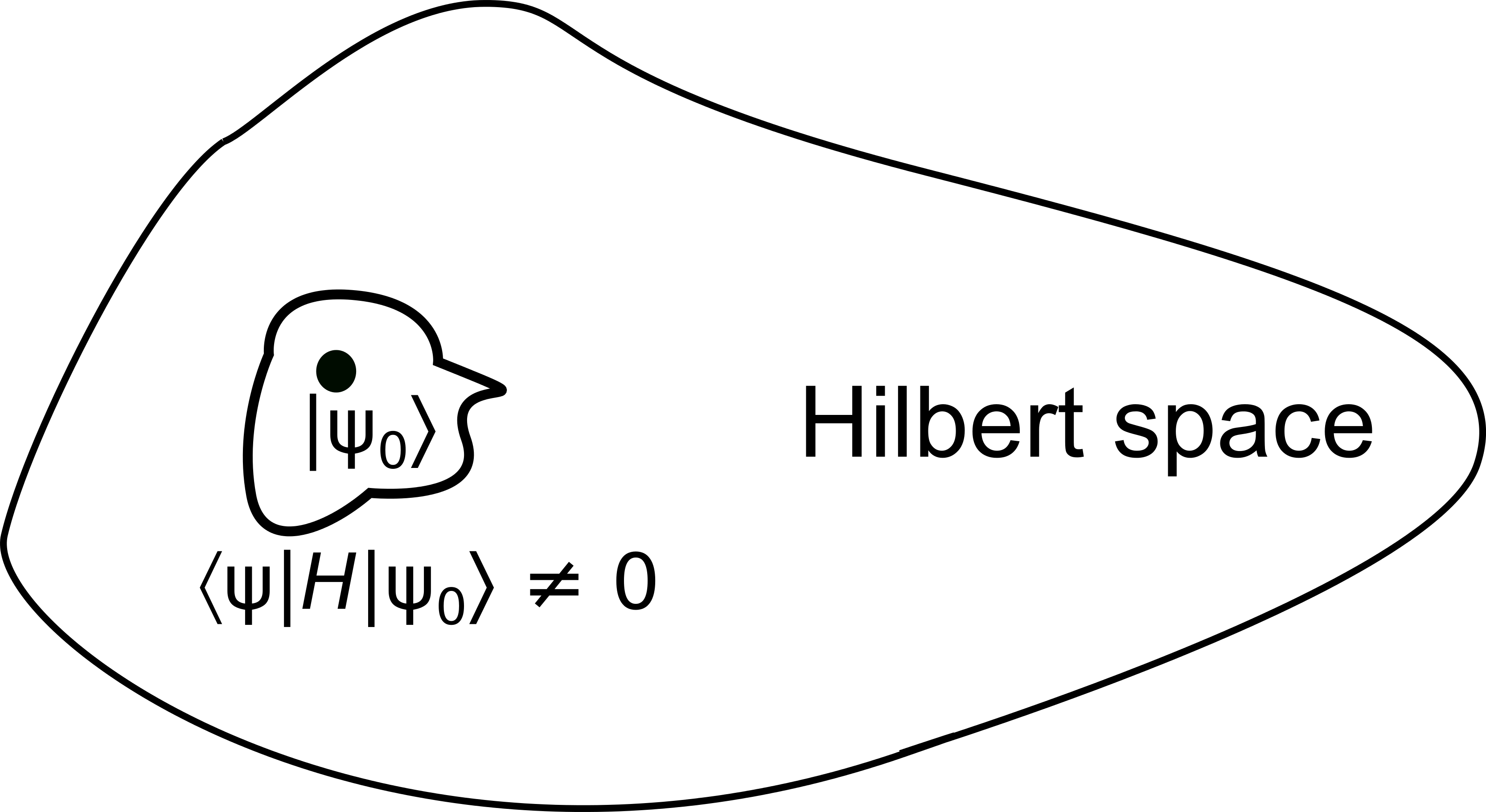
Figure 9: (Color online) Single particle excitation $|\psi_{0}\rangle$ of the ground state $|E_{0}\rangle$ and the subspace $\mathcal{N}=\{|\psi\rangle\,|\,\langle\psi|H|\psi_{0}\rangle\neq 0\}$ of the Hilbert space that is relevant for the computation of a single-particle spectral function of the form $\langle\psi_{0}|\delta(\omega-H)|\psi_{0}\rangle$. The single particle excitation is very lowly entangled, the subspace is more strongly entangled, but still in general more lowly entangled than the rest of the Hilbert space.

In Ref. Wolf et al., 2015, some of us argued that expanding the spectral function in a family of orthogonal functions is a natural way to construct a basis for $\mathcal{N}$, starting from the lowly entangled $|\psi_{0}\rangle$ and successively increasing entanglement of states and thereby computational complexity in a sequence of basis states $|\psi_{n}\rangle$. Ref. Wolf et al., 2015 discussed the expansion of $A(\omega)$ in Chebyshev polynomials $T_{n}(\tfrac{\omega}{a})=\arccos(n\cos(\tfrac{\omega}{a}))$, which are orthogonal with respect to an inner product weighted by $w(x)=\sqrt{1-x^{2}}$ (Weiße et al., 2006), and in the plane waves $\exp(i\omega\tfrac{n}{a})$ (orthogonal with weight function $w(x)=1$), where the energy $a$ is chosen larger than the support of $A(\omega)$. The associated generated sequences of basis states then are

$$|\psi_{n}^{\text{che}}\rangle =2(\tfrac{H-E_{0}}{a}+b)|\psi_{n-1}^{\text{che}}\rangle-|\psi_{n-2}^{\text{che}}\rangle,~{}b\in[-1,1],$$

$$|\psi_{n}^{\text{time}}\rangle =\exp(-i(H-E_{0})\tfrac{n}{a})|\psi_{0}\rangle,$$ (22)

and have different entanglement properties. The states $|\psi_{n}^{\text{time}}\rangle$ associated with time evolution are in general less entangled than the states $|\psi_{n}^{\text{che}}\rangle$ associated with the Chebyshev recursion (Wolf et al., 2015). This is due to the observation that error accumulation in the Chebyshev recursion is worse conditioned than in time propagation (Wolf et al., 2015), which necessitates to keep the error in a single step of the Chebyshev recursion much smaller than in the equivalent time evolution step, which in turn requires to use higher bond dimensions in the Chebyshev recursion making it less efficient. In addition to the statements of Ref. Wolf et al., 2015, we note here that the sequence produced by the Lanczos algorithm,

$$|\psi_{n}^{\text{lan}}\rangle=H-\alpha_{n}|\psi_{n-1}^{\text{lan}}\rangle-|\psi_{n-2}^{\text{lan}}\rangle,~{}\alpha_{n},\beta_{n}\in\mathbb{R}$$ (23)

can be associated with an expansion of the spectral function in polynomials that are orthogonal with respect to an inner product weighted by $w(x)=A(x)$ (Gautschi, 2005). This is very efficient but numerically unstable.

In contrast to the previous methods, which generate an increasingly complex basis when determining the spectral function to a higher and higher precision, correction-vector DMRG aims to optimize a state in frequency space, which a priori contains contributions that have undergone an infinitely long time evolution. As time evolution creates entanglement, these states are much too strongly entangled for an efficient treatment. They are “far away” from the controlled, lowly entangled single-particle excitation $|\psi_{0}\rangle$. In order to still perform a meaningful computation in frequency space, one introduces a so-called (Lorentzian) broadening parameter $\eta$ that damps out contributions from an infinite time evolution. One does then not obtain the exact spectral function but a broadened version as in Eq. (10). The broadening parameter has to be guessed a priori: If it is chosen too small, high entanglement prevents convergence of the calculation. If it is chosen too large, one will be far from the exact version of the spectral function. In the expansion methods discussed above, by contrast, one can stop the computation simply when it becomes too costly. If one has not recovered the exact $A(\omega)$ at this point, a broadened version can be systematically constructed with an a posteriori determined $\eta$ as in Eq. (10).

References

- Metzner and Vollhardt (1989) W. Metzner and D. Vollhardt, Phys. Rev. Lett. 62, 324 (1989).
- Georges and Kotliar (1992) A. Georges and G. Kotliar, Phys. Rev. B 45, 6479 (1992).
- Georges et al. (1996) A. Georges, G. Kotliar, W. Krauth, and M. J. Rozenberg, Rev. Mod. Phys. 68, 13 (1996).
- Maier et al. (2005) T. Maier, M. Jarrell, T. Pruschke, and M. Hettler, Rev. Mod. Phys. 77, 1027 (2005).
- Kotliar et al. (2006) G. Kotliar, S. Savrasov, K. Haule, V. Oudovenko, O. Parcollet, and C. Marianetti, Reviews of Modern Physics 78, 865 (2006).
- Rubtsov et al. (2005) A. N. Rubtsov, V. V. Savkin, and A. I. Lichtenstein, Phys. Rev. B 72, 035122 (2005), arXiv:cond-mat/0411344 .
- Werner et al. (2006) P. Werner, A. Comanac, L. D. Medici, M. Troyer, and A. J. Millis, Phys. Rev. Lett. 97, 076405 (2006), arXiv:cond-mat/0512727 .
- Gull et al. (2011) E. Gull, A. J. Millis, A. I. Lichtenstein, A. N. Rubtsov, M. Troyer, and P. Werner, Rev. Mod. Phys. 83, 349 (2011).
- Caffarel and Krauth (1994) M. Caffarel and W. Krauth, Phys. Rev. Lett. 72, 1545 (1994).
- Capone et al. (2007) M. Capone, L. de Medici, and A. Georges, Phys. Rev. B 76, 245116 (2007).
- Liebsch and Ishida (2012) A. Liebsch and H. Ishida, J. Phys.: Condens. Matter 24, 053201 (2012).
- Bulla et al. (2008) R. Bulla, T. Costi, and T. Pruschke, Rev. Mod. Phys. 80, 395 (2008).
- García et al. (2004) D. J. García, K. Hallberg, and M. J. Rozenberg, Phys. Rev. Lett. 93, 246403 (2004).
- Li and Tong (2015) H. Li and N.-H. Tong, (2015), arXiv:1501.07689 .
- Wang et al. (2015) P. Wang, G. Cohen, and S. Xu, Phys. Rev. B 84, 085134 (2015), arXiv:1410.1480 .
- Arsenault et al. (2015) L.-F. Arsenault, O. A. von Lilienfeld, and A. J. Millis, (2015), arXiv:1506.08858 .
- Schüler et al. (2015) M. Schüler, C. Renk, and T. O. Wehling, Phys. Rev. B 91, 235142 (2015), arXiv:1503.09047 .
- Granath and Strand (2012) M. Granath and H. U. R. Strand, Phys. Rev. B 86, 115111 (2012), arXiv:1201.6160 .
- Shinaoka et al. (2014) H. Shinaoka, M. Dolfi, M. Troyer, and P. Werner, J. Stat. Mech., P 2014, P0601 (2014), arXiv:1404.1259 .
- Knizia and Chan (2012) G. Knizia and G. K.-L. Chan, Phys. Rev. Lett. 109, 186404 (2012), arXiv:1204.5783 .
- Lu et al. (2014) Y. Lu, M. Höppner, O. Gunnarsson, and M. W. Haverkort, Phys. Rev. B 90, 085102 (2014).
- Zgid et al. (2012) D. Zgid, E. Gull, and G. Chan, Phys. Rev. B 86, 165128 (2012), arXiv:1203.1914 .
- Lin and Demkov (2013a) C. Lin and A. A. Demkov, Phys. Rev. B 88, 035123 (2013a), arXiv:1307.4982 .
- Lin and Demkov (2013b) C. Lin and A. A. Demkov, Phys. Rev. Lett. 111, 217601 (2013b), arXiv:1311.5160 .
- Stadler et al. (2015) K. M. Stadler, A. Weichselbaum, Z. P. Yin, J. von Delft, and G. Kotliar, (2015), arXiv:1503.06467 .
- White (1992) S. R. White, Phys. Rev. Lett. 69, 2863 (1992).
- Schollwöck (2011) U. Schollwöck, Annals of Physics 326, 96 (2011), arXiv:1008.3477 .
- Schollwöck (2005) U. Schollwöck, Rev. Mod. Phys. 77, 259 (2005).
- Holzner et al. (2011) A. Holzner, A. Weichselbaum, I. P. McCulloch, U. Schollwöck, and J. von Delft, Phys. Rev. B 83, 195115 (2011).
- Wolf et al. (2015) F. A. Wolf, J. A. Justiniano, I. P. McCulloch, and U. Schollwöck, Phys. Rev. B 91, 115144 (2015), arXiv:1501.07216 .
- Nishimoto et al. (2004) S. Nishimoto, F. Gebhard, and E. Jeckelmann, J. Phys.: Condens. Matter 16, 7063 (2004).
- Karski et al. (2005) M. Karski, C. Raas, and G. S. Uhrig, Phys. Rev. B 72, 113110 (2005).
- Nishimoto et al. (2006) S. Nishimoto, F. Gebhard, and E. Jeckelmann, Physica B: Condensed Matter 378-380, 283 (2006).
- García et al. (2007) D. J. García, E. Miranda, K. Hallberg, and M. J. Rozenberg, Phys. Rev. B 75, 121102 (2007).
- Karski et al. (2008) M. Karski, C. Raas, and G. S. Uhrig, Phys. Rev. B 77, 075116 (2008), arXiv:0710.2272 .
- Peters (2011) R. Peters, Phys. Rev. B 84, 075139 (2011).
- Ganahl et al. (2014a) M. Ganahl, P. Thunström, F. Verstraete, K. Held, and H. G. Evertz, Phys. Rev. B 90, 045144 (2014a).
- Ganahl et al. (2014b) M. Ganahl, M. Aichhorn, P. Thunström, K. Held, H. G. Evertz, and F. Verstraete, (2014b), arXiv:1405.6728 .
- Wolf et al. (2014a) F. A. Wolf, I. P. McCulloch, O. Parcollet, and U. Schollwöck, Phys. Rev. B 90, 115124 (2014a), arXiv:1407.1622 .
- Wolf et al. (2014b) F. A. Wolf, I. P. McCulloch, and U. Schollwöck, Phys. Rev. B 90, 235131 (2014b), arXiv:1410.3342 .
- Gramsch et al. (2013) C. Gramsch, K. Balzer, M. Eckstein, and M. Kollar, Phys. Rev. B 88, 235106 (2013), arXiv:1306.6315 .
- Balzer et al. (2015) K. Balzer, F. A. Wolf, I. P. McCulloch, P. Werner, and M. Eckstein, (2015), arXiv:1504.02461 .
- Hallberg (1995) K. A. Hallberg, Phys. Rev. B 52, 9827 (1995), arXiv:cond-mat/9503094 .
- Kühner and White (1999) T. D. Kühner and S. R. White, Phys. Rev. B 60, 335 (1999).
- Jeckelmann (2002) E. Jeckelmann, Phys. Rev. B 66, 045114 (2002), arXiv:cond-mat/0203500 .
- White and Feiguin (2004) S. R. White and A. E. Feiguin, Phys. Rev. Lett. 93, 076401 (2004), arXiv:cond-mat/0403310 .
- White and Affleck (2008) S. R. White and I. Affleck, Phys. Rev. B 77, 134437 (2008).
- Dargel et al. (2012) P. E. Dargel, A. Wöllert, A. Honecker, I. P. McCulloch, U. Schollwöck, and T. Pruschke, Phys. Rev. B 85, 205119 (2012).
- Braun and Schmitteckert (2014) A. Braun and P. Schmitteckert, Phys. Rev. B 90, 165112 (2014), arXiv:1310.2724 .
- Savostyanov et al. (2014) D. V. Savostyanov, S. V. Dolgov, J. M. Werner, and I. Kuprov, Phys. Rev. B 90, 085139 (2014), arXiv:1402.4516 .
- Ferrero et al. (2009) M. Ferrero, P. S. Cornaglia, L. De Leo, O. Parcollet, G. Kotliar, and A. Georges, Physical Review B 80, 064501 (2009).
- Hochbruck and Lubich (1997) M. Hochbruck and C. Lubich, SIAM Journal on Numerical Analysis 34, 1911 (1997).
- Press et al. (2007) W. H. Press, S. A. Teukolsky, W. T. Vetterling, and B. P. Flannery, Numerical Recipes 3rd Edition: The Art of Scientific Computing, 3rd ed. (Cambridge University Press, New York, NY, USA, 2007).
- Barthel et al. (2009) T. Barthel, U. Schollwöck, and S. R. White, Phys. Rev. B 79, 245101 (2009).
- de Vega et al. (2015) I. de Vega, U. Schollwöck, and F. A. Wolf, (2015), arXiv:1507.07468 .
- Go and Millis (2015) A. Go and A. J. Millis, Phys. Rev. Lett. 114, 016402 (2015), arXiv:1311.6819 .
- Senechal (2010) D. Senechal, Phys. Rev. B 81, 235125 (2010), arXiv:1005.1685 .
- Dorda et al. (2014) A. Dorda, M. Nuss, W. von der Linden, and E. Arrigoni, Phys. Rev. B 89, 165105 (2014), arXiv:1312.4586 .
- Wales and Doye (1997) D. J. Wales and J. P. K. Doye, The Journal of Physical Chemistry A 101, 5111 (1997).
- Georges et al. (2012) A. Georges, L. de’ Medici, and J. Mravlje, Annual Reviews of Condensed Matter Physics 4, 137 (2012), arXiv:1207.3033 .
- Werner et al. (2009) P. Werner, E. Gull, and A. J. Millis, Phys. Rev. B 79, 115119 (2009), arXiv:0812.1520 .
- Werner et al. (2008) P. Werner, E. Gull, M. Troyer, and A. J. Millis, Phys. Rev. Lett. 101, 166405 (2008), arXiv:0806.2621 .
- Nomura et al. (2014) Y. Nomura, S. Sakai, and R. Arita, Phys. Rev. B 89,, 195146 (2014), arXiv:1401.7488 .
- Nomura et al. (2015) Y. Nomura, S. Sakai, and R. Arita, Phys. Rev. B 91, 235107 (2015), arXiv:1408.4402 .
- de’ Medici et al. (2011) L. de’ Medici, J. Mravlje, and A. Georges, Phys. Rev. Lett. 107, 256401 (2011), arXiv:1106.0815 .
- Ma and Ma (2013) Y. Ma and H. Ma, J. Chem. Phys. 138, 224105 (2013), arXiv:1303.0616 .
- Cohen et al. (2013) G. Cohen, E. Y. Wilner, and E. Rabani, New J. Phys. 15, 073018 (2013), arXiv:1304.2216 .
- Udagawa and Motome (2015) M. Udagawa and Y. Motome, J. Stat. Mech. 2015, P01016 (2015), arXiv:1406.5960 .
- Lee et al. (2015) S. S. B. Lee, J. Park, and H. S. Sim, Phys. Rev. Lett. 114, 057203 (2015), arXiv:1408.1757 .
- White (2005) S. R. White, Phys. Rev. B 72, 180403 (2005).
- Dolgov and Savostyanov (2014) S. V. Dolgov and D. V. Savostyanov, SIAM J. Sci. Comput. 36, A2248 (2014), arXiv:1301.6068 .
- Hubig et al. (2015) C. Hubig, I. P. McCulloch, U. Schollwöck, and F. A. Wolf, Phys. Rev. B 91, 155115 (2015), arXiv:1501.05504 .
- Weiße et al. (2006) A. Weiße, G. Wellein, A. Alvermann, and H. Fehske, Rev. Mod. Phys. 78, 275 (2006).
- Gautschi (2005) W. Gautschi, Journal of Computational and Applied Mathematics 178, 215 (2005).