Clustering of intermediate redshift quasars using the final sdss iii-boss sample

Abstract

We measure the two-point clustering of spectroscopically confirmed quasars from the final sample of the Baryon Oscillation Spectroscopic Survey (boss) on comoving scales of $4\lesssim s\lesssim 22~{}h^{-1}{\rm Mpc}$. The sample covers $6950\,\rm deg^{2}$ ($\sim 19\,(h^{-1}\rm Gpc)^{3}$) and, over the redshift range $2.2\leq z\leq 2.8$, contains 55,826 homogeneously selected quasars, which is twice as many as in any similar work. We deduce $b_{Q}={3.54\pm 0.10}$; the most precise measurement of quasar bias to date at these redshifts. This corresponds to a host halo mass of $\sim 2\times 10^{12}~{}h^{-1}M_{\odot}$ with an implied quasar duty cycle of $\sim 1$ percent. The real-space projected correlation function is well-fit by a power law of index −2 and correlation length $r_{0}=(8.12\pm 0.22)\,h^{-1}\rm Mpc$ over scales of $4\lesssim r_{\rm p}\lesssim 25~{}h^{-1}{\rm Mpc}$. To better study the evolution of quasar clustering at moderate redshift, we extend the redshift range of our study to $z\sim 3.4$ and measure the bias and correlation length of three subsamples over $2.2\leq z\leq 3.4$. We find no significant evolution of $r_{0}$ or bias over this range, implying that the host halo mass of quasars decreases somewhat with increasing redshift. We find quasar clustering remains similar over a decade in luminosity, contradicting a scenario in which quasar luminosity is monotonically related to halo mass at $z\approx 2.5$. Our results are broadly consistent with previous boss measurements, but they yield more precise constraints based upon a larger and more uniform data set.

1 Introduction

It has long been known that a supermassive central black hole occupies every massive galaxy (e.g., Kormendy & Richstone, 1995), and that the galaxy and the black hole properties are strongly correlated (e.g., Magorrian et al., 1998; Ferrarese & Merritt, 2000; Gebhardt et al., 2000). Galaxies and their black holes therefore appear to have co-evolved. Although, there are other non-causal explanations that have been invoked to explain these relations (e.g., Kormendy & Ho, 2013). This situation could arise because feedback from quasars partially regulates star formation, and thus the properties of galaxy bulges, through merger-driven winds, gas accretion or stochastic mergers (e.g., Nandra et al., 2007; Silverman et al., 2008; Shankar, 2009). Alternatively, this relationship could occur because both supermassive black holes and their host galaxies are governed by the properties of their parent dark matter halo (e.g., Ferrarese, 2002). Quasar populations show a high level of clustering, and it is inferred that they occupy dark matter halos of $\sim 10^{12}\,h^{-1}M_{\odot}$ at most epochs (e.g., Porciani, Magliocchetti & Norberg, 2004; Croom et al., 2005; Myers et al., 2006, 2007a; Shen et al., 2007; da Ângela et al., 2008; Ross et al., 2009; White et al., 2012). Star formation is also most efficient in halos of this mass (e.g., Moster et al., 2010; Behroozi, Conroy & Wechsler, 2010; Béthermin et al., 2012; Viero et al., 2013b), providing further circumstantial evidence for a link. Further study of the relation between quasar activity and galaxy evolution is clearly warranted.

The geometry of the cosmological world model is now known with remarkable precision, and even systematic differences are at the few percent level (e.g., Hinshaw et al., 2013; Planck Collaboration et al., 2014; Anderson et al., 2014; Aubourg et al., 2014). The spectrum of primordial fluctuations and its evolution over cosmic history is also becoming increasingly well constrained. Armed with this knowledge, it has become increasingly meaningful to study galaxy formation over a range of redshifts—particularly at high redshift, where subtle changes in the cosmological model can greatly affect predictions about galaxy evolution. Driven by this better cosmological understanding, coupled with large surveys of active galaxies over a range of wavelengths, supermassive black holes are increasingly being fit into a wider cosmological framework for galaxy formation (see Alexander & Hickox, 2012, for a comprehensive review).

From the quasar perspective, a wider understanding of the interplay between galaxies, star formation and black holes has been studied extensively in extragalactic surveys (again see Alexander & Hickox 2012 as well as Hopkins et al. 2007; Conroy & White 2013; Veale, White & Conroy 2014; Caplar, Lilly & Trakhtenbrot 2014) . In addition to direct measurements of the relationship between the luminosity of Active Galactic Nuclei (henceforth AGN) luminosity and star formation in galaxies (e.g., Alexander & Hickox, 2012; Mullaney et al., 2012; Ross et al., 2012b), great progress has been driven by two statistical measures of the quasar population: the luminosity function and clustering. The quasar luminosity function is increasingly well-understood (e.g., see Ross et al., 2013a, for a recent study) and there are now a large number of quasar clustering measurements in the optical at $z<2.2$ across a range of scales (e.g., Porciani, Magliocchetti & Norberg, 2004; Croom et al., 2005; Porciani & Norberg, 2006; Hennawi et al., 2006; Myers et al., 2007a, b, 2008; Ross et al., 2009). Together, these measurements provide an increasingly coherent characterization of the dark matter environments inhabited by quasars and what fraction of quasars ignite in those environments (i.e., the quasar duty cycle; Cole & Kaiser, 1989; Haiman & Hui, 2001; Martini & Weinberg, 2001; White, Martini & Cohn, 2008; Shankar et al., 2010). Measurements of quasar clustering in the optical have informed similar studies at $z<2$ from samples selected in the X-rays (e.g., Allevato et al., 2011; Krumpe et al., 2012) in the radio (e.g., Shen et al., 2009), in the infrared (e.g., Donoso et al., 2014; DiPompeo et al., 2014a, b; Hickox et al., 2011) and, in general, in AGN samples selected across the electromagnetic spectrum (e.g., Hickox et al., 2009). Beyond $z<2$ relatively weak direct constraints on quasar clustering at $z>2.9$ also exist (Shen et al., 2007, 2010) and similar high-redshift measurements are starting to be made for quasar samples identified outside of the optical (e.g., Allevato et al., 2014).

It is now critical to understand quasar clustering in the range $2<z<3$ (or at “moderate redshift” for quasars) for a number of reasons. Luminous quasars peak in number density at moderate redshift (e.g., Ross et al., 2013a), so this is the most promising epoch for understanding how quasar feedback and dark matter environment are related. Measurements of quasar clustering are generally sparse at moderate redshift, and such redshifts may be key to linking the relatively weak constraints at $z>3$ to the more accurate measurements at $z<2$. Most notably, Shen et al. (2007) found (for a power-law index of $\gamma=2.0$) that quasars cluster with $r_{0}=16.9\,h^{-1}\rm Mpc$ at $z\sim 3$ growing to $r_{0}=24.3\,h^{-1}\rm Mpc$ at $z>3.5$. It remains unclear exactly how these large correlation lengths transition to $r_{0}\sim 5\,h^{-1}\rm Mpc$ ($\gamma\sim 2.0$) at $z<2$ (e.g., Porciani & Norberg, 2006). In addition, quasar clustering measurements in samples selected beyond the optical are now being made at moderate redshift, and comparisons between these samples and (rest-frame) UV-luminous quasars have historically been critical to interpret the quasar phenomenon at $z<2$. Star formation has been shown to occur most efficiently in halos of similar mass to those occupied by quasars at $z<2$ ($\sim 10^{12}\,h^{-1}\rm M_{\odot}$), and as measurements of star formation as a function of dark matter halo mass are now being pushed to $z>2$ (e.g., Viero et al., 2013a, 2014) it will be intriguing to see whether this trend continues to higher redshift. Finally, models of how quasars populate dark matter halos, for instance, empirical approaches such as the halo occupation distribution framework (HOD; Seljak, 2000; Peacock & Smith, 2000; Benson et al., 2000; Scoccimarro et al., 2001; White, Hernquist & Springel, 2001; Berlind & Weinberg, 2002; Cooray & Sheth, 2002, and references therein) have been successful in modeling galaxies at low redshift (e.g., Zheng et al., 2005; Zheng, Coil & Zehavi, 2007; Zehavi et al., 2011), but are now being updated to model quasar clustering at different wavelengths and redshifts (e.g., Degraf et al., 2011a; Chatterjee et al., 2012; Richardson et al., 2012; White et al., 2012; Conroy & White, 2013; Richardson et al., 2013; Veale, White & Conroy, 2014; Caplar, Lilly & Trakhtenbrot, 2014). It is not clear to what extent such HOD models describe rare and heavily biased quasars at high redshift, and it is critical to push observations to $z\sim 3$ as the most sophisticated hydrodynamic simulations being used to interpret the HOD are now being pushed from high redshift down to $z<4$ (e.g., DeGraf et al., 2012; Di Matteo et al., 2012).

Given the importance of new observational constraints on quasar clustering at moderate redshift, we have embarked on measurements of quasar clustering at $2<z<3$ using a set of quasars from the Baryon Oscillation Spectroscopic Survey (boss; Dawson et al., 2013) part of the third phase of the Sloan Digital Sky Survey (sdss-iii; Eisenstein et al., 2011). Although the main goal of boss was to constrain cosmological models, such a large sample of quasars offers the chance to study galaxy evolution through measurements of quasar clustering in the largely unsampled redshift range of $2.2<z<2.8$. boss reaches more than two magnitudes deeper than the original sdss spectroscopic survey (Richards et al., 2002; Schneider et al., 2010). This increased depth, combined with improved targeting algorithms, allowed BOSS to spectroscopically confirm 15 times as many $z\sim 2.5$ quasars as earlier iterations of the SDSS.

White et al. (2012) reported preliminary quasar clustering measurements from boss using the autocorrelation of $\sim 27{,}000$ quasars spread over $\sim 3600$ deg². White et al. (2012) found a quasar bias of $b_{Q}={3.8\pm 0.3}$ at $\bar{z}\sim 2.4$. Using a similar boss sample, Font-Ribera et al. (2013) cross-correlated $\sim 60{,}000$ quasars with the Ly$\alpha$ forest and derived $b_{Q}=3.64^{+0.13}_{-0.15}$ at $\bar{z}\sim 2.4$. Font-Ribera et al.  could use a larger sample size because their adopted cross-correlation technique is insensitive to the angular selection function of boss quasars. In this paper, we update the White et al. (2012) boss quasar autocorrelation results using the considerably larger and final boss sample. boss has now spectroscopically confirmed $\sim 160{,}000$ $z>2.2$ quasars to a depth of $g<22$ (and/or $r<21.85$). About half of these quasars are uniformly-selected, with about two-thirds of that uniform, or “core” sample populating a large contiguous area of $\sim 7500$ deg² in the North Galactic Cap (ngc; Ross et al., 2012b). This $\sim 7500$ deg² is by far the largest contiguous area ever used for $z>2.2$ quasar clustering measurements, and represents a contiguous area $\sim 3\times$ larger than used in White et al. (2012). The main boss quasar sample and different subsamples that we use for our measurements are described in $\S$2. The clustering method and uncertainty estimation are presented in $\S$3 and the clustering results are presented in $\S$4. The evolution of real and redshift-space correlation functions in terms of redshift and luminosity are discussed in $\S$5. In §6 we interpret our measurements in terms of characteristic halo masses and associated duty cycles, with particular attention to the observed (lack of) luminosity dependent clustering. We summarize our conclusions in §7. Appendix A introduces the software that we used to generate a uniform random catalog from the survey mask. We adopt a $\Lambda$CDM cosmological model with $\Omega_{m}=0.274$, $\Omega_{\Lambda}=0.726$, $h=0.7$ and $\sigma_{8}=0.8$ as assumed in other boss analyses (e.g., White et al., 2011; Reid et al., 2012; White et al., 2012; Anderson et al., 2012). We express magnitudes in the AB system (Oke & Gunn, 1983).

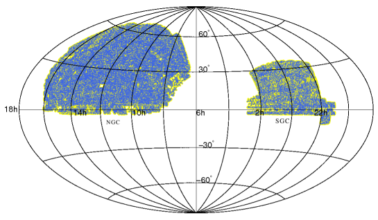
Figure 1: Aitoff projection of the angular distribution of quasars in the final boss sample in equatorial coordinates. The background (yellow) depicts all sectors of the boss survey, as well as a random catalog (for all survey sectors) produced using the bossqsomask software (see the Appendix).The (blue) dots are boss core quasars in survey sectors that have a completeness greater than 75%. The core sample corresponds to objects that have been uniformly-selected using the xdqso algorithm (Bovy et al., 2011).

2 Data

2.1 BOSS Quasars

The sdss-i/ii/iii imaging surveys mapped over 14,000 $\rm{deg^{2}}$ of sky using the sdss camera (Gunn et al., 1998) mounted on a 2.5-meter telescope (Gunn et al., 2006) located at the Apache Point Observatory. Of the unique imaging area released as part of sdss DR8 (Aihara et al., 2011), the boss survey targeted quasars over $\sim 7400\,{\rm deg}^{2}$ of a region around the North Galactic Cap (ngc) and $\sim 2600\,{\rm deg}^{2}$ of a region around the South Galactic Cap (sgc). The Baryon Oscillation Spectroscopic Survey (boss; Dawson et al., 2013), one of four sdss-iii surveys (Eisenstein et al., 2011), has the primary goal of measuring the clustering of luminous red galaxies and neutral hydrogen to determine the cosmic distance scale. As part of this effort, boss measured spectroscopic redshifts of $1.5$ million galaxies and $190{,}000$ quasars using twin multi-object fiber spectrographs (Smee et al., 2013). In this paper, we focus on using these data to measure quasar clustering near $z\sim 2.5$.

boss quasars are selected from point sources in 5-band $ugriz$ imaging (Fukugita et al., 1996) that meet a selection of photometric flag cuts (see the appendixes of Bovy et al., 2011; Ross et al., 2012b) and that fall within magnitude limits of $i>17.8$ and dereddened $g\leq 22.0$ or $r\leq 21.85$. Targeting quasars near $z\sim 2.5$ is difficult, as metal-poor stars typically have colours very close to those of unobscured quasars around redshift 2.7 (e.g., Fan et al., 1999; Richards et al., 2001), and quasars at redshifts of 2.2 to 2.6 can have similar colours to quasars at redshift of about 0.5 because host galaxy light mimics the Lyman-$\alpha$ Forest entering the $u$-band (e.g., Budavári et al., 2001; Richards et al., 2001; Weinstein et al., 2004). These colour similarities are exacerbated near the faint limits of imaging, where flux uncertainties are larger. To circumvent these issues, Bovy et al. (2011) developed the xdqso algorithm to target quasars for boss spectroscopic observation. boss targeted all sources with a ($2.2<z<3.5$) xdqso probability of pqsomidz $>0.424$ tuned to produce 20 deg^-2 quasar targets over the boss footprint (Ross et al., 2012b). This was known as the “core” sample.

The primary mission of the boss quasar survey was to study quasar clustering in the Lyman-$\alpha$ Forest via methods that are insensitive to the quasar selection technique. As such, a heterogeneous range of multi-wavelength data was used to target boss quasars, and a number of methods were incorporated into the survey in addition to xdqso (Richards et al. 2009; Yèche et al. 2010; Kirkpatrick et al. 2011; see Ross et al. 2012b). This heterogeneous or “bonus” approach augmented the core sample.

In this paper we focus on boss quasars spectroscopically confirmed prior to 5th April 2014, which is essentially the final boss quasar compilation. These quasars correspond to boss spectral reduction pipeline version 5-7-0 (spall-v5_7_0). Figure 1 shows the angular distribution of our quasar sample. The yellow background shown in Figure 1 represents the survey area, and the point sources are the core quasars over the redshift range $2.2\leq z\leq 2.8$.

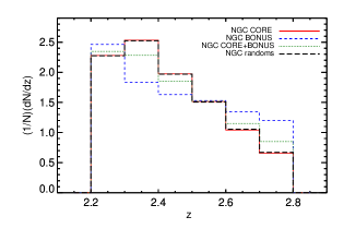
Figure 2: Normalized redshift distributions for the 55,826 ngc-core, 30,551 ngc-bonus and 86,377 ngc-core+bonus quasars over the redshift range $2.2\leq z\leq 2.8$. Also indicated is the redshift distribution generated for the random catalog that is used to mimic ngc-core quasars.

2.2 Targeting Completeness

Quasar clustering measurements are sensitive to the angular completeness of the quasar sample (the “mask”). Quasar spectra in boss were obtained using a set of spectroscopic tiles that can be modeled as polygons using the mangle software (Blanton et al., 2003; Tegmark et al., 2004; Swanson et al., 2008). The fraction of targets (quasars) in an area of the sky that has been covered by a unique set of these tiles (called a sector) is used to define the completeness of the sample. Following White et al. (2012), we limit the survey to sectors with targeting completeness ($f_{\rm comp}$) greater than 75%. About 60% of such sectors are 100% complete, and the mean area-weighted completeness of the sectors we use is $\sim 95$%. A veto mask is applied to remove the regions in which quasars can not be observed such as around bright stars, and near the centerposts of the spectroscopic plates (White et al., 2012).

Note that fiber collisions make it impossible to obtain spectra for quasar pairs closer than 62$\arcsec$ except in overlapping regions (Blanton et al., 2003; White et al., 2012). At the mean redshift of our survey ($\bar{z}\simeq 2.43$), $62\arcsec$ corresponds to a transverse comoving distance of $1.2\,h^{-1}$Mpc. We have not corrected for this fiber collision effect, as it is significant only near the lower edge of the range of scales we consider; this is a region where the errors from shot noise are already quite large.

We adopt the spectroscopic redshift reported by the spectral reduction pipeline spAll-v5_7_0 to compute the comoving distances. To avoid using any target with a problematic redshift, we only accept quasars with zwarning=0, indicating a confident spectroscopic classification and redshift measurement for quasar targets (Bolton et al., 2012).

Unless otherwise specified in the text, we also limit our clustering measurements to just the ngc region of Figure 1, as the ngc represents the largest contiguous area in boss. Excluding the sgc quasars from the original overall core sample of 69,977 quasars significantly affected the clustering signal both in real and redshift space. Previous analyses have also found unexplained differences between clustering measurements in the boss ngc and sgc regions (e.g., White et al., 2012). The target selection papers for the coming eboss survey (Myers et al. 2015, Prakash et al. 2015, in preparation) suggest that the sgc contains areas in which true target density is difficult to regress, which may explain such discrepancies. Table 1 documents how our available sample sizes are affected by restricting to the ngc, to completenesses of $f_{\rm comp}>0.75$, and to zwarning=0.

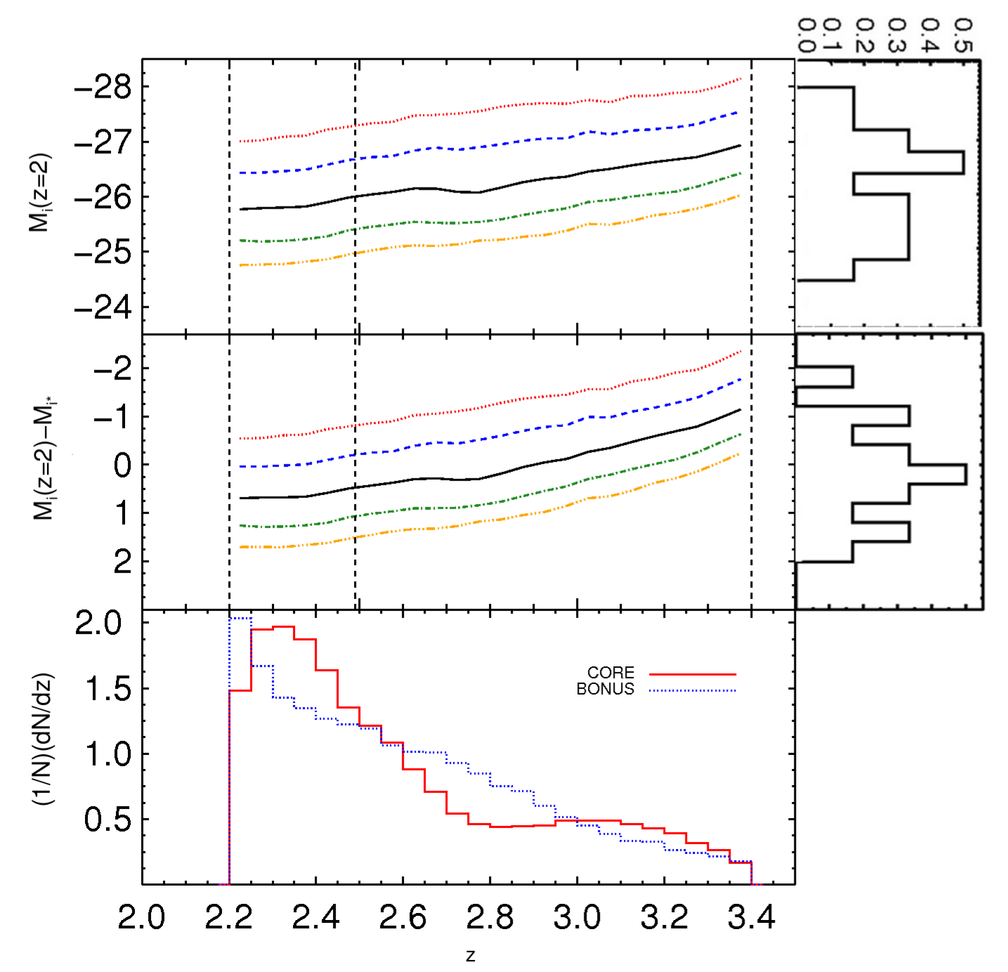
Figure 3: The absolute magnitude distribution for boss quasars. The upper panel displays the $10^{\rm th}$, $25^{\rm th}$, $50^{\rm th}$, $75^{\rm th}$ and $90^{\rm th}$ percentiles of $M_{i}$ vs. redshift. The right-hand side histogram for the upper panel is the normalized distribution of $M_{i}$ for the full ngc-core sample over $2.2\leq z\leq 3.4$. The middle panel shows the same percentiles for $M_{i}-M_{*,i}$ vs. redshift, where $M_{*,i}$ is the characteristic luminosity derived from Eqn. 1. Similar to the upper panel, the right-hand side histogram for the middle panel is the normalized distribution of $M_{i}-M_{*,i}$ for the full ngc-core sample over $2.2\leq z\leq 3.4$. The three vertical dashed lines depict the lower limit, median and the upper limit for the full redshfit range of the samples studied in this paper (2.2, 2.49 and 3.4 respectively). The lower panel is the normalized redshift distribution of quasars over the range $2.2\leq z\leq 3.4$.

Properties	# of quasars
XDQSO targets:
In the core sample	107455
In the bonus sample	104971
Targets with zwarning=0:
In the core sample	103552
In the bonus sample	89044
Targets with $f_{\rm comp}>0.75$ and zwarning=0:
In the core sample	97644
In the bonus sample	79699
ngc core sample	78151
ngc bonus sample	60788
$f_{\rm comp}>0.75$, $2.2\leq z\leq 2.8$:
In the core sample	70892
In the bonus sample	44786
$f_{\rm comp}>0.75$, $2.2\leq z\leq 2.8$, zwarning=0:
In the core sample	69977
In the bonus sample	41019
ngc core sample	55826
ngc bonus sample	30551
$f_{\rm comp}>0.75$, $2.2\leq z\leq 3.4$:
In the core sample	94306
In the bonus sample	60277
$f_{\rm comp}>0.75$, $2.2\leq z\leq 3.4$, zwarning=0:
In the core sample	92347
In the bonus sample	54614
ngc core sample	73884
ngc bonus sample	40781

Table 1: Number of objects in the SDSS DR12 BOSS XDQSO sample with different cuts on redshift and completeness.

2.3 Division by Redshift and Luminosity

To investigate the evolution of quasar clustering, we extended the redshift range by relaxing the upper limit from 2.8 to 3.4 and split the ngc-core sample into three redshift bins that are populated by nearly the same number of quasars (see Table 4). We also check whether the clustering signal is luminosity dependent by dividing the ngc-core sample into three luminosity subsamples based on the absolute magnitude of the quasars in the $i$-band. Following Ross et al. (2013a), we $k$-correct all of our quasar magnitudes to $z=2$. Figure 3 presents the absolute magnitude distribution of the quasars in the final boss ngc-core sample with respect to the characteristic luminosity of quasars at every redshift in this range:

$$M_{i,*}(z)=-21.61-2.5~{}(k_{\rm 1}z+k_{\rm 2}z^{2})-0.71~{},~{}$$ (1)

where $k_{\rm 1}=1.39$ and $k_{\rm 2}=-0.29$ for $z\leq 3$ and $k_{\rm 1}=1.22$ and $k_{\rm 2}=-0.23$ for $z\geq 3$ (from Croom et al. 2004, modified by Croton et al. 2006). Quasars at higher redshift are fainter, and fainter quasars have larger flux uncertainties which translate into imprecision in measured colours. So, at higher redshift the $k$-correction becomes increasingly uncertain. (e.g. Richards et al., 2006).

3 Clustering Measurements and Error Analysis

To determine how much the distribution of quasars deviates from a homogeneous distribution, it is compared to a “random”, or control, set of objects. This random catalog has all of the characteristics of the data, including the selection function, except for its clustering. Figure 2 shows how the redshift distribution of the random catalog we have produced mimics that of the final core boss quasar sample. Appendix A introduces the code that we use to make the random catalog from the survey mask and quasar redshift distribution.

The two-point correlation function $\xi(x)$ is defined as the probability, in excess of random, of finding a pair of objects at a separation $x$: $\delta P=n\delta V[1+\xi(x)]$ (Peebles, 1980). We use the estimator introduced by Landy & Szalay (1993) to calculate the real and redshift-space two-point correlation functions (2PCFs), $\xi(x)$, of quasars in our sample:

$$\xi(x)=\frac{\langle DD(x)\rangle-2\langle DR(x)\rangle+\langle RR(x)\rangle}{\langle RR(x)\rangle},$$ (2)

where $DD(x)$ is the number of data-data pairs with separation between $x$ and $x$+$\Delta x$ and $DR(x)$ is the number of data-random pairs also separated by $x$. The random catalog is constructed to be larger than the data catalog to reduce Poisson noise due to the pair counts that include random points. Consequently, there are normalization factors of the form $N_{\rm R}/N_{\rm D}$ that scale the counts appropriately if the random set has a different size than the data set. The angled brackets denote the suitably averaged pair counts. Throughout this paper we use random catalogs 12 to 20 times larger than our quasar samples. Tests with random catalogs up to 30 times larger than the data show little statistical improvement in the clustering signal, but increase the computing time for our analyses.

Using the comoving distances to each of the two objects in a pair ($s_{1}$ and $s_{2}$), and the angular separation between them ($\theta$), we define each pair’s comoving separation along ($\pi=|s_{1}-s_{2}|$) and across ($r_{\rm p}=[s_{\rm 1}+s_{\rm 2}]\theta/2$) the line of sight. We thus derive the two-dimensional correlation function $\xi(r_{\rm p},\pi)$. Since the effects of redshift space distortions are limited to the line of sight (radial) direction, we can integrate $\xi(r_{\rm p},\pi)$ over $\pi$ in order to eliminate the redshift-space distortion effect:

$$w_{\rm p}(r_{\rm p})=2\int^{\pi_{\rm cut}}_{0}\xi(\pi,r_{\rm p})\rm d\pi,$$ (3)

where the upper limit, ${\pi_{\rm cut}}$, is the distance at which the effects of redshift-space distortions become negligible. We refer to $w_{\rm p}$ as the projected correlation function. Averaging over all pairs whose total redshift-space separation lies in a bin produces the monopole moment of the redshift-space correlation function, $\xi(s)$.

The size, bias and number density of the sample together with the redshift range over which the clustering signal is being measured, can change the optimum value of $\pi_{\rm cut}$. For instance, $70\,h^{-1}$Mpc was used for the 2dF QSO survey of 23,338 quasars (da Ângela et al., 2005), $\sim 100\,h^{-1}$Mpc was used by Shen et al. (2007) for 6,109 quasars at $z\geq 2.9$, and $50\,h^{-1}$Mpc was used for the sample of 27,129 DR10 quasars in the sdss-iii/boss survey (White et al., 2012). The value of $\pi_{\rm cut}$ should be chosen to balance the advantage of integrating out redshift-space distortions against the disadvantage of introducing noise from uncorrelated line-of-sight structure. Moreover, integrating over a wider range of $\pi$ means projecting a larger 3D space into smaller $r_{\rm p}$ bins (e.g., White et al., 2012). After testing a wide enough range of upper limits to truncate the integral, we found $\pi_{\rm cut}=50\,h^{-1}\rm{Mpc}$ to be the optimum limit beyond which the $\xi(r_{\rm p},\pi)$ values become negligible for our sample.

We estimate the uncertainties using inverse-variance-weighted jackknife resampling (Scranton et al., 2002; Zehavi et al., 2002; Myers et al., 2005). We divide our sample into $N$ pixels on the sky, then create $N$ subsamples by neglecting pixels one-by-one and using the remaining area to calculate the 2PCF. We pixelize our sample into angular regions that are specified by HEALPIX pixels (Górski et al., 2005) with $N_{\rm side}=4$ ($\sim 15^{\circ}$ on a side). To compensate for missing areas, we merge pixels with fewer random points than two-thirds of the mean The inverse-variance-weighted covariance matrix elements, $C_{ij}$, are

$$C_{ij}=C(r_{i},r_{j})=\sum^{N}_{L=1}\frac{RR_{L}(r_{i})}{RR(r_{i})}[\omega_{L}(r_{i})-\omega(r_{i})]\\ \times\frac{RR_{L}(r_{j})}{RR(r_{j})}[\omega_{L}(r_{j})-\omega(r_{j})],$$ (4)

where the $L$ subscript refers to the neglected pixel and the random pair ratio, $RR_{L}/RR$, compensates for the relative area through the relative random catalog size in each pixel (e.g Myers et al., 2007a). One-standard-deviation jackknife errors, $\sigma_{i}$, are the square root of the diagonal elements of the covariance matrix. We assume the errors are Gaussian, and thus compute the goodness-of-fit or likelihood of any model that fitted to the data through

$$\chi^{2}=\sum_{i,j}\left[w(r_{i})-w_{\rm model}(r_{i})\right]C^{-1}_{ij}\left[w(r_{j})-w_{\rm model}(r_{j})\right].$$ (5)

4 Clustering Results

4.1 Real-space correlation function

To measure the projected auto-correlation function $w_{\rm p}(r_{\rm p})$ we use a sample of 55,826 ngc-core quasars within the redshift range $2.2\leq z\leq 2.8$ (see Table 1).

For sufficiently large $\pi_{\rm max}$, $w_{\rm p}(r_{\rm p})$ can be related to the real-space clustering as (Davis & Peebles, 1983)

$$w_{\rm p}(r_{\rm p})=2\int^{\infty}_{r_{\rm p}}\frac{r\xi(r)}{\sqrt{r^{2}-r^{2}_{\rm p}}}{\rm d}r.$$ (6)

As a first model, we use a simple power law of the form ($r/r_{\rm 0})^{-\gamma}$ for the real-space correlation function. For this power-law form, Eqn. 6 reduces to

$$\frac{w_{\rm p}(r_{\rm p})}{r_{\rm p}}=\frac{\sqrt{\pi}~{}\Gamma[(\gamma-1)/2]}{\Gamma[\gamma/2]}\left(\frac{r_{\rm 0}}{r_{\rm p}}\right)^{\gamma}.$$ (7)

We approach the fitting process in two separate ways:

(1) First, we perform a two-parameter fit using the $\chi^{2}$ minimization method to determine both the slope and the intercept of the fitted line. We use the resulting slope ($\gamma\sim 1.85$) as a fixed parameter and perform a one-parameter $\chi^{2}$ minimization, obtaining a scale length of $\rm r_{0}=7.7\pm 0.2\,h^{-1}{\rm Mpc}$ with $\chi^{2}_{\rm red}=0.36$ over 9 degrees of freedom.

(2) Second, we fix $\gamma=2$ and fit a 1-parameter model. This allows us to evaluate how much clustering amplitude is sensitive to the chosen slope of the model. This fit results in a scale length of $r_{\rm 0}=8.12\pm 0.22\,h^{-1}{\rm Mpc}$ with $\chi^{2}_{\rm red}=0.25$ over 10 degrees of freedom.

Since a slight change in the slope does not make a significant difference to the result of the fit for the clustering amplitude, we conclude that the clustering amplitude for our quasar sample in the fitted range is not strongly sensitive to the slope of the real-space correlation function. As we find that $\gamma=2$ is an acceptable value of the slope, we proceed by using $\gamma=2$ throughout the rest of this paper so that our fitted correlation lengths can be compared more easily to other works (e.g Shen et al., 2007; White et al., 2012).

Fig. 4 presents the results of the fits to the measured $w_{\rm p}$. The fitting range in both approaches is $4\lesssim r_{\rm p}\lesssim 25\,h^{-1}{\rm Mpc}$. We find that $\chi^{2}$ maintains an acceptable level, and that our fitting results are consistent within the derived uncertainties, for all fitting ranges from $4\lesssim r_{\rm p}\lesssim 16\,h^{-1}{\rm Mpc}$ to $2\lesssim r_{\rm p}\lesssim 50\,h^{-1}{\rm Mpc}$. An improved mask and/or deeper imaging for the initial target selection of rare and faint high-redshift quasars would be needed to push the fitting scales further in order to measure subtle large-scale features, but the quasar bias measurement should be well characterized over the moderate scales of $<25\,h^{-1}\rm Mpc$.

$r_{\rm p}$	4.36	5.18	6.15	7.31	8.69	10.33	12.28	14.59	17.34	20.61	24.50
$w_{\rm p}$	54.64	48.87	43.41	38.09	29.77	26.47	22.74	16.68	11.90	15.27	7.80
$\sigma$	12.45	9.45	9.56	8.64	5.68	5.88	4.17	3.44	3.16	3.01	3.09
4.36	1.000	-0.256	-0.052	-0.343	0.027	0.485	0.221	0.171	0.174	0.553	0.543
5.18	-	1.000	0.023	0.152	0.455	-0.215	0.320	-0.298	-0.299	-0.245	-0.241
6.15	-	-	1.000	0.232	-0.119	-0.379	-0.083	-0.225	-0.261	-0.419	-0.273
7.31	-	-	-	1.000	0.083	-0.410	0.095	-0.050	-0.958	-0.606	-0.579
8.69	-	-	-	-	1.000	0.472	0.202	0.153	0.656	0.538	0.529
10.33	-	-	-	-	-	1.000	0.484	0.382	0.388	0.138	0.119
12.28	-	-	-	-	-	-	1.000	0.031	0.035	-0.166	0.154
14.59	-	-	-	-	-	-	-	1.000	0.004	0.323	0.309
17.34	-	-	-	-	-	-	-	-	1.000	0.320	0.306
20.61	-	-	-	-	-	-	-	-	-	1.000	0.083
24.50	-	-	-	-	-	-	-	-	-	-	1.000

Table 2: Correlation coefficients as estimated from the covariance matrix computed by jackknife error estimation for ngc-core quasars. The first three rows are the comoving separation, $r_{\rm p}$ (in $h^{-1}{\rm Mpc}$), the auto-correlation $w_{\rm p}$ and its uncertainty. The remainder of the table lists the correlation coefficients as estimated from the covariance matrix computed by jackknife error estimation.

Using the method described in $\S$3, we estimate the covariance matrix of the auto-correlation function (ACF) for ngc-core quasars. The $w_{\rm p}$ result for the ACF of the ngc-core quasar sample over the fitting range $4<r_{\rm p}<25\,h^{-1}{\rm Mpc}$ and its uncertainty ($\sigma$) are reported in the first three rows of Table 2. The remainder of the table lists the correlation coefficients as estimated from the covariance matrix calculated via inverse-variance-weighted jackknife resampling.

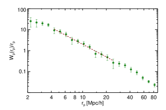
Figure 4: The projected auto-correlation function for the core sample over the redshift range $2.2\leq z\leq 2.8$. The dashed line is the best-fit one-parameter power law over the range $4<r_{\rm p}<25\,h^{-1}{\rm Mpc}$. Because the two-parameter power-law fit does not have a significantly different slope to the one-parameter power-law over the chosen fitting range, we adopt $\gamma=2$ throughout this paper for consistency with White et al. (2012).

4.2 Using boss bonus quasars

As mentioned in $\S$2, boss also surveyed a heterogeneously selected quasar sample with a complicated angular selection function—the bonus sample. Although modeling the mask for the bonus sample is beyond the scope of this paper, we can cross-correlate a bonus+core sample against the core sample, using the random catalog constructed for the core sample, in an attempt to improve our measurement precision. Expanding the main sample by adding quasars from the bonus sample might be expected to improve the clustering signal (as there are more total pair counts in a core+bonus-to-core cross correlation than in a core-to-core ACF) but it is worth determining whether such an approach is justified by improved statistics.

Fig. 5 shows the cross-correlation of core+bonus (86,377 quasars) against core (55,826 quasars) for objects in the ngc with zwarning=0 and completeness greater than 75$\%$. For the cross-correlation estimator, the “DD” pairs in Eqn. 2 consist of one member from the core and another from the core+bonus sample. The random catalogue, here, was made for the uniformly selected (i.e. core) sample, so the “2DR” pair breaks into a “DR” pair for the core and a “DR” pair from the core+bonus sample, where ”R” always denotes the random catalog constructed for the CORE sample. In other words, Eqn. 2 for the cross-correlation estimator that we adopt is $\xi(x)=(\langle D_{C}D_{CB}(x)\rangle-\langle D_{C}R(x)\rangle-D_{CB}R(x)+\langle RR(x)\rangle)/\langle RR(x)\rangle$, where the subscripts “c” and “cb” refer to the core and core+bonus samples respectively. The appropriate data/random normalization factors are included here (as in the description of Eqn. 2).

The difference between the ACF and cross-correlation at every scale is well within the $1\sigma$ uncertainty. However, the cross correlation has slightly better precision on smaller scales, which would be a benefit to measurements of, e.g., the one-halo term in the HOD formalism. The consistency of the clustering replacing the ACF with a cross correlation is a useful check on our analyses, and may also represent one way forward for performing clustering measurements using heterogeneous samples. However, given the only minor improvement, we continue using the ACF throughout this paper.

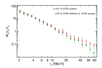
Figure 5: Projected cross-correlation between the 55,826 core and 86,377 core+bonus quasars over the redshift range $2.2\leq z\leq 2.8$ (red open circles). The cross-correlation result is consistent with the auto-correlation of the core sample (green filled circles) over our scales of interest. As little additional precision is introduced by using the full core+bonus sample, we restrict our analysis to just the auto-correlation of the core sample.

$r_{\rm p}$	$w_{\rm p}$	$\sigma$	$w_{\rm p}$	$\sigma$	$s$	$\xi(s)$	$\sigma$
$(h^{-1}{\rm Mpc})$	ACF		CCF		$(h^{-1}{\rm Mpc})$
2.09	69.353	19.294	73.474	17.498	3.06	2.556	0.609
2.53	60.807	14.491	64.523	13.311	3.70	1.663	0.384
3.06	57.125	10.707	63.607	10.438	4.48	2.406	0.318
3.70	52.908	8.654	58.216	8.133	5.41	1.654	0.213
4.47	45.454	5.981	46.928	5.365	6.55	1.020	0.132
5.41	39.291	10.607	36.604	11.831	7.92	1.034	0.101
6.55	34.392	9.142	33.677	9.015	9.59	0.676	0.069
7.92	25.846	6.051	28.909	6.567	11.60	0.562	0.050
9.58	23.907	5.210	27.066	5.061	14.03	0.433	0.036
11.60	16.056	3.002	19.692	3.129	16.97	0.291	0.026
14.03	11.771	1.854	16.066	3.196	20.54	0.193	0.018
16.97	13.753	5.348	18.433	8.045	24.84	0.150	0.014
20.54	9.404	3.130	13.768	5.087	30.06	0.090	0.010
24.85	6.824	0.958	9.8349	3.872	36.37	0.069	0.007
30.06	6.554	2.099	10.018	3.256	43.10	0.040	0.006
36.37	7.341	1.422	10.170	2.184	53.23	0.020	0.004
44.00	4.192	1.061	8.122	5.365	64.40	0.010	0.003
53.23	4.483	1.076	8.535	3.208	77.92	-0.000	0.002
64.40	2.576	0.159	6.711	3.004	94.27	0.004	0.002

Table 3: Projected and redshift-space correlation functions. ACF $w_{\rm p}$ represents the auto-correlation of the ngc-core sample, CCF $w_{\rm p}$ is the cross-correlation between the ngc-core+ngc-bonus and ngc-core samples and $\xi(\rm s)$ is the redshift-space correlation for ngc-core quasars over the redshift range $2.2\leq z\leq 2.8$.

4.3 Redshift-space 2-point correlation function

Using redshift to infer distance for the 2PCF causes a complication; peculiar velocities introduce redshift-space distortions in $\xi$ along the line of sight (Kaiser, 1987). This effect has utility, though, as measuring these redshift space distortions can constrain cosmological parameters.

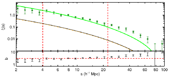
Figure 6: The redshift-space correlation function $\xi(s)$ for 55,826 boss ngc-core quasars over the redshift range $2.2\leq z\leq 2.8$. The black curve is the real-space correlation function, $\xi(r)$ of dark matter from halofit (Smith et al., 2003) modified by the correction for redshift space distortions from Kaiser (1987). The resulting best-fit bias (green curve) is $b_{\rm Q}$ = 3.54. The lower panel depicts the bias residuals compared to the fiducial fit. The (red) vertical dashed lines at $\sim 4\,h^{-1}\rm Mpc$ and $\sim 22\,h^{-1}\rm Mpc$ depict the scale over which we fit the data.

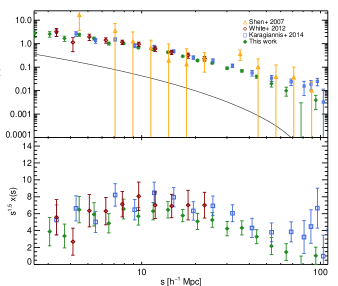
Figure 7: Comparison of our redshift-space correlation function with earlier works. White et al. (2012) and Karagiannis, Shanks & Ross (2014) both used samples of $\sim 25{,}000$ core quasars from boss over the same redshift range we consider in this paper ($2.2\leq z\leq 2.8$). Shen et al. (2007) used $\sim$4,400 quasars from sdss Data Release 5 over $2.9\leq z<5.4$. The black curve is as for Fig. 6.

Fig. 6 shows the redshift-space correlation function $\xi(s)$ of 55,826 ngc-core quasars over the redshift range 2.2 $\leq z\leq$ 2.8. As described in $\S$3, a jackknife resampling is used to derive both the uncertainties and the full covariance matrix. The black curve is the real-space correlation function, $\xi(r)$ of dark matter computed from halofit (Smith et al., 2003) modified by the relationship between the redshift-space and real-space correlation functions (Kaiser, 1987)

$$\xi(s)=\left(b^{2}+\frac{2}{3}bf+\frac{f^{2}}{5}\right)\xi(r),$$ (8)

where $f=[\Omega_{m}(z)]^{0.56}$ is the gravitational growth factor. The model is then fit to the measured correlation function for quasars by $\chi^{2}$ minimization. The best-fit bias of quasars relative to the underlying dark matter is $b_{Q}$ = 3.54 $\pm$ 0.1 with $\chi^{2}_{\rm red}=1.06$ for 7 degrees of freedom using the full covariance matrix. The lower panel of Fig. 6 presents the bias residuals and the horizontal dashed line represents the best-fit value of the bias. The vertical dashed line indicates the edge of the last bin that is included in the fit. This figure demonstrates that scale-independent bias combined with a $\Lambda$CDM cosmology is a sufficient fit to our data over scales of at least $4\lesssim s\lesssim 22\,h^{-1}{\rm Mpc}$.

Table 3 presents our measurements of the projected auto-correlation function and redshift-space auto-correlation function, as well as the projected cross correlation with bonus quasars (see §4.2). The reported uncertainties for all correlation functions are the diagonal elements of the covariance matrix derived by inverse-variance-weighted jackknife resampling. Our result for the redshift-space correlation function is compared to other works in Fig. 7. The figure shows some consistency between previous results, although our work is in better agreement with a $\Lambda$CDM cosmology on large scales.

In general, the excess of the data above the model seen by ourselves and other authors for scales greater than $\sim 25\,h^{-1}{\rm Mpc}$ is likely to be due to the difficulty in building a random catalog that fully mimics complex and subtle deviations in target density that manifest on large scales where the correlation amplitude is small (e.g., Ross et al., 2011; Ho et al., 2015). Notably, Agarwal et al. (2014) demonstrate that unknown systematics can affect quasar clustering amplitude on very large scales. The disagreement between our adopted model and the data on scales of $s>27\,h^{-1}{\rm Mpc}$ is likely to be due to the very small error bars on these scales being driven by correlations in imaging systematics, which, when jackknifed, lead to an underestimate of the true errors. Weighting the target density using systematics maps to see if the clustering fit can be pushed to larger scales is currently under investigation, but is beyond the scope of this paper. CDM is known to be a good description of underlying dark matter and, therefore, in this work, we focus on deriving the quasar clustering amplitude and slope for the scales on which CDM represents a good fit, and on which we therefore believe our data to be uncontaminated by subtle systematics.

4.4 2-D Redshift-space correlation function, $\xi(r_{\rm p},\pi)$

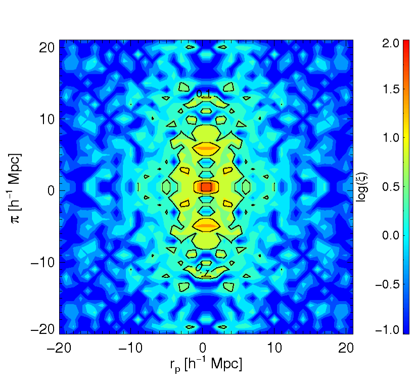
Figure 8: The two-dimensional redshift-space correlation function $\xi(r_{\rm p},\pi)$ for 55,826 ngc-core boss quasars. The extension in the line-of-sight direction is due to a combination of redshift errors and “Fingers-of-God”.

As mentioned in $\S$3, one can project the redshift space separation between two objects into orthogonal components along ($\pi$) and across ($r_{\rm p}$) the line of sight. The elongation of virialized overdensities such as clusters of galaxies along the line of sight, caused by small peculiar velocities that are not associated with the Hubble flow, should be visible in 2-D redshift-space maps as long, narrow filaments aligned with the line of sight (Tegmark et al., 2004). To check whether this “Fingers of God” effect is apparent in our sample, we measure $\xi(r_{\rm p},\pi)$ for our ngc-core quasars out to scales of $\pm 20\,h^{-1}\rm Mpc$, and display the results in Fig. 8. It is clear from Fig. 8 that the redshift-space distortions are strongest for $\pi<20\,h^{-1}\rm{Mpc}$, confirming that our adopted redshift-space integration limit of $\pi_{\rm cut}=\pm 50\,h^{-1}\rm{Mpc}$ is reasonable. Although we choose not to further analyze $\xi(r_{\rm p},\pi)$ in this paper, Fig. 8 implies that studies of redshift-space distortions would be a meaningful avenue for further cosmological studies using boss quasars.

5 Evolution and luminosity dependence of quasar clustering

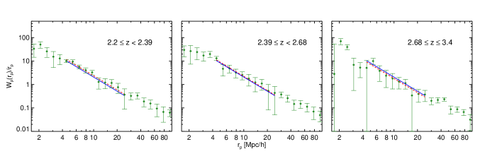
Figure 9: The projected real-space clustering of the ngc-core sample in three bins of redshift containing roughly equal numbers of quasars. See Table 4 for the sample properties and Table 5 for the fitting results. The red dashed line is the one-parameter fitted power-law with $\gamma=2.0$ and the blue solid line is the one-parameter fitted power-law to the measured correlation function of the main sample plotted here as a reference line.

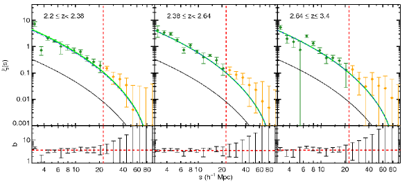
Figure 10: The measured redshift-space correlation function $\xi(s)$ for the three redshift subsamples detailed in Table 4. The fitting range for all three subsamples is $3.0\lesssim s\lesssim 22.5\,h^{-1}\rm Mpc$ and the fitting results are detailed in Table 5. The green curve is the fitted dark matter correlation function to the measured $\xi(s)$ for each sample and the overlaid blue dashed curve is the fitted curve to the $\xi(s)$ for the main sample, plotted here as a reference for comparison.

$\Delta z$	$\bar{z}$	# of	# of ngc	n$~{}(10^{-6})$
		quasars	quasars	$(h^{-1}\rm Mpc)^{-3}$
$2.20\leq z<2.39$	2.297	30824	24667	$4.283\pm 0.027$
$2.39\leq z<2.64$	2.497	30707	24493	$3.001\pm 0.019$
$2.64\leq z\leq 3.40$	2.971	30816	24724	$1.057\pm 0.007$

Table 4: Properties of the three core subsamples over the redshift range $2.2\leq z\leq 3.4$. The columns are redshift range, average redshift and total number of quasars for each redshift subsample with or without sgc quasars. The final column is the number density of the NGC quasars in each subsample, together with Poisson errors.

5.1 Redshift dependence

In order to have sufficient dynamic range to characterize the evolution of quasar clustering, we extend the redshift upper limit we study from 2.8 to 3.4. We divide the resulting sample of 73,884 ngc-core quasars into three subsamples and measure the projected 2PCF both in real and redshift space for each subsample. Table 4 summarizes the properties of the three redshift subsamples. The dividing redshifts (2.384 and 2.643) were selected such that the three subsamples contain almost the same number of quasars.

Fig. 9 shows the result of measuring the real-space 2PCF as a function of redshift. Motivated by the fitting result of the ngc-core sample described in $\S$4.1, we fit a power law of index $\gamma=2$ over scales of $4\lesssim r_{\rm p}\lesssim 25\,h^{-1}\rm Mpc$ for each of the three redshift bins. The scatter of the points (10 points are included in the fit for each 2PCF) results in higher uncertainties on the best-fit correlation length—but $r_{0}$ remains similar as a function of redshift.

To evaluate how much fixing the power-law index affects our results, we allow $\gamma$ to float as a second free parameter in the fit over the same range. There is a considerable difference between the assumed $\gamma=2.0$ and the best-fit value for some redshift bins ($\gamma_{1}=1.57\pm 0.12$, $\gamma_{2}=1.69\pm 0.37$ and $\gamma_{3}=1.88\pm 0.29$). However, the best-fit values for $r_{0}$ remain consistent within the error bars.

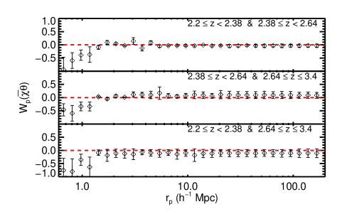
Figure 11: The one-dimensional projected cross-correlation function $\rm w_{p}(\bar{\chi}\theta)$ between quasars in different redshift subsamples. Lack of any strong correlation between redshift subsamples demonstrates that our masking procedure and pipeline-based redshift determinations are robust over our fitting scales. We measure only the coordinate transverse to the line-of-sight ($r_{\rm p}$), as different redshift bins are correlated along the line-of-sight. The data deviate from the from the dashed line (zero correlation) for scales below $\sim 1.5\,h^{-1}\rm Mpc$; we discard these points for all of the fits. This deviation is most likely caused by the fact that boss can not place fibers at separations smaller than 62″ ($1.3\,h^{-1}\rm Mpc$ at $z=2.5$) on a single plate. We note that the slight deviations ($<\pm 0.1$) from zero at scales of $>1.5\,h^{-1}\rm Mpc$ in the lower two panels are insignificant given the high covariance of the data on different scales. Nevertheless, these deviations could indicate low-level, correlated substructure in our masks that might, e.g., depend on how the depth of the quasar target sample changes with redshift.

$\Delta z$	$\Delta M_{i}$	$\bar{z}$	# of quasars	$\rm b_{Q}$	$\chi^{2}_{\rm red}$	$\rm r_{0}$($h^{-1}\rm Mpc$)	$\chi^{2}_{\rm red}$
$2.20\leq z\leq 2.80$	$-28.74\leq M_{i}\leq-23.78$	2.434	55826	3.54 $\pm$ 0.10	1.06	8.12 $\pm$ 0.22	0.25
$2.20\leq z<2.384$	$-28.70\leq M_{i}\leq-23.95$	2.297	24667	3.69 $\pm$ 0.11	1.55	8.68 $\pm$ 0.35	0.45
$2.384\leq z<2.643$	$-28.74\leq M_{i}\leq-24.11$	2.497	24493	3.55 $\pm$ 0.15	0.61	8.42 $\pm$ 0.54	0.26
$2.643\leq z\leq 3.40$	$-29.31\leq M_{i}\leq-24.40$	2.971	24724	3.57 $\pm$ 0.09	0.66	7.59 $\pm$ 0.66	0.33
$2.20\leq z\leq 2.80$	$-28.74\leq M_{i}<-26.19$	2.456	18477	3.69 $\pm$ 0.10	2.19	8.62 $\pm$ 0.27	0.94
$2.20\leq z\leq 2.80$	$-26.19\leq M_{i}<-25.36$	2.436	18790	3.56 $\pm$ 0.13	1.71	7.94 $\pm$ 0.41	1.63
$2.20\leq z\leq 2.80$	$-25.36\leq M_{i}\leq-23.78$	2.411	18559	3.81 $\pm$ 0.19	0.4	8.29 $\pm$ 0.36	3.29

Table 5: Clustering results for ngc-core sample and subsamples. The first five columns are redshift and absolute magnitude range, their average values and the total number of NGC quasars in each of the luminosity and redshift subsamples. Columns 6, 7 and 8 are the bias values that best fit our measured redshift-space correlation function, their uncertainty and the reduced $\chi^{2}$ (over 7 degrees of freedom for the main sample and 9 degrees of freedom for the redshift and luminosity subsamples). Column 9 is the best fit correlation length which is the result of fitting a one parameter power-law with a fixed index of 2.0 to the measured real-space correlation function of quasars in each subsample. The last two columns are the uncertainty on the correlation length and its reduced $\chi^{2}$ (over 8 degrees of freedom for the redshift and luminosity subsamples and over 9 degrees of freedom for the main sample). The lower limits on $\Delta M_{i}$ for the redshift subsamples and full samples are the highest luminosity quasars that happen to occur in the sample and no imposed upper limit in the selection is applied.

We measure the redshift-space correlation function for the same three redshift-based subsamples. Similar to our approach for the real-space correlation function, we fit $\xi(s)$ for the three subsamples over the same fitting range as $\xi(\rm s)$ for the full ngc-core sample and measure the bias of quasars relative to dark matter in every bin of redshift. Fig. 10 displays $\xi(s)$ for the three subsamples. The model represented by the solid curve is as for Fig. 6. Lower number densities for quasars in the subsamples produce noisier covariance matrices. As a result, we only use the diagonal elements of those matrices when fitting the real- and redshift-space correlation functions.

The upper part of Table 5 displays the fitting results for the evolution of the real and redshift-space correlation functions. Including full covariance matrices in our fits increases $\chi^{2}$ without producing a meaningful change in the best-fit value for the bias. The covariance matrices for $\xi$ are less noisy than for $w_{\rm p}$ on larger scales—but extending the fits to larger scales for $\xi(s)$ (beyond the vertical dashed lines in Fig. 6 and Fig. 10), still results in a large increase in uncertainty for the best-fit bias, presumably because the larger scale measurements are not well fit by the same bias factor and $\Lambda$CDM model that fits the data at $s\la 25\,h^{-1}\rm Mpc$.

As a further test of our overall masking procedures, we calculate the cross-correlation function between quasars in different bins of redshift and display the results in Fig. 11. The lack of any strong correlation between different redshift subsamples demonstrates that the pipeline-based redshifts used for this study are of sufficient reliability and that the masking procedure we use to produce the angular selection function for boss quasars is robust.

There have been few measurements of quasar clustering near $z\sim 2.5$, which indicates the difficulties inherent in uniformly-selecting large numbers of quasars near this redshift. Fig. 12 and Fig. 13 show the reported values of correlation length and quasar bias from previous works (Porciani, Magliocchetti & Norberg, 2004; Croom et al., 2005; da Ângela et al., 2005; Myers et al., 2006; Porciani & Norberg, 2006; Myers et al., 2007a; Shen et al., 2007; da Ângela et al., 2008; Ross et al., 2009; White et al., 2012; Font-Ribera et al., 2013).

Some caution is required in interpreting Figures 12 and 13, as different samples probe different luminosity ranges and different groups have made different assumptions and choices when inferring $r_{0}$ and bias (e.g., power-law vs. $\Lambda$CDM fit, projected or redshift-space fit, range of separations used) and when computing the error bars on their results. For Figure 13, we have corrected all bias values to our adopted cosmology by multiplying the authors’ reported values and error bars by $\sigma_{8,{\rm rep}}(z)/\sigma_{8,{\rm fid}}(z)$ where $\sigma_{8,{\rm rep}}(z)$ is the value of $\sigma_{8}$ at redshift $z$ in the reported cosmology and $\sigma_{8,{\rm fid}}(z)$ is the value for our fiducial cosmology (see §1). Shen et al. (2007) report values of $r_{0}$ for samples in “all fields” and “good fields” (with higher photometric data quality but a smaller sample) at effective redshifts $z=3.1$ ($2.9\leq z\leq 3.5$) and $z=4.0$ ($z\geq 3.5$). For corresponding bias values in Figure 13 we use those calculated by White, Martini & Cohn (2008) by fitting the Shen et al. measurements.

The BOSS measurements of quasar bias, from this paper and from the Ly$\alpha$ forest cross-correlation measurement of Font-Ribera et al. (2013), are the most precise constraints at any redshift, and by far the most precise at $z>2$. Our value of $b_{Q}=3.54\pm 0.10$ for the redshift range $2.2\leq z\leq 2.8$ is compatible with Font-Ribera et al.’s value of $3.64^{+0.13}_{-0.15}$ at $1\sigma$, a reassuring level of consistency given the difference of measurement methods. Our bias and $r_{0}$ values are higher than most of those measured at $z<2$, though these are typically for lower luminosity thresholds so it is difficult to separate redshift and luminosity effects. Our redshift subsample measurements are consistent with constant $r_{0}$ or constant bias over the redshift range $2.2\leq z\leq 3.4$. (Because matter clustering grows by a factor of 1.35 over this redshift span, constancy of one quantity implies evolution of the other, but our measurement errors are too large to definitively establish evolution of either.) The SDSS-based measurements of Shen et al. (2007) are significantly higher than ours. We discuss the marked difference between our measurements and the Shen et al. (2007) value at $z=3.1$ ($b_{Q}=6.9\pm 0.7$ for “all fields”) in §6.

$\Delta M_{i}$	$\bar{M}_{i}$	# of	# of ngc	n$~{}(10^{-6})$
		quasars	quasars	$(h^{-1}\rm Mpc)^{-3}$
$[-28.74,-26.19]$	-26.87	23809	18477	$0.982\pm 0.0072$
$[-26.19,-25.36]$	-25.77	23669	18790	$0.998\pm 0.0073$
$[-25.36,-23.78]$	-24.90	22499	18559	$0.986\pm 0.0072$

Table 6: Properties of the three ngc-core absolute magnitude subsamples over the redshift range $2.2\leq z\leq 2.8$. The columns list the absolute magnitude range and its average for each luminosity subsample as well as the total number of quasars in each subsample with or without sgc quasars (3rd and 4th columns respectively). $\bar{M}_{i}$ corresponds to the average absolute magnitudes of the ngc quasars in each subsample. The last column is the number density and the Poisson errors of the quasars in each subsample.

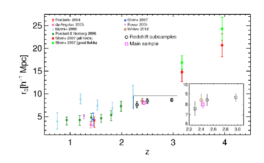
Figure 12: Evolution of the correlation length $r_{\rm 0}$ with redshift. We display the results for all ngc-core quasars (open orange square) and for the different redshift ranges (open black circles) and absolute magnitude bins (filled black triangles) studied in this work (see Table 5). Results from prior works have been recalibrated to reflect our chosen cosmology. The inset provides a more detailed view of the range $2.2\leq z\leq 3.0$.

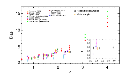
Figure 13: Evolution of quasar bias with redshift. We display the results for all ngc-core quasars (open orange square) and for the different redshift ranges (open black circles) and absolute magnitude bins (filled black triangles) studied in this work (see Table 5). Results from prior works have been recalibrated to reflect our chosen cosmology. The inset provides a more detailed view of the range $2.2\leq z\leq 3.0$.

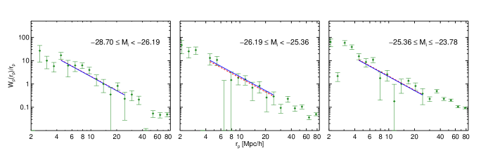
Figure 14: To constrain any luminosity dependence of the clustering of boss quasars, we divide the quasar sample into three absolute magnitude subsamples covering the same redshift range ($2.2\leq z\leq 2.8$). The three panels display the real space-correlation function fitted by a one-parameter power law over scales of $4\lesssim r_{\rm p}\lesssim 25\,h^{-1}{\rm Mpc}$. The red dashed line is the one-parameter fitted power-law with $\gamma=2.0$ and the blue solid line is the one-parameter fitted power-law to the measured correlation function of the main sample plotted here as a reference line.

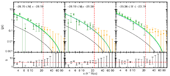
Figure 15: Similar to Fig. 10 but for samples in the redshift range $2.2\leq z\leq 2.8$, subdivided by absolute magnitude. See Table 5 for the fitting results. The green curve is the fitted dark matter correlation function to the measured $\xi(s)$ for each sample and the overlaid blue dashed curve is the fitted curve to the $\xi(s)$ for the main sample, plotted here as a reference for comparison.

5.2 Luminosity dependence

As described in §2.3, we divide the ngc-core sample of 55,826 quasars into three luminosity subsamples (see Table 6), such that there is a distinct difference between the average luminosity for each equally sized subsample. Fig. 14 and Fig. 15 present the results of measuring the real and redshift-space correlation functions, respectively, for these luminosity-based subsamples. As the luminosity subsamples have even lower number densities than the redshift subsamples, the covariance matrices for the luminosity-based ACFs are noisier than those for the redshift subsamples, so we fit their real- and redshift-space correlation functions using only the diagonal elements of their covariance matrices. An assumption of diagonal error covariance may be fairly accurate for these sparse samples, as shot noise makes a large contribution to the error budget.

Figure 16 shows the dependence of $r_{0}$ and $b$ on luminosity for these three subsamples, each with an effective redshift $z\approx 2.4.$ Because of the difference between fitting a power-law (for $r_{0}$) and a $\Lambda$CDM correlation function (for $b$), the order of points is not the same in the two panels, but it is clear that the data are consistent with constant $r_{0}$ or $b$, independent of luminosity over our measured range. Solid curves show power-law fits of the form $a(L/L_{0})^{m}$ for which we find $m=0.56\pm 0.80$ (for $r_{0}$) or $m=-0.027\pm 0.27$ (for $b$), consistent with $m=0$. Dashed horizontal lines show the best fit with $m$ forced to zero. Our highest luminosity sample has a threshold $M_{i}<-26.19$ vs. $M_{i}<-26.6$ for Shen et al. (2007). The lack of either redshift or luminosity trends within our sample therefore makes the significantly higher clustering of their sample (spanning $2.9\leq z\leq 3.5$) somewhat surprising. However, we have not attempted to measure clustering for a sample that mimics both their redshift range and luminosity threshold.

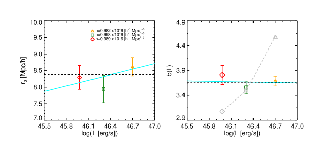
Figure 16: The variation of the measured correlation length and measured and expected bias as a function of bolometric luminosity for quasars in three absolute magnitude subsamples. Each of the luminosity subsamples has a similar redshift ($z=2.456$, $z=2.436$ and $z=2.411$). The number density of quasars in each sample ($n$) is recorded in the legend of the left-hand panel. The blue solid line is the best-fit power law (in the general form of $a(L/L_{0})^{m}$ with $\rm log_{10}(L_{0})=46.33$) to the measured correlation length and bias values in the three luminosity bins. The black dashed line is the best-fit power law with $m=0$ (i.e. a model for which clustering does not depend on luminosity). In the right-hand panel, the coloured symbols are the best fit biases to the measured $\xi(s)$ for each sample. The slopes of the fitted line to the measured (coloured) biases and correlation lengths are $m=-0.027\pm 0.27$ and $m=0.56\pm 0.80$ respectively. The connected grey points in the right hand panel show the predicted luminosity dependence of bias if quasar luminosity is monotonically related to halo mass and all halos have the same quasar duty cycle $f=0.0073$ that best fits the full sample.

6 Halo Masses and Duty Cycles

Following the approach proposed in a range of previous works (e.g. Haiman & Hui, 2001; Martini & Weinberg, 2001; Wyithe & Loeb, 2005), we now use our clustering measurements to constrain the host halo masses of BOSS quasars and the duty cycles of quasar activity in these halos. The constraint on halo mass comes from the fact that more massive halos have higher clustering bias (Kaiser, 1984; Tinker et al., 2010), so the observed clustering of quasars determines the characteristic mass of their host halos. Moving from this halo mass to a duty cycle requires a further assumption to relate luminosity and halo mass. Here we assume that this relation is monotonic with no scatter—the black hole in a given halo is either “on” (i.e. observed as a quasar) or “off”—and we test whether this assumption is consistent with our observed (lack of) luminosity dependence.

For each of our samples we compute both a characteristic halo mass ${\bar{M}_{h}}$ and a minimum halo mass ${M_{h,\rm min}}$ (see Table 7). We calculate these values using the formula of Tinker et al. (2010) to model $b(M)$. Specifically, we use their Eqn. 6 with parameters chosen for an overdensity of $\Delta=200$ and with our adopted cosmology. We quote a characteristic mass as, simply, the mass that corresponds to our measured bias in the Tinker et al. (2010) formalism (i.e. $b_{Q}=b({\bar{M}_{h}})$). Alternatively, in our adopted model, ${M_{h,\rm min}}$ can be determined from the range of halos that correspond to a given bias measurement via

$$b(M>M_{h,{\rm min}})\equiv\frac{\int_{M_{h,{\rm min}}}^{\infty}\frac{dn}{dM}b(M)dM}{\int_{M_{h,{\rm min}}}^{\infty}\frac{dn}{dM}dM}$$ (9)

i.e. our measured bias $b_{Q}=b(M>{M_{h,\rm min}})$ is then interpreted to be the mean bias of halos with mass above ${M_{h,\rm min}}$ weighted by the halo abundance $dn/dM$, which we take from the Tinker et al. (2008) halo mass function at the mean redshift appropriate to each of our samples (see Table 5).

Associating ${M_{h,\rm min}}$ with the minimum halo mass required to host a quasar above the sample luminosity threshold implicitly assumes that all halos above ${M_{h,\rm min}}$ have an equal probability of hosting a sample quasar (i.e. constant duty cycle) and that halos below ${M_{h,\rm min}}$ can only host quasars below the luminosity threshold (i.e. quasars hosted in halos below a threshold of ${M_{h,\rm min}}$ are not present in our sample).

We determine ${\bar{M}_{h}}$ and ${M_{h,\rm min}}$ and their errors by matching the best-fit values and error range of $b_{Q}$ recorded in Table 5 and report these results in Table 7. We have also converted the Font-Ribera et al. (2013) measurements at $z=2.4$ and the Shen et al. (2007) measurements at $z=3.1$ and $z=4.0$ to halo masses using the same formalism and display these alongside our results in Figure 17. Unsurprisingly, our halo mass results are in excellent agreement with Font-Ribera et al. (2013), which are also drawn from the boss survey and which therefore probe a similar sample of quasars to that used in our analysis. It is more difficult to bring our results into accord with Shen et al. (2007), who measure host halo masses for $z\sim 3.1$ quasars that are an order of magnitude larger than our masses at $z\sim 3.0$. The observational origin of the larger measured masses in Shen et al. (2007) is clear from Fig. 12 and Fig. 13. Our clustering bias remains flat with redshift and as characteristic halo masses are smaller earlier in cosmic history, our flat $b(z)$ implies a dwindling halo mass at higher redshift. The biases measured by Shen et al. (2007), on the other hand, greatly exceed our measurements at earlier times, implying that $b(z)$ grows steeply with redshift and that quasars would therefore occupy higher-mass halos at earlier times.

The higher biases measured by Shen et al. (2007) ultimately have their root in the raw clustering measurements displayed in Fig. 7. Much of the difference between our measurement in Fig. 7 and that of Shen et al. (2007) is driven by data on large scales ($s>30\,h^{-1}{\rm Mpc}$), and, in particular, by a single bin around $\sim 35\,h^{-1}{\rm Mpc}$. Shen et al. (2007) fit their clustering measurement to larger scales than we are willing to trust given our observational systematics ($s<25\,h^{-1}{\rm Mpc}$), and it is possible that the Shen et al. (2007) results on larger scales are somewhat contaminated by similar systematics that are obfuscated by the larger statistical errors associated with their measurement. With this caveat in mind, however, we will take the results of Shen et al. (2007) at face value and assume that their measured clustering on large scales is accurate. If the high biases measured by Shen et al. (2007) are correct, they would im- ply a sharp change in host halo masses at luminosities or redshifts slightly beyond the boundaries of the samples analyzed here.

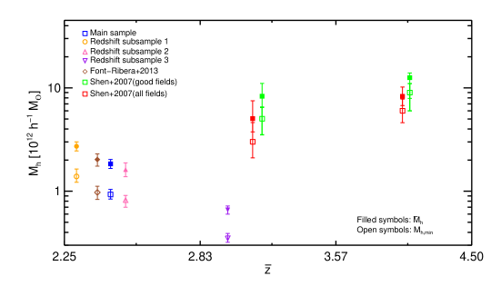
Figure 17: The evolution of minimum and characteristic halo mass [defined respectively by $b_{Q}=b(M>{M_{h,\rm min}})$ and $b_{Q}=b({\bar{M}_{h}})$] for the main sample and three redshift subsamples (detailed in Table 4) using the halo mass function from Tinker et al. (2010). We also measure these quantities for Shen et al. (2007) and Font-Ribera et al. (2013) based on their reported bias values. See Table 7 for the values and their 1-sigma uncertainties. The ”good fields” points have been offset slightly for visual clarity.

To compute the duty cycles in Table 7, we compare the cumulative luminosity function of quasars over a range of luminosities to the cumulative space density of halos over a range of host halo masses (Haiman & Hui, 2001; Martini & Weinberg, 2001):

$$f_{\rm duty}=\frac{\int_{L_{\rm min}}^{L_{\rm max}}\Phi(L)dL}{\int_{M_{\rm h,min}}^{\infty}\frac{dn}{dM}dM}.$$ (10)

We take the quasar luminosity function $\Phi(L)$ from Ross et al. (2013a), and report values of the number density based on this luminosity function in Table 7. Ross et al. (2013a) derive careful corrections to the number density of boss quasars by simulating quasars and attempting to reselect them with the boss targeting algorithm. This work on the boss selection function implies that boss only recovers $\sim 65$% of $z\sim 2.5$ quasars at $i\sim 20$ falling to only $\sim 35\%$ of $z\sim 2.5$ quasars at $i\sim 21$. (see Table 4 of Ross et al., 2013a). This selection function is reflected in the differences in our characteristic number densities in Table 6 and the number densities derived from $\Phi(L)$ in Table 7. In concert, the values from these two tables imply that our highest luminosity clustering sample is only $\sim 55\%$ complete and that our lowest luminosity clustering sample is only $\sim 30\%$ complete, in good agreement with Ross et al. (2013a).

Note that it is reasonable to integrate our halo masses to ${M_{h,\rm max}}=\infty$ in Eqn. 10, rather than to some other threshold value of ${M_{h,\rm max}}$. This is because, in the formalism of Eqn.  10, we are making no strong assumption that quasar clustering correlates strongly with quasar luminosity. In effect, we are assuming that quasars of a specific luminosity could occupy a broad range of halo masses. We relax this assumption later in this section by inverting our argument in order to predict the biases that would arise if halo mass was a tight, monotonic function of luminosity. In Table 7 we show our results for $f_{\rm duty}$, derived from Eqn. 10, for our main sample and for each of our redshift- and luminosity-based subsamples. Given the nearly constant values of ${M_{h,\rm min}}$ we derive from clustering, one can interpret the $f_{\rm duty}$ values as the probability that a halo above $M_{h}\approx 10^{12}\,h^{-1}M_{\odot}$ hosts a quasar in the corresponding luminosity range, and these probabilities are approximately proportional to the space densities of each subsample.

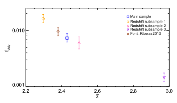
Figure 18: The evolution of the duty cycle for the main sample and three redshift subsamples (detailed in Table 4) using the halo mass function from Tinker et al. (2010) and the quasar luminosity function from Ross et al. (2013a). We also measure $f_{\rm duty}$ for Font-Ribera et al. (2013). See Table 7 for the $f_{\rm duty}$ values and their 1$\sigma$ uncertainties.

We derive error bars on $f_{\rm duty}$ by matching the $\pm 1\sigma$ values of ${M_{h,\rm min}}$ inferred from the $b_{Q}$ uncertainties. Figure 18 plots our derived values of $f_{\rm duty}$ against redshift for our primary sample and for our samples binned by redshift. We do not plot $z<2$ values because the implicit assumption of a monotonic relation between luminosity and halo mass is likely to become inaccurate at redshifts below $z\approx 2$ where the quasar luminosity function begins to decline. Our bias measurements imply a duty cycle of approximately 0.7% for our full sample, with a lower value of 0.1–0.2% for our highest redshift subsample. Disentangling whether this result is driven by redshift or luminosity is difficult. By virtue of the magnitude-limited nature of boss our highest redshift subsample also contains moderately more luminous quasars. It is plausible that the most luminous quasars should have smaller duty cycles. Our results are reasonably consistent with Fig. 14 of White et al. (2012), which suggests that duty cycle is only weakly dependent on luminosity at the level of 0.1–1%. However, we caution that the translation from quasar bias to duty cycle relies on the assumption that the sharp threshold in quasar luminosity corresponds to a sharp threshold in halo mass.

We can again compare our results to those of Shen et al. (2007), which imply higher duty cycles of $\sim 10$% at $z=3$ (White, Martini & Cohn, 2008; Shankar et al., 2010). White, Martini & Cohn (2008) quote $b_{Q}\sim 7$ or $b_{Q}\sim 8$ for the Shen et al. (2007) results using ‘all’ data or just the ‘best’ data. In our formalism, taking the Shen et al. (2007) value of $\Phi=5.592\times 10^{-7}\,(h^{-1}\rm Mpc)^{-3}$ at $z\sim 3$ (their Table 6) and adopting our mass function (Tinker et al., 2008) and cosmology, we derive $f_{\rm duty}\sim 2$% for $b_{Q}\sim 7$ and $f_{\rm duty}\sim 6$% for $b_{Q}\sim 8$. The factor of 3 difference in these duty cycles is driven by the steep relationship between bias and mass as halos become increasingly rare in the Tinker et al. (2010) model. In contrast, we measure $f_{\rm duty}\sim 0.2$% at $z\sim 3$ for our sample.

The broad reason for this order-of-magnitude difference is that Shen et al. (2007) measure far stronger clustering than we measure, implying that their quasar sample is far more biased than our sample. Their higher bias implies that their quasar sample occupies more massive and therefore far rarer halos than our sample. Although their quasars are brighter, and so less numerous than our quasars by a factor of 7, their measured bias implies that their quasars are in halos that are a factor of $\sim 70$ rarer than our halos (for their $b_{Q}\sim 7$ result). In other words, the lower density of the brighter Shen et al. (2007) quasar sample compared to our own does not compensate for the far lower density of the occupied halos implied by the Shen et al. (2007) measured bias. Taken at face value, the combination of our results with Shen et al. (2007) implies a sharp drop in the quasar duty cycle near $z\approx 3$. As we have previously noted in this section, other possible reasons for this discrepancy might include the difficulty in measuring quasar clustering for faint, high-redshift quasars, as well as uncertainties in the theoretical halo mass and bias function at high redshift (Tinker et al., 2010).

If quasar luminosity is a monotonic function of halo mass, then more luminous quasars should be more strongly clustered at a given redshift. As we have discussed previously in this section, this seems unlikely given our measurement that bias is not a strong function of luminosity. We can determine the biases that would be implied by a monotonic relationship between halo mass and luminosity by fixing $f_{\rm duty}$ in Eqn. 10. We can then assume that our brightest quasar sample occupies a mass range of ${M_{h,\rm min}}<M<\infty$, integrate over this range to determine ${M_{h,\rm min}}$ and then use this ${M_{h,\rm min}}$ as the maximum halo mass ${M_{h,\rm max}}$ for our next most luminous sample. In this manner, we can derive $M_{h}$ ranges for each of our luminosity subsamples and then integrate over those ranges (from ${M_{h,\rm min}}$ to ${M_{h,\rm max}}$ rather than always from ${M_{h,\rm min}}$ to $\infty$) in Eqn. 9 to derive bias values.

To begin, we assume that the host halos for each of our luminosity subsamples at $z=2.4$ have the value of $f_{\rm duty}=0.0073$ that we derived for the full sample at this redshift. For our highest luminosity bin, we then solve for the value of ${M_{h,\rm min}}$ from Eqn. 10 setting ${L_{\rm min}}=2.99\times 10^{46}\,{\rm erg\,s^{-1}}$ (see Table  7) and $f_{\rm duty}=0.0073$, obtaining ${M_{h,\rm min}}=2.39\times 10^{12}h^{-1}M_{\odot}$. For the next bin, we use Eqn. 10 with $f_{\rm duty}=0.0073$ and ${L_{\rm min}}=1.39\times 10^{46}\,{\rm erg\,s^{-1}}$, but now we set the upper limits of the integrals to the lower limits ${L_{\rm min}}$ and ${M_{h,\rm min}}$ for the higher luminosity bin, deriving a halo mass range ${M_{\rm h}}/10^{12}h^{-1}M_{\odot}=1.39$–2.39 for this luminosity bin. We repeat the process for the lowest luminosity bin, with ${L_{\rm max}}$ and ${M_{h,\rm max}}$ equal to the minimum values for the middle luminosity bin, deriving a halo mass range ${M_{\rm h}}/10^{12}h^{-1}M_{\odot}=0.99$–1.39.

These calculations of ${M_{h,\rm min}}$, where we impose a duty cycle and strictly require that more luminous quasars reside in higher mass halos, are conceptually different from those reported in Table 7, where we derived ${M_{h,\rm min}}$ for each luminosity sample independently based on its measured clustering bias. Here we are deriving ${M_{h,\rm min}}$ and ${M_{h,\rm max}}$ from the luminosity function, having chosen a duty cycle that will lead to the correct average bias across the full sample. Having derived ${M_{h,\rm min}}$ and ${M_{h,\rm max}}$ we then compute the predicted bias for each of our subsamples binned by luminosity using Eqn. 9.

We show the three predicted bias values as connected points in the right-hand panel of Fig. 16. Previous quasar clustering measurements at lower redshifts have shown little or no trend with luminosity (e.g., Shen et al. 2009; Padmanabhan et al. 2009). Shankar, Weinberg & Shen (2010) found that these results required a tight relation between luminosity and mass for low values of the duty cycle $(\sim 0.0001)$ but quite considerable scatter in the mass-luminosity relation for higher values of the duty cycle $(\sim 0.001)$. In essence, the meaning of the duty cycle itself therefore becomes complex in the presence of substantial luminosity scatter (see also Shankar, Weinberg & Miralda-Escudé (2013)). Further, we should be cautious about the exact value of $f_{\rm duty}$ inferred for our full sample, which is used to derive the results in Fig. 16, because it is likely that some lower mass halos host some of the quasars in our sample. We must therefore be careful not to strictly interpret our results in Fig. 16 as completely excluding a monotonic relationship between bias and luminosity. With these caveats in mind, however, the high value of $b_{Q}$ we have measured for quasar clustering near $z\sim 2.5$ implies that we are on a steeply rising portion of the $b(M_{h})$ relation, and the small statistical errors in Fig. 16 suggest a near-constant value for $b(L)$ and a correspondingly constant ${M_{h,\rm min}}(L)$. Taken at face value, then, our results imply that all halos above $M_{h}\approx 10^{12}\,h^{-1}M_{\odot}$ are able to host a quasar anywhere in our sample luminosity range, with little correlation between luminosity and halo mass.

A number of more sophisticated approaches to quasar clustering are possible, including abundance matching to galaxies (Conroy & White, 2013), halo occupation distribution (HOD) modeling (e.g. Degraf et al., 2011b), light curve models (Lidz et al., 2006), models that add scatter to the luminosity-halo mass relation (Shankar, Weinberg & Shen, 2010), and detailed evolutionary models that track black hole growth and model their relation to halos (e.g. Shankar et al., 2010). We refer the reader to White et al. (2012) for a more in-depth discussion of some of these issues. The quasar bias factor, while a single number, provides a critical quantitative constraint for any of these models. We have now measured this constraint with high precision at several luminosity thresholds over the redshift range $2.2\leq z\leq 3.4$.

$\Delta z$	$\Delta L$	$\Phi(L_{\rm min}<L<L_{\rm max})$	${M_{h,\rm min}}$	$\bar{M}_{\rm h}$	$f_{\rm duty}$
	($10^{46}\,{\rm erg\,s^{-1}}$)	$(10^{-6}\,h^{-1}\rm Mpc)^{-3}$	($10^{12}\,h^{-1}M_{\odot}$)	($10^{12}\,h^{-1}M_{\odot}$)
$2.20\leq z\leq 2.80$	$0.32\leq L\leq 31.33$	$7.709^{+0.999}_{-1.109}$	$0.93^{+0.11}_{-0.09}$	$1.84^{+0.19}_{-0.18}$	$0.00734^{+0.0014}_{-0.0011}$
$2.20\leq z<2.38$	$0.38\leq L\leq 30.20$	$11.641^{+1.881}_{-1.806}$	$1.39^{+0.16}_{-0.15}$	$2.72^{+0.28}_{-0.27}$	$0.0162^{+0.0031}_{-0.0025}$
$2.38\leq z<2.64$	$0.44\leq L\leq 31.33$	$7.804^{+1.693}_{-1.488}$	$0.82^{+0.15}_{-0.14}$	$1.62^{+0.26}_{-0.24}$	$0.0061^{+0.0016}_{-0.0014}$
$2.64\leq z\leq 3.40$	$0.57\leq L\leq 52.97$	$3.992^{+0.327}_{-0.565}$	$0.35^{+0.04}_{-0.07}$	$0.66^{+0.06}_{-0.06}$	$0.00145^{+0.0003}_{-0.0002}$
$2.20\leq z\leq 2.80$	$2.99\leq L\leq 31.33$	$1.846^{+0.137}_{-0.273}$	$1.03^{+0.12}_{-0.10}$	$2.02^{+0.20}_{-0.19}$	$0.0019^{+0.0004}_{-0.0003}$
$2.20\leq z\leq 2.80$	$1.39\leq L<2.99$	$2.635^{+0.182}_{-0.468}$	$0.92^{+0.12}_{-0.16}$	$1.87^{+0.27}_{-0.24}$	$0.0023^{+0.0006}_{-0.0004}$
$2.20\leq z\leq 2.80$	$0.32\leq L<1.39$	$3.228^{+0.955}_{-0.369}$	$1.26^{+0.26}_{-0.15}$	$2.46^{+0.45}_{-0.40}$	$0.0044^{+0.0015}_{-0.0008}$

Table 7: The first three columns are the characteristics of each subsample; the redshift range, the luminosity range and the number density of quasars calculated using the luminosity function of Ross et al. (2013a). The 4th and 5th columns are the minimum and the characteristic halo mass based on the halo mass function (Tinker et al., 2008) and bias model (Tinker et al., 2010) at the average redshift of the sample (see Eqn. 9). The 6th column lists the duty cycle for the quasars in each sample, which is derived from ${M_{h,\rm min}}$ and $\Phi$ (see Eqn. 10). $f_{\rm duty}$ is expressed as a fraction of the Hubble time (9.785 $h^{-1}\,{\rm Gyrs}$).

7 Conclusions

We measured the real and redshift-space correlation functions for a uniformly selected sample of 55,826 ngc-core quasars from the final data release of sdss-iii/boss over the redshift range $2.2\leq z\leq 2.8$. We also investigated the luminosity dependence of quasar clustering by splitting this ngc-core sample into three bins of absolute magnitude containing approximately equal numbers of quasars. We do not detect a significant luminosity dependence to clustering strength for boss quasars over a factor $\approx 10$ range in luminosity. Our clustering results are summarized in Table 5.

This work provides precise quasar clustering measurements near $z\sim 2.5$, using samples of tens-of-thousands of quasars. We more than double the sample size compared to the earlier boss work of White et al. (2012), and extend measurements of the real-space projected 2PCF to larger scales. Our best-fit correlation lengths and slopes are in good agreement with, but more accurate and more precise than, those of White et al. (2012).

In order to investigate the redshift dependence of quasar clustering, we extended the upper redshift limit of our boss sample to $z=3.4$ and divided the resulting set of 73,884 quasars into three redshift subsamples of roughly equal size. Our fitting results for the three redshift subsamples (see Table 5), suggest that the correlation length does not evolve strongly over the redshift range $2.2\leq z\leq 3.4$. When compared with earlier work (see Fig. 12), this result suggests that $r_{0}$ evolves by no more than a factor $\sim 2$ from $z\sim 3$ to $z\sim 1$. We fit our redshift-space correlation functions to a power spectrum for dark matter halos from halofit (Smith et al., 2003) modified by the correction for redshift space distortions from Kaiser (1987). The bias of our quasars does not depend strongly on either redshift or luminosity within our sample and is roughly $b_{Q}\sim 3.5$ at $z\sim 2.5$.

We adopted the halo bias model of Tinker et al. (2010) in order to use our measured biases to estimate the average halo masses of quasars in our main (ngc-core) sample and in our three redshift subsamples (see Table 7). The estimated characteristic dark matter halo mass that we derived for quasars over the redshift range $2.2\leq z\leq 3.4$ covers a relatively wide range of halo masses from $\sim 0.6$ to $3\times 10^{12}\,h^{-1}\rm M_{\odot}$ because a higher mass is required to yield the same bias at a lower redshift. By integrating our adopted bias model over the halo mass function of Tinker et al. (2008) we determined the minimum halo mass corresponding to our measured biases, deriving ${M_{h,\rm min}}$ values from $\sim 0.3$ to $1.5\times 10^{12}\,h^{-1}\rm M_{\odot}$.

By comparing the number density of halos above this mass threshold from Tinker et al. (2008) to the quasar luminosity function for boss from Ross et al. (2013a) we found that the duty cycles for our main and redshift subsamples are $f_{\rm duty}\sim 1$%, with our highest redshift (and therefore most luminous) subsample approaching $f_{\rm duty}\sim 0.2$%. These values of $f_{\rm duty}\sim 1$% are in agreement with previous works, and are broadly consistent with quasars being short-lived and episodic (as argued by, e.g., Croom et al., 2005) but are also not inconsistent with a mixed population of quasars—consisting of a bursty population igniting as their parent halos grow, combined with a larger fraction of shorter-lived quasars (see, e.g., the discussion in White et al., 2012). These values of $f_{\rm duty}$ implicitly assume that halos with mass below ${M_{h,\rm min}}$ do not host quasars in our sample, and they then describe the probability that a randomly selected halo above ${M_{h,\rm min}}$ is active above our sample luminosity threshold at any given time.

There are two somewhat surprising results in our analysis. The first is a nearly constant strength of clustering with luminosity. We investigated a model in which the quasar luminosity is a monotonic function of host halo mass, using the Ross et al. (2013b) luminosity function to infer halo mass ranges from quasar space densities assuming the duty cycle ($f_{\rm duty}\sim 0.7\%$) derived from fitting the full sample. This model predicts a quasar bias that rises from $b_{Q}\sim 3.1$ for our faintest sample to $b_{Q}\sim 4.5$ for our brightest sample, clearly inconsistent with our measurements. We conclude that there must be substantial scatter between halo mass and quasar luminosity in this redshift/luminosity range. A broad short-timescale scatter in Eddington ratio has been proposed both from observational and theoretical standpoints in previous studies (e.g., Hopkins & Hernquist, 2009; Kauffmann & Heckman, 2009; Novak, Ostriker & Ciotti, 2011; Aird et al., 2012; Bongiorno et al., 2012; Gabor & Bournaud, 2013; Hickox et al., 2014; Veale, White & Conroy, 2014; Schawinski et al., 2015), which further argues against a tight, monotonic relationship between luminosity and mass. Our conclusion is stronger than that reached from previous studies at lower redshift because of our high statistical precision and because the high bias of our quasars puts us on the steeply rising portion of the $b(M_{h})$ relation.

The second surprise is the difference between our measured host halo masses and duty cycles when compared to the work of Shen et al. (2007). At $z\sim 3$ we derive halo masses and duty cycles that are close to an order-of-magnitude smaller than those of Shen et al. (2007). Both of these results are driven by Shen et al. (2007) measuring that quasars cluster far more strongly than we have found in this work. The high biases found by Shen et al. (2007) imply that the quasars they use are in far rarer halos than those we study, by a factor of $\sim 70\times$. The quasars studied by Shen et al. (2007) are brighter than the boss sample we study, and so they are also rarer, but only by a factor of $\sim 7\times$. The fact that the Shen et al. (2007) quasar sample has a number density nearly $10\times$ lower than our boss sample but an implied halo abundance nearly $100\times$ lower is the main discrepancy between this earlier work and our own results. A strong dependence of quasar clustering on luminosity or redshift could explain the difference of results, but no hints of such dependence are seen within our sample.

Perhaps the most likely explanation of these differences lies in the difficulty of studying clustering of high redshift quasars targeted near the limits of an imaging survey. This is particularly true near $z\sim 3$, where quasar colours resemble those of stars. Our analysis takes advantage of improvements in SDSS photometric calibration and target selection algorithms as well as much larger numbers that afford greater measurement precision. The excellent agreement between our measured quasar bias and the value found by Font-Ribera et al. (2013) from cross-correlation with the Lyman-$\alpha$ forest is strong evidence that our full sample result, at least, is not affected by variations in target selection efficiency or redshift completeness (which would both affect auto-correlations but not cross-correlations). Nonetheless, the difference from earlier results at $z>3$ highlights the importance of studying large quasar samples selected from deep imaging with well controlled systematics.

This paper reports measurements of quasar clustering using the final sample from the sdss-iii/boss survey. The prospects for further refining measurements of quasar clustering across a range of redshifts are excellent. The sdss-iv/eboss survey has just begun (see Myers et al. 2015) and will ultimately result in a uniformly selected sample of $\sim$500,000 quasars over a range of redshift from $z\sim 0.7$ to $z\sim 3.5$. sdss-iv/eboss should more than double the number of uniformly selected quasars at moderate redshift ($2.2<z<3.5$) compared to the sample used in this paper, and it will provide an opportunity to measure quasar clustering across most of cosmic history in a single, consistently selected sample.

Appendix A The “BOSSQSOMASK” software

In order to make clustering measurements it is necessary to create a random catalog that mimics the selection function of the data but that is otherwise unclustered (see $\S$2). Here we introduce the “bossqsomask” package—a series of reasonably mature IDL codes that can be used to produce random catalogs that mimic the boss core quasar selection. bossqsomask has been used in previous papers (e.g., White et al., 2012; Karagiannis, Shanks & Ross, 2014) but we make the current version available online with the publication of this paper. Each bossqsomask routine has a header documenting its purpose, but here we highlight the critical steps needed to produce coordinates and redshifts for random objects according to the angular spectroscopic completeness and redshift distribution of boss quasars.

To mimic the selection of boss quasars, approximately 300,000 distinct spherical caps are created using the mangle software (Swanson et al., 2008). To cull areas of the survey that greatly affect the quasar density, we use veto masks developed to analyze boss galaxy clustering (see, e.g., White et al., 2011; Anderson et al., 2012; Ross et al., 2012a). The angular completeness of the survey is tracked in regions defined by a unique set of overlapping spectroscopic tiles (called a sector; see Blanton et al., 2003). The angular completeness in each sector (called $f_{\rm comp}$ in this paper) is defined to be the ratio of the number of quasars for which good spectra are obtained to the number of all targets in the target list. The bossqsomask code takes the minimum acceptable angular completeness as an input (e.g., $f_{\rm comp}$=0.75 can be sent to indicate that the survey should be limited to areas with angular completeness greater than 75%, as was used in this paper).

In the rest of this appendix, we detail the specific requirements and procedures for the bossqsomask software. There are numerous observational effects that have a second-order effect on target density in boss (e.g., Ross et al., 2012a). Such effects are particularly prevalent in the sgc region of boss (see the eboss target selection papers, Myers et al., Prakash et al. 2015). bossqsomask does not attempt to correct for these higher-order effects, and so users should not trust the software to account for subtle differences in target density between the random catalog and the quasar sample—differences that can cause deviations from zero clustering amplitude on very large scales.

A.1 File and system requirements

bossqsomask requires a list of all objects that would have been targeted as a boss core quasar, i.e., all point sources in the boss area that have an xdqso probability above 0.424 to the magnitude limit of boss. An appropriate file is included in the bossqsomask data directory, and is used to make the psuedo-core of all quasars that “should have been targeted” (i.e. if angular completeness was 100%).

The package requires two environment variables to be defined: $BOSSQSOMASK_DIR and $BOSSLSS_DIR. These variables are necessary so that bossqsomask can find masks as well as code functions. $BOSSLSS_DIR must contain all of the masking files listed as part of the galaxy clustering package at, e.g., http://www.sdss3.org/dr9/tutorials/lss_galaxy.php. A working copy of the idlutils software suite is needed, and the binaries have to be properly compiled such that, e.g., mangle’s ransack procedure in $IDLUTILS_DIR/src is functional. Running the sequence of the following codes will produce a random catalog (with the user’s desired size and completeness level) using the survey masks and list of core targets.

A.2 Main steps

1) Making the xd core target list (make_xd_core.pro):

This code takes the file of all xdqso core targets as an input and constructs the pseudo-core target list (called data/xdcore/xdcore.fits). The code uses veto masks for bright stars, center posts, bad $u$-columns and bad-photometry fields (many of these masks reside in the directory pointed to by $BOSSLSS_DIR).

2) Making the xd spAll file (make_xdspall.pro):

This step requires the latest version of the boss spAll file that contains the spectroscopic information for boss targets (e.g. spAll-v5_7_0). The spAll file can be downloaded by running pro/get/get_spall.pro, which limits the spAll file to just the relevant information (the “mini-spAll” file) and places it in the directory data/spall.

Once the mini-spAll file is in the correct path, make_xdspall.pro cross-matches observed objects in the spAll file with targets from the xdcore.fits file (produced in the first step), and makes a file of matched targets and spectra called data/compfiles/xdspall.fits.

3) Assigning weights to the sectors of the survey mask (make_sector_completeness.pro):

In order to construct the random catalog with the correct angular density and to select only sectors at the user-specified completeness level requires a weight that tracks the angular completeness for quasars in each sector of boss. This code takes the files of targets and spectra, obtains the boss sector geometry from the $BOSSLSS_DIR and calculates the angular completeness in each sector.

Several local files are written that are more manageable than the comprehensive target files. Most notably the file data/compfiles/xdspallmask.fits, which indicates which sector of the mask each target occupies. In addition, smaller mangle polygon files are written that contain the subset of sectors that are relevant to boss quasars (data/compfiles/bosspoly.fits and data/compfiles/bosspoly.ply).

4) Constructing the angular distribution of objects in the random catalog (make_angular_random_catalog.pro):

This code reads the file of which sectors are relevant for boss quasars (e.g., bosspoly.ply) as well as the file that indicates the mask sector and weight for each target (xdspall.fits) and creates files of targets and spectroscopically confirmed targets based on the user-specified completeness (denoted completeness), called xd_compcompleteness.fits and xdspall_compcompleteness.fits.

The code also determines the sectors that have a higher weight than the user-specified completeness level, and then angularly populates those sectors (according to their weight) with $N$ times more total random points than boss quasar targets using mangle’s ransack procedure. $N$ is specified as an input by the user.

5) Assigning redshifts to objects in the random catalog (make_redshift_random_catalog.pro):

Based on spectroscopically-confirmed quasars in the sectors derived by make_angular_random_catalog.pro this code generates a random redshift from the cumulative distribution of quasar redshifts. The code outputs final data and random catalogs in fits format of the size and at the completeness level specified by the user. As with all files generated during the construction of the random catalog, the final output files are stored in the directory data/compfiles. The files are called data_compcompleteness.fits and randoms_compcompleteness.fits where completeness is the user-specified completeness.

A.3 Examining the produced random catalog

Finally, the procedure diagnostics.pro is provided to help diagnose whether bossqsomask is functioning as expected. diagnostics.pro can conduct four different tests:

1. Angular distribution test: the angular distribution of data and random objects should match

2. Redshift distribution test: the redshift distribution of data and random objects should match

3. Weights versus number of random points test: the number of random points in each sector should be proportional to “completeness$\times$area” for each sector at the user-specified completeness level

4. Weights versus number of objects test: the number of data points in each sector should roughly be proportional to “completeness$\times$area” for each sector at the user-specified completeness level

References

- Agarwal et al. (2014) Agarwal N. et al., 2014, JCAP, 4, 7
- Aihara et al. (2011) Aihara H. et al., 2011, \apjs, 193, 29
- Aird et al. (2012) Aird J. et al., 2012, \apj, 746, 90
- Alexander & Hickox (2012) Alexander D. M., Hickox R. C., 2012, \apjs, 56, 93
- Allevato et al. (2011) Allevato V. et al., 2011, \apj, 736, 99
- Allevato et al. (2014) Allevato V. et al., 2014, \apj, 796, 4
- Anderson et al. (2014) Anderson L. et al., 2014, \mnras, 441, 24
- Anderson et al. (2012) Anderson L. et al., 2012, \mnras, 427, 3435
- Aubourg et al. (2014) Aubourg É. et al., 2014, ArXiv e-prints
- Behroozi, Conroy & Wechsler (2010) Behroozi P. S., Conroy C., Wechsler R. H., 2010, \apj, 717, 379
- Benson et al. (2000) Benson A. J., Cole S., Frenk C. S., Baugh C. M., Lacey C. G., 2000, \mnras, 311, 793
- Berlind & Weinberg (2002) Berlind A. A., Weinberg D. H., 2002, \apj, 575, 587
- Béthermin et al. (2012) Béthermin M. et al., 2012, \apjl, 757, L23
- Blanton et al. (2003) Blanton M. R., Lin H., Lupton R. H., Maley F. M., Young N., Zehavi I., Loveday J., 2003, \aj, 125, 2276
- Bolton et al. (2012) Bolton A. S. et al., 2012, \aj, 144, 144
- Bongiorno et al. (2012) Bongiorno A. et al., 2012, \mnras, 427, 3103
- Bovy et al. (2011) Bovy J. et al., 2011, \apj, 729, 141
- Budavári et al. (2001) Budavári T. et al., 2001, \aj, 122, 1163
- Caplar, Lilly & Trakhtenbrot (2014) Caplar N., Lilly S., Trakhtenbrot B., 2014, ArXiv e-prints
- Chatterjee et al. (2012) Chatterjee S., Degraf C., Richardson J., Zheng Z., Nagai D., Di Matteo T., 2012, \mnras, 419, 2657
- Cole & Kaiser (1989) Cole S., Kaiser N., 1989, \mnras, 237, 1127
- Conroy & White (2013) Conroy C., White M., 2013, \apj, 762, 70
- Cooray & Sheth (2002) Cooray A., Sheth R., 2002, \physrep, 372, 1
- Croom et al. (2005) Croom S. M. et al., 2005, \mnras, 356, 415
- Croom et al. (2004) Croom S. M., Smith R. J., Boyle B. J., Shanks T., Miller L., Outram P. J., Loaring N. S., 2004, \mnras, 349, 1397
- Croton et al. (2006) Croton D. J. et al., 2006, \mnras, 365, 11
- da Ângela et al. (2005) da Ângela J., Outram P. J., Shanks T., Boyle B. J., Croom S. M., Loaring N. S., Miller L., Smith R. J., 2005, \mnras, 360, 1040
- da Ângela et al. (2008) da Ângela J. et al., 2008, \mnras, 383, 565
- Davis & Peebles (1983) Davis M., Peebles P. J. E., 1983, \apj, 267, 465
- Dawson et al. (2013) Dawson K. S. et al., 2013, \aj, 145, 10
- DeGraf et al. (2012) DeGraf C., Di Matteo T., Khandai N., Croft R., Lopez J., Springel V., 2012, \mnras, 424, 1892
- Degraf et al. (2011a) Degraf C., Oborski M., Di Matteo T., Chatterjee S., Nagai D., Richardson J., Zheng Z., 2011a, \mnras, 416, 1591
- Degraf et al. (2011b) Degraf C., Oborski M., Di Matteo T., Chatterjee S., Nagai D., Richardson J., Zheng Z., 2011b, \mnras, 416, 1591
- Di Matteo et al. (2012) Di Matteo T., Khandai N., DeGraf C., Feng Y., Croft R. A. C., Lopez J., Springel V., 2012, \apjl, 745, L29
- DiPompeo et al. (2014a) DiPompeo M. A., Myers A. D., Hickox R. C., Geach J. E., Hainline K. N., 2014a, \mnras, 442, 3443
- DiPompeo et al. (2014b) DiPompeo M. A., Myers A. D., Hickox R. C., Geach J. E., Holder G., Hainline K. N., Hall S. W., 2014b, ArXiv e-prints
- Donoso et al. (2014) Donoso E., Yan L., Stern D., Assef R. J., 2014, \apj, 789, 44
- Eisenstein et al. (2011) Eisenstein D. J. et al., 2011, \aj, 142, 72
- Fan et al. (1999) Fan X. et al., 1999, \apjl, 526, L57
- Ferrarese (2002) Ferrarese L., 2002, \apj, 578, 90
- Ferrarese & Merritt (2000) Ferrarese L., Merritt D., 2000, \apjl, 539, L9
- Font-Ribera et al. (2013) Font-Ribera A. et al., 2013, JCAP, 5, 18
- Fukugita et al. (1996) Fukugita M., Ichikawa T., Gunn J. E., Doi M., Shimasaku K., Schneider D. P., 1996, \aj, 111, 1748
- Gabor & Bournaud (2013) Gabor J. M., Bournaud F., 2013, \mnras, 434, 606
- Gebhardt et al. (2000) Gebhardt K. et al., 2000, \apjl, 539, L13
- Górski et al. (2005) Górski K. M., Hivon E., Banday A. J., Wandelt B. D., Hansen F. K., Reinecke M., Bartelmann M., 2005, \apj, 622, 759
- Gunn et al. (1998) Gunn J. E. et al., 1998, \aj, 116, 3040
- Gunn et al. (2006) Gunn J. E., Siegmund W. A., Mannery E. J., Owen R. E., Hull a. . c.-a., 2006, \aj, 131, 2332
- Haiman & Hui (2001) Haiman Z., Hui L., 2001, \apj, 547, 27
- Hennawi et al. (2006) Hennawi J. F. et al., 2006, \aj, 131, 1
- Hickox et al. (2009) Hickox R. C. et al., 2009, \apj, 696, 891
- Hickox et al. (2014) Hickox R. C., Mullaney J. R., Alexander D. M., Chen C.-T. J., Civano F. M., Goulding A. D., Hainline K. N., 2014, \apj, 782, 9
- Hickox et al. (2011) Hickox R. C. et al., 2011, \apj, 731, 117
- Hinshaw et al. (2013) Hinshaw G. et al., 2013, \apjs, 208, 19
- Ho et al. (2015) Ho S. et al., 2015, JCAP, 5, 40
- Hopkins & Hernquist (2009) Hopkins P. F., Hernquist L., 2009, \apj, 698, 1550
- Hopkins et al. (2007) Hopkins P. F., Lidz A., Hernquist L., Coil A. L., Myers A. D., Cox T. J., Spergel D. N., 2007, \apj, 662, 110
- Kaiser (1984) Kaiser N., 1984, \apjl, 284, L9
- Kaiser (1987) Kaiser N., 1987, \mnras, 227, 1
- Karagiannis, Shanks & Ross (2014) Karagiannis D., Shanks T., Ross N. P., 2014, \mnras, 441, 486
- Kauffmann & Heckman (2009) Kauffmann G., Heckman T. M., 2009, \mnras, 397, 135
- Kirkpatrick et al. (2011) Kirkpatrick J. A., Schlegel D. J., Ross N. P., Myers A. D., Hennawi J. F., Sheldon E. S., Schneider D. P., Weaver B. A., 2011, \apj, 743, 125
- Kormendy & Ho (2013) Kormendy J., Ho L. C., 2013, \araa, 51, 511
- Kormendy & Richstone (1995) Kormendy J., Richstone D., 1995, \araa, 33, 581
- Krumpe et al. (2012) Krumpe M., Miyaji T., Coil A. L., Aceves H., 2012, \apj, 746, 1
- Landy & Szalay (1993) Landy S. D., Szalay A. S., 1993, \apj, 412, 64
- Lidz et al. (2006) Lidz A., Hopkins P. F., Cox T. J., Hernquist L., Robertson B., 2006, \apj, 641, 41
- Magorrian et al. (1998) Magorrian J. et al., 1998, \aj, 115, 2285
- Martini & Weinberg (2001) Martini P., Weinberg D. H., 2001, \apj, 547, 12
- Moster et al. (2010) Moster B. P., Somerville R. S., Maulbetsch C., van den Bosch F. C., Macciò A. V., Naab T., Oser L., 2010, \apj, 710, 903
- Mullaney et al. (2012) Mullaney J. R. et al., 2012, \mnras, 419, 95
- Myers et al. (2007a) Myers A. D., Brunner R. J., Nichol R. C., Richards G. T., Schneider D. P., Bahcall N. A., 2007a, \apj, 658, 85
- Myers et al. (2007b) Myers A. D., Brunner R. J., Richards G. T., Nichol R. C., Schneider D. P., Bahcall N. A., 2007b, \apj, 658, 99
- Myers et al. (2006) Myers A. D. et al., 2006, \apj, 638, 622
- Myers et al. (2005) Myers A. D., Outram P. J., Shanks T., Boyle B. J., Croom S. M., Loaring N. S., Miller L., Smith R. J., 2005, \mnras, 359, 741
- Myers et al. (2008) Myers A. D., Richards G. T., Brunner R. J., Schneider D. P., Strand N. E., Hall P. B., Blomquist J. A., York D. G., 2008, \apj, 678, 635
- Nandra et al. (2007) Nandra K. et al., 2007, \apjl, 660, L11
- Novak, Ostriker & Ciotti (2011) Novak G. S., Ostriker J. P., Ciotti L., 2011, \apj, 737, 26
- Oke & Gunn (1983) Oke J. B., Gunn J. E., 1983, \apj, 266, 713
- Padmanabhan et al. (2009) Padmanabhan N., White M., Norberg P., Porciani C., 2009, \mnras, 397, 1862
- Peacock & Smith (2000) Peacock J. A., Smith R. E., 2000, \mnras, 318, 1144
- Peebles (1980) Peebles P. J. E., 1980, in Annals of the New York Academy of Sciences, Vol. 336, Ninth Texas Symposium on Relativistic Astrophysics, Ehlers J., Perry J. J., Walker M., eds., pp. 161–171
- Planck Collaboration et al. (2014) Planck Collaboration et al., 2014, \aap, 571, A16
- Porciani, Magliocchetti & Norberg (2004) Porciani C., Magliocchetti M., Norberg P., 2004, \mnras, 355, 1010
- Porciani & Norberg (2006) Porciani C., Norberg P., 2006, \mnras, 371, 1824
- Reid et al. (2012) Reid B. A. et al., 2012, \mnras, 426, 2719
- Richards et al. (2002) Richards G. T. et al., 2002, \aj, 123, 2945
- Richards et al. (2001) Richards G. T. et al., 2001, \aj, 121, 2308
- Richards et al. (2006) Richards G. T. et al., 2006, \apjs, 166, 470
- Richards et al. (2009) Richards G. T. et al., 2009, \apjs, 180, 67
- Richardson et al. (2013) Richardson J., Chatterjee S., Zheng Z., Myers A. D., Hickox R., 2013, \apj, 774, 143
- Richardson et al. (2012) Richardson J., Zheng Z., Chatterjee S., Nagai D., Shen Y., 2012, \apj, 755, 30
- Ross et al. (2011) Ross A. J. et al., 2011, \mnras, 417, 1350
- Ross et al. (2012a) Ross A. J. et al., 2012a, \mnras, 424, 564
- Ross et al. (2013a) Ross N. P. et al., 2013a, \apj, 773, 14
- Ross et al. (2013b) Ross N. P. et al., 2013b, \apj, 773, 14
- Ross et al. (2012b) Ross N. P. et al., 2012b, \apjs, 199, 3
- Ross et al. (2009) Ross N. P. et al., 2009, \apj, 697, 1634
- Schawinski et al. (2015) Schawinski K., Koss M., Berney S., Sartori L., 2015, ArXiv e-prints
- Schneider et al. (2010) Schneider D. P. et al., 2010, \aj, 139, 2360
- Scoccimarro et al. (2001) Scoccimarro R., Sheth R. K., Hui L., Jain B., 2001, \apj, 546, 20
- Scranton et al. (2002) Scranton R. et al., 2002, \apj, 579, 48
- Seljak (2000) Seljak U., 2000, \mnras, 318, 203
- Shankar (2009) Shankar F., 2009, \apj, 53, 57
- Shankar et al. (2010) Shankar F., Crocce M., Miralda-Escudé J., Fosalba P., Weinberg D. H., 2010, \apj, 718, 231
- Shankar, Weinberg & Miralda-Escudé (2013) Shankar F., Weinberg D. H., Miralda-Escudé J., 2013, \mnras, 428, 421
- Shankar, Weinberg & Shen (2010) Shankar F., Weinberg D. H., Shen Y., 2010, \mnras, 406, 1959
- Shen et al. (2010) Shen Y. et al., 2010, \apj, 719, 1693
- Shen et al. (2007) Shen Y. et al., 2007, \aj, 133, 2222
- Shen et al. (2009) Shen Y. et al., 2009, \apj, 697, 1656
- Silverman et al. (2008) Silverman J. D. et al., 2008, \apj, 679, 118
- Smee et al. (2013) Smee S. A. et al., 2013, \aj, 146, 32
- Smith et al. (2003) Smith R. E. et al., 2003, \mnras, 341, 1311
- Swanson et al. (2008) Swanson M. E. C., Tegmark M., Blanton M., Zehavi I., 2008, \mnras, 385, 1635
- Tegmark et al. (2004) Tegmark M., Blanton M. R., Strauss M. A., Hoyle F., Schlegel D., SDSS Collaboration, 2004, \apj, 606, 702
- Tinker et al. (2008) Tinker J., Kravtsov A. V., Klypin A., Abazajian K., Warren M., Yepes G., Gottlöber S., Holz D. E., 2008, \apj, 688, 709
- Tinker et al. (2010) Tinker J. L., Robertson B. E., Kravtsov A. V., Klypin A., Warren M. S., Yepes G., Gottlöber S., 2010, \apj, 724, 878
- Veale, White & Conroy (2014) Veale M., White M., Conroy C., 2014, \mnras, 445, 1144
- Viero et al. (2014) Viero M. P. et al., 2014, \apjs, 210, 22
- Viero et al. (2013a) Viero M. P. et al., 2013a, \apj, 779, 32
- Viero et al. (2013b) Viero M. P. et al., 2013b, \apj, 772, 77
- Weinstein et al. (2004) Weinstein M. A. et al., 2004, \apjs, 155, 243
- White et al. (2011) White M. et al., 2011, \apj, 728, 126
- White, Hernquist & Springel (2001) White M., Hernquist L., Springel V., 2001, \apjl, 550, L129
- White, Martini & Cohn (2008) White M., Martini P., Cohn J. D., 2008, \mnras, 390, 1179
- White et al. (2012) White M. et al., 2012, \mnras, 424, 933
- Wyithe & Loeb (2005) Wyithe J. S. B., Loeb A., 2005, \apj, 621, 95
- Yèche et al. (2010) Yèche C. et al., 2010, \aap, 523, A14
- Zehavi et al. (2002) Zehavi I. et al., 2002, \apj, 571, 172
- Zehavi et al. (2011) Zehavi I. et al., 2011, \apj, 736, 59
- Zheng et al. (2005) Zheng Z. et al., 2005, \apj, 633, 791
- Zheng, Coil & Zehavi (2007) Zheng Z., Coil A. L., Zehavi I., 2007, \apj, 667, 760