A Lagrangian-Driven Cellular Automaton Supporting Quantum Field Theory

Abstract

Models of areas of physics in terms of cellular automata have become increasingly popular. Cellular automata (CAs) support the modeling of systems with discrete state component values and enforce the comprehensive specification of the dynamic evolution of such systems. Because many areas of physics can be described by starting with a specific Lagrangian, the idea to derive a cellular automaton directly from the Lagrangian (or similar construct, such as the Hamiltonian or action) is not new. Previous work, however, indicated that the classical CA may not be a sufficient basis for the modeling of more advanced physics theories, such as quantum field theory. Specifically, the modeling of interactions in quantum field theory requires extensions and modifications of the classical CA. This paper describes a proposal for an extended cellular automaton that is suited for support of quantum field theory.

Keywords: Cellular automaton, Lagrangian, Equation of motion, Quantum field theory

1 Introduction

Attempts to describe models of areas of physics in terms of cellular automata (CAs) reach back to E. Fredkin, 1990 [9], and S. Wolfram’s work in 2002 [22]. Some of these works applied cellular automata to areas of quantum theory (QT) (see [11], [6], [7], [13]). The relation of CAs to the Lagrangian or a related construct, such as the Hamiltonian or an action, has been addressed in [16], [6], [7].

Two items that make CAs especially attractive for the modeling of specific areas of physics are the following:

1. CAs imply discreteness of the variables that constitute the system state.
   Generally and traditionally, physics theories do not assume discrete state variables. The discrete eigenstates of quantum theory represent only a special case of discreteness. Discreteness with other special aspects is addressed in [13], [14] and [3].

2. CAs represent a functional model of the subject theory, i.e., a model that specifies the dynamical evolution of the system in terms of state transitions.

While these properties are desirable for special types of formulations of physics theories (e.g., [13], [14], [3]), they represent a challenge at the same time because existing standard formulations of areas of physics, in general, are well-suited neither for discreteness nor for functional descriptions.

After trying to formulate a Lagrangian-based and CA-based model of different areas of physics, it turned out that the classical CA is not a sufficient basis for the modeling of more advanced areas of physics (such as quantum field theory) and that the Lagrangian provides much but not the complete content of the physics theories. Thus, the objective of this paper is also the identification of missing pieces and deficiencies and the provision of proposals to overcome these deficiencies.

Section 2 contains a proposal for a CA called QFTCA, which is an extension of the classical CA. In section 3, for some major areas of classical physics (e.g., Newtonian mechanics, waves, fields, non-relativistic quantum mechanics), the Lagrangian is transformed into a CA-based functional model. Quantum field theory (QFT), the main subject of this paper, is addressed in sections 5 and 6. Section 6 describes a CA-based functional model for interactions in QFT. The CAs are, as much as possible, derived from the Lagrangian for the subject areas of physics. More precisely, the CAs are derived from the equations of motion that are derived from the Lagrangian. The transformation of the equation of motion into a CA, which shows the dynamical state evolution in accordance with the equation of motion, is relatively straightforward. However, the generation of a CA that provides a more complete functional model of the subject area of physics requires additional specifications that cannot be deduced solely from the equation of motion. Therefore, the CA-based functional model of QFT interactions (section 6) is based on the functional model of QFT interactions described in [3].

The CA described in this paper has been accompanied by a computer model QFTCA, which enables experimentation with alternative solutions and the generation of the illustrations of examples contained in this paper. However, the computer model is not the subject of the present paper. A rough overview of the computer model is given in appendix A.

2 The Cellular Automaton

2.1 The classical Cellular Automaton

The classical CA consists of a k-dimensional grid of cells. The state of the CA is given by the totality of the states of the individual cells.

state $=\{s_{1},...,s_{n}\}$
With traditional standard CAs, the cell states uniformly consist of the same state components

$s_{i}=\{s^{1}_{i},...,s^{j}_{i}\}$
Typically, the number of state components, j, is 1, and the possible values are restricted to integer numbers. The dynamical evolution of the CA is given by the ”update-function”, which computes the new state of a cell as a function of its current state and the states of the neighbor cells.

Standard-CellularAutomaton(initial-state)  :=     // transition function
state = initial-state;
DO FOREVER {
   state = update-function(state, timestep);
   IF ( termination-state(state))  STOP;
}

The full functionality and complexity of a particular cellular automaton is concentrated in the update-function. As Wolfram (see [22]) and others (see, for example, [15]) showed, a large variety of process types (e.g., stable, chaotic, pseudo-random, oscillating) can be achieved with relatively simple update-functions.

2.2 The extended Cellular Automaton, QFTCA

To enable support of the most advanced areas of physics (e.g., QT/QFT), including support of multiple fields and particles, a cellular automaton QFTCA is defined, which is an extension of the classical CA, made by embedding the CA into an overall physics-based system structure. The embedding into the physics-based system structure affects two aspects: the structure of the state of the system and the functions for the dynamic evolution of the system.

2.2.1 State structure

The states of QFTCA cannot be expressed solely by the collection of cell states. In addition to the ”local” information contained in the CA cells, non-local information about physical objects (e.g., waves, particles and fields) have to be part of the system state. Position related (i.e., local) information of physical objects can be assigned to cell states. Other (non-local) information has to be kept in addition to the cell states.

System-state :=
  CA-cells,
  Particle-set,
  Field-set;

The CA cells {$s_{1},...,s_{n}$ } represent the space. The particles and the fields have to be mapped to the space, i.e., to the CA cells. The state components of an individual cell depend on the particle or field to which the cell belongs. The set of state components is thus not uniform for all cells. The possible values of the state components are not restricted to integer values (however, a discrete value set may be assumed with specific types of state components). For the mapping of the overall system state to the CA cells, the following hold true:

• For the QFTCA described in this paper, it is left open which state components are assigned to CA cells as opposed to state components that are kept with the physical objects. It has to be ensured that the cells (i.e., space points) belonging to a physical object can be determined and vice versa; i.e., that the physical objects occupying a CA cell can be determined.

• A physical object may cover multiple cells.

• A cell may be covered by multiple physical objects.

• Time is not a (fourth) dimension of QFTCA. Instead, the time derivatives such as $\partial\psi/\partial t,dx/dt$ and $p^{\mu}$, are explicit parts of the system state.

The above-described state structure and timing considerations result in differing contents of CA cells and CA update-functions, which depend on the physical objects assigned to the cells.

2.2.2 Evolution of the system state

The structuring of the overall system state into the CA cells and the superimposed physical objects was also motivated by the differing update requirements of the physical objects.

QFTCA (initial-state)  :=  // transition function
state = initial-state;
DO FOREVER {
   state = global-update-function(state, timestep);
   IF ( termination-state(state))  STOP;
}

global-update-function(state, timestep)  :=
DO PARALLEL {
  FOR ( all fields field[i] ) {
       field-state( field[i] ) = field-update-function(field[i], timestep);
  }
  FOR ( all particles pw[k] ) {
        propertimestep = fx(pw[i] * timestep);
        pw[k] = pw-update-function(pw[k], propertimestep);
        IF ( interaction-occurred( pw[k], pw2 )
            perform-interaction( pw[k], pw2 );Ψ
   }
}

The update-functions field-update-function(), pw-update-function() and perform-interaction() are derived from the Lagrangian and/or from the equation of motion of the pertaining field or particle type. Moreover, the CA has to be initialized, partly by information derived from the Lagrangian and partly by additional application-specific specifications.

For the evolution of the overall system state, QFTCA assumes that the execution proceeds in uniform global time steps. The update-function for the individual particle/waves, however, has to proceed in proper time associated with the particle/waves.

2.3 From the Lagrangian to the extended Cellular Automaton

2.3.1 From the Lagrangian to the Equation of Motion

The objective of a cellular automaton of an area of physics is to show the dynamical evolution of a physical system within the subject area. Within physics the dynamical evolution of a system is described by the equation(s) of motion. Given a Lagrangian L, the equation of motion can be derived from the Lagrangian by using the Euler-Lagrange equation

(1) $\frac{d}{dt}\frac{\delta L}{\delta\dot{x}}-\frac{\delta L}{\delta x}=0$.
Example 1: The Lagrangian for classical mechanics: L = V - T with $V=V(x),T=\frac{1}{2}m\dot{x}^{2}$ (see, for example [18], page 24) The Euler-Lagrange equation leads to

(a) $\frac{d}{dt}\frac{\delta L}{\delta\dot{x}}=\frac{d}{dt}\frac{\delta(\frac{1}{2}m\dot{x}^{2}-V(x))}{\delta\dot{x}}=\frac{d}{dt}\frac{\delta(\frac{1}{2}m\dot{x}^{2})}{\delta\dot{x}}-\frac{d}{dt}\frac{\delta(V(x))}{\delta\dot{x}}=\frac{d}{dt}(m\dot{x})=m\ddot{x}$

(b) $\frac{\delta L}{\delta x}=\frac{\delta(\frac{1}{2}m\dot{x}^{2}-V(x))}{\delta x}=\frac{\delta(\frac{1}{2}m\dot{x}^{2})}{\delta x}-\frac{\delta(V(x)}{\delta x}=0-\frac{\delta V}{\delta x}$.
Equating (a) to (b) gives

$m\ddot{x}=\frac{\delta V}{\delta x}$
Assuming V(x) caused by a force F, such that $F=-\frac{\delta V}{\delta x}$ gives

(2) $F=m\ddot{x}$
With this example, the objective of the CA would be to show the dynamical evolution of x, the position of the moving particle. Thus, the CA update-function has to provide the dynamical update of the system state, in particular the update of x. Equation (2) enables the computation of $\ddot{x}$, provided the other variables appearing within (2) are known. From $\ddot{x}$, the updated value of x can be computed provided the actual values of $\dot{x}$ and x are known.

The above described process for the derivation of the CA update-function from the Lagrangian or the equation of motion is not considered to be part of the CA execution. It is rather part of the process that generates the CA update-function from a given Lagrangian (or equation of motion). The computer model QFTCA (see [2]) supports in addition to the executing CA the CA generation.

2.3.2 From the Equation of Motion to the CA Update-Function

The CA update-function is invoked repetitively from the CA to update the system state in constant time intervals. Two cases of system state update can be distinguished:

1. Update of the particle state, primarily the particle position,

2. Update of fields, primarily the field state variable $\psi(x,t)$ assigned to the CA cells.

For both cases, the equation of motion has to be interpreted. The particle positions can be updated if the equation of motion delivers $\ddot{x}$ (or $\dot{x}$ or x ) (see sections 3.1 and 3.2 for more details). The field state can be updated if the equation of motion delivers $\frac{d\psi^{2}}{d^{2}t}$ (or $\frac{d\psi}{dt}$) (see sections 3.3 and 3.5 for more details).

2.3.3 Initialization of the CA

The Lagrangian for a specific area of physics is typically a very compact and very abstract equation. To obtain a runnable automaton that shows the dynamical evolution of a system, an initial state with initial values for all state components is required. As will be shown in the following sections, there exist special constraints for the ”valid” initial states for the various physics areas and their Lagrangians. These constraints cannot be derived from the Lagrangian but are usually hidden in additional laws of physics.

3 Classical Physics

3.1 Classical (Newtonian) Mechaniscs

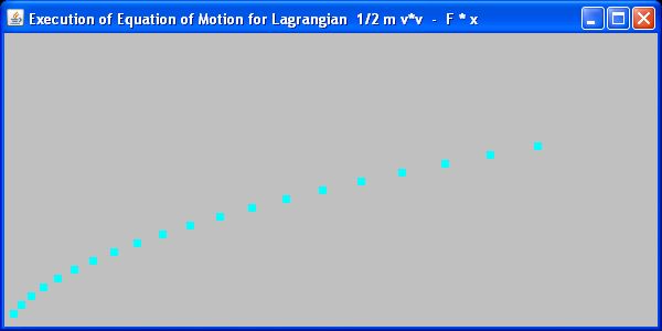
Figure 1: CA run for $L=\frac{1}{2}m\dot{x}^{2}-V(x)$.

The basic Lagrangian mechanism, as originally introduced by Lagrange, defines

$L=T-V$
where T = kinetic energy, V = potential energy. As described in section 2.3, the Euler-Lagrange equation allows the generation of the equation of motion

$m\ddot{x}=\frac{\delta V}{\delta x}$.
To execute the CA, initial settings are required for all entities (and certain derivatives of these entities) appearing in the equation of motion. Setting the initial (and constant) value for $\frac{\delta V}{\delta x}=F$, i.e., assuming a constant power F, leads to the execution of

$F=m\ddot{x}$
for the specified initial values. An example is illustrated in Fig. 1.
Instead of specifying $\frac{\delta V}{\delta x}=F$ it is also possible to initialize the potential V(x) explicitly by a specific spatial distribution and initial values for all CA cells $\{s_{1},...,s_{n}\}$. This enables more general multi-dimensional modeling.

3.2 Harmonic Oscillator

A particle of mass m undergoing simple harmonic motion is described by the Lagrangian

$L=T-V=\frac{1}{2}m\dot{x}^{2}-\frac{1}{2}kx^{2}$ (see, for example, [18], page 25).
The Euler-Lagrange equation leads to

(a) $\frac{d}{dt}\frac{\delta L}{\delta\dot{x}}=\frac{d}{dt}\frac{\delta(\frac{1}{2}m\dot{x}^{2}-V(x))}{\delta\dot{x}}=\frac{d}{dt}\frac{\delta(\frac{1}{2}m\dot{x}^{2})}{\delta\dot{x}}-\frac{d}{dt}\frac{\delta(\frac{1}{2}kx^{2})}{\delta\dot{x}}=\frac{d}{dt}(m\dot{x})=m\ddot{x}$

(b) $\frac{\delta L}{\delta x}=\frac{\delta(\frac{1}{2}m\dot{x}^{2}-V(x))}{\delta x}=\frac{\delta(\frac{1}{2}m\dot{x}^{2})}{\delta x}-\frac{\delta(V(x)}{\delta x}=0-\frac{\delta V}{\delta x}=-kx$
Equating (a) to (b) gives the equation of motion

$m\ddot{x}=-kx$.

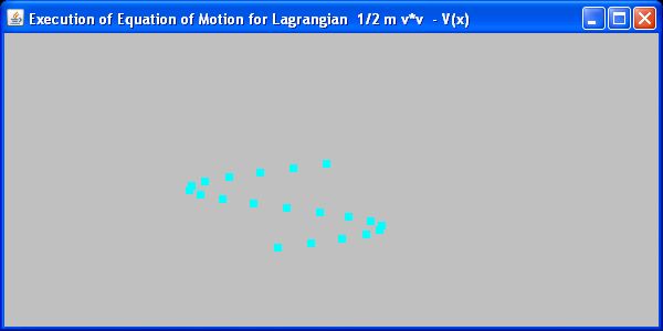
Figure 2: CA run for harmonic oscillator $L=\frac{1}{2}m\dot{x}^{2}-\frac{1}{2}kx^{2}$ .

With [20] the equation of motion for the harmonic oscillator is

$d^{2}z/dt^{2}=-K/M(z-z0)$ $\Rightarrow d^{2}x/dt^{2}=-K/Mx+K/M\cdot x0$

$\Rightarrow d^{2}x/dt^{2}=-K/M\cdot x$ (in case x0 = 0).

Fig. 2 shows a snapshot of running QFTCA with the Lagrangian for the harmonic oscillator $L=\frac{1}{2}m\dot{x}^{2}-\frac{1}{2}kx^{2}$ .

3.3 Waves

The standard formulation of the ”wave equation”, i.e., the equation of motion for waves, is (see, for example [23])

(3) $(\frac{1}{v^{2}}\frac{d^{2}}{dt^{2}}-\frac{d^{2}}{dx^{2}})\psi(x,t)=0$.
The three-dimensional version is

(4) $(\frac{1}{v^{2}}\frac{\partial^{2}}{\partial t^{2}}-\bigtriangledown^{2})\psi(x,t)=0$.
Depending on the particular context, the equation may be varied or extended by setting the right hand side not equal to 0. For example, in [20] the equation of motion for class 1 waves is

(5) $d^{2}\psi/dt^{2}-c_{w}^{2}d^{2}\psi/dx^{2}=–(2\pi\nu)^{2}(\psi-\psi_{0})$.
To obtain the CA update-function, the equation of motion has to be transformed into a sequence of computation steps, including the replacement of the differential operations by discrete ”$\Delta$-units”. The following computation steps for the CA are derived from equation (3) for the state transition $\psi(x_{i},t_{j})\rightarrow\psi(x_{i},t_{j+1})$

1. $t_{j+1}=t_{j}+\Delta t$

2. $\Delta\psi dx=(\psi(x_{i+1},t_{j})-\psi(x_{i-1},t_{j}))/2\Delta x$

3. $\Delta^{2}\psi dx=(\psi(x_{i+1},t_{j})-2\psi(x_{i},t_{j})+\psi(x_{i-1},t_{j}))/\Delta x/\Delta x$

4. equation of motion derived from (3): $\Delta^{2}\psi dt=v^{2}\Delta^{2}\psi dx$

5. $\Delta^{2}\psi dt=(\psi(x_{i},t_{j+1})-2\psi(x_{i},t_{j})+\psi(x_{i},t_{j-1}))/\Delta t/\Delta t\rightarrow$
   $\psi(x_{i},t_{j+1})=\Delta^{2}\psi dt\cdot\Delta t\cdot\Delta t+2\psi(x_{i},t_{j})-\psi(x_{i},t_{j-1})$

Here and subsequently, the following naming conventions are used for going from the differential units to $\Delta$ -units: $d\psi/dt\rightarrow\Delta\psi dt$, $d\psi/dx\rightarrow\Delta\psi dx$, $d^{2}\psi/dx^{2}\rightarrow\Delta^{2}\psi dx$, $d^{2}\psi/dt^{2}\rightarrow\Delta^{2}\psi dt$.

The above sequence of CA computation steps can be generalized and is applicable to arbitrary Lagrangians, except for the Lagrangian-specific step 4. The computation requires an equation of motion that delivers $\frac{d^{2}\psi}{dt^{2}}$ and an initial system state that contains initial values for $\psi(x,t_{0})$ and $\psi(x,t_{-1})$ (or, alternatively, $\Delta\psi dt$) for the relevant positions x. The CA execution has to start with an initial state that represents a specific physical situation.

Notice that the Lagrangian and thus the system state of the CA does not include variables that are usually included in physics theories of waves such as frequency, amplitude, wavelength and energy. These variables are implied by the initial state of the wave and explicitly supported by the CA only if they appear in the equation of motion. Such hidden variables may also appear in the constraints for the initial state mentioned in 2.3.

Fig.3 shows a snapshot from the dynamical evolution of a wave according to the equation of motion $(\frac{1}{v^{2}}\frac{d^{2}}{dt^{2}}-\frac{d^{2}}{dx^{2}})\psi(x,t)=0$ and a suitable initial state.

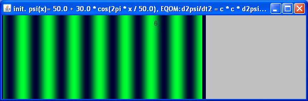
Figure 3: CA run for wave $(\frac{1}{v^{2}}\frac{d^{2}}{dt^{2}}-\frac{d^{2}}{dx^{2}})\psi=0$

3.4 Fields

Fields are based on waves. As with waves (section 3.3), instead of the position variables $x$, $\dot{x}$ and $\ddot{x}$ of the particles, the Lagrangian and related system state contain the entities $\psi(x,t)$ assigned to spacetime points (x,t). The Lagrangian (and the equation of motion) typically depends on $\psi(x,t)$ and the derivatives $\partial\psi/\partial t,\partial\psi/\partial x,\partial^{2}\psi/\partial t^{2},\partial^{2}\psi/\partial x^{2}$.

The equation of motion (which is also called the field equation) is obtained by using the EL equation (1) or by minimizing the action. Depending on the type of field considered, $\psi(x,t)$ may be complex and may represent a vector, matrix, or tensor. The Lagrangian may also describe multiple fields, which means that multiple field variables such as $\psi_{1},\psi_{2}$ or $\varphi_{1},\varphi_{2}$, … may be required.
For fields, the Lagrangian density $\mathcal{L}$ is defined such that

$L=\int\mathcal{L}d^{3}x$ (see [24], pages 16, 17).
In [1] (page 26), the following requirements for Lagrangian density are listed:

1. The Lagrangian density must be a function of the dynamical variables only, i.e., a function of the fields $\psi(x,t)$ and their derivatives.

2. It must not contain any explicit dependencies on the coordinates x.

3. The dependency must be local, i.e., it must depend on $\psi(x,t)$ and partial derivatives of $\psi(x,t)$. To obtain an equation of motion with less than third order derivatives, the derivatives of $\psi(x,t)$ should not be higher than first order.

4. The Lagrangian density must be a real number.

5. A number of symmetry requirements hold. For relativistic theories, the most important symmetry requirement is the requirement for Poincare invariance.

These requirements apply primarily to the Lagrangian of the respective physics theories. For the mapping of the Lagrangian to a cellular automaton the requirements represent an alleviation rather than a problem because they reduce the generality.

3.5 Non-relativistic Quantum Mechanics

In non-relativistic quantum mechanics (QM), the equation of motion is the Schrödinger equation. For a particle moving in one direction, it is

(6) $-\frac{\hbar^{2}}{2m}\frac{\partial^{2}\psi(x,t)}{\partial x^{2}}+V(x,t)\psi(x,t)=i\hbar\frac{\partial\psi(x,t)}{\partial t}$.
The update-function of the CA continuously determines $\frac{\partial\psi}{\partial t}$ as to

(7) $\frac{\partial\psi}{\partial t}=\frac{V\psi}{i\hbar}-\frac{\hbar}{2mi}\frac{\partial^{2}\psi}{\partial x^{2}}$.
Because the equation of motion delivers $d\psi/dt$ instead of $d^{2}\psi/dt^{2}$ described in section 3.3 for waves, the computation sequence shown in section 3.3 for the state transition $\psi(x_{i},t_{j})\rightarrow\psi(x_{i},t_{j+1})$ is slightly varied to become

1. $t_{j+1}=t_{j}+\Delta t$

2. $\Delta\psi dx=(\psi(x_{i+1},t_{j})-\psi(x_{i-1},t_{j}))/2\Delta x$

3. $\Delta^{2}\psi dx=(\psi(x_{i+1},t_{j})-2\psi(x_{i},t_{j})+\psi(x_{i-1},t_{j}))/\Delta x/\Delta x$

4. equation of motion derived from (7): $\Delta\psi dt=\frac{V\psi}{i\hbar}-\frac{\hbar}{2mi}\Delta^{2}\psi dx$

5. $\Delta\psi dt=\Delta\psi dt+\Delta^{2}\psi dt\cdot\Delta t$

6. $\psi(x_{i},t_{j+1})=\psi(x_{i},t_{j})+\Delta\psi dt\cdot\Delta t$

The naming conventions are those described in section 3.3. With quantum theory $\psi(x,t)$ is a complex scalar number.

Many laws of quantum mechanics that are usually described in textbooks for QM cannot directly be deduced from the Schrödinger equation (or the related Lagrangian). Major examples are the uncertainty relation, the rules explaining the double slit experiment and the measurement problem. As a consequence, it is not possible to derive a CA that supports full QM purely from the Schrödinger equation. The author claims that a major part of the required additional specifications can only be provided by a functional model of QT that includes QT interactions. In [3], such a functional model of QT interactions is proposed and is the basis for section 5.

4 Quantum Fields and Particles

Compared to (non-relativistic) quantum mechanics, quantum field theory is a relativistic theory of quantum fields and particles and interactions among fields and particles. Particles are largely treated like fields. In the literature, for example, [20], particles are called ”quanta of fields”. Various field types with differing Lagrangians are distinguished. For the purpose of this paper, it is sufficient to consider the field(s) of quantum electrodynamics (QED). In [18] (page 170), the Lagrangian of QED is given by

$L_{QED}=L_{EM}+L_{Dirac}+L_{int}$
with

$L_{EM}=-\frac{1}{4}F_{\mu\nu}F^{\mu\nu}$

$L_{Dirac}=i\bar{\psi}\gamma^{\mu}\partial_{\mu}\psi-m\bar{\psi}\psi$

$L_{int}=-q\bar{\psi}\gamma^{\mu}\psi A_{\mu}$.
Thus

(8) $L_{QED}=-\frac{1}{4}F_{\mu\nu}F^{\mu\nu}+i\bar{\psi}\gamma^{\mu}\partial_{\mu}\psi-m\bar{\psi}\psi-q\bar{\psi}\gamma^{\mu}\psi A_{\mu}$
The equations refer to two types of fields: the electromagnetic field and the Dirac field. Leaving aside interactions between fields and particles (which will be addressed in section 5), it is sufficient to consider the equations of motion for the individual field types and particle types separately. The equations of motion can be derived directly from the respective Lagrangian parts. For example, the equation of motion (called the field equation) for the Dirac field, the so-called Dirac equation, is

(9) $i\hbar\gamma^{\nu}\frac{\partial_{\psi}}{\partial x^{\nu}}-mc\psi=0$.
Thus, a QFTCA that supports QFT, or a specific part of QFT, such as QED, has to have different update-functions depending on the different field types and particle types to be supported. Additionally, the system state encompassing physics objects and cell states depends on the field types and particle types.

CA applications with multiple fields and/or particles may be viewed as the union of multiple independent field-specific CAs (as long as interactions are disregarded).

5 Interacting Quantum Fields and Particles

This section considers interactions among particles and interactions between particles and fields. The considerations focus on interactions between two ”in” particles resulting in one or two ”out” particles. Only interactions are considered, which, in QFT, are dealt with by scattering matrices and Feynman diagrams (in [3] and in the following such interactions are called ”QFT interactions”).

Many details of QFT concerning interacting particles/fields can be derived from the interaction part of the Lagrangian. For QED, the interaction part of the Lagrangian in equation (8) is

(10) $L_{int}=-q\bar{\psi}\gamma^{\mu}\psi A_{\mu}$
In contrast to the areas described in the preceding sections, a functional model of QFT interactions cannot solely be derived from the Lagrangian. Additional assumptions have to be specified to obtain a complete functional model for QFT interactions. In [3], such a functional model of QFT interactions is described and is taken as the basis for the CA-based functional model described in the present section. The following is a summary of the functional model of QFT interactions as described in [3], mapped to the structure and concepts of QFTCA and partly providing more details in terms of QFTCA.

5.0.1 Refinement of the system state structure

To support a CA-based functional model of QFT interactions the system structure described in section 2.2 has to be refined.

QFT provides an extensive framework for the more detailed evaluation of probability amplitudes for various types of interactions. This framework is based on Feynman diagrams and related ”Feynman rules”. Rules have been established for the derivation of the possible Feynman diagrams from a given Lagrangian.

With QFT (see, for example, [21]), an interaction (e.g., scattering) is described by the scattering matrix (S-matrix), which assigns a probability amplitude $S_{\beta\alpha}$ to the transition of a given ”in” state $\Psi_{\alpha}$ to an ”out” state $\Psi_{\beta}$.
$S_{\beta\alpha}=(\Psi_{\beta},\Psi_{\alpha})$
The ”in” and ”out” states are specified by their state components
$\Psi_{\alpha}=\{inparticle1(p1,\sigma 1,n1),inparticle2(p2,\sigma 2,n2)\}$;
$\Psi_{\beta}=\{outparticle1(p1^{\prime},\sigma 1^{\prime},n1^{\prime}),outparticle2(p2^{\prime},\sigma 2^{\prime},n2^{\prime})\}$.
Here, $p_{i}$ represents the momentum, $\sigma_{i}$ is the spin, and $n_{i}$ is the particle type. For a more complete specification of a state, the position x and the time t are also part of the state. For the computation of a QFT scattering matrix element, a concrete in-state $\Psi_{\alpha}$ and a concrete out-state $\Psi_{\beta}$ are typically assumed. For a functional model of QFT, however, the dynamical evolution of the system state does not end with a concrete and definite interaction result but may continue with a multitude of alternative interaction results. Only a measurement (by use of other QFT interactions) reduces the multitude of possible scattering results to a single definite result. Thus, for a functional model, the complete interaction result consists of all the possible out-state combinations with associated probability amplitudes.
$outstate=\{$
$\{amplitude_{1},outparticle1(t,x1_{1},p1_{1},\sigma 1_{1},n1),outparticle2(t,x2_{1},p2_{1},\sigma 2_{1},n2)\}$,
$\{amplitude_{2},outparticle1(t,x1_{2},p1_{1},\sigma 1_{2},n1),outparticle2(t,x2_{2},p2_{2},\sigma 2_{2},n2)\}$,
…
$\{amplitude_{i},outparticle1(t,x1_{i},p1_{i},\sigma 1_{i},n1),outparticle2(t,x2_{i},p2_{i},\sigma 2_{i},n2)\}$,
…
}
This interaction result suggests a huge multitude of state combinations (with associated probability amplitudes). The multitude is reduced due to two points:

1. Only specific combinations of outparticle1() and outparticle2() are possible (for example, because of energy and momentum conservation).
   (outstate is not a product state of outparticle1-state and outparticle2-state).

2. Only a discrete set of alternative out states (called ”paths”) is assumed with the CA-based functional model.

In [3], the above state structure, which represents the interaction results, is called a particle/wave-collection (pw-collection). A tabulated representation of a pw-collection is shown in Table 1.

Table 1: Structure of a pw-collection consisting of two particle/waves pw1 and pw2 and N paths.

paths	pw1-state	pw2-state	amplitude
path-1	pw1-state1	pw2-state1	ampl-1
path-2	pw1-state2	pw2-state2	ampl-2
…	…	…	…
path-N	pw1-stateN	pw2-stateN	ampl-N

5.0.2 Occurrence of interaction

In terms of wave equations (i.e., the equations of motion for waves) (see [20]), an interaction between two waves $\psi_{1}$ and $\psi_{2}$ resulting in a third wave $\psi_{3}$ is described by an equation of motion in which the product of waves $\psi_{1}$ and $\psi_{2}$ is related to $\psi_{3}$ as, for example,

$d^{2}\psi_{3}/dt^{2}-c^{2}d^{2}\psi_{3}/dx^{2}=a^{2}\psi_{3}+b\cdot\psi_{1}\psi_{2}$
(Typically, similar equations exist defining the interactions between $\psi_{1}$ and $\psi_{3}$ and between $\psi_{2}$ and $\psi_{3}$.)
An interaction occurs if, for a position $x_{0}$ the product $\psi_{1}(x_{0},t)\cdot\psi_{2}(x_{0},t)$ becomes non-zero, which means that both $\psi_{1}$ and $\psi_{2}$ have to be non-zero.

In terms of a CA-based model, such as QFTCA, an interaction occurs if, for a cell $c_{0}$, two fields $\psi_{1}$ and $\psi_{2}$ have a non-zero value. This appears to be trivial, but it does not specify what occurs if, at a given CA-update cycle, multiple cells satisfy this condition. In line with the functional model of QFT interactions described in [3], the following mechanism is assumed with QFTCA:

• Only one single (discrete) position (i.e, CA cell) may cause an interaction and the interaction results depend on the state attributes associated with this position.

• In general, a QFT interaction results in the creation of new ”out” particles/waves (which may be of the same types as the ”in” particles/waves). This may be viewed as a ”collapse of the ingoing particle/wave” and a reduction of the ”in” particles/waves to the definite attribute values associated with the interaction position.

• If multiple positions (i.e., cells) satisfy the condition for the occurrence of an interaction, the single interaction position is randomly (i.e., non-deterministically) selected as a function of the probability amplitudes of the candidate cells/positions.

This mechanism enables a modeling of QFT interactions (e.g., scatterings). It also offers a model of QT measurement in which measurements are realized by ”normal” QFT interactions (see also section 6.5). After an interaction has been initiated (and the occurrence of multiple interactions of the same type has been blocked), the interaction process is performed. In [3], the interaction process is subdivided into the three process steps. These process steps have to be performed as part of the CA update-function:

perform-interaction ::= {
  Step0: Occurrence of interaction;
  Step1: Formation of interaction-object;
  Step2: Formation and processing of interaction channels;
  Step3: Generation of "out" particle/waves.
}

5.0.3 Formation of interaction object

At the beginning of a QFT interaction, the information from the interacting particles/waves is merged into an ”interaction object”. At the end of the interaction, the interaction object is replaced by the the ”out” particles/waves.

The functional model assumes that interaction objects, similar to virtual particles, have a limited life-time before they decay into the ”out” particles/waves that are the result of the interaction. In contrast to virtual particles, the interaction object does not correspond to a single real particle, but contains the information from both interacting particles.

5.0.4 Formation and processing of interaction channels

Starting with the interaction object, the CA update-function continues with the determination of the probability amplitudes for the possible results of the QFT interaction. In standard QFT the computation of the probability amplitudes is based on Feynman diagrams, rules (called Feynman rules) and the assumption of ”virtual particles”. The CA update-function (of course) cannot use Feynman diagrams for the computation of state transitions toward the interaction results. Instead, the functional model of QFT interactions assumes interaction channels.

Interaction-channels are generated according to rules that are equivalent to the Feynman rules for the generation of Feynman diagrams. Like the Feynman rules, the interaction-channel generation rules are related to the interaction part of the Lagrangian (or the equation of motion). As an example, consider the interaction part of the QED Lagrangian, which in equation (10) is given by

$L_{int}=-q\bar{\psi}\gamma^{\mu}\psi A_{\mu}$.
Here, $\psi$ represents the electron field, $\bar{\psi}$ is the positron field, and $A$ is the photon (i.e., electromagnetic) field. Thus, the equation applies to interactions between electrons $e^{-}$, positrons $e^{+}$, and photons $\gamma$. The interaction is expressed in terms of creation and annihilation operators by

(12) $H_{W}(x)=-eN\{(\bar{\psi^{+}}+\bar{\psi^{-}})(\not A^{+}+\not A^{-})(\psi^{+}-\psi^{-})\}_{x}$
where $\bar{\psi^{+}},\bar{\psi^{-}},\not A^{+},\not A^{-},\psi^{+},\psi^{-}$ are creation and annihilation operators. This includes four variants of photon absorption, $e^{-}+\gamma\rightarrow e^{-}$, $e^{+}+\gamma\rightarrow e^{+}$, $e^{-}+e^{+}+\gamma$, $\gamma\rightarrow e^{-}+e^{+}$ and four variants of photon emission, $e^{-}\rightarrow e^{-}+\gamma$, $e^{+}\rightarrow e^{+}+\gamma$, $e^{-}+e^{+}\rightarrow\gamma$, $\rightarrow e^{-}+e^{+}+\gamma$ ( see [17], page 111).

Each interaction-channel starts with both ”in” particles/waves and ends with ”out” particles/waves. Alternative interaction-channels may differ in the set of ”out” particles/waves and/or in the sub-channels between the ”in” and ”out” particles/waves.

A specific interaction-channel is formed by the combination of the two operators split() and combine().

split(a) $\rightarrow$ (b,c) means that split(a) results in b and c;

combine(a,b)$\rightarrow$ (c) means that combine(a,b) results in c.
For example, starting with two interacting particles/waves pw1 and pw2, the interaction-channel specified by
(pw1,pw2): split(pw1) $\rightarrow$ (a,b); combine( a, pw2 ) $\rightarrow$ ( c)
would result in ”out” particles/waves b and c.

The split() and combine() operators are analogous (although not equal) to the creation and annihilation operators of QFT. Derived from QFT, the following rules are established for the functional model of interactions:

• Rule1: An interaction always starts with two ”in” particles/waves and ends with two ”out” particles/waves.

• Rule2: An interaction-channel always contains one combine() and one split() (in arbitrary sequence).

Given the above rules, there are five possible interaction-channels that can be constructed from the two interacting particles/waves pw1 and pw2:

1. combine( pw1, pw2 ) $\rightarrow$ (a) split(a) $\rightarrow$ (b,c)

2. split(pw1) $\rightarrow$ (a,b) combine( a, pw2 ) $\rightarrow$ (c)

3. split(pw1) $\rightarrow$ (a,b) combine( b, pw2 ) $\rightarrow$ (c)

4. split(pw2) $\rightarrow$ (a,b) combine( pw1, a ) $\rightarrow$ (c)

5. split(pw2) $\rightarrow$ (a,b) combine( pw1, b ) $\rightarrow$ (c)

All these interaction-channels end with two particles/waves (a, c) or (b, c). Depending on the type of particles/waves involved in the interaction, QFT supports only specific types of splits and combines. The rules that define what combinations of particle types may be subject to combine(p1, p2) and what the resulting particle types of split(p1) and combine(p1, p2) can be are equivalent to the rules regarding the possible vertices of Feynman diagrams, as described in numerous textbooks on QFT (see for example, [19], [12], [17]). For QED, for example, one of the rules is split( $\gamma)\rightarrow(e^{-},e^{+})$; combine($e^{-},\gamma)\rightarrow(e^{-})$ .
Sometimes QFT rules allow for multiple results for split() and combine(). For example, split(photon) may result in (electron, positron), (muon, antimuon), or (tauon, antitauon). Finally, with specific ”in” particle/wave combinations, it may turn out that some of the possible interaction-channels may be considered equivalent, and therefore only one of them has to be included. Given the QFT rules, typically only one or two of the above mentioned five alternative interaction-channels are possible for a specific ”in” particle combination.

The operator split(a) $\rightarrow$ (b, c) is a non-bijective function insofar, as there are many alternatives with respect to the attributes (e.g., momentum and spin) of the resulting (b, c). Rather than selecting a particular specific result, QFT (and the functional model of QT interactions) requires that a multitude of possible results are generated with differing probability amplitudes assigned. Thus, split(a) $\rightarrow$ (b, c) results in a two-fold splitting and may be expressed as

split(a) $\rightarrow((b_{1},c_{1}),(b_{2},c_{2}),...(b_{n},c_{n}))$.
For the interaction object this means that a multitude of paths representing $((b_{1},c_{1}),(b_{2},c_{2}),...(b_{n},c_{n}))$ have to be generated. As a consequence, at the end each interaction-channel contains a multitude of paths because each interaction-channel includes a split() operator. The alternative interaction-channels that are generated by the varying application of the split() and combine() operators are processed in parallel. The effects of processing the split() and combine() operators is reflected in extensions of and changes in the interaction object.

The rules governing the computation of the amplitudes of a path of an interaction object must be in accordance with QFT. These rules are well known and described in many textbooks on QFT (see for example, [19], [12], [17]). However, with QFT the respective rules are defined in terms of (external and internal ) lines and vertices of Feynman diagrams. For the functional model, the QFT rules have been mapped to rules regarding the split() and combine() operators.

5.0.5 Generation of ”Out” Particles/Waves

The processing of the interaction channels ends with a certain ”out” particle/wave combination. With some types of interactions, different ”out” particle/wave combinations may occur. The functional model of QT interactions assumes that from the possibly multiple alternative ”out” particle/wave combinations only one will actually leave an interaction.

After processing the individual interaction channels (in parallel), each interaction channel contains the same set of paths, however, with different probability amplitudes for the paths. Therefore, the multiple interaction channels can be (re-)united by the summation of the corresponding amplitudes. According to QFT rules (usually formulated in terms of Feynman diagrams), the ”summation”, in some cases, has to be performed with a negative sign (i.e., $amplitude1-amplitude2$ instead of $amplitude1+amplitude2$).

5.0.6 More detailed mapping of the process steps and the system state to QFTCA

In the above sections a relatively rough description of the CA-based functional model of QFT interactions is given. Disregarding the size limitations for the present paper, additional, more detailed specifications would be desirable for the mapping of (1) the interaction process steps to CA-update functions and (2) the related system state to CA cells. As the simplest and initial solution it can be assumed that the whole interaction (with the above described four process steps) is performed during a single invocation of the update function and that, except for the elimination of non-interacting paths; this process affects only a single cell until the interaction results are generated. As a next level of refinement, it is imaginable that parts of the interaction process, such as the split() and combine() operators, can be mapped to the CA-based model of waves and fields, as described in sections 4 and 5. This author’s computer model (see [2] has the objective to support the development of further model refinements.

5.0.7 Overall Properties of QFT Interactions

With the above described functional model of QFT interactions, the function ”QFT-interaction()” does not constitute a bijective mapping. Step 0, ”Occurrence of interaction”, does not provide a surjective mapping; only one of the multiple ”in” particle positions is mapped to the interaction result. Step 3, ”Generation of ”out” particles/waves”, does not represent an injective mapping; multiple ”out” paths with non-zero probability amplitudes are generated such that the ingoing state could only partly be reconstructed from the ”out” state. Altogether, the interaction process implies a non-bijective mapping. As described in section 6.5, this non-bijective mapping associated with QFT interactions offers an explanation for part of the limitations and peculiarities of QT measurement.

6 Discussions

6.1 How complete is the Lagrangian for the formulation of a physics theory

The Lagrangian (and related constructs such as the Hamiltonian and the equation of motion) is an impressively powerful basis for the formulation of theories of areas of physics. Many details of existing physics theories can be derived from the Lagrangian. Many past findings in physics theories have been developed by considerations of the Lagrangian (mostly symmetry considerations). Nevertheless, the Lagrangians do not completely specify physics theories. As shown in this paper, mainly two additional aspects are required to enable the construction of a comprehensive CA-based functional model that reflects subject physics theory.

1. Initial states for the execution of the equation of motion
   The Lagrangian and equations of motion are typically differential equations. As a trivial matter of mathematics, to obtain solutions for the differential equations or a model that shows the dynamical evolution of a system, some initial state (i.e., initial values for the differential equation) has to be assumed. As shown with the sample areas of physics (sections 3, 4 and 5), however, it is not sufficient to select arbitrary initial states. Typically, various types of constraints exist for the initial state. Only part of these constraints can be derived from the Lagrangian. Further constraints have to be derived from the full physics theory as described in related textbooks.

2. Process models of physics theories
   As described in section 1, a cellular automaton may be viewed as a specific type of a ”functional model” (or ”process model”), i.e., a model that specifies the dynamical evolution of the system in terms of state transitions. With classical areas of physics, such as Newtonian mechanics (see section 3.1), such a process model in the form of a CA can be derived from the Lagrangian. With more advanced physics theories, additional statements are required for the specification of the dynamical evolution of a system. Partly, these additional statements can be found in textbooks of the respective physics theories. Partly, the required additional statements are still missing or still debated among physicists. The major subject in which the provision of a process model (here, in the form of a CA) requires additional specifications is the area of interactions in quantum field theory (section 5).

6.2 The role of non-local information

The dynamical evolution of the classical CA depends exclusively on information that can be assigned to the CA cells, and the update-function for a cell depends only on the contents of the neighbor cells (including the respective cell). This cell-related information is here called ”local information”. Differing from classical CAs, the system state of QFTCA described in this paper contains, in addition to the cell-related (local) information, non-local information pertaining to the physical objects (e.g., fields and particles). While originally the inclusion of the non-local information was merely justified by the goal to obtain a decent model, it turned out that the inclusion of non-local information to represent physical objects spanning larger areas of cell-space is key for the modeling of non-local effects in connection with QFT interactions (see section 5). Non-local effects, such as the collapse of the wave function and entanglement, can best be explained by the assumption of physical objects with non-local attributes and actions (see below, section 6.5 Measurement).

6.3 The special role of time in the CA-based model

Deviating from the trend in physics theories to treat space dimensions and the time dimension, as much as possible, on equal footing, the Lagrangian-based CA described in this paper assumes a special role of time with several aspects:

1. Time is not a fourth dimension of the CA,
   Instead, QFTCA maintains only a single time slice (i.e., the current time slice). As described in section 2, this implies that the time derivatives appearing in the equation of motion (e.g., $d\psi/dt$, $d^{2}\psi/dt^{2}$ ) have to be kept explicitly as part of the system state. While this may be viewed as just a type of implementation decision for the QFTCA, it also supports the author’s goal to show that models for the evolution of our universe that assume only a single time layer are at least feasible.

2. The existence of a time arrow
   The goal of providing a functional model, such as a CA-based model, of a physics theory may be viewed as presupposing causality and an arrow of time. Insofar, it should not be a surprise that the QFTCA described in this paper implies an arrow of time. The neutrality with respect to a direction of time that is represented in the (declarative) equations of physics theories, such as the Lagrangians, is necessarily lost with the construction of a functional (e.g., CA-based) model.

6.4 Consequences of discreteness

One of the key properties of CA-based models is discreteness with respect to space and time. Discreteness with respect to space and time coordinates may cause discreteness with respect to further aspects, such as, for example, momentum. Two questions arise: (1) whether discreteness impedes the precise modeling of physics theories and (2) to which extent discreteness enables new solutions in areas that are not yet completely understood.

6.4.1 Does discreteness impede the precise modeling of physics theories?

To achieve compatibility with the predictions of the standard formulations of physics theories, the granularity of the space and time coordinates has to be sufficiently fine. It can be expected that the finer the granularity is, the better the agreement of the results of the CA-based modeling is with the results predicted by the theories and the results measured in experiments. It can also be expected (and has been confirmed by the author’s computer simulations) that an insufficiently fine granularity may, in some cases, result in chaotic (i.e., unpredictable) behavior of the CA. A conclusive answer to the above question requires more complete computer modeling from the author.

6.4.2 Does discreteness enable new solutions?

Discreteness may result in non-linear and even unpredictable behavior (especially if there is insufficiently fine granularity). This leads to the question of whether the discreteness of the CA may provide an explanation for the non-determinism of QT. The author’s work in this area (including the computer model QFTCA, see [2]) has so far not resulted in a final answer to this question. While it is easy to generate unpredictability, it has been (so far) not possible to generate through discreteness unpredictability that adheres to the laws of QT.

As a further application of discreteness, the functional model of QFT (see [3]), which is also the basis for the CA-based model described in section 5, assumes discreteness with the paths of a particle. This enables a functional model of QFT interactions that offers a new solution for the non-linearity associated with the collapse of the wave function (see section 5) and QT measurement (see [4] and section 6.5 below).

6.5 QT measurement

In [4], a functional model of QT measurement is described with the following key characteristics:

1. A measurement always implies interactions between the measured quantum object and the measurement environment.
   Measurements of QT observables can be performed using a variety of measurement devices, apparatuses, and processes. All such measurement processes have to include at least one interaction in which the measured object exchanges information with some other entity belonging to the measurement apparatus.

2. The model of measurement interactions is based on QFT interactions, as described in section 5.
   The model assumes that the interactions between the measured QT object and the measurement apparatus are ”normal” interactions that adhere to the laws of quantum field theory.

3. In general, the interacting particles/waves consist of multiple ”paths” with different associated probability amplitudes. The interaction always occurs at a definite position. Only the paths that cover the interaction position determine the result of the (measurement) interaction.

4. The measurement process includes a collapse of the wave function.
   After the interacting paths are determined and used to generate the interaction result (i.e., measurement result), all of the remaining paths are discarded. This may be considered as the ”collapse of the wave function”.

5. As described in section 5, QFT interactions support only a non-bijective mapping of the ”in” state to the ”out” state and thus only the limited exchange of information. This limited exchange of information is the cause of some of the limitations and peculiarities of QT measurements.

The QFTCA described in the present paper (section 5) supports the functional model of QT measurement described in [4] and adds further details to item (3) (definite interaction position) and item (4) (collapse of the wave function).

6.6 The linearity/non-linearity of QFTCA

Linearity is a very important feature of QT. It is therefore reasonable to discuss the linearity/non-linearity of CAs in general and of QFTCA specifically. In [6], [7] and [8], H-T. Elze discusses the general linearity/non-linearity of CAs in detail. As a supplement to the findings described in [6], [7] and [8], the findings of the author using the computer model of QFTCA (see [2]) show that an insufficiently fine granularity of the discreteness of a CA may cause a theoretically linear process to become non-linear or even chaotic. For QFTCA specifically, the preservation of linearity is not considered an issue. QFTCA is seen as a type of ”implementation” of an underlying theory (primarily QFT). Where the underlying theory requires linearity, QFTCA must provide linearity. There are, however, two areas where QFT, the theory underlying QFTCA, does not define sufficient detail for a CA implementation; therefore, the solution(s) chosen by QFTCA may potentially violate linearity. The two aforementioned areas are the following:

1. The collapse of the wave function
   The request for the linearity of QT applies to the normal progression of the quantum system as described by the laws of QT. However, the laws of QT (in particular the equations of motion, e.g., the Schrödinger equation) describe only the evolution of probabilities and probability amplitudes. For the transition of the probabilities to facts (i.e., the measurement), there does not yet exist a generally agreed-upon theory. Ideas and proposals for a theory on measurement often assume the collapse of the wave function. Theories of the collapse of the wave function have a tendency towards non-linear solutions (see, for example, [10] and [5]). QFTCA is based on the functional model of QT interactions described in [3], which also assumes a collapse of the wave function. Differing from the theories described in [10] and [5], which achieve non-linearity by modifications of the differential equations of the equation of motion, the functional model of QT interactions, as represented by QFTCA, utilizes the power and flexibility of functional descriptions to achieve the desired discontinuity associated with the collapse of the wave function.

2. QFT interactions
   As described in section 6.5., QFTCA assumes that normal QFT interactions may represent a measurement and that, therefore, normal QFT interactions may contain a collapse of the wave function. Thus, to which extent QFT interactions may represent non-linearities (in case they include a collapse of the wave function) must be discussed.

   In QFT, an important construct for the treatment of QFT interactions is the scattering matrix (S-matrix). In [21], Weinberg states that the S-matrix has been proven to be a unitary matrix. This characteristic of the S-matrix is often seen as a proof that QFT interactions obey linearity. However, the scattering matrix is not the equation of motion of QFT interactions. As described in sections 5, the QFT interaction does not perform a bijective mapping of the ”in” state to the ”out” state. Whether or not this may still be considered to be a linear progression of the equation of motion is not clear to the author.

To summarize, it is not clear whether the above-mentioned potential non-linearities indeed represent non-linearities, and if they do, whether these non-linearities are already present within the underlying QFT is also unclear. H-T. Elze showed in [8] that modifications in the underlying equation of motions may result in non-linearities. QFTCA does not assume a modification of the underlying equations of motion (or Lagrangian or Hamiltonian) but adds some interpretation details to enable the generation of a functional model.

6.7 Entanglement

The functional model of QT measurement described in [3] includes a model on entanglement. The basic assumption is that the paths that represent alternative measurement outcomes, even with normal QFT interactions (see section 5.3), encompass both correlated particles/waves. When a measurement (i.e., a QFT interaction) selects a single path for the interacting particle/wave, the selection also determines a specific correlation. This mechanism is not further addressed in the present paper.

7 Summary and Conclusions

This paper describes an exercise to construct models of areas of physics in terms of a cellular automaton and to derive these models (i.e., the concrete CA), as much as possible, from the Lagrangian of the respective physics theory. Because it was not expected that the classical CA is sufficient to model all areas of physics, nor that the Lagrangian alone is sufficient to derive complete functional models of the physics theories, a further aim of the exercise was to determine where the respective limitations are and how they can be overcome with extensions (of the CA) and the additional information required for a complete functional model.

The required extensions to the classical CA resulted in the proposal for a QFTCA described in section 2.2. The most significant extension is the inclusion of non-local physics objects, i.e., objects that span larger areas of cell-space and may overlap.

The Lagrangian and equation of motion provide a powerful basis for the provision of a (CA-based) functional model. For the modeling of advanced areas of physics, such as QT/QFT, however, additional specifications are required. Partly, the additional specifications can be obtained from the subject physics theories as described in textbooks. With QFT, even further specifications, which cannot be derived from the standard formulation of QFT, are required. The functional model of QFT interactions described in [3] has been taken as the basis for the CA-based model described in this paper (section 5 and 6).

In addition to the determination and circumvention of the mentioned limitations, the construction of the Lagrangian-driven CA-based functional model led to a number of issues (see section 6: consequences of discreteness, the role of non-local information, the special role of time, weakening the goal of linearity) that are probably of interest beyond the scope of the present paper. With some of these issues, only preliminary results can be offered by the author. More conclusive answers can probably only be developed through further computer simulations.

Appendix 0.A The Computer Model QFTCA

The computer model QFTCA is an implementation of a cellular automaton which supports the modeling of quantum field theory (QFT). The details of the particular area of QFT (e.g., quantum electrodynamics) are specified by the provision of a Lagrangian and further information related to the Lagrangian. As the major objective, the computer model supports also the modeling of interactions in QFT such as scatterings. The modeling of QFT interactions requires, first at all, some ”functional model” of QFT (i.e. a model which specifies the dynamical evolution of the system in terms of state transitions). Because such a functional model of QFT cannot directly be derived from the existing standard formulation of QFT, this functional model had to be formulated first. The functional model of QFT described in [3] is used as a basis.

0.A.0.1 Input specifications

The primary input is the Lagrangian or the equation of motion of the subject theory. From parameters which appear in the equation of motion further detailed specifications are prompted for

• the number of space dimensions to be supported by the CA,

• the number of particles to be supported,

• details and initial states of the individual particles,

• details and initial states of the fields

• initial values for the other variables which appear in the equation of motion

0.A.0.2 Result of running QFTCA

A QFTCA run shows the dynamical evolution of the system state. Visualization is provided for particle positions and for the probability amplitudes associated with fields and particles.

0.A.0.3 Implementation

Starting with a Lagrangian the equation of motion is determined by use of the Euler-Lagrange equation. This involves differentiation of the Lagrangian. The equation of motion is the basis for the update function of the CA. The equation of motion is typically a differential equation (often second order). In general mathematics, the computation of values $\psi(x,t)$ for fields and particles requires finding solutions for the respective differential equations. QFTCA includes neither a ”general differential equation processor” nor a ”symbolic mathematics engine”. The transformation of the Lagrangian to the equation of motion supports only a small variety of typical Lagrangians. The determination of the dynamical evolution of state variables such as $\psi(x,t)$ does not determine solutions of the differential equations, but interprets the equation of motion in terms of the discrete state variables.

References

- [1] N.N. Bogoliubov, D.V. Shirkov: Quantum Fields, ISBN 0-8053-0983-7 (1982)
- [2] H. Diel: ”QFTCA, a CA-based computer model supporting quantum field theory”, submitted for publication, see ”http://www.hans-diel.de/QFTCA.pdf” (2015)
- [3] H. Diel: ”A functional model of interactions in quantum theory”, arXiv 1405: 6099v2 (2015)
- [4] H. Diel: ”A model of the measurement process in quantum theory”, arXiv1405:5982v1 (2014)
- [5] L. Diosi : ”Is spontaneous wave function collapse testable at all?” , Journal of Physics: Conference Series, Volume 626 (2015)
- [6] H-T. Elze: ”Action principle for cellular automata and the linearity of quantum mechanics”, Phys. Rev. A 89, 012111 (2014), arXiv:1312.1615l, (2013)
- [7] H-T. Elze: ”The linearity of quantum mechanics from the perspective of Hamiltonian cellular automata”, Journal of Physics: Conference Series 504 (2014) 012004, arXiv:1403.2646
- [8] H-T. Elze: ”Are nonlinear discrete cellular automata compatible with quantum mechanics?”, J. Phys.: Conf. Ser. 631, 012069 (2015), arXiv:1505.03764
- [9] E. Fredkin: ”Digital mechanics: An informational process based on reversible universal cellular automata”, Physica D 45, 254-270 (1990)
- [10] G.C. Ghirardi, A. Rimini, T. Weber: ”A Model for a Unified Quantum Description of Macroscopic and Microscopic Systems”. Quantum Probability and Applications, L. Accardi et al. (eds), Springer, Berlin (1985)
- [11] G. Groessing and A. Zeilinger, ”Quantum Cellular Automata”, Complex Systems 2, 197-208, (1988)
- [12] D. Griffiths: Einfuehrung in die Elementarteilchenphysik, Wiley-VCH, 251, 159 (1999)
- [13] G. ’t Hooft: ”The Cellular Automaton Interpretation of Quantum Mechanics”, arXiv:1405.1548v2 ( 2014)
- [14] G. ’t Hooft G ”The Conceptual Basis of Quantum Field Theory”, in Handbook of the Philosophy of Science, Elsevier, 12 (2004)
- [15] A. Ilachinski: Cellular Automata: A Discrete Universe. World Scientific. ISBN 9789812381835, (2001)
- [16] T. D. Lee, Phys. Lett. 122B, 217 (1983); do. J. Statist. Phys. 46, 843 (1987).
- [17] F. Mandl, G. Shaw: Quantenfeldtheorie, AULA Verlag, 351, (1993)
- [18] D.McMahon: Quantum Field Theory Demystified, Mc Graw Hill, (2008)
- [19] L.H. Ryder: Quantum Field Theory, chapter 3, Cambridge University Press, Cambridge (1985)
- [20] M. Strassler: Conversations About Science with Theoretical Physicist M. Strassler, http://profmattstrassler.com/articles-and-posts/particle-physics-basics/Higgs/6. Fields Of Particular Significance.html
- [21] S. Weinberg: Quantum Theory of Fields, Volume 1, Foundations, Cambridge University Press, (2005)
- [22] S. Wolfram: A new kind of science, Wofram Media, ISBN 978-1579550080, (2002)
- [23] C. W. Wong: Introduction to Mathematical Physics, Methods & Concepts, Oxford University Press, (1991)
- [24] A.Zee: Quantum Field Theory in a Nutshell, Princeton University Press (2003)