Hamilton dynamics for the Lefschetz thimble integration akin to the complex Langevin method

Abstract

The Lefschetz thimble method, i.e., the integration along the steepest descent cycles, is an idea to evade the sign problem by complexifying the theory. We discuss that such steepest descent cycles can be identified as ground-state wave-functions of a supersymmetric Hamilton dynamics, which is described with a framework akin to the complex Langevin method. We numerically construct the wave-functions on a grid using a toy model and confirm their well-localized behavior.

A22, A24, B15

1. Introduction.

The first-principle approach to solve the theory is an ultimate goal of theoretical investigations. The quantum Monte Carlo simulation for the functional integral has been a powerful ab initio technique to reveal non-perturbative features of various physical systems. Successful applications include the lattice-QCD (Quantum Chromodynamics) simulation, the lattice Hubbard model, the path integral representation of spin systems, etc.

The Monte-Carlo algorithm is based on importance sampling, so it is demanded that the integrand should be positive semi-definite, i.e., $\mathrm{e}^{S}\geq 0$ where $S$ is the classical action. This positivity condition is often violated in systems of our interest and then we can no longer rely on Monte Carlo simulations (1; 2). In QCD a finite baryon or quark density introduces a mixture of Hermitian and anti-Hermitian terms in the action, and then $\mathrm{e}^{S}$ acquires a complex phase. In repulsive Hubbard model away from half-filling or generally in fermionic systems with spin imbalance, the sign of the integrand may fluctuate. It is also a notorious problem of the complex phase that appears from the Berry curvature in the path integral representation of spin systems and this phase cannot be removed for frustrated situations such as the XY model on the Kagomé lattice.

Moreover, to approach real-time quantum phenomena, $\mathrm{e}^{S}$ is an oscillating function by definition and the sign problem is unavoidable. Although the Monte Carlo simulation is useful to compute physical observables in equilibrium in the imaginary-time formalism, the analytical continuation is necessary to access the real-time information. In general, however, the analytical continuation is a quite pricey procedure, and some additional information on the system such as the pole and the branch-cut structures would be necessary.

Many ideas have been proposed so far to overcome the sign problem and, unfortunately, applicability of each method has been severely limited. Recently new techniques to complexify the theory are attracting more and more theoretical interest, which includes the path integral on Lefschetz thimbles (3; 4; 5; 6; 7; 8; 9; 10; 11; 12; 13; 14) and the complex Langevin approach (15; 16; 17; 18; 19; 20; 21). Except for several formal arguments, theoretical foundations for the complex Langevin method are not fully established, and not much is known about its reliability (16; 17; 18). In the context of real-time quantum systems, the numerical simulation works for some initial density matrices (19; 20); however, it is recently reported in Ref. (21) that the real-time anharmonic oscillator at zero temperature converges to a wrong answer with unphysical width.

In contrast, the Lefschetz-thimble method has a solid mathematical foundation at least for finitely multiple integrals (3; 4; 5); however, its practical applicability is still in the developing stage. This method decomposes the original integration cycle into several steepest descent ones, called Lefschetz thimbles, using complexified field variables. Picking up a single Lefschetz thimble, one can employ importance sampling (6; 7; 8) and one can evade the sign problem since the oscillatory factor in ${\mathrm{e}^{S}}$ totally disappears on each Lefschetz thimble. On the other hand, zero-dimensional model studies have exemplified the importance of structures of multiple Lefschetz thimbles (10; 11; 12; 13). For further applications it is needed to deepen our understanding on more aspects of the Lefschetz thimbles.

The purpose of this Letter is to shed new light on the Lefschetz thimble method in a form of the Hamilton dynamics, which was first elucidated in Ref. (5). In this reformulation, the Lefschetz thimbles can be identified as ground-state wave-functions of a supersymmetric topological quantum system. After reviewing this modified Lefschetz thimble method, for a quartic potential problem at zero dimension, we solve the Hamilton dynamics concretely to find the corresponding wave-functions. Based on our analytical and numerical observations, we discuss advantages of this reformulation for the numerical computation.

2. Lefschetz thimble and SUSY quantum mechanics.

Let us consider an $N$-dimensional real integral as a “quantum field theory” defined by a (complex) classical action $S(x)$. In this theory our goal is to compute an expectation value of an “observable” $\mathcal{O}(x)$ defined by

$$\langle\mathcal{O}\rangle=\mathcal{N}\int_{-\infty}^{\infty}\mathrm{d}^{N}x\;\mathrm{e}^{S(x)}\,\mathcal{O}(x)\;,$$ (1)

where $x=(x^{(1)},x^{(2)},\dots,x^{(N)})\in\mathbb{R}^{N}$ and the normalization $\mathcal{N}$ is chosen such that $\langle 1\rangle=1$. The starting point in our discussion is to reformulate this theory in an equivalent and more treatable way using a complexified representation:

$$\langle\mathcal{O}\rangle=\int\mathrm{d}^{N}z\,\mathrm{d}^{N}\bar{z}\;P(z,\bar{z})\,\mathcal{O}(z)\;.$$ (2)

Here $z^{(i)}=x_{1}^{(i)}+\mathrm{i}x_{2}^{(i)}$ and $\bar{z}^{(i)}=x_{1}^{(i)}-\mathrm{i}x_{2}^{(i)}$ with $x_{1}^{(i)},x_{2}^{(i)}\in\mathbb{R}$ and $\int\mathrm{d}z\mathrm{d}\bar{z}$ represents the integration over the whole complex plane; i.e. $\int_{-\infty}^{\infty}\mathrm{d}x_{1}\int_{-\infty}^{\infty}\mathrm{d}x_{2}$. The choice of the generalized weight function $P(z,\bar{z})$ may not be unique. Indeed, a trivial example is $P(z,\bar{z})=\mathcal{N}\mathrm{e}^{S(z)}\prod_{i}\delta(z^{(i)}-\bar{z}^{(i)})$. At the cost of complexifying the variables, nevertheless, it is often the case that $P(z,\bar{z})$ could be endowed with more desirable properties for analytical and numerical computation than the original $\mathrm{e}^{S(x)}$.

A clear criterion to simplify the integral is to find $P(z,\bar{z})$ such that the phase oscillation can be as much suppressed along integration paths as possible, while in the complex Langevin method $P(z,\bar{z})$ is optimized to become a real probability. To suppress the phase oscillation, let us pick up a saddle point $z_{\sigma}$ satisfying $S^{\prime}(z_{\sigma})=0$. The steepest descent cycle or the Lefschetz thimble $\mathcal{J}_{\sigma}$ of the saddle point $z_{\sigma}$ is defined with a fictitious time $t$ as

$$\mathcal{J}_{\sigma}=\biggl{\{}z(0)=x_{1}(0)+\mathrm{i}x_{2}(0)\;\biggr{|}\;\frac{\mathrm{d}x_{j}^{(i)}(t)}{\mathrm{d}t}=-\frac{\partial{\rm Re}\,S}{\partial x_{j}^{(i)}},\;\lim_{t\to-\infty}(x_{1}(t)+\mathrm{i}x_{2}(t))=z_{\sigma}\biggr{\}}\;.$$ (3)

This is a multi-dimensional generalization of the steepest descent path in complex analysis, which we will refer to as the downward path. The original integration path on the real axis in Eq. (1) can be deformed as a sum of contributions on $\mathcal{J}_{\sigma}$ weighted with an integer $m_{\sigma}$; i.e., $\int_{\mathbb{R^{N}}}\mathrm{d}^{N}x=\sum_{\sigma}m_{\sigma}\int_{\mathcal{J}_{\sigma}}\mathrm{d}^{N}z$. In mathematics it is established how to determine $m_{\sigma}$ from the intersection pattern between the steepest ascent (upward) path from $z_{\sigma}$ and the original integration path (3; 4; 5). It is important to note that ${\rm Im}\,S$ is a constant on each Lefschetz thimble for the application to the sign problem (6; 8).

In the following, let us restrict ourselves to $N=1$ for simplicity, because the generalization is straightforward. So far, the Lefschetz thimble is constructed as a line, and let us find a two-dimensional smooth distribution $P(z,\bar{z})$ according to Ref. (5). For that purpose, we define the “delta-functional one-form” $\delta(\mathcal{J}_{\sigma})$ supported on the Lefschetz thimble so that

$$\int_{\mathcal{J}_{\sigma}}\mathcal{O}(z)\mathrm{e}^{S(z)}\mathrm{d}z=\int_{\mathbb{C}}\delta(\mathcal{J}_{\sigma})\wedge\mathcal{O}(z)\mathrm{e}^{S(z)}\mathrm{d}z.$$ (4)

For instance, $\delta(\mathbb{R})=\delta(y)\mathrm{d}y$. Such delta-functional forms $\delta(\mathcal{J}_{\sigma})$ (on a Kähler manifold) have a path-integral expression from the supersymmetric quantum mechanics (22; 23; 24) (see also Secs. 2.8 and 4 of Ref. (5) for more details in this context). Integration (4) can be represented as

$$\langle\mathcal{O}\rangle = \mathcal{N}\int\mathcal{D}[x,p,\pi,\psi]\;\exp\biggl{[}\mathrm{i}\int_{-\infty}^{0}\mathrm{d}t\,p_{i}\biggl{(}\frac{\mathrm{d}x_{i}}{\mathrm{d}t}+\frac{\partial{\rm Re}\,S}{\partial x_{i}}\biggr{)}\biggr{]}$$ (5)

$$\times\exp\biggl{[}-\int_{-\infty}^{0}\mathrm{d}t\,\pi_{i}\biggl{(}\frac{\mathrm{d}}{\mathrm{d}t}\delta_{ij}+\frac{\partial^{2}{\rm Re}\,S}{\partial x_{i}\partial x_{j}}\biggr{)}\psi_{j}\biggr{]}\;\mathcal{O}(z(0))\,\mathrm{e}^{S(z(0))}\,(\psi_{1}\!+\!\mathrm{i}\psi_{2})(0)\;.$$

Here $x,p$ are bosonic fields and $\pi,\psi$ are fermonic ghost fields, and $z(t)\to z_{\sigma}$ as $t\to-\infty$. We should note that an integration in terms of $z$ is promoted to the path integral on $z(t)$ for $t\leq 0$, while the observable and the weight $\mathcal{O}(z(0))\exp S(z(0))$ are functions of $z(0)$ only. Let us outline how these two expressions (4) and (5) are equivalent (5; 22; 23; 24). We first integrate out $p(t)$ to get the Dirac delta function,

$$\int\mathcal{D}p\,\exp\biggl{[}\mathrm{i}\int_{-\infty}^{0}\mathrm{d}t\,p_{i}\biggl{(}\frac{\mathrm{d}x_{i}}{\mathrm{d}t}+\frac{\partial{\rm Re}\,S}{\partial x_{i}}\biggr{)}\biggr{]}=\delta\biggl{(}\frac{\mathrm{d}x_{i}}{\mathrm{d}t}+\frac{\partial{\rm Re}\,S}{\partial x_{i}}\biggr{)}\;.$$ (6)

This delta function constrains the path integral on $x(t)$ to a gradient-flow line defining Lefschetz thimbles. Since $z(-\infty)\to z_{\sigma}$, this path integral for $t<0$ gives a delta-functional support on $\mathcal{J}_{\sigma}$. However, the delta function produces an unwanted determinant factor. As is well-known, the path integral on ghost fields $\pi(t),\psi(t)$ for $t<0$ can eliminate that factor as

$$\int\mathcal{D}\pi\,\mathcal{D}\psi\,\exp\biggl{[}-\int_{-\infty}^{0}\mathrm{d}t\,\pi_{i}\biggl{(}\frac{\mathrm{d}}{\mathrm{d}t}\delta_{ij}+\frac{\partial^{2}{\rm Re}\,S}{\partial x_{i}\partial x_{j}}\biggr{)}\psi_{j}\biggr{]}={\rm Det}\biggl{(}\frac{\mathrm{d}}{\mathrm{d}t}\delta_{ij}+\frac{\partial^{2}{\rm Re}\,S}{\partial x_{i}\partial x_{j}}\biggr{)}\;.$$ (7)

Now, we obtain an integration over surface variables $x(0),\,\psi(0)$, and denote them by $x,\,\psi$. Locally, the Lefschetz thimble $\mathcal{J}_{\sigma}$ can be expressed as zeros of a certain function $f$, then we can find that the path integral (5) eventually gives

$$\int\mathrm{d}^{2}x\mathrm{d}^{2}\psi\,\delta(f)\,{\partial f\over\partial x_{i}}\psi_{i}\wedge\mathcal{O}(z)\,\mathrm{e}^{S(z)}\,(\psi_{1}\!+\!\mathrm{i}\psi_{2})=\int\delta(f(x))\mathrm{d}f(x)\wedge\mathcal{O}(z)\,\mathrm{e}^{S(z)}\,\mathrm{d}z,$$ (8)

which is nothing but the local expression of the original integration (4). Going back to (5), this shows that the so-called residual sign problem comes from the fermionic surface term $\psi_{1}(0)+\mathrm{i}\psi_{2}(0)$ because one can identify $\psi_{i}(0)=\mathrm{d}x_{i}$ as above.

Importantly, with these added fields, $p_{i},\pi_{i},\psi_{i}$, the action is BRST exact under a transformation; $\hat{\delta}x_{i}=\psi_{i}$, $\hat{\delta}\psi_{i}=0$, $\hat{\delta}\pi_{i}=-\mathrm{i}p_{i}$, $\hat{\delta}p_{i}=0$. By definition the nilpotency $\hat{\delta}^{2}=0$ is obvious. Thanks to the boundary fermionic operator in (5), the surface term is BRST-closed so long as the observables are holomorphic. This makes a sharp contrast to the complex Langevin method that could also acquire the BRST symmetry but it is violated by the surface term. Because of the BRST symmetry we can add any BRST exact terms without changing the original integral, and it is useful to insert $\frac{\varepsilon_{i}}{2}\int\mathrm{d}t\,p_{i}^{2}$. In summary, the effective Lagrangian that describes the fictitious time evolution is given by the following topological theory:

$$\begin{split}L_{\rm eff}&=-\frac{\varepsilon_{i}}{2}p_{i}^{2}+\mathrm{i}p_{i}\biggl{(}\frac{\mathrm{d}x_{i}}{\mathrm{d}t}+\frac{\partial{\rm Re}\,S}{\partial x_{i}}\biggr{)}+\pi_{i}\biggl{(}\frac{\mathrm{d}}{\mathrm{d}t}\delta_{ij}+\frac{\partial^{2}{\rm Re}\,S}{\partial x_{i}\partial x_{j}}\biggr{)}\psi_{j}\\ &=-\hat{\delta}\,\left\{\pi_{i}\biggl{(}\mathrm{i}\frac{\varepsilon_{i}}{2}p_{i}+\frac{\mathrm{d}x_{i}}{\mathrm{d}t}+\frac{\partial{\rm Re}\,S}{\partial x_{i}}\biggr{)}\right\}\;,\end{split}$$ (9)

which is nothing but a Legendre transform of an effective Hamiltonian:

$$H_{\rm eff}=\sum_{i}\biggl{[}\frac{\varepsilon_{i}}{2}\hat{p}_{i}^{2}-\frac{\mathrm{i}}{2}\biggl{(}\frac{\partial{\rm Re}\,S}{\partial x_{i}}\hat{p}_{i}+\hat{p}_{i}\frac{\partial{\rm Re}\,S}{\partial x_{i}}\biggr{)}\biggr{]}-\sum_{i,j}\frac{1}{2}\frac{\partial^{2}{\rm Re}\,S}{\partial x_{i}\partial x_{j}}\bigl{[}\hat{\pi}_{i},\hat{\psi}_{j}\bigr{]}$$ (10)

with $[x_{i},\hat{p}_{j}]=\mathrm{i}\delta_{ij}$ and $\{\hat{\pi}_{i},\hat{\psi}_{j}\}=\delta_{ij}$. The fermion number $F=\hat{\pi}_{1}\hat{\psi}_{1}+\hat{\pi}_{2}\hat{\psi}_{2}$ is a conserved quantity of this Hamiltonian. After the time evolution from $t=-\infty$ only the ground state with the lowest energy eigenvalue remains, so that the generalized weight is given by $P(z,\bar{z})\mathrm{d}z\mathrm{d}\overline{z}=\Psi(z,\bar{z})\wedge\mathrm{e}^{S(z)}\mathrm{d}z$, where $\Psi(z,\bar{z})$ is the ground state wave-function and converges to $\delta(\mathcal{J}_{\sigma})$ in the limit $\varepsilon_{i}\to+0$. Note that the weight factor $\exp S(z)$ is necessary in this formula, since the wave function designates only the integration cycle $\mathcal{J}_{\sigma}$. We can further simplify this Hamilton problem by choosing $\varepsilon=\varepsilon_{1}=\varepsilon_{2}$. Performing the conjugate transformation $\Psi=\mathrm{e}^{-{\rm Re}\,S/\varepsilon}\Psi^{\prime}$, the first derivative terms are eliminated as

$$H_{\rm eff}^{\prime}=\sum_{i}\biggl{[}\frac{\varepsilon}{2}\hat{p}_{i}^{2}+\frac{1}{2\varepsilon}\biggl{(}\frac{\partial{\rm Re}\,S}{\partial x_{i}}\biggr{)}^{2}\biggr{]}-\sum_{i,j}\frac{1}{2}\frac{\partial^{2}{\rm Re}\,S}{\partial x_{i}\partial x_{j}}\bigl{[}\hat{\pi}_{i},\hat{\psi}_{j}\bigr{]}\;.$$ (11)

This describes supersymmetric quantum mechanics with the superpotential ${\rm Re}\,S$ (5).

Before applying this method to an interacting model, let us convince ourselves of perturbative correctness. For that purpose, we consider the simple Gaussian case:

$$S_{0}(x)=-\frac{\omega}{2}x^{2}\;,$$ (12)

where $x\in\mathbb{R}$ is a one-component variable and $\omega\in\mathbb{C}$. One can regard this Gaussian integral as an elementary building-block of perturbative quantum field theory; in a non-interacting theory of the scalar field $\phi$, the action is decomposed into $-\frac{1}{2}[\Gamma-\mathrm{i}(k^{2}-m^{2})]\phi(-k)\phi(k)$ for each Fourier mode. In this case we can immediately find that the bosonic wave-function should be the ground state of harmonic oscillator with the ground state energy $|\omega|$. The fermionic ground state energy $-|\omega|$ cancels the bosonic energy thanks to supersymmetry. As a result, unoccupied fermions point the direction of the Lefschetz thimble; i.e., the supersymmetric vacuum belongs to the $F=1$ sector. Let us see this in the simplest example, $\omega\in\mathbb{R}$ and $\omega>0$. The fermionic part of the Hamiltonian is $\frac{\omega}{2}([\hat{\pi}_{1},\hat{\psi}_{1}]-[\hat{\pi}_{2},\hat{\psi}_{2}])$, and thus the $1$ and $2$ fermions are unoccupied and occupied, respectively. This leads to the fermionic ground state energy $-\omega$, which cancels the bosonic ground state energy $\omega$. Therefore, the unoccupied fermion is tangent to the Lefschetz thimble $\mathcal{J}=\mathbb{R}$.

The final result of $P_{0}(z,\bar{z})$ for $\omega\in\mathbb{C}$ together with $\mathrm{e}^{S}\cdot\mathrm{e}^{-\frac{1}{\varepsilon}{\rm Re}\,S}$ is

$$P_{0}(z,\bar{z})=\mathcal{N}\exp\biggl{[}-\frac{|\omega|}{2\varepsilon}z\bar{z}+\frac{1}{4\varepsilon}(\omega z^{2}+\bar{\omega}\bar{z}^{2})-\frac{\omega}{2}z^{2}\biggr{]}\;,$$ (13)

which reproduces the original integral (1) with the action (12). To see this for a polynomial $\mathcal{O}(x)$ it is sufficient to require $\langle z^{2}\rangle=1/\omega$, which is nothing but the free propagator and can be explicitly confirmed with Eq. (13). In order for the exponentially fast convergence of $P_{0}$, the parameter $\varepsilon$ needs to be $0\leq\varepsilon<2$. We here emphasize that the theory is equivalent to the original (1) for $0\leq\forall\varepsilon<2$ and the conventional Lefschetz thimble method is retrieved in the $\varepsilon\to 0$ limit. Actually, in this limit of $\varepsilon\to 0$, only a path of $2|\omega|z\bar{z}-\omega z^{2}-\bar{\omega}\bar{z}^{2}\;(\equiv\{2{\rm Im}(\sqrt{\omega}z)\}^{2})=0$ contributes, which is nothing but a condition to guarantee ${\rm Im}\,S_{0}(z)=0$ on the Lefschetz thimble. At finite $\varepsilon$, this restriction is smeared and $P_{0}$ may have a distribution around $\mathcal{J}$ with a width of order of $\varepsilon$ where a complex phase arises in general. The non-positivity of $P_{0}$ is a big difference of this Lefschetz-thimble approach from the complex Langevin method, in which the distribution must be semi-positive definite.

In the model with quartic interaction, $S=-{\omega\over 2}z^{2}-{\lambda\over 4}z^{4}$, the vacuum structure is drastically different from that of the Gaussian case (13). With $\lambda\neq 0$, there are three classical saddle points and the Morse index for each saddle point is $1$. The Witten index is $\mathrm{tr}(-1)^{F}=-3$, and thus there are three supersymmetric vacua in this interacting model for any $\varepsilon$ (25; 26). In the path integral expression (5), we can distinguish these three vacua by specifying the boundary condition at $t=-\infty$, as we will discuss below in detail.

3. Lefschetz thimbles at $\varepsilon\to 0$.

We define our zero-dimensional model with the quartic interaction by

$$S(x)=-{\omega\over 2}x^{2}-{\lambda\over 4}x^{4},$$ (14)

and hereafter, we will specifically choose the model parameters as

$$\omega=1-\mathrm{i}=\sqrt{2}{\mathrm{e}^{-\mathrm{i}\pi/4}},\qquad\lambda=1.5\mathrm{i}\;.$$ (15)

This choice has been motivated by the application to real-time problems. As we already mentioned, ${\rm Re}\,\omega$ corresponds to the width $\Gamma$ or $\epsilon$ in the $\mathrm{i}\epsilon$ prescription, and ${\rm Im}\,\omega$ corresponds to $-(k^{2}-m^{2})$. Therefore, the parameters (15) represent a situation at $k^{2}=m^{2}+\Gamma$ in quantum field theory.

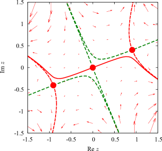
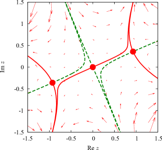
Figure 1: Changes of the Lefschetz thimbles for $\omega=1-0.9\mathrm{i}$ (left) and $\omega=1-1.1\mathrm{i}$ (right) with $\lambda=1.5\mathrm{i}$ fixed. (Left) One of three thimbles as shown by the solid line contributes to the integral and two are to be dropped when $\omega=1-0.9\mathrm{i}$. (Right) All three thimbles contribute to the integral when $\omega=1-1.1\mathrm{i}$.

When $\varepsilon$ is small enough, the Hamilton dynamics should become equivalent to the conventional formulation of the integral on the Lefschetz thimble, which means that $P(z,\bar{z})$ should have a peak along the Lefschetz thimble only. This makes the analytic treatment much accessible since we do not have to solve the quantum mechanical problem in this zero-dimensional toy model. To identify the Lefschetz thimble, we should integrate the flow equation in Eq. (3) and find the upward and the downward paths. We show the numerical results in Fig. 1 for parameters slightly changed from Eq. (15).

For our theory (14) three saddle points are located at $z_{0}=0$, $z_{\pm}=\pm\sqrt{-\omega/\lambda}$. The latter is, for our choice of parameters (15), $z_{\pm}=\pm(0.897+0.372\mathrm{i})$, and $S(z_{\pm})=-1/3$. We can see that $\omega=1-\mathrm{i}$ is a critical value at which the destinations of the downward flows from the saddle points change drastically, that is known as the Stokes phenomenon, as is clear from two panels for $\omega=1-0.9\mathrm{i}$ (left) and $\omega=1-1.1\mathrm{i}$ (right) in Fig. 1. In general we can show that the Stokes phenomenon occurs at ${\rm Im}\,(\omega^{2}/\lambda)=0$, and when $\lambda$ is pure imaginary, this condition gives ${\rm arg}\,(\omega)=-\pi/4$. Importantly, not only the downward flows but also the upward flows change and the intersection number of the original and the upward paths changes accordingly (4; 5). In the case with $\omega=1-0.9\mathrm{i}$ only one upward path from $z_{0}$ crosses the real axis as seen in the left of Fig. 1, and so the Lefschetz thimble going through $z_{0}$ contributes to the integral. In the case with $\omega=1-1.1\mathrm{i}$, on the other hand, three upward paths from $z_{0}$ and $z_{\pm}$ all cross the real axis, and all three Lefschetz thimbles contribute to the integral.

Keeping the potential application to the real-time physics in mind, we need deeper understanding on the Stokes phenomenon. In fact, it occurs at $k^{2}=m^{2}+\Gamma$ and so the thimble structure may fluctuate depending on the frequency $k^{0}$, while in Euclidean theory it never happens because $k^{2}-m^{2}$ is always negative (except for an unstable potential with $m^{2}<0$). It should be an interesting future problem to clarify the treatment of the Stokes phenomenon in the real-time systems (10).

For the same model with a different set of parameters, the Stokes phenomenon has been discussed in Refs. (27; 28) and the probability distribution $P(z,\bar{z})$ in the complex Langevin method has been numerically computed. The important insight obtained there is that $P(z,\bar{z})$ in the complex Langevin method looks localized but has a power decay at large $|z|$, which causes a convergence problem. Hence, it would be an intriguing question how $P(z,\bar{z})$ in the modified Lefschetz thimble method for $\varepsilon\neq 0$ should behave especially at large $|z|$.

4. Wave-functions at finite $\varepsilon$.

As an application of the modified Lefschetz-thimble method with a regulator $\varepsilon$, let us compute the wave-function $\Psi^{\prime}$ for the $\varepsilon=\varepsilon_{1}=\varepsilon_{2}$ case, from which $P(z,\bar{z})$ is to be constructed immediately. We can readily find the eigenstate in terms of $\psi_{i}$ for the last term in the Hamiltonian (11). By restricting ourselves to the $F=1$ sector, we can define the effective potential in a form of $2\times 2$ matrix-valued function that amounts to

$$V_{\rm eff}=\frac{1}{2\varepsilon}\biggl{[}\biggl{(}\frac{\partial{\rm Re}\,S}{\partial x_{1}}\biggr{)}^{2}+\biggl{(}\frac{\partial{\rm Re}\,S}{\partial x_{2}}\biggr{)}^{2}\biggr{]}-\biggl{(}\begin{array}[]{cc}{\partial^{2}{\rm Re}\,S/\partial x_{1}^{2}}&{\partial^{2}{\rm Re}\,S/\partial x_{1}\partial x_{2}}\\ {\partial^{2}{\rm Re}\,S/\partial x_{1}\partial x_{2}}&-{\partial^{2}{\rm Re}\,S/\partial x_{1}^{2}}\end{array}\biggr{)}\;,$$ (16)

and then the Hamiltonian is

$$H_{\rm eff}^{\prime}=-\frac{\varepsilon}{2}\biggl{(}\frac{\partial^{2}}{\partial x_{1}^{2}}+\frac{\partial^{2}}{\partial x_{2}^{2}}\biggr{)}+V_{\rm eff}\;.$$ (17)

Let us solve the ground state of the above $H_{\rm eff}^{\prime}$ at finite $\varepsilon$, and we specifically adopt $\varepsilon=1$ unless stated explicitly.

When we solve the Hamilton dynamics, we should set initial conditions to select proper Lefschetz thimbles out. We choose the semiclassical ground state in the limit $\varepsilon\to+0$ as our initial condition. Since $\Psi^{\prime}=\mathrm{e}^{\mathrm{Re}S/\varepsilon}\Psi$ and $\Psi^{(z_{\sigma})}\to\delta(\mathcal{J}_{\sigma})$ in $\varepsilon\to+0$, $\Psi^{\prime(z_{\sigma})}\sim\mathrm{e}^{\mathrm{Re}S/\varepsilon}\delta(\mathcal{J}_{\sigma})$ for small $\varepsilon$. Let us consider the Lefschetz thimble around $z_{0}$ for instance, then its tangential direction at $z_{0}$ is given by $x_{2}=\tan{(\pi/8)}x_{1}$ as seen also from Fig. 1. The initial wave-function is thus proportional to

$$\mathrm{e}^{\mathrm{Re}S(z)/\varepsilon}\delta(-\sin(\pi/8)x_{1}+\cos(\pi/8)x_{2})\cdot(-\sin(\pi/8)\mathrm{d}x_{1}+\cos(\pi/8)\mathrm{d}x_{2})\;.$$ (18)

The bosonic part is well localized at $z_{0}$, which justifies the following choice of the initial wave function, $\Psi^{\prime(z_{\sigma})}(t=-\infty)=\delta(z-z_{0})(-\sin(\pi/8)\mathrm{d}x_{1}+\cos(\pi/8)\mathrm{d}x_{2})$. Similarly, we can fix the initial wave function for $z_{\pm}$ as $\Psi^{\prime(z_{\pm})}=\delta(z-z_{\pm})(\cos(\pi/8)\mathrm{d}x_{1}+\sin(\pi/8)\mathrm{d}{x_{2}})$.

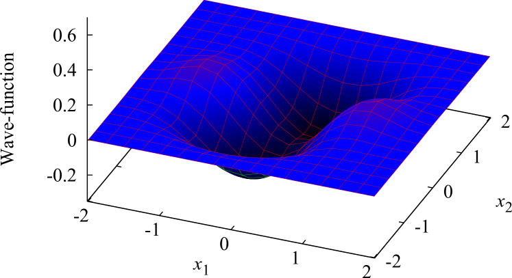
(a) $\Psi^{\prime(z_{0})}_{1}(x_{1},x_{2})$

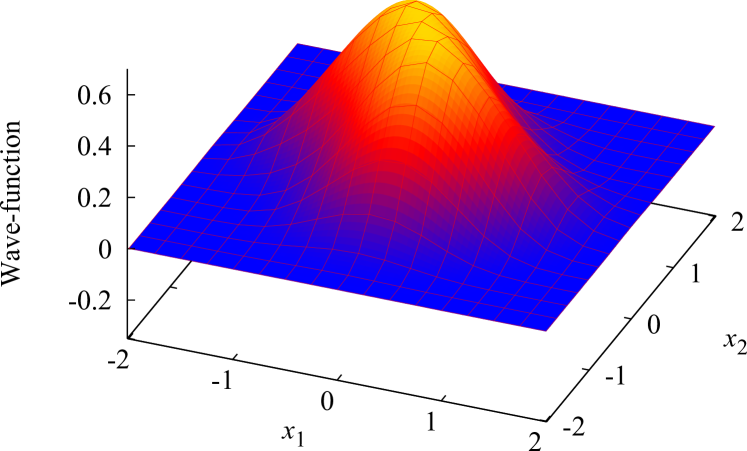
(b) $\Psi^{\prime(z_{0})}_{2}(x_{1},x_{2})$

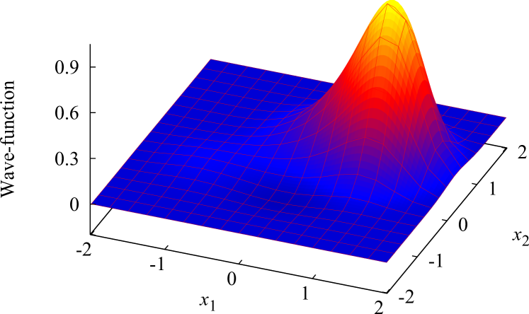
(c) $\Psi^{\prime(z_{+})}_{1}(x_{1},x_{2})$

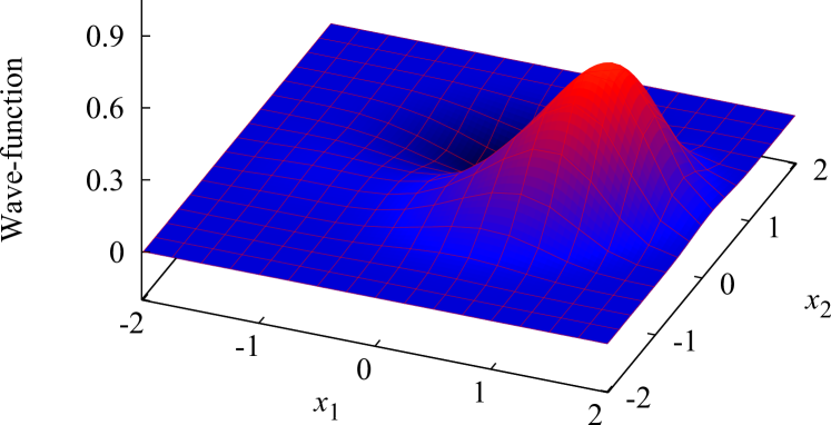
(d) $\Psi^{\prime(z_{+})}_{2}(x_{1},x_{2})$

Figure 2: SUSY ground state $\Psi^{\prime(z_{\sigma})}$ corresponding to the saddle points $z_{0}=0$ and $z_{+}=\sqrt{-\omega/\lambda}$ with $\varepsilon=1$, $\omega=1-\mathrm{i}$, and $\lambda=10^{-3}+1.5\mathrm{i}$. Denoting $\Psi^{\prime(z_{\sigma})}=\Psi^{\prime(z_{\sigma})}_{1}\mathrm{d}x_{1}+\Psi^{\prime(z_{\sigma})}_{2}\mathrm{d}x_{2}$, (a) and (b) represent $\Psi^{\prime(z_{0})}$, while (c) and (d) represent $\Psi^{\prime(z_{+})}$.

For the numerical procedure we smeared the delta function in the initial wave function by a Gaussian as $\delta(z-z_{\sigma})\to\exp\{-20[(x_{1}-x_{1\sigma})^{2}+(x_{2}-x_{2\sigma})^{2}]\}$. Then we discretized $x_{1}$ and $x_{2}$ from $-2.5$ to $+2.5$ with $\mathrm{d}x=5\times 10^{-2}$. We then numerically integrate ${\mathrm{d}\over\mathrm{d}t}{\Psi^{\prime(z_{\sigma})}}=-H_{\rm eff}^{\prime}\Psi^{\prime(z_{\sigma})}$ using the Euler method with $\mathrm{d}t=10^{-4}$ until the wave-function converges. The convergence is fast and stable and the wave-function hardly changes after $t=1\sim 2$. We also mention that we utilized the Crank-Nicolson algorithm to improve the numerical stability when we compute the Laplacian.

With this prescription, we find three independent ground state wave-functions $\Psi^{\prime(z_{\sigma})}=\Psi^{\prime(z_{\sigma})}_{1}\mathrm{d}x_{1}+\Psi^{\prime(z_{\sigma})}_{2}\mathrm{d}x_{2}$, which is shown in Fig. 2. The figures (a,b) in Fig. 2 show two components of $\Psi^{\prime(z_{0})}$ and the figures (c,d) show those of $\Psi^{\prime(z_{+})}$. Since our system is symmetric under the reflection $z\mapsto-z$, we can easily read $\Psi^{\prime(z_{-})}$ from the figures of $\Psi^{\prime(z_{+})}$. Remarkably, these ground-state wave functions are linearly independent from one another, which means that supersymmetry is unbroken. We have also verified that the Dyson–Schwinger equation,

$$\lambda\langle z^{4}\rangle+\omega\langle z^{2}\rangle=1,$$ (19)

is satisfied within $1\%$ accuracy. This clearly shows that the supersymmetric quantum mechanics provides a suitable framework to compute Lefschetz thimbles.

Let us comment on the convergence of the wave-functions in the present modified Lefschetz thimble method. In the effective potential (16), the first term gives the dominant binding potential in our toy model for large $|z|$ because the first term is a polynomial up to the sixth order, while the second term is up to the quadratic order. Therefore, the convergence in the present numerical approach is quite improved and there is no problem of the power-decay unlike the complex Langevin method. One might think that the remaining $\mathrm{e}^{\mathrm{i}{\rm Im}\,S}$ is still oscillating, but this is not a problem practically. We have numerical verified that the effect of $\mathrm{e}^{\mathrm{i}{\rm Im}\,S}$ is very small in the region where the profile of $\Psi^{\prime(z_{\sigma})}$ is localized.

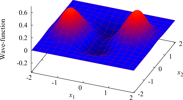
(a) $\tilde{\Psi}^{\prime(z_{0})}_{1}(x_{1},x_{2})$

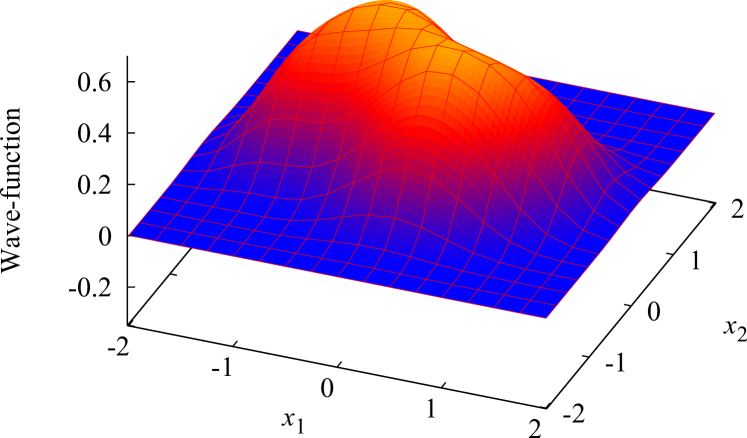
(b) $\tilde{\Psi}^{\prime(z_{0})}_{2}(x_{1},x_{2})$

Figure 3: SUSY ground state $\tilde{\Psi}^{\prime(z_{0})}$, which is obtained starting with the saddle point $z_{0}$ but with the initial relative weight equal to both components.

We also checked the robustness of the numerical results against small variations of the center position and the smearing width in initial conditions. If the smearing width of the initial wave function is changed, the overall normalization would be changed naturally, but once we normalize the wave-functions in the same manner (in Fig. 2 we normalized them as $\int\mathrm{d}x_{1}\,\mathrm{d}x_{2}[(\Psi^{\prime(z_{\sigma})}_{1})^{2}+(\Psi^{\prime(z_{\sigma})}_{2})^{2}]=1$), then we eventually get the same result. Such insensitivity implies that each wave-function is well localized and the overlap at the saddle point is small. However, the overlap at the saddle point is not completely zero. To see this effect, let us skew the relative weight of the initial condition so that the initial wave-functions are not orthogonal. In Fig. 3, we show $\tilde{\Psi}^{\prime(z_{0})}_{1}$ and $\tilde{\Psi}^{\prime(z_{0})}_{2}$ starting with the same relative weights, namely, $\tilde{\Psi}^{\prime(z_{0})}(-\infty)=\delta(z-z_{0})(\mathrm{d}x_{1}+\mathrm{d}x_{2})$ at the initial time, for the demonstration purpose. The result $\tilde{\Psi}^{\prime(z_{0})}$ in Fig. 3 is given a natural interpretation as a superposition of three ground states shown in Fig. 2. Because of this overlap among wave functions, our prescription for the initial wave function needs further refinement in order to extract one Lefschetz thimble at $\varepsilon=1$.

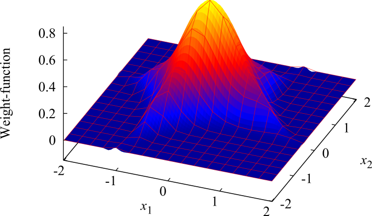
(a) $\mathrm{Re}P$ at $\omega=1-\mathrm{i}$, $\varepsilon=0.2$

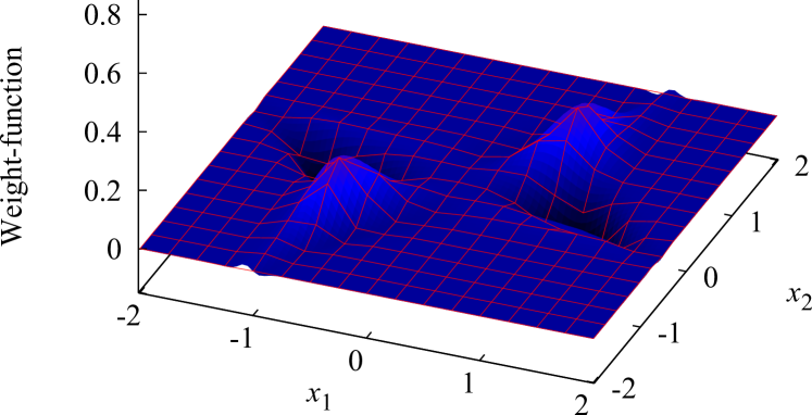
(b) $\mathrm{Im}P$ at $\omega=1-\mathrm{i}$, $\varepsilon=0.2$

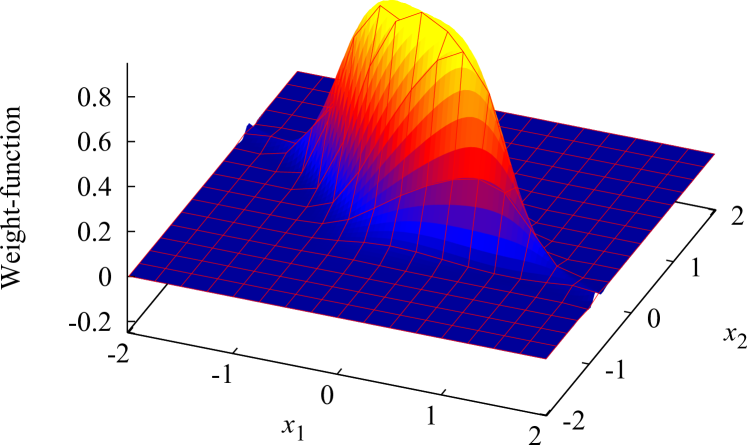
(c) $\mathrm{Re}P$ at $\omega=1+\mathrm{i}$, $\varepsilon=0.2$

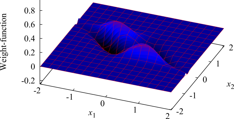
(d) $\mathrm{Im}P$ at $\omega=1+\mathrm{i}$, $\varepsilon=0.2$

Figure 4: Weight functions $P(x_{1},x_{2})$ corresponding to the saddle point $z_{0}$ with $\varepsilon=0.2$. (a) and (b) show the result for $\omega=1-\mathrm{i}$, and $\lambda=10^{-3}+1.5\mathrm{i}$. (c) and (d) show the result for $\omega=1+\mathrm{i}$, and $\lambda=10^{-3}+1.5\mathrm{i}$.

In order to see the importance of such refinements from another viewpoint, we checked behaviors of distributions $P$ for small $\varepsilon$. Let us set $\varepsilon=0.2$ with $\omega=1-\mathrm{i}$ and $\lambda=1.5\mathrm{i}$, then we obtain Figs. 4 (a) and (b). Here, the normalization is given by $\int\mathrm{d}^{2}x\,P=1$. Although it is localized around the saddle point $z_{0}=0$, its shape is still far from a one-dimensional line shown in Fig. 1. In order for comparison, we show the result also for $\varepsilon=0.2$ with $\omega=1+\mathrm{i}$ and $\lambda=1.5\mathrm{i}$ in Figs. 4 (c) and (d). For this case, $P$ is well localized to a one-dimensional line, which is nothing but the Lefschetz thimble $\mathcal{J}_{0}$ at this parameter. We numerically observed that the weight function $P$ is well localized around a Lefschetz thimble if Stokes phenomena do not happen and $\varepsilon$ is sufficiently small. Expectation values of operators, such as $\langle z^{2}\rangle$, also give correct numbers within the numerical accuracy with such parameters. However, as $\varepsilon$ becomes larger, wave functions spread as two-dimensional distributions, and expectation values of operators do not necessarily give correct values. Since the Dyson–Schwinger equation (19) is satisfied, this problem must come from superpositions of the wave function with other ground states.

It is an important future study to clarify dependence on this initial condition more systematically, in order to take an appropriate linear combination of these wave-functions giving each Lefschetz thimble. This would be a key step to study how the Stokes phenomenon is realized at $\varepsilon=1$. It also opens a new possibility to take into account multiple Lefschetz thimbles, since ground-state wave functions can be superposed by changing the initial condition.

5. Discussions and Conclusions.

In this Letter, the supersymmetric reformulation of the Lefschetz thimble integration was studied and its practical computation was discussed. The Lefschetz thimbles are now regarded as the ground sates of a supersymmetric Hamiltonian. Our computational scheme for the Hamiltonian system is essentially the same with that for the Fokker-Planck equation in the complex Langevin method. Those supersymmetric wave-functions are numerically computed for a zero-dimensional toy model with the classical action $S=S_{0}+S_{\rm int}$ where $S_{0}=-\frac{\omega}{2}x^{2}$ and $S_{\rm int}=-\frac{\lambda}{4}x^{4}$. Since the Morse indices of all the saddle points are the same, the number of saddle points must be the same as that of linearly independent ground states.

For the Gaussian model with $S_{0}$ only, the above-mentioned situation is clearly true, which is explicitly checked by computing the wave-function analytically and constructing one supersymmetric ground sate. From this almost trivial example, one can learn an important lesson about the two-dimensional smooth distribution $P_{0}(z,\bar{z})$. In the “semi-classical” limit of $\varepsilon\to 0$, we recover a delta functional support along the Lefschetz thimble in the original formulation. For non-zero $\varepsilon$, the phase oscillation arises away from the Lefschetz thimble, and the formulation nevertheless reproduces the correct expectation value.

For the interacting model with $S_{\rm int}$, we performed numerical computations for the supersymmetric quantum mechanics, and confirmed the existence of three linearly independent ground states by restricting ourselves to the $F=1$ sector. Since the wave-function in the $F=1$ sector consists of two components, we must set them in the proper initial conditions. We started from a localized wave-function in the vicinity of each saddle point, and our numerical computation shows a remarkable stability under small modifications on the initial conditions. This reflects the fact that all the saddle points are attractive unlike the complex Langevin method. At the same time we also found substantial dependence on the initial relative weight of these two components. This clearly indicates that we need a careful refinement of the initial condition to use the modified Lefschetz thimble method for numerical simulations, but it also opens a new possibility for some convenient scheme to take into account multiple Lefschetz thimbles.

In the case of the Fokker-Planck system, the ground state is often uniquely determined and the initial condition dependence does not appear as in the case in ordinary quantum mechanics without any special symmetry. The Fokker-Planck operator of the complex Langevin method can be written as a functional integral in a similar manner, and it also shows the same type of the BRST symmetry. There are, however, several important differences in these two formalisms: First of all, the diffusion term in the complex Langevin equation does not give the gradient flow because the sign is different. Because of this difference, the BRST invariance cannot be promoted to the supersymmetric system satisfying $2H=\{Q,\bar{Q}\}$ with supercharges $Q,\,\bar{Q}$. Moreover, the fermionic sector should be restricted to $F=2$ instead of $F=1$. Therefore, it is not straightforward to relate these two formalisms yet. If one could establish a firm relation between two methods, it would be a great progress and the present modified Lefschetz thimble could provide us with an opportunity for a fully complementary approach to the sign problem together with the complex Langevin method.

The authors thank Yuya Abe, So Matsuura, Jun Nishimura, and Jan Pawlowski for useful discussions. K. F. was supported by JSPS KAKENHI Grant No. 15H03652 and 15K13479. Y. T. was supported by Grants-in-Aid for JSPS fellows (No.25-6615). This work was partially supported by the RIKEN iTHES project, and also by the Program for Leading Graduate Schools, MEXT, Japan.

References

- (1) E.Y. Loh, J.E. Gubernatis, R.T. Scalettar, S.R. White, D.J. Scalapino, and R.L. Sugar, Phys.Rev., B41, 9301–9307 (1990).
- (2) Shin Muroya, Atsushi Nakamura, Chiho Nonaka, and Tetsuya Takaishi, Prog. Theor. Phys., 110, 615–668 (2003), arXiv:hep-lat/0306031.
- (3) Frédéric Pham, Vanishing homologies and the variable saddlepoint method, In Proc. Symp. Pure Math, volume 40.2, pages 319–333. AMS (1983).
- (4) Edward Witten, Analytic Continuation Of Chern-Simons Theory, In Chern-Simons Gauge Theory: 20 Years After, page 347. AMS (2010), arXiv:1001.2933.
- (5) Edward Witten (2010), arXiv:1009.6032.
- (6) Marco Cristoforetti, Francesco Di Renzo, and Luigi Scorzato, Phys.Rev., D86, 074506 (2012), arXiv:1205.3996.
- (7) Marco Cristoforetti, Francesco Di Renzo, Abhishek Mukherjee, and Luigi Scorzato, Phys.Rev., D88, 051501 (2013), arXiv:1303.7204.
- (8) H. Fujii, D. Honda, M. Kato, Y. Kikukawa, S. Komatsu, and T. Sano, JHEP, 1310, 147 (2013), arXiv:1309.4371.
- (9) M. Cristoforetti, F. Di Renzo, G. Eruzzi, A. Mukherjee, C. Schmidt, L. Scorzato, and C. Torrero, Phys.Rev., D89, 114505 (2014), arXiv:1403.5637.
- (10) Yuya Tanizaki and Takayuki Koike, Annals of Physics, 351, 250 (2014), arXiv:1406.2386.
- (11) Yuya Tanizaki, Phys. Rev., D91, 036002 (2015), arXiv:1412.1891.
- (12) Takuya Kanazawa and Yuya Tanizaki, JHEP, 1503, 044 (2015), arXiv:1412.2802.
- (13) Yuya Tanizaki, Hiromichi Nishimura, and Kouji Kashiwa, Phys. Rev., D91, 101701 (2015), arXiv:1504.02979.
- (14) Francesco Di Renzo and Giovanni Eruzzi (2015), arXiv:1507.03858.
- (15) Poul H. Damgaard and Helmuth Huffel, Phys.Rept., 152, 227 (1987).
- (16) Gert Aarts and Frank A. James, JHEP, 08, 020 (2010), arXiv:1005.3468.
- (17) Hiroki Makino, Hiroshi Suzuki, and Daisuke Takeda (2015), arXiv:1503.00417.
- (18) Jun Nishimura and Shinji Shimasaki, Phys. Rev., D92(1), 011501 (2015), arXiv:1504.08359.
- (19) J. Berges and I. O. Stamatescu, Phys. Rev. Lett., 95, 202003 (2005), arXiv:hep-lat/0508030.
- (20) J. Berges, Sz. Borsanyi, D. Sexty, and I. O. Stamatescu, Phys. Rev., D75, 045007 (2007), arXiv:hep-lat/0609058.
- (21) Ryoji Anzaki, Kenji Fukushima, Yoshimasa Hidaka, and Takashi Oka, Annals Phys., 353, 107–128 (2015), arXiv:1405.3154.
- (22) E. Frenkel, A. Losev, and N. Nekrasov, Nucl.Phys.Proc.Suppl., 171, 215–230 (2007), arXiv:hep-th/0702137.
- (23) E. Frenkel, A. Losev, and N. Nekrasov (2006), arXiv:hep-th/0610149.
- (24) E. Frenkel, A. Losev, and N. Nekrasov (2008), arXiv:0803.3302.
- (25) Edward Witten, J. Diff. Geom., 17, 661–692 (1982).
- (26) Alireza Behtash, Erich Poppitz, Tin Sulejmanpasic, and Mithat Ünsal (2015), arXiv:1507.04063.
- (27) Gert Aarts, Phys.Rev., D88, 094501 (2013), arXiv:1308.4811.
- (28) Gert Aarts, Lorenzo Bongiovanni, Erhard Seiler, and Denes Sexty, JHEP, 1410, 159 (2014), arXiv:1407.2090.