A new approach to the maser emission in the solar corona

Abstract

Aims. The electron plasma frequency $\omega_{pe}$ and electron gyrofrequency $\Omega_{e}$ are two parameters that allow us to describe the properties of a plasma and to constrain the physical phenomena at play, for instance, whether a maser instability develops. In this paper, we aim to show that the maser instability can exist in the solar corona.

Methods. We perform an in-depth analysis of the  ratio for simple theoretical and complex solar magnetic field configurations. Using the combination of force-free models for the magnetic field and hydrostatic models for the plasma properties, we determine the ratio of the plasma frequency to the gyrofrequency for electrons. For the sake of comparison, we compute the ratio for bipolar magnetic fields containing a twisted flux bundle, and for four different observed active regions. We also study how  is affected by the potential and non-linear force-free field models.

Results. We demonstrate that the ratio of the plasma frequency to the gyrofrequency for electrons can be estimated by this novel method combining magnetic field extrapolation techniques and hydrodynamic models. Even if statistically not significant, values of  $\leq$ 1 are present in all examples, and are located in the low corona near to photosphere below one pressure scale-height and/or in the vicinity of twisted flux bundles. The values of   are lower for non-linear force-free fields than potential fields, thus increasing the possibility of maser instability in the corona.

Conclusions. From this new approach for estimating , we conclude that the electron maser instability can exist in the solar corona above active regions. The importance of the maser instability in coronal active regions depends on the complexity and topology of the magnetic field configurations.

1 Introduction

Loss-cone driven instabilities play an important role in space plasmas. The emission of non-thermal radiation is still a puzzling process despite the accurate observations made in other fields, such as planetary magnetospheres (Treumann, 2006). This emission is often explained by the cyclotron maser mechanism for which the $X$-mode and its harmonics provide the escaping radiation. The growth rate of the $X$-modes depends on the value of the ratio of the electron plasma frequency to the electron gyrofrequency (hereafter $\Xi_{e}$). Sharma & Vlahos (1984) studied the development of the $X$-modes and $O$-modes under the physical conditions of plasmas in the low corona. The study has been performed for values of $\Xi_{e}$ less than 2.5. The authors showed that (i) the electron maser instability dominates the emission for $\Xi_{e}\leq 1$ over other loss-cone driven instabilities, and (ii) the first harmonic of the $X$-mode dominates for $\Xi_{e}<0.35$. In solar physics, the electron maser instability has been studied to explain the spiky radio burst observed during flares (Holman et al., 1980; Melrose & Dulk, 1982). Similar studies have revealed the importance of the $\Xi_{e}$ thresholds at 0.35 and 1 for the growth of $X$-modes (e.g. Melrose et al., 1984; Winglee, 1985; Vocks & Mann, 2004; Tang & Wu, 2009; Lee et al., 2013). The question arising from these studies is, Can electron cyclotron maser emission be a viable mechanism in the solar corona? To tackle this question, we estimate the ratio $\Xi_{e}$ in the low corona by assuming that the corona is in equilibrium and thus can be described by a force-free equilibrium for the magnetic field and a hydrostatic equilibrium for the plasma parameters.

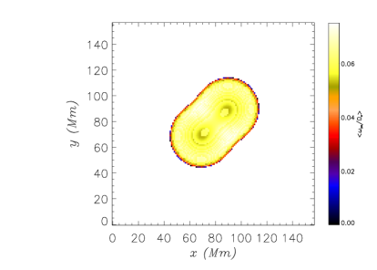
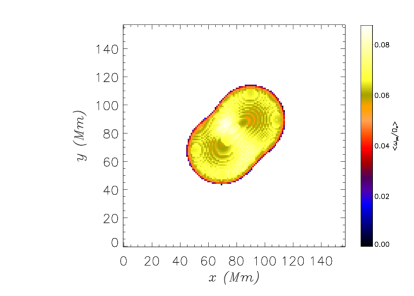
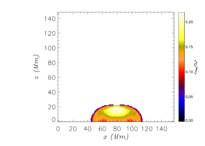
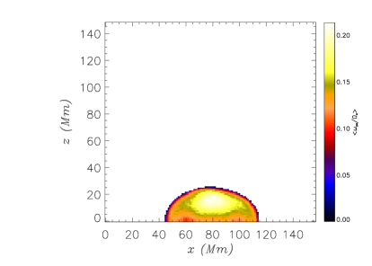
Figure 1: Spatial distribution of $\Xi_{e}\leq 1$ for the bipolar field. (top row) top view; (bottom row) side view for the potential (left) and nlff (right) magnetic fields with varying gravity. The values of $\Xi_{e}$ are averaged along the 3rd dimension. Only the $\Xi_{e}\leq 1$ values are colour-coded.

The electron population of a plasma can be described by two characteristic frequencies amongst other parameters: the electron plasma frequency, $\omega_{pe}$, and the electron gyrofrequency, $\Omega_{e}$. The plasma frequency of a cold plasma (neglecting the thermal velocity) is given by

$$\omega_{pe}=\sqrt{\frac{n_{e}e^{2}}{m_{e}\epsilon_{0}}},$$ (1)

where $n_{e}$ is the electron number density, $e$ is the electric charge (1.6022$\times$10^-19 C), $m_{e}$ is the electron mass (9.1094$\times$10^-31 kg), and $\epsilon_{0}$ is the permittivity of free space (8.8542$\times$10^-12 F m^-1). The gyrofrequency of electrons is given by

$$\Omega_{e}=\frac{eB}{m_{e}},$$ (2)

where $B$ is the magnetic field strength. The ratio of the two frequencies, $\Xi_{e}=\omega_{pe}/\Omega_{e}$, can thus be expressed as the ratio of the speed of light to the Alfvén speed,

$$\Xi_{e}=\frac{1}{1.14R}\frac{c}{v_{A}},$$ (3)

where $R$ is the mass ratio between protons and electrons ($R=1836$) and the coefficient $1.14$ is obtained for a coronal plasma with a mean atomic weight of $\tilde{\mu}=0.6$. Thus, knowing the Alfvén speed from the low-order magnetohydrostatic model developed by Régnier et al. (2008), we derive $\Xi_{e}$ for different magnetic field configurations. This new method is then used to determine whether the maser instability is a viable mechanism in the solar corona.

The paper is organised as follows: after summarising the magnetic field and hydrostatic models in Section 2, we present the estimate of  for a simple bipolar configuration in Section 3, and for four different active regions in Section 4. We summarise our findings and conclude in Section 5.

2 Magnetic field and density models for the solar corona

As in Régnier et al. (2008), we combine two models to describe the properties of magnetised plasma in the solar corona: the coronal magnetic field is assumed to be a force-free field, and the plasma properties are derived from a stratified atmosphere in hydrostatic equilibrium. In the following sections, we briefly summarise the different numerical models.

2.1 Potential and non-linear force-free models

Magnetic field extrapolations are well-known techniques for describing the 3D nature of the coronal magnetic fields (see review by Régnier, 2013). Under coronal conditions, the magnetic forces dominate the pressure gradient and gravity, and so we regard the corona above active regions as being well described by the force-free approximation (see e.g. recent reviews by Wiegelmann & Sakurai, 2012; Régnier, 2013, and references therein). Throughout this article, the coronal magnetic configurations are computed from the non-linear force-free (nlff) approximation based on a vector potential Grad-Rubin (1958) method by using the XTRAPOL code (Amari et al., 1997, 1999). The nlff field is governed by the following equations,

$$\@vec{\nabla}\times\@vec{B}=\alpha\@vec{B},$$ (4)

$$\@vec{B}\cdot\@vec{\nabla}\alpha=0,$$ (5)

$$\@vec{\nabla}\cdot\@vec{B}=0,$$ (6)

where $\@vec{B}$ is the magnetic field vector in the domain $\Omega$ above the photosphere, $\delta\Omega$; $\alpha$ is a function of space defined in Cartesian coordinates as the ratio of the vertical current density, $J_{z}$; and the vertical magnetic field component, $B_{z}$:

$$\alpha=\frac{1}{B_{z}}\leavevmode\nobreak\ \left(\frac{\partial B_{y}}{\partial x}-\frac{\partial B_{x}}{\partial y}\right).$$ (7)

From Eq. (5), $\alpha$ is constant along a field line, but varies across field lines. The full description of the Grad-Rubin iterative scheme can be found in Amari et al. (1997), and the vector magnetograms used as boundary conditions for the following examples have been detailed, for instance, in Régnier et al. (2008).

For the sake of comparison, we compute both the potential and nlff fields following the technique developed by Grad & Rubin (1958).

2.2 Hydrostatic model

In order to define the thermodynamics parameters of the coronal plasma, we assume that the corona is an isothermal atmosphere satisfying the hydrostatic equilibrium

$$-\@vec{\nabla}p+\rho\@vec{g}=\@vec{0},$$ (8)

where $p$ is the plasma pressure, $\rho$ is the density, and $\@vec{g}$ is the gravitational force. In agreement with the Harvard-Smithonian model of the solar atmosphere, we consider the hydrostatic equilibrium to be a reasonable assumption above the photosphere at a height ($z_{0}$) of about 5 Mm. As shown in Régnier et al. (2008), it is more appropriate to consider the variation with height of the gravitational field in order to satisfy the continuity with the properties of the solar wind. Therefore, we will only consider the case of varying gravity satisfying the following equations for the plasma pressure and density,

$$\centering\left\{\begin{array}[]{c l}p(z)=p_{0}\exp{\left(-\frac{R_{\odot}^{2}}{H\leavevmode\nobreak\ (R_{\odot}+z_{0})}\left(\frac{z-z_{0}}{R_{\odot}+z}\right)\right)},&\quad\textrm{and}\\[5.69046pt] \rho(z)=\rho_{0}\exp{\left(-\frac{R_{\odot}^{2}}{H\leavevmode\nobreak\ (R_{\odot}+z_{0})}\left(\frac{z-z_{0}}{R_{\odot}+z}\right)\right)}&\quad\textrm{for $g=g(z)=\frac{g_{0}\leavevmode\nobreak\ R_{\odot}^{2}}{(R_{\odot}+z)^{2}}$,}\\ \end{array}\right.\@add@centering$$ (9)

where $H=k_{B}T/(\tilde{\mu}m_{p}g_{0})$ is the pressure scale-height ($k_{B}=1.38\leavevmode\nobreak\ 10^{-23}$ J K^-1, $\tilde{\mu}=0.6$ for a fully ionised coronal plasma, $m_{p}=1.67\leavevmode\nobreak\ 10^{-27}$ kg, and $g_{0}=g(R_{\odot})=274$ m s^-2), and $p_{0}$ and $\rho_{0}$ are characteristic values of the plasma pressure and density at $z_{0}$. The pressure scale-height and the density $\rho_{0}$ are the two free parameters of the model. Typical values are $H=50$ Mm giving a coronal temperature of 1 MK and the number density correpsonding to $\rho_{0}$ is $n_{0}=10^{9}$ cm^-3.

For a gravitational field varying with height, the Alfvén speed is thus given by

$$v_{A}(x,y,z)=\frac{B(x,y,z)}{\sqrt{\mu_{0}\rho_{0}}}\exp{\left(\frac{R_{\odot}^{2}}{2H\leavevmode\nobreak\ (R_{\odot}+z_{0})}\left(\frac{z-z_{0}}{R_{\odot}+z}\right)\right)},$$ (10)

where $B$ is the magnetic field strength.

Figure 2: Distribution of $\Xi_{e}$ for the bipolar magnetic field within the entire computational volume (cutoff at $\Xi_{e}=30$) for the potential (dashed line) and nlff (solid line) magnetic field models. The vertical dashed black line is the $\Xi_{e}=1$ threshold.

In summary, for all cases (bipolar field, and active regions), we use two different models (potential field and nlff field both with a varying gravity) to analyse the variation of the  ratio.

3 Bipolar fields

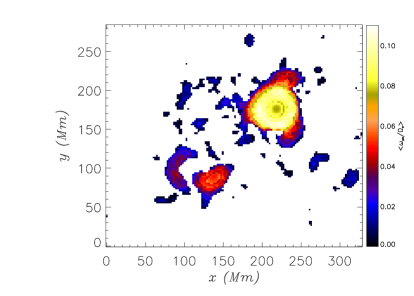
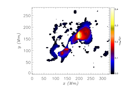
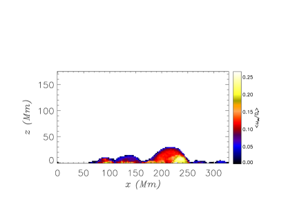
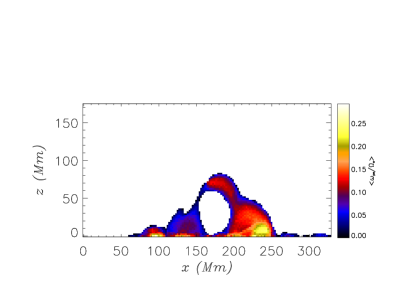
Figure 3: Same as Fig. 1 for AR8151

As a test case for the above method, we use a simple bipolar magnetic field distribution on the photosphere. For all models, the vertical component of the magnetic field, $B_{z}$, is given by a Gaussian distribution. To compute the nlff field, the vertical electric current density is injected in the magnetic configuration following a photospheric distribution of the form

$$J_{z}(r)=2\leavevmode\nobreak\ J_{z0}\leavevmode\nobreak\ [r^{2}-C_{0}]\leavevmode\nobreak\ \exp{\left(-\frac{r^{2}}{\sigma^{2}}\right)},$$ (11)

where $r$ is measured from the centre of the magnetic polarity and $C_{0}$ is a constant that ensures a zero net current. This $J_{z}$ distribution is typically a second-order Hermite polynomial function that allows for return current on the surface of the flux tube (see Régnier 2012). The vertical magnetic field strength $B_{z}$ is 2000 G at the centre of the polarities and $J_{z}$ has a maximum strength of 10 mA m^-2. Both the potential and nlff models are computed on a 148$\times$148$\times$148 computational box with a pixel size of 1 Mm.

In Fig. 1, we plot the spatial distribution of $\Xi_{e}\leq 1$ for the potential and nlff fields with varying gravity (from left to right). The first row shows a top view ($xy$-plane), whilst the second row shows a side view ($xz$-plane). The values of $\Xi_{e}$ are averaged along the third dimension. The values of $\Xi_{e}\leq 1$ are localised where the magnetic field strength is strong, below a height of 25 Mm. For this bipolar magnetic field configuration, the values of $\Xi_{e}$ are similar across both models (see also Table 1).

The distributions of $\Xi_{e}$ within the volume are shown for both models in Fig. 2 (values of $\Xi_{e}$ between 0 and 30). The two distributions have similar shapes with two main peaks around 10 and 15, and a tail for large values of $\Xi_{e}$ which tends to zero. For $\Xi_{e}\leq 1$, the distributions have a number of occurrences which is not significant whatever the magnetic field model. We confirm this in Table 1 by listing the percentage of $\Xi_{e}$ in given intervals. We use the same intervals as in Sharma & Vlahos (1984). The percentage of $\Xi_{e}\leq 1$ is about 1.5% for all models, whilst $\sim$95% of $\Xi_{e}$ values are above 2.5. In this example, the models with varying gravity give similar results whether or not the magnetic configuration contains electric currents. Thus, the maser emission is weakly influenced by the electric currents or the twist and shear in a simple magnetic configuration (without a topology).

The conclusions from this test case are (i) values of $\Xi_{e}\leq 1$ exist in coronal-like magnetic field configurations, and (ii) these values are located above large photospheric magnetic field strengths.

4 Active regions

We now analyse the values of  for four active regions at different stages of their evolution.

AR8151

Figure 4: Same as Fig. 2 for (a) AR8151, (b) AR8210, (c) AR9077, and (d) AR10486

The active region AR8151 is an old decaying active region with moderate and highly twisted flux bundles observed as a filament and an X-ray sigmoid, respectively (Régnier et al., 2002; Régnier & Amari, 2004). In Fig. 3, the $\Xi_{e}\leq 1$ values are located where the magnetic field strength is large, i.e. above sunspots and plages. For the potential model, the values of $\Xi_{e}\leq 1$ are concentrated below 30 Mm, i.e. within one pressure scale-height above the surface. For the nlff model, the spatial distribution shows significant values of $\Xi_{e}$ above 50 Mm; these values characterise the influence of electric currents present in the magnetic configuration and are associated with highly twisted flux bundles and sheared arcades. The twisted flux bundles existing in this active region generate a local increase in the magnetic field strength, i.e. in the local Alfvén speed (see Eq. 10). As can be seen in Fig. 4a, the distribution of $\Xi_{e}$ peaks at 2 for the nlff model and at 5 for the potential model. Both distributions are narrower (with a typical width of about 2) than in the magnetic bipole example presented in Section 3. Unlike the bipolar field, there is a clear difference between the potential and nlff models; the $\Xi_{e}$ values are smaller for the nlff magnetic field. Both distributions have a tail that becomes statistically insignificant for values of  above 10. These results lead us to consider that, for this active region, the nlff model has a different behaviour than the potential field model owing to the presence of twisted flux bundles and the complexity of the magnetic field; a proxy of the complexity of the coronal magnetic field is given by the complexity of the photospheric magnetic field. In terms of statistics, Table 1 shows that values of $\Xi_{e}\leq 1$ represent $\sim$0.8% for the potential model and $\sim$1.4% for the nlff model. The main difference is in the percentage of $\Xi_{e}$ between 1 and 2.5, which reaches 40% for the nlff field, whilst it is just around 8% for the potential model; as noticed previously, this is due to the strong electric currents present in the active region, which imply sheared and twisted magnetic field lines leading to the conclusion that more realistic magnetic fields like the nlff model are more favourable to maser emission.

AR8210

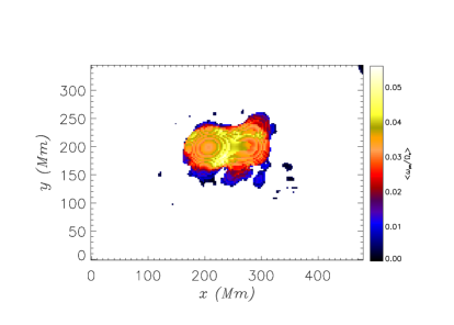
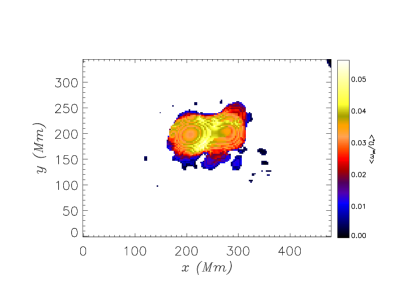
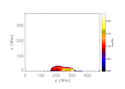
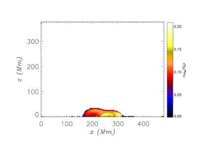
Figure 5: Same as Fig. 1 for AR8210

AR8210 is a relatively new active region which has produced numerous flares. The main features in AR8210 are a clockwise-rotating sunspot surrounded by diffuse polarities of opposite sign, and a small emerging parasitic polarity interacting with the pre-existing magnetic topology of the field (Régnier & Canfield, 2006). A time series of nlff magnetic field extrapolations has shown that the 3D magnetic configuration is close to potential (no twisted bundles, and small noticeable sheared arcades) and does not contain a large amount of free magnetic energy (estimated to $\Delta E_{m}=2.6\leavevmode\nobreak\ 10^{31}$ erg), i.e. not sufficient to produce large flares.

In Fig. 5, we plot the spatial distribution of $\Xi_{e}$ within the whole computational volume. As for the bipolar field described in Section 3, the values of $\Xi_{e}\leq 1$ are located just above the strong magnetic field regions and do not extend above 30 Mm. In Fig. 4b, the distributions of $\Xi_{e}$ indicate that the significant values of the ratio are above 3. As noted for AR8151, the nlff model decreases significantly the values of $\Xi_{e}$ compared to the potential field model. The $\Xi_{e}$ distribution peaks between 7 and 13 for the nlff model, whilst it peaks at 27 for the potential model. In terms of statistics (see Table 1), the percentage of $\Xi_{e}\leq 1$ is less than 0.5% for both models, and the percentage of $\Xi_{e}\geq 2.5$ is about 98%. These results are consistent with the fact that no twisted flux bundles or highly sheared arcades have been found in the 3D extrapolated magnetic field (Régnier & Canfield, 2006).

AR9077

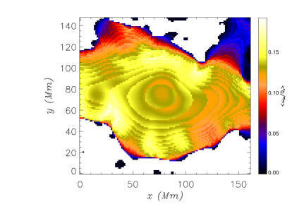
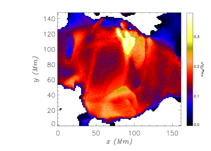
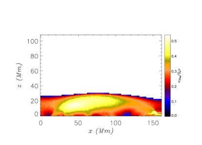
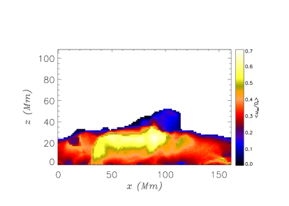
Figure 6: Same as Fig. 1 for AR9077

AR9077 produced a X5.7 flare on 2000 July 14 known as the Bastille Day flare (e.g. Kosovichev & Zharkova, 2001; Wang et al., 2005). The magnetic field extrapolation was performed after the occurrence of the X-class flare and thus describes the relaxation phase associated with post-flare loops. It has been shown that the magnetic field configuration is quite close to a potential field with a small amount of shear and twist. These magnetic field properties are reflected in the spatial distribution of $\Xi_{e}$ (Fig. 6): the $\Xi_{e}\leq 1$ values are concentrated above regions of large magnetic field strengths as was seen for the previous examples. Both potential and nlff fields have similar spatial distributions below 30 Mm. Futhermore, the nlff field exhibits an excess of low $\Xi_{e}$ values above 30 Mm indicating the presence of twisted/sheared magnetic field lines increasing locally the magnetic field strength. Compared to AR8151 (see Fig. 3), the volume containing the $\Xi_{e}\leq 1$ values above 30 Mm is small, and does indicate a small amount of twist or shear in the magnetic configuration. In Fig. 4c, the distributions for both models peak at about 1 with a percentage of values with $\Xi_{e}\leq 1$ between 14% and 19% (see Table 1). It reinforces the fact that the magnetic configuration of AR9077 at this stage of its evolution is close to potential, although the number of locations where the maser instability could occur is large (about 20%), filling the volume below 30 Mm almost entirely.

AR10486

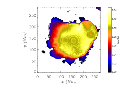
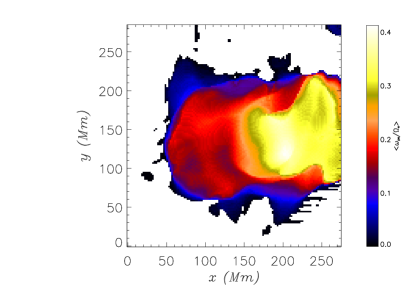
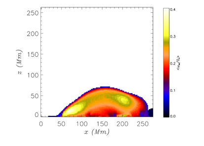
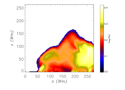
Figure 7: Same as Fig. 1 for AR10486

The active region AR10486 is the source of the series of strong flares in October-November 2003 known as the Halloween events, including the strongest flare recorded for the corresponding solar cycle estimated to be a X28 flare on November 4. The magnetic field configuration presented here is obtained before the occurrence of the X17 flare located near the disk centre on October 28. For this flare, the energetics and magnetic topology have been studied in detail (see e.g. Régnier et al., 2005; Mandrini et al., 2006; Zuccarello et al., 2009); the magnetic energy contained in this active region has been estimated to be above 10³³ erg, consistent with a large total photospheric magnetic flux. For the potential model (see Fig. 7), the $\Xi_{e}\leq 1$ values are located above strong photospheric magnetic field strength and extend in a volume below 70 Mm. For the nlff field, the model generates low $\Xi_{e}$ values high in the corona up to 170 Mm. These high-altitude, low values of $\Xi_{e}$ correspond to several pressure scale-heights. This indicates that not only is the pressure scale-height important for this model (as noted for the previous active regions), but also that the magnetic scale-height is relevant when the total unsigned magnetic flux on the photosphere is large. In Fig. 4d, all the distributions of $\Xi_{e}$ peak at 1; however, the nlff distribution has a larger number of occurrences and a narrower width, with 80% of the values being between 0 and 2.5, compared to the potential distribution which has an extended tail towards large values of $\Xi_{e}$. This is reflected in Table 1, which shows that the nlff magnetic configuration produces a larger number of favourable locations for maser emission in the corona.

5 Conclusions

Table 1: Percentage of pixels within the computational domain having a $\Xi_{e}$ included in the given range for the five different examples and for both potential and nlff magnetic field models with varying gravity.

	Model	$\Xi_{e}\leq 0.35$	$0.35<\Xi_{e}\leq 1$	$1<\Xi_{e}\leq 2.5$	$\Xi_{e}>2.5$
Bipole	Potential	0.41%	1.09%	2.76%	95.74%
	nlff	0.43%	1.18%	3.06%	95.33%
AR8151	Potential	0.05%	0.73%	7.83%	91.39%
	nlff	0.05%	1.33%	39.93%	58.69%
AR8210	Potential	0.10%	0.37%	0.88%	98.65%
	nlff	0.10%	0.37%	0.93%	98.60%
AR9077	Potential	2.50%	11.48%	34.64%	51.38%
	nlff	2.99%	15.53%	39.28%	42.20%
AR10486	Potential	1.74%	4.89%	14.06%	79.31%
	nlff	2.48%	12.13%	48.83%	36.56%

Using a combination of force-free extrapolation and hydrostatic models, we estimate the  ratio of coronal magnetic configurations above active regions. The  ratio is important in order to determine in which regime the plasma can evolve and what kind of electronic plasma waves can propagate and grow. The main electronic wave modes are the $O$- and $X$-type for the maser emission, the whistler mode, and the upper hybrid mode (electrostatic mode). The different regimes in which these modes grow or are suppressed is essentially a function of the  ratio. Melrose & Dulk (1982) have mentioned that the growth of the first and second harmonics of the $X$-mode may be responsible for observed radio and hard X-ray emission in the solar corona. The study of Sharma & Vlahos (1984) has defined intervals of  in which the different modes are important. For instance, the first harmonic of the $X$-mode has a maximum growth rate for $\leq$ 0.35, whilst the first harmonic of the $O$-mode dominates when 0.35$\leq$  $\leq$ 1. The second harmonic of the $X$-mode is dominant for 1$\leq$  $\leq$ 1.45. These values are obtained in the case where the coupling with other wave modes is neglected. Therefore, it is important to know what values of  can be expected in a realistic magnetic field above active regions and thus to check if the electron-cyclotron maser emission can be a viable mechanism in the solar corona. To achieve these goals, we develop a zero-order magnetohydrostatic model that neglects the coupling between the magnetic field and the plasma (Régnier et al., 2008). Applying this method to several active regions, we found that  can be less than 0.35 in both potential and nlff field models; however, this is statistically marginal and thus localised in small coronal volumes.

The two main results obtained from this study are:

• The smallest values of  are located where the magnetic field strength is the largest at the bottom of the corona over sunspots; this is true whatever the magnetic field model used.

• Values of  less than 1 can be found high in the corona in the case where highly twisted flux tubes can be found within the magnetic configuration; this is only obtained in magnetic field models containing electric currents.

From this new technique for estimating  in coronal plasmas, we conclude that the maser instability/emission is a viable mechanism. As mentioned by Melrose & Dulk (1982), the second harmonics of the $O$- and $X$-modes are the most possible modes to be observed, whilst the possibility of observing the first harmonic of the $X$-mode is statistically insignificant. In addition, the possible emission is most likely to be localised at the bottom of the corona or at coronal heights where the free magnetic energy is locally increased (for instance, near twisted flux bundles). We also note that both the pressure and magnetic field scale-heights are important in order to describe the variation of the Alfvén speed and thus the distribution of .

The low values of  localised high in the corona (see Fig. 3 and Fig. 7) are situated above twisted flux bundles for AR8151 and above sheared arcades for AR10846, and are indeed related to the complex magnetic topology of the fields induced by those structures. To understand better the role that these low  values play in the activity of an active region, the next step is to follow the time evolution of an active region producing observed radio emission consistent with the maser instability.

Appendix A Maser emission and twisted flux tubes in a constant gravity field

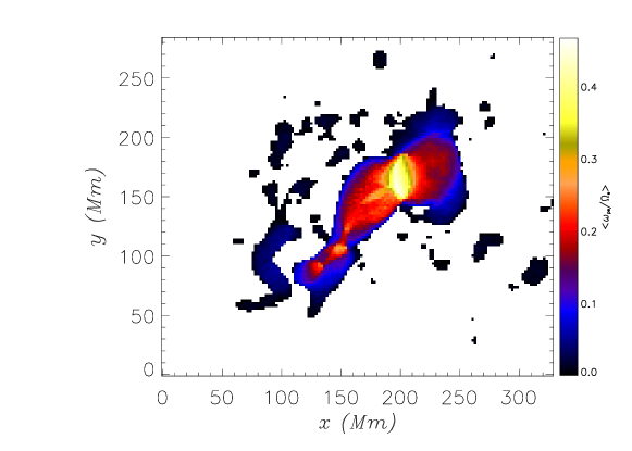
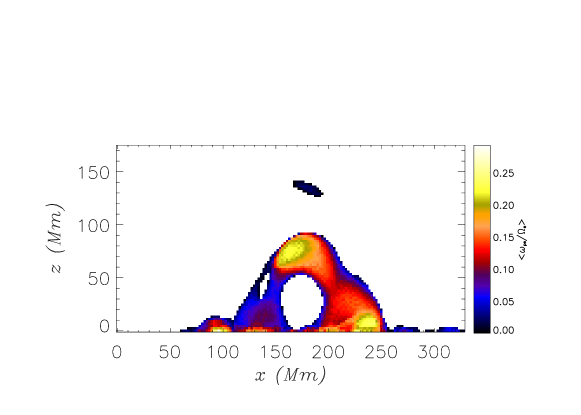
Figure 8: Same as Fig. 1 for AR8210

For the sake of completeness, we present the $\Xi_{e}$ values derived for AR8151 in the case of a nlff field with constant gravity, which exhibits a peculiar feature. For the constant gravity model, the plasma pressure and density, and the Alfvén speed are thus given by

$$\centering\left\{\begin{array}[]{c l}p(z)=p_{0}\exp{\left(-\frac{z-z_{0}}{H}\right)},&\quad\textrm{and}\\[5.69046pt] \rho(z)=\rho_{0}\exp{\left(-\frac{z-z_{0}}{H}\right)}&\quad\textrm{for $g=g_{0}$}\\ \end{array}\right.\@add@centering$$ (12)

and

$$v_{A}(x,y,z)=\frac{B(x,y,z)}{\sqrt{\mu_{0}\rho_{0}}}\exp{\left(\frac{z-z_{0}}{2H}\right)},$$ (13)

where $H=k_{B}T/(\tilde{\mu}m_{p}g_{0})$ is the pressure scale-height ($k_{B}=1.38\leavevmode\nobreak\ 10^{-23}$ J K^-1, $\tilde{\mu}=0.6$ for a fully ionised coronal plasma, $m_{p}=1.67\leavevmode\nobreak\ 10^{-27}$ kg, and $g_{0}=274$ m s^-2), and $p_{0}$ and $\rho_{0}$ are characteristic values of the plasma pressure and density at $z_{0}$. In Fig. 8, an isolated blob of low $\Xi_{e}$ values appears at a height of about 130 Mm. Comparing with Fig. 5, the blob is not present in the nlff model with varying gravity. The blob is located above the highly twisted flux tube that has been defined in Régnier & Amari (2004). A possible explanation for the appearance of the blob in this particular model is that the existence of the twisted flux tube changes the decay rate of the magnetic field strength (i.e. the magnetic field scale-height), whilst the density still follows the hydrostatic decay with height. The blob does not appear when the gravity varies with height because the density drops faster than the magnetic field strength as emphasised in Fig. 7 of Régnier et al. (2008). The blob is thus an artefact of this particular model; however, its existence emphasises the importance of understanding the variation of both the magnetic and pressure scale-heights within the corona.