Bounded Perturbation Resilience of Projected Scaled Gradient Methods

Abstract

We investigate projected scaled gradient (PSG) methods for convex minimization problems. These methods perform a descent step along a diagonally scaled gradient direction followed by a feasibility regaining step via orthogonal projection onto the constraint set. This constitutes a generalized algorithmic structure that encompasses as special cases the gradient projection method, the projected Newton method, the projected Landweber-type methods and the generalized Expectation-Maximization (EM)-type methods. We prove the convergence of the PSG methods in the presence of bounded perturbations. This resilience to bounded perturbations is relevant to the ability to apply the recently developed superiorization methodology to PSG methods, in particular to the EM algorithm.

1 Introduction

In this paper we consider convex minimization problems of the form

$$\left\{\begin{array}[c]{ll}\operatorname*{minimize}&\displaystyle J(x)\\ \text{subject to}&\displaystyle x\in\Omega.\end{array}\right.$$ (1)

The constraint set $\Omega\subseteq\mathbb{R}^{n}$ is assumed to be nonempty, closed and convex, and the objective function $J:\Omega\mapsto\mathbb{R}$ is convex. Many problems in engineering and technology can be modeled by (1). Gradient-type iterative methods are advocated techniques for such problems and there exists an extensive literature regarding projected gradient or subgradient methods as well as their incremental variants, see, e.g., Bertsekas1999Nonlinear ; HelouNeto2009Incremental ; Kiwiel2004Convergence ; Nesterov2004Introductory ; Polyak1987Introduction .

In particular, the weighted Least-Squares (LS) and the Kullback-Leibler (KL) distance (also known as I-divergence or cross-entropy Csiszar1991Why ), which are two special instances of the Bregman distances (Censor1997Parallel, , p. 33), are generally adopted as proximity functions measuring the constraints-compatibility in the field of image reconstruction from projections Byrne2001Proximity ; Byrne1993Iterative ; Combettes1994Inconsistent ; Jiang2001Development . Minimization of the LS or the KL distance with additional constraints, such as nonnegativity, naturally falls within the scope of (1). Correspondingly, the Landweber iteration Landweber1951iteration is a general gradient method for weighted LS problems (Bertero1998Introduction, , Section 6.2), (Cegielski2013Iterative, , Section 4.6), Jiang2003Convergence , McCormick1975uniform , Piana1997Projected , while the class of expectation-maximization (EM) algorithms Shepp1982Maximum are essentially scaled gradient methods for the minimization of KL distance Bertero2008Iterative ; HelouNeto2005Convergence ; Lanteri2001general .

Motivated by the scaled gradient formulation of EM-type algorithms, we focus our attention on the family of projected scaled gradient (PSG) methods, the basic iterative step of which is given by

$$x^{k+1}:=P_{\Omega}(x^{k}-\tau_{k}D(x^{k})\nabla J(x^{k})),$$ (2)

where $\tau_{k}$ denotes the stepsize, $D(x^{k})$ is a diagonal scaling matrix and $P_{\Omega}$ is the orthogonal (Euclidean least distance) projection onto $\Omega$. To our knowledge, the PSG methods presented here date back to (Bertsekas1976Goldstein, , Eq. (29)) and they resemble the projected Newton method studied in Bertsekas1982Projected .

From the algorithmic structural point of view, the family of PSG methods includes, but is not limited to, the Goldstein-Levitin-Polyak gradient projection method Bertsekas1976Goldstein ; Goldstein1964Convex ; Levitin1966Constrained , the projected Newton method Bertsekas1982Projected , and the projected Landweber method (Bertero1998Introduction, , Section 6.2), Piana1997Projected , as well as generalized EM-type methods HelouNeto2005Convergence ; Lanteri2001general . The PSG methods should be distinguished from the scaled gradient projection (SGP) methods in the literature Bertero2008Iterative ; Bonettini2009scaled . PSG methods belong to the class of two-metric projection methods Gafni1984Two , which adopt different norms for the computation of the descent direction and the projection operation while SGP methods utilize the same norm for both.

The main purpose of this paper is to investigate the convergence behavior of PSG methods and their bounded perturbation resilience. This is inspired by the recently developed superiorization methodology (SM) Censor2010Perturbation ; Censor2013Projected ; Herman2012Superiorization . The superiorization methodology works by taking an iterative algorithm, investigating its perturbation resilience, and then, using proactively such permitted perturbations, forcing the perturbed algorithm to do something useful in addition to what it is originally designed to do. The original unperturbed algorithm is called the “Basic Algorithm” and the perturbed algorithm is called the “Superiorized Version of the Basic Algorithm”.

If the original algorithm is computationally efficient and useful in terms of the application at hand, and if the perturbations are simple and not expensive to calculate, then the advantage of this methodology is that, for essentially the same computational cost of the original Basic Algorithm, we are able to get something more by steering its iterates according to the perturbations.

This is a very general principle, which has been successfully used in some important practical applications and awaits to be implemented and tested in additional fields; see, e.g., the recent papers rand-conmath ; sh14 , for applications in intensity-modulated radiation therapy and in nondestructive testing. The principles of superiorization and perturbation resilience along with many references to works in which they were used, are reviewed in the recent censor-weak-14 and gth-sup4IA . A chronologically ordered bibliography of scientific publications on the superiorization methodology and perturbation resilience of algorithms has recently been compiled and is being continuously updated by the second author. It is now available at: http://math.haifa.ac.il/yair/bib-superiorization-censor.html.

In a nutshell, the SM lies between feasibility-seeking and constrained minimization. It is not quite trying to solve the full-fledged constrained minimization; rather, the task is to seek a superior feasible solution in terms of the given objective function. This can be beneficial for cases when an exact approach to constrained minimization has not yet been discovered, or when exact approaches are computer resources demanding or computation time consuming. In such cases, existing feasibility-seeking algorithms that are perturbation resilient can be turned into efficient algorithms that perform superiorization.

The basic idea of the SM originates from the discovery that some feasibility-seeking projection algorithms for convex feasibility problems are bounded perturbations resilient Butnariu2007Stable . SM thus takes advantage of the perturbation resilience property of the String-Averaging Projections (SAP) Censor2012Convergence or Block-Iterative Projections (BIP) Davidi2009Perturbation ; Nikazad2012Accelerated methods to steer the iterates of the original feasibility-seeking projection method towards a reduced, but not necessarily minimal, value of the given objective function of the constrained minimization problem at hand, see, e.g., Censor2010Perturbation ; Penfold2010Total .

The mathematical principles of the SM over general consistent “problem structures” with the notion of bounded perturbation resilience were formulated in Censor2010Perturbation . The framework of the SM was extended to the inconsistent case by using the notion of strong perturbation resilience Herman2012Superiorization . Most recently, the effectiveness of the SM was demonstrated by a performance comparison with the projected subgradient method for constrained minimization problems Censor2013Projected .

But the SM is not limited to handling just feasibility-seeking algorithms. It can take any “Basic Algorithm” that is bounded perturbations resilient and introduce certain permitted perturbations into its iterates, such that the resulting algorithm is automatically steered to produce an output that is superior with respect to the given objective function. See Subsection 4.1 below for more details on this point.

Specifically, efforts have been recently made to derive a superiorized version of the EM algorithm, and this is why we study the bounded perturbation resilience of the PSG methods here. Superiorization of the EM algorithm was first reported experimentally in our previous work with application to bioluminescence tomography Jin2013heuristic . Such superiorized version of the EM iteration was later applied to single photon emission computed tomography Luo2013Superiorization . The effectiveness of superiorization of the EM algorithm was further validated with a study using statistical hypothesis testing in the context of positron emission tomography Garduno2013Superiorization .

These efforts with regard to the EM algorithm prompted our research reported here. Namely, the need to secure bounded perturbations resilience of the EM algorithm that will justify the use of a superiorized version of it to seek total variation (TV) reduced values of the image vector $x$ in an image reconstruction problem that employs an EM algorithm, see Section 4 below.

The fact that the algebraic reconstruction technique (ART), see, e.g., (Herman2009Fundamentals, , Chapter 11) and references therein, is related to the Landweber iteration Jiang2003Convergence ; Trussell1985Landweber for weighted LS problems and the fact that EM is essentially a scaled gradient method for KL minimization Bertero2008Iterative ; HelouNeto2005Convergence ; Lanteri2001general prompt us to investigate the PSG methods, which encompass both, with bounded perturbations.

So, in view of the above considerations, we ask if the convergence of PSG methods will be preserved in the presence of bounded perturbations? In this study, we provide an affirmative answer to this question. First we prove the convergence of the iterates generated by

$$x^{k+1}:=P_{\Omega}(x^{k}-\tau_{k}D(x^{k})\nabla J(x^{k})+e(x^{k})),$$ (3)

with $\{e(x^{k})\}_{k=0}^{\infty}$ denoting the sequence of outer perturbations and satisfying

$$\sum_{k=0}^{\infty}\|e(x^{k})\|<+\infty.$$ (4)

This convergence result is then translated to the desired bounded perturbation resilience of PSG methods (in Section 4 below).

The algorithmic structure of (3)–(4) is adapted from the general framework of the feasible descent methods studied in Luo1993Error . Compared with Luo1993Error , our algorithmic extension has two aspects. Firstly, the diagonally scaled gradient is incorporated, which allows to include additional cases such as generalized EM-type methods. Secondly, the perturbations in Luo1993Error were given as

$$\|e(x^{k})\|\leq\gamma\|x^{k}-x^{k+1}\|\text{~{}~{}for~{}some~{}~{}}\gamma>0,\quad\forall k,$$ (5)

so as not to deviate too much from gradient projection methods, while in our case the perturbations are assumed to be just bounded.

Bounded perturbations as in (4) were previously studied in the context of inexact matrix splitting algorithms for the symmetric monotone linear complementarity problem Mangasarian1991Convergence . This was further investigated in Li1993Remarks under milder assumptions by extending the proof of Luo1992linear . Additionally, convergence of the feasible descent method with nonvanishing perturbations and its generalization to incremental subgradient-type methods were also reported in Solodov1997Convergence and Solodov1998Error , respectively.

The paper is organized as follows. In Section 2, we introduce the PSG methods by studying two particular cases of the proximity function minimization problems for image reconstruction. In Section 3, we present our main convergence results for the PSG method with bounded perturbations, namely, the convergence of (3)–(4). We call the latter “outer perturbations” because of the location of the term $e(x^{k})$ in (3). In Section 4, we prove the bounded perturbation resilience of the PSG method by establishing a relationship between the inner perturbations and the outer perturbations.

2 Projected Scaled Gradient Methods

In this section, we introduce the background and motivation of the projected scaled gradient (PSG) methods for (1). As mentioned before, the PSG methods generate iterates according to the formula

$$x^{k+1}=P_{\Omega}(x^{k}-\tau_{k}D(x^{k})\nabla J(x^{k})),\quad k=0,1,2,\ldots$$ (6)

where $\{\tau_{k}\}_{k=0}^{\infty}$ is a sequence of positive stepsizes and $\{D(x^{k})\}_{k=0}^{\infty}$ is a sequence of diagonal scaling matrices. The diagonal scaling matrices not only play the role of preconditioning the gradient direction, but also induce a general algorithmic structure that encompasses many existing algorithms as special cases.

In particular, the PSG methods include the gradient projection method Bertsekas1976Goldstein ; Goldstein1964Convex ; Levitin1966Constrained , which corresponds to the situation when $D(x^{k})\equiv I_{n}$ for any $k$ with $I_{n}$ the identity matrix of order $n$. In case when $D(x^{k})\approx\nabla^{2}J(x^{k})^{-1}$, namely when the diagonal scaling matrix is an adequate approximation of the inverse Hessian, the PSG method reduces to the projected Newton method Bertsekas1982Projected . In fact, the selection of various diagonal scaling matrices give rise to different concrete algorithms. How to choose appropriate diagonal scaling matrices depends on the particular problem.

We investigate the class of projected scaled gradient (PSG) methods by concentrating on two particular cases of (1). Consider the following linear image reconstruction problem model with nonnegativity constraint,

$$Ax=b,\text{ }x\geq 0,$$ (7)

where $A=(a_{j}^{i})_{i,j=1}^{m,n}$ is an $m\times n$ matrix in which $a^{i}=(a_{j}^{i})_{j=1}^{n}\in\mathbb{R}^{n}$ is the $i$th column of its transpose $A^{T}$, and $x=(x_{j})_{j=1}^{n}\in\mathbb{R}^{n}$ and $b=(b_{i})_{i=1}^{m}\in\mathbb{R}^{m}$ are all assumed to be nonnegative. For simplicity, we denote $\Omega_{0}:=\mathbb{R}^{n}_{+}$ hereafter.

2.1 Projected Landweber-type Methods

The linear problem model (7) can be approached as the following constrained weighted Least-Squares (LS) problem,

$$\left\{\begin{array}[c]{ll}\operatorname*{minimize}&\displaystyle J_{\mathrm{LS}}(x)\\ \text{subject to}&\displaystyle x\in\Omega_{0},\end{array}\right.$$ (8)

where the weighted LS functional $J_{\mathrm{LS}}(x)$ is defined by

$$J_{\mathrm{LS}}(x):=\frac{1}{2}\left\|b-Ax\right\|_{W}^{2}=\frac{1}{2}\left\langle W(b-Ax),b-Ax\right\rangle,$$ (9)

with $W$ the weighting matrix depending on the specific problem. The gradient of $J_{\mathrm{LS}}(x)$ for any $x\in\mathbb{R}^{n}$ is

$$\nabla J_{\mathrm{LS}}(x)=-A^{T}W(b-Ax).$$ (10)

The projected Landweber method (Bertero1998Introduction, , Section 6.2) for (8) uses the iteration

$$x^{k+1}=P_{\Omega_{0}}(x^{k}+\tau_{k}A^{T}W(b-Ax^{k})).$$ (11)

By (10), the above (11) can be written as

$$x^{k+1}=P_{\Omega_{0}}(x^{k}-\tau_{k}\nabla J_{\mathrm{LS}}(x^{k})),$$ (12)

which obviously belongs to the family of PSG methods for (8) with the diagonal scaling matrix $D(x^{k})\equiv I_{n}$ for any $k$.

The projected Landweber method with diagonal preconditioning for (8), as studied in Piana1997Projected , uses the iteration

$$x^{k+1}=P_{\Omega_{0}}(x^{k}+\tau_{k}VA^{T}W(b-Ax^{k})),$$ (13)

where $V$ is a diagonal $n\times n$ matrix satisfying certain conditions, see (Piana1997Projected, , p. 446, (i)-(iii)). By (10), (13) is equivalent to the iteration

$$x^{k+1}=P_{\Omega_{0}}(x^{k}-\tau_{k}V\nabla J_{\mathrm{LS}}(x^{k})),$$ (14)

and hence, it also belongs to the family of PSG methods with $D(x^{k})\equiv V$ for any $k$.

In general, the projected Landweber-type methods for (8) is given by

$$x^{k+1}=P_{\Omega_{0}}(x^{k}-\tau_{k}D_{\mathrm{LS}}\nabla J_{\mathrm{LS}}(x^{k})),$$ (15)

where the diagonal scaling matrices are typically constant positive definite matrices of the form,

$$D_{\mathrm{LS}}:=\operatorname*{diag}\left\{\frac{1}{s_{j}}\right\},\quad s_{j}\in\mathbb{R}\text{~{}and~{}}s_{j}>0,\text{~{}for all~{}}j=1,2,\ldots,n,$$ (16)

with $s_{j}$ possibly constructed from the linear system matrix $A$ of (7) for each $j$, and being sparsity pattern oriented (Censor2008diagonally, , Eq. (2.2)).

2.2 Generalized EM-type Methods

The Kullback-Leibler distance is a widely adopted proximity function in the field of image reconstruction. Using it, we seek a solution of (7) by minimizing the Kullback-Leibler distance between $b$ and $Ax$, as given by

$$J_{\mathrm{KL}}(x):=\mathrm{KL}(b,Ax)=\sum_{i=1}^{m}\left(b_{i}\log\frac{b_{i}}{\left\langle a^{i},x\right\rangle}+\left\langle a^{i},x\right\rangle-b_{i}\right),$$ (17)

over nonnegativity constraints, i.e.,

$$\left\{\begin{array}[c]{ll}\operatorname*{minimize}&\displaystyle J_{\mathrm{KL}}(x)\\ \text{subject to}&\displaystyle x\in\Omega_{0}.\end{array}\right.$$ (18)

The gradient of $J_{\mathrm{KL}}(x)$ is

$$\nabla J_{\mathrm{KL}}(x)=\sum_{i=1}^{m}\left(1-\frac{b_{i}}{\left\langle a^{i},x\right\rangle}\right)a^{i}.$$ (19)

The class of EM-type algorithms is known to be closely related to KL minimization. The $k$th iterative step of the EM algorithm in $\mathbb{R}^{n}$ is given by

$$x_{j}^{k+1}=\frac{x_{j}^{k}}{\sum_{i=1}^{m}a_{j}^{i}}\sum_{i=1}^{m}\frac{b_{i}}{\left\langle a^{i},x^{k}\right\rangle}a_{j}^{i},\text{ for all }j=1,2,\ldots,n.$$ (20)

The following convergence results of the EM algorithm are well-known. For any positive initial point $x^{0}\in\mathbb{R}_{++}^{n}$, any sequence $\{x^{k}\}_{k=0}^{\infty}$, generated by (20), converges to a solution of (7) in the consistent case, while it converges to the minimizer of the Kullback-Leibler distance $\mathrm{KL}(b,Ax)$, defined by (17), in the inconsistent case Iusem1991Convergence .

It is known that the EM algorithm can be viewed as the following scaled gradient method, see, e.g., Bertero2008Iterative ; HelouNeto2005Convergence ; Lanteri2001general , whose $k$th iterative step is

$$x^{k+1}=x^{k}-D_{\mathrm{EM}}(x^{k})\nabla J_{\mathrm{KL}}(x^{k}),$$ (21)

where the $n\times n$ diagonal scaling matrix is defined by

$$D_{\mathrm{EM}}(x):=\operatorname*{diag}\left\{\frac{x_{j}}{\sum_{i=1}^{m}a_{j}^{i}}\right\}.$$ (22)

Thus the EM algorithm belongs to the class of PSG methods with $\tau_{k}\equiv 1$ for all $k$ and the diagonal scaling matrix given by $D(x)\equiv D_{\mathrm{EM}}(x)$ for any $x$.

More generally, generalized EM-type methods for (18) can be given by

$$x^{k+1}=P_{\Omega_{0}}(x^{k}-\tau_{k}D_{\mathrm{KL}}(x^{k})\nabla J_{\mathrm{KL}}(x^{k})),$$ (23)

with $\{\tau_{k}\}_{k=0}^{\infty}$ as relaxation parameters (Censor1997Parallel, , Section 5.1) and $\{D_{\mathrm{KL}}(x^{k})\}_{k=0}^{\infty}$ as diagonal scaling matrices. The diagonal scaling matrices for the generalized EM-type methods are typically of the form, see, e.g., HelouNeto2005Convergence ,

$$D_{\mathrm{KL}}(x):=\operatorname*{diag}\left\{\frac{x_{j}}{\hat{s}_{j}}\right\},\quad\text{with~{}}\hat{s}_{j}\in\mathbb{R}\text{~{}and~{}}\hat{s}_{j}>0\text{~{}for~{}}j=1,2,\ldots,n,$$ (24)

where $\hat{s}_{j}$ might be dependent on the linear system matrix $A$ of (7) for any $j$. When $\hat{s}_{j}=\sum_{i=1}^{m}a_{j}^{i}$ for any $j$, then $D_{\mathrm{KL}}(x)$ coincides with the matrix $D_{\mathrm{EM}}(x)$ given by (22).

It is worthwhile to comment here that it is natural to obtain incremental versions of PSG methods when the objective function $J(x)$ is separable, i.e., $J(x)=\sum_{i=1}^{m}J_{i}(x)$ for some integer $m$. The separability of both the weighted LS functional (9) and the KL functional (17) facilitates the derivation of incremental variants for the projected Landweber-type methods and generalized EM-type methods. While the incremental methods enjoy better convergence at early iterations, relaxation strategies are required to guarantee asymptotic acceleration HelouNeto2009Incremental .

3 Convergence of the PSG Method with Outer Perturbations

In this section, we present our main convergence results of the PSG method with bounded outer perturbations of the form (3)–(4). The stationary points of (1) are fixed points of $P_{\Omega}(x-\nabla J(x))$ (Cegielski2013Iterative, , Corollary 1.3.5), i.e., zeros of the residual function

$$r(x):=x-P_{\Omega}(x-\nabla J(x)).$$ (25)

We denote the set of all these stationary points by

$$S:=\left\{x\in\mathbb{R}^{n}\mid r(x)=0\right\},$$ (26)

and assume that $S\neq\emptyset$. We also assume that (1) has a solution and that $J^{\ast}:=\inf_{x\in\Omega}J(x).$ We will prove that sequences generated by a PSG method converge to a stationary point of (1) in the presence of bounded perturbations.

We focus our attention on objective functions $J(x)$ of (1) that are assumed to belong to a subclass of convex functions, in the notation of (Nesterov2004Introductory, , p. 65), $J\in\mathcal{S}_{\mu,L}^{1,1}(\Omega)$, which means that $\nabla J$ is Lipschitz continuous on $\Omega$ with Lipschitz constant $L$, i.e., there exists a $L>0$, such that

$$\|\nabla J(x)-\nabla J(y)\|\leq L\|x-y\|,\quad\text{for all }x,y\in\Omega,$$ (27)

and that $J$ is strongly convex on $\Omega$ with the strong convexity parameter $\mu$ ($L\geq\mu$), i.e., there exists a $\mu>0$, such that

$$J(y)\geq J(x)+\langle\nabla J(x),y-x\rangle+\frac{1}{2}\mu\|y-x\|^{2},\text{ \ for all }x,y\in\Omega.$$ (28)

The convergence of gradient methods without perturbations for this subclass of convex functions, $\mathcal{S}_{\mu,L}^{1,1}(\Omega)$, is well-established, see Nesterov2004Introductory .

Motivated by recent works on superiorization Censor2010Perturbation ; Censor2013Projected ; Herman2012Superiorization and the framework of feasible descent methods Luo1993Error , we investigate convergence of the PSG method with bounded perturbations for (1), that is,

$$x^{k+1}=P_{\Omega}(x^{k}-\tau_{k}D(x^{k})\nabla J(x^{k})+e(x^{k})),$$ (29)

where $\{\tau_{k}\}_{k=0}^{\infty}$ is a sequence of positive scalars with

$$0<\inf_{k}\tau_{k}\leq\tau_{k}\leq\sup_{k}\tau_{k}<2/L,$$ (30)

and $\{D(x^{k})\}_{k=0}^{\infty}$ is a sequence of diagonal scaling matrices. Denoting $e^{k}:=e(x^{k})$, the sequence of perturbations $\{e^{k}\}_{k=0}^{\infty}$ is assumed to be summable, i.e.,

$$\sum_{k=0}^{\infty}\|e^{k}\|<+\infty.$$ (31)

To ensure that the scaled gradient direction does not deviate too much from the gradient direction, we define

$$\theta^{k}:=\nabla J(x^{k})-D(x^{k})\nabla J(x^{k}),$$ (32)

and assume that

$$\sum_{k=0}^{\infty}\|\theta^{k}\|<+\infty.$$ (33)

3.1 Preliminary Results

In this subsection, we prepare some relevant facts and pertinent conditions that are necessary for our convergence analysis. The following lemmas are required by subsequent proofs. The first one is known as the descent lemma for a function with Lipschitz continuous gradient, see (Bertsekas1999Nonlinear, , Proposition A.24).

Lemma 3.1

Let $J:\mathbb{R}^{n}\rightarrow\mathbb{R}$ be a continuously differentiable function whose gradients are Lipschitz continuous with constant $L$. Then, for any $L^{\prime}\geq L$,

$$J(x)\leq J(y)+\langle\nabla J(y),x-y\rangle+\frac{L^{\prime}}{2}\|x-y\|^{2},\quad\text{for all }x,y\in\mathbb{R}^{n}.$$ (34)

The second lemma reveals well-known characterizations of projections onto convex sets, see, e.g., (Bertsekas1999Nonlinear, , Proposition 2.1.3) or (Polyak1987Introduction, , Fig. 11).

Lemma 3.2

Let $\Omega$ be a nonempty, closed and convex subset of $\mathbb{R}^{n}$. Then, the orthogonal projection onto $\Omega$ is characterized by

(i)

For any $x\in\mathbb{R}^{n}$, the projection $P_{\Omega}(x)$ of $x$ onto $\Omega$ satisfies

$$\left\langle x-P_{\Omega}(x),y-P_{\Omega}(x)\right\rangle\leq 0,\quad\forall y\in\Omega.$$ (35)

(ii)

$P_{\Omega}$ is a nonexpansive operator, i.e.,

$$\|P_{\Omega}(x)-P_{\Omega}(y)\|\leq\|x-y\|,\quad\forall x,y\in\mathbb{R}^{n}.$$ (36)

The third lemma is a property of the orthogonal projection operator, which was proposed in (Gafni1984Two, , Lemma 1), see also (Bertsekas1999Nonlinear, , Lemma 2.3.1).

Lemma 3.3

Let $\Omega$ be a nonempty, closed and convex subset of $\mathbb{R}^{n}$. Given $x\in\mathbb{R}^{n}$ and $d\in\mathbb{R}^{n}$, the function $\varphi(t)$ defined by

$$\varphi(t):=\frac{\left\|P_{\Omega}(x+td)-x\right\|}{t}$$ (37)

is monotonically nonincreasing for $t>0$.

The fourth lemma is from (Mangasarian1991Convergence, , Lemma 2.2), which originates from (Cheng1984gradient, , Lemma 2.1), see also (Combettes2001Quasi, , Lemma 3.1) or (Polyak1987Introduction, , p. 44, Lemma 2) for a more general formulation.

Lemma 3.4

Let $\{\alpha_{k}\}_{k=0}^{\infty}\subset\mathbb{R}_{+}$ be a sequence of nonnegative real numbers. If it holds that $0\leq\alpha_{k+1}\leq\alpha_{k}+\varepsilon_{k}$ for all $k\geq 0$, where $\varepsilon_{k}\geq 0$ for all $k\geq 0$ and $\sum_{k=0}^{\infty}\varepsilon_{k}<+\infty$, then the sequence $\{\alpha_{k}\}_{k=0}^{\infty}$ converges.

In our analysis we make use of the following two conditions, which are Assumptions A and B, respectively, in Luo1993Error , and are called “local error bound” condition and “proper separation of isocost surfaces” condition, respectively. The error bound condition estimates the distance of an $x\in\Omega$ to the solution set $S$, defined above, by the norm of the residual function, see Pang1997Error for a comprehensive review. Denote the distance from a point $x$ to the set $S$ by $d(x,S)=\min_{y\in S}\|x-y\|$.

Condition 1

For every $v\geq\inf_{x\in\Omega}J(x)$, there exist scalars $\varepsilon>0$ and $\beta>0$ such that

$$d(x,S)\leq\beta\|r(x)\|$$ (38)

for all $x\in\Omega$ with $J(x)\leq v$ and $\|r(x)\|\leq\varepsilon$.

The second condition, which says that the isocost surfaces of the function $J(x)$ on the solution set $S$ should be properly separated, is known to hold for any convex function (Luo1993Error, , p. 161).

Condition 2

There exists a scalar $\varepsilon>0$ such that

$$\text{if }u,v\in S\text{ and }J(u)\not=J(v)\text{ then }\|u-v\|\geq\varepsilon.$$ (39)

Next, we show that the above two conditions are satisfied by functions belonging to $\mathcal{S}_{\mu,L}^{1,1}(\Omega)$. Since Condition 2 certainly holds for a strongly convex function, we need to prove that Condition 1 is also fulfilled. The early roots of the proof of the next lemma, which leads to this fact, can be traced back to Theorem 3.1 of Pang1987posteriori .

Lemma 3.5

The error bound condition (38) holds globally for any $J\in\mathcal{S}_{\mu,L}^{1,1}(\Omega)$.

Proof

By the definition of the residual function (25), we have

$$x-r(x)=P_{\Omega}(x-\nabla J(x))\in\Omega.$$ (40)

For any given $x^{*}\in S$, by the optimality condition of the problem (1), see, e.g., (Polyak1987Introduction, , p. 203, Theorem 3) or (Bertsekas1999Nonlinear, , Proposition 2.1.2), we know that

$$\langle\nabla J(x^{*}),x-x^{*}\rangle\geq 0,\quad\forall x\in\Omega.$$ (41)

Since $x-r(x)\in\Omega$ for all $x\in\Omega$, then, by (41), we obtain,

$$\langle-\nabla J(x^{*}),x-r(x)-x^{*}\rangle\leq 0.$$ (42)

From Lemma 3.2 (i) and (40), we get

$$\quad~{}\left\langle(x-\nabla J(x))-P_{\Omega}(x-\nabla J(x)),x^{*}-P_{\Omega}(x-\nabla J(x))\right\rangle\leq 0$$

$$\Rightarrow\langle(x-\nabla J(x))-(x-r(x)),x^{*}-(x-r(x))\rangle\leq 0$$

$$\Rightarrow\langle\nabla J(x)-r(x),x-r(x)-x^{*}\rangle\leq 0$$

$$\Rightarrow\langle\nabla J(x),x-r(x)-x^{*}\rangle\leq\langle r(x),x-r(x)-x^{*}\rangle.$$ (43)

Summing up both sides of (42) and (43), yields

$$\quad~{}\left\langle\nabla J(x)-\nabla J(x^{*}),x-r(x)-x^{*}\right\rangle\leq\langle r(x),x-r(x)-x^{*}\rangle$$

$$\Rightarrow\langle\nabla J(x)-\nabla J(x^{*}),x-x^{*}\rangle\leq\langle r(x),\nabla J(x)-\nabla J(x^{*})+x-x^{*}\rangle.$$ (44)

By the strong convexity of $J(x)$, we have that (Nesterov2004Introductory, , Theorem 2.1.9 ),

$$\langle\nabla J(x)-\nabla J(x^{*}),x-x^{*}\rangle\geq\mu\|x-x^{*}\|^{2}.$$ (45)

Combing (3.1) with (45), leads to

$$\mu\|x-x^{*}\|^{2} \leq\langle r(x),\nabla J(x)-\nabla J(x^{*})+x-x^{*}\rangle$$

$$\leq(\|\nabla J(x)-\nabla J(x^{*})\|+\|x-x^{*}\|)\|r(x)\|$$

$$\leq(L+1)\|x-x^{*}\|\|r(x)\|$$

$$\Rightarrow~{}\|x-x^{*}\| \leq(L+1)/\mu~{}\|r(x)\|,$$ (46)

and, hence,

$$d(x,S)\leq(L+1)/\mu~{}\|r(x)\|.$$ (47)

Consequently, the error bound condition (38), namely Condition 1 holds.

3.2 Convergence Analysis

In this subsection, we give the detailed convergence analysis for the PSG method with bounded outer perturbations of (29). The proof techniques follow the track of Li1993Remarks ; Luo1992linear ; Luo1993Error ; Mangasarian1991Convergence and extend them to adapt to our case here. We first prove the convergence of the sequence of objective function values $\{J(x^{k})\}_{k=0}^{\infty}$ at points of any sequence $\{x^{k}\}_{k=0}^{\infty}$ generated by the PSG method with bounded outer perturbations of (29). We then prove that any sequence of points $\{x^{k}\}_{k=0}^{\infty}$, generated by the PSG method with bounded outer perturbations of (29), converges to a stationary point.

The following proposition estimates the difference of objective function values between successive iterations in the presence of bounded perturbations.

Proposition 3.1

Let $\Omega\subseteq\mathbb{R}^{n}$ be a nonempty closed convex set and assume that $J(x)$ is strongly convex on $\Omega$ with convexity parameter $\mu,$ and that $\nabla J$ is Lipschitz continuous on $\Omega$ with Lipschitz constant $L$ such that $L\geq\mu$. Further, let $\{\tau_{k}\}_{k=0}^{\infty}$ be a sequence of positive scalars that fulfills (30), let $\{e^{k}\}_{k=0}^{\infty}$ be a sequence of perturbation vectors as defined above that fulfills (31), and let $\{\theta^{k}\}_{k=0}^{\infty}$ be as in (32) and for which (33) holds. If $\{x^{k}\}_{k=0}^{\infty}$ is any sequence, generated by the PSG method with bounded outer perturbations of (29), then there exists an $\eta_{1}>0$ such that

$$J(x^{k})-J(x^{k+1})\geq\eta_{1}\|x^{k}-x^{k+1}\|^{2}-\|\delta^{k}\|\|x^{k}-x^{k+1}\|$$ (48)

with $\delta^{k}$ defined via the above-mentioned $\tau_{k},$ $e^{k}$ and $\theta^{k}$, by

$$\delta^{k}:=\frac{1}{\tau_{k}}e^{k}+\theta^{k}.$$ (49)

Proof

Lemma 3.1 implies that

$$J(x^{k})-J(x^{k+1})\geq\langle\nabla J(x^{k}),x^{k}-x^{k+1}\rangle-\frac{L}{2}\|x^{k}-x^{k+1}\|^{2}.$$ (50)

By (29) and Lemma 3.2, we have

$$\langle x^{k+1}-x^{k},x^{k}-\tau_{k}D(x^{k})\nabla J(x^{k})+e^{k}-x^{k+1}\rangle\geq 0.$$ (51)

Rearrangement of the last relation and using (32) leads to

$$\langle\nabla J(x^{k}),x^{k}-x^{k+1}\rangle \geq\frac{1}{\tau_{k}}\|x^{k}-x^{k+1}\|^{2}+\frac{1}{\tau_{k}}\langle e^{k},x^{k}-x^{k+1}\rangle$$

$$\quad~{}+\langle\theta^{k},x^{k}-x^{k+1}\rangle.$$ (52)

By (49) and the Cauchy-Schwarz inequality we then obtain

$$\langle\nabla J(x^{k}),x^{k}-x^{k+1}\rangle\geq\frac{1}{\tau_{k}}\|x^{k}-x^{k+1}\|^{2}-\|\delta^{k}\|\|x^{k}-x^{k+1}\|.$$ (53)

Combining (53) with (50) leads to

$$J(x^{k})-J(x^{k+1})\geq(\frac{1}{\tau_{k}}-\frac{L}{2})\|x^{k}-x^{k+1}\|^{2}-\|\delta^{k}\|\|x^{k}-x^{k+1}\|.$$ (54)

By defining $\displaystyle\overline{\tau}:=\sup_{k}\tau_{k}$ and

$$\eta_{1}:=\frac{1}{\overline{\tau}}-\frac{L}{2},$$ (55)

the proof is complete.

From Proposition 3.1 and Lemma 3.4, we obtain the following theorem on the convergence of objective function values.

Theorem 3.1

If the problem (1) has a solution, namely $J^{\ast}=\inf_{x\in\Omega}J(x)$, then under the conditions of Proposition 3.1, the sequence of function values $\{J(x^{k})\}_{k=0}^{\infty}$ calculated at points of any sequence $\{x^{k}\}_{k=0}^{\infty},$ generated by the PSG method with bounded outer perturbations of (29), converges.

Proof

From Proposition 3.1, we can further get

$$J(x^{k})-J(x^{k+1})\geq\eta_{1}\left(\|x^{k}-x^{k+1}\|-\frac{1}{2\eta_{1}}\|\delta^{k}\|\right)^{2}-\frac{1}{4\eta_{1}}\|\delta^{k}\|^{2},$$ (56)

and since $J(x)\geq J^{\ast}$, for all $x\in\Omega,$ the above relation implies that

$$0\leq J(x^{k+1})-J^{\ast}\leq J(x^{k})-J^{\ast}+\frac{1}{4\eta_{1}}\|\delta^{k}\|^{2}.$$ (57)

By defining $\displaystyle\underline{\tau}:=\inf_{k}\tau_{k}$ and using Minkowski’s inequality, we get

$$\|\delta^{k}\|^{2}\leq\frac{1}{\tau_{k}^{2}}\|e^{k}\|^{2}+\|\theta^{k}\|^{2}\leq\frac{1}{\underline{\tau}^{2}}\|e^{k}\|^{2}+\|\theta^{k}\|^{2},$$ (58)

which implies, by (31) and (33), that $\sum_{k=1}^{\infty}\|\delta^{k}\|^{2}<+\infty$. Then, by Lemma 3.4 and (57), the sequence $\{J(x^{k})-J^{\ast}\}_{k=0}^{\infty}$ converges, and hence the sequence $\{J(x^{k})\}_{k=0}^{\infty}$ also converges.

In what follows, we prove that any sequence, generated by the PSG method with bounded outer perturbations of (29), converges to a stationary point of $S$. The following propositions lead to that result. The first proposition shows that $\|x^{k}-x^{k+1}\|$ is bounded above by the difference between objective function values at corresponding points plus a perturbation term.

Proposition 3.2

Under the conditions of Proposition 3.1, let $\{x^{k}\}_{k=0}^{\infty}$ be any sequence generated by the PSG method with bounded outer perturbations of (29). Let $\eta_{1}$ be given by (55) and $\{\delta^{k}\}_{k=0}^{\infty}$ be given by (49). Then, it holds that

$$\|x^{k}-x^{k+1}\|\leq\sqrt{\frac{2}{\eta_{1}}}\left|J(x^{k})-J(x^{k+1})\right|^{1/2}+\frac{1}{\eta_{1}}\|\delta^{k}\|.$$ (59)

Proof

By the basic inequality $(p+q)^{2}\leq 2(p^{2}+q^{2}),\forall p,q\in\mathbb{R}$, we can write

$$\|x^{k}-x^{k+1}\|^{2}\leq 2\left(\left(\|x^{k}-x^{k+1}\|-\frac{1}{2\eta_{1}}\|\delta^{k}\|\right)^{2}+\left(\frac{1}{2\eta_{1}}\|\delta^{k}\|\right)^{2}\right).$$ (60)

From (56) and (60), we have

$$\|x^{k}-x^{k+1}\|^{2}\leq\frac{2}{\eta_{1}}\left(J(x^{k})-J(x^{k+1})\right)+\frac{1}{\eta_{1}^{2}}\|\delta^{k}\|^{2},$$ (61)

which allows us to use the inequality $\sqrt{a^{2}+b^{2}}\leq a+b,\forall a,b\geq 0$, yielding (59).

The next proposition gives an upper bound on the residual function of (25) in the presence of bounded perturbations.

Proposition 3.3

Under the conditions of Proposition 3.1, if $\{x^{k}\}_{k=0}^{\infty}$ is any sequence generated by the PSG method with bounded outer perturbations of (29), then there exists a constant $\eta_{2}>0$ such that, for the residual function of (25) we have, for all $k\geq 0,$

$$\|r(x^{k})\|\leq\eta_{2}(\|x^{k}-x^{k+1}\|+\|e^{k}\|+\|\theta^{k}\|).$$ (62)

Proof

From (29), it holds true, by (36), that

$$\|x^{k+1}-P_{\Omega}(x^{k}-\tau_{k}D(x^{k})\nabla J(x^{k}))\|\leq\|e^{k}\|.$$ (63)

Then, we can get

$$\quad~{}\|x^{k}-P_{\Omega}(x^{k}-\tau_{k}D(x^{k})\nabla J(x^{k}))\|$$

$$\leq\|x^{k}-x^{k+1}\|+\|x^{k+1}-P_{\Omega}(x^{k}-\tau_{k}D(x^{k})\nabla J(x^{k}))\|$$

$$\leq\|x^{k}-x^{k+1}\|+\|e^{k}\|.$$ (64)

By Lemma 3.3, the left-hand side of (64) is bounded below, according to

$$\|x^{k}-P_{\Omega}(x^{k}-\tau_{k}D(x^{k})\nabla J(x^{k}))\|\geq\hat{\tau}\|x^{k}-P_{\Omega}(x^{k}-D(x^{k})\nabla J(x^{k}))\|$$ (65)

with $\displaystyle\hat{\tau}:=\min\{1,\inf_{k}\tau_{k}\}>0$. By (64) and (65), we then obtain

$$\|x^{k}-P_{\Omega}(x^{k}-D(x^{k})\nabla J(x^{k}))\|\leq\frac{1}{\hat{\tau}}(\|x^{k}-x^{k+1}\|+\|e^{k}\|).$$ (66)

By the nonexpansiveness of the projection operator (36), and the triangle inequality, we see that the residual function, defined by (25), satisfies

$$\|r(x^{k})\| \leq\|x^{k}-P_{\Omega}(x^{k}-D(x^{k})\nabla J(x^{k}))\|$$

$$\quad+\|P_{\Omega}(x^{k}-D(x^{k})\nabla J(x^{k}))-P_{\Omega}(x^{k}-\nabla J(x^{k}))\|$$

$$\leq\|x^{k}-P_{\Omega}(x^{k}-D(x^{k})\nabla J(x^{k}))\|+\|\nabla J(x^{k})-D(x^{k})\nabla J(x^{k})\|$$

$$\leq\frac{1}{\hat{\tau}}(\|x^{k}-x^{k+1}\|+\|e^{k}\|)+\|\theta^{k}\|),$$ (67)

which, by choosing $\eta_{2}:=$ $\displaystyle\frac{1}{\hat{\tau}},$ completes the proof.

The next proposition estimates the difference between the objective function value at the current iterate and the optimal value. The proof is inspired by that of (Luo1993Error, , Theorem 3.1).

Proposition 3.4

Under the conditions of Proposition 3.1, if $\{x^{k}\}_{k=0}^{\infty}$ is any sequence generated by the PSG method with bounded outer perturbations of (29), then there exists a constant $\eta_{3}>0$ and an index $K_{3}>0$ such that for all $k>K_{3}$

$$J(x^{k+1})-J^{\ast}\leq\eta_{3}\left(\|x^{k}-x^{k+1}\|+\|e^{k}\|+\|\theta^{k}\|\right)^{2}.$$ (68)

Proof

Note that (31) and (33) imply that $\lim_{k\rightarrow\infty}\|e^{k}\|=0$ and $\lim_{k\rightarrow\infty}\|\theta^{k}\|=0$, respectively, hence, $\lim_{k\rightarrow\infty}\|\delta^{k}\|=0$. Then, Theorem 3.1 and Proposition 3.2 imply that

$$\lim_{k\rightarrow\infty}\|x^{k}-x^{k+1}\|=0,$$ (69)

and Proposition 3.3 shows that

$$\lim_{k\rightarrow\infty}\|r(x^{k})\|=0.$$ (70)

Condition 1 guarantees that there exist an index $K_{2}>K_{1}$ and a scalar $\beta>0$ such that for all $k>K_{2}$

$$\|x^{k}-\hat{x}^{k}\|\leq\beta\|r(x^{k})\|,$$ (71)

where $\hat{x}^{k}\in S$ is a point for which $d(x^{k},S)=\|x^{k}-\hat{x}^{k}\|$. The last two relations (70) and (71) then imply that

$$\lim_{k\rightarrow\infty}(x^{k}-\hat{x}^{k})=0,$$ (72)

and, using the triangle inequality and (69), we get

$$\lim_{k\rightarrow\infty}(\hat{x}^{k}-\hat{x}^{k+1})=0.$$ (73)

In view of Condition 2, and since $\hat{x}^{k}\in S$ for all $k\geq 0,$ (73) implies that there exists an integer $K_{3}>K_{2}$ and a scalar $J^{\infty}$ such that

$$J(\hat{x}^{k})=J^{\infty},\quad\text{for all }k>K_{3}.$$ (74)

Next we show that $J^{\infty}=J^{\ast}$. For any $k>K_{3}$, since $\hat{x}^{k}$ is a stationary point of $J(x)$ over $\Omega$, it is true that

$$\langle\nabla J(\hat{x}^{k}),x-\hat{x}^{k}\rangle\geq 0,\quad\forall x\in\Omega.$$ (75)

From the optimality condition of constrained convex optimization (Bertsekas1999Nonlinear, , Proposition 2.1.2), we obtain that

$$J(x)\geq J(\hat{x}^{k})=J^{\infty},\quad\forall x\in\Omega.$$ (76)

By the definition of $J^{\ast}$, we have $J(x)\geq J^{\infty}\geq J^{\ast}$ for any $x\in\Omega$, and hence

$$J^{\infty}=J^{\ast}.$$ (77)

If not, then $J^{\infty}>J^{\ast}$, which means that $J^{\infty}$ will be the infimum of $J(x)$ over $\Omega$ instead of $J^{\ast}$ and contradiction occurs.

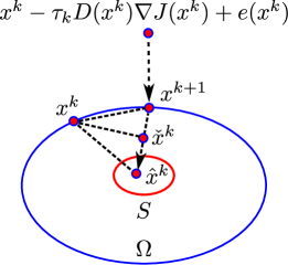
Figure 1: An illustration of the geometric relationship between points $x^{k}$, $x^{k+1}$, $\check{x}^{k}$ and $\hat{x}^{k}$

Since $\Omega$ is convex and $x^{k+1}$ is the projection of $x^{k}-\tau_{k}D(x^{k})\nabla J(x^{k})+e^{k}$ onto $\Omega$ (See Fig. 1), by Lemma 3.2 (i), the following inequality holds

$$\langle x^{k}-\tau_{k}D(x^{k})\nabla J(x^{k})+e(x^{k})-x^{k+1},x^{k+1}-\hat{x}^{k}\rangle\geq 0,$$ (78)

and arrangement of the terms leads to

$$\quad~{}\langle\nabla J(x^{k}),x^{k+1}-\hat{x}^{k}\rangle$$

$$\leq\langle\theta^{k}+\frac{1}{\tau_{k}}e^{k},x^{k+1}-\hat{x}^{k}\rangle+\frac{1}{\tau_{k}}\langle x^{k}-x^{k+1},x^{k+1}-\hat{x}^{k}\rangle$$

$$\leq\left(\|\theta^{k}\|+\frac{1}{\underline{\tau}}\|e^{k}\|+\frac{1}{\underline{\tau}}\|x^{k}-x^{k+1}\|\right)\|x^{k+1}-\hat{x}^{k}\|,$$ (79)

where $\displaystyle\underline{\tau}:=\inf_{k}\tau_{k}$, as defined in (58). By using the mean value theorem again, there is an $\check{x}^{k}$ lying in the line segment between $x^{k+1}$ and $\hat{x}^{k}$ such that

$$J(x^{k+1})-J(\hat{x}^{k})=\langle\nabla J(\check{x}^{k}),x^{k+1}-\hat{x}^{k}\rangle.$$ (80)

Combining (3.2) and (80), yields, in view of (74) and (77), since we are looking at $k>K_{3}>K_{2}>K_{1}$,

$$\quad~{}J(x^{k+1})-J^{\ast}$$

$$=J(x^{k+1})-J(\hat{x}^{k})$$

$$=\langle\nabla J(\check{x}^{k})-\nabla J(x^{k}),x^{k+1}-\hat{x}^{k}\rangle+\langle\nabla J(x^{k}),x^{k+1}-\hat{x}^{k}\rangle$$

$$\leq\|\nabla J(\check{x}^{k})-\nabla J(x^{k})\|\|x^{k+1}-\hat{x}^{k}\|+\langle\nabla J(x^{k}),x^{k+1}-\hat{x}^{k}\rangle$$

$$\leq\left(L\|\check{x}^{k}-x^{k}\|+\|\theta^{k}\|+\frac{1}{\underline{\tau}}\|e^{k}\|+\frac{1}{\underline{\tau}}\|x^{k}-x^{k+1}\|\right)\|x^{k+1}-\hat{x}^{k}\|.\text{ }$$ (81)

To finish the proof we further bound from above the right-hand side of (81). For the term $\|\check{x}^{k}-x^{k}\|$, we note that $\check{x}^{k}$ is in the line segment between $x^{k+1}$ and $\hat{x}^{k},$ thus,

$$\|x^{k+1}-\check{x}^{k}\|+\|\check{x}^{k}-\hat{x}^{k}\|=\|x^{k+1}-\hat{x}^{k}\|\leq\|x^{k}-x^{k+1}\|+\|x^{k}-\hat{x}^{k}\|,$$ (82)

which, when combined with

$$\|\check{x}^{k}-x^{k}\|\leq\|x^{k}-x^{k+1}\|+\|x^{k+1}-\check{x}^{k}\|,$$ (83)

and

$$\|\check{x}^{k}-x^{k}\|\leq\|x^{k}-\hat{x}^{k}\|+\|\hat{x}^{k}-\check{x}^{k}\|,$$ (84)

yields

$$\|\check{x}^{k}-x^{k}\|\leq\|x^{k}-x^{k+1}\|+\|x^{k}-\hat{x}^{k}\|.$$ (85)

On the other hand, (71) and (62) allows us to write

$$\|x^{k}-\hat{x}^{k}\|\leq\beta\eta_{2}(\|x^{k}-x^{k+1}\|+\|e^{k}\|+\|\theta^{k}\|),\quad\text{for all }k>K_{3}.$$ (86)

Thus, we have for the term $L\|\check{x}^{k}-x^{k}\|$, using (85) and (86),

$$L\|\check{x}^{k}-x^{k}\| \leq L\left(\|x^{k}-x^{k+1}\|+\|x^{k}-\hat{x}^{k}\|\right)$$

$$\leq L\left(\|x^{k}-x^{k+1}\|+\beta\eta_{2}(\|x^{k}-x^{k+1}\|+\|e^{k}\|+\|\theta^{k}\|)\right)$$

$$\leq L(1+\beta\eta_{2})(\|x^{k}-x^{k+1}\|+\|e^{k}\|+\|\theta^{k}\|).$$ (87)

For the term $\|x^{k+1}-\hat{x}^{k}\|$ in (3.2), we use the triangle inequality and (86) to get

$$\|x^{k+1}-\hat{x}^{k}\| \leq\|x^{k}-x^{k+1}\|+\|x^{k}-\hat{x}^{k}\|$$

$$\leq\|x^{k}-x^{k+1}\|+\beta\eta_{2}(\|x^{k}-x^{k+1}\|+\|e^{k}\|+\|\theta^{k}\|)$$

$$\leq(1+\beta\eta_{2})(\|x^{k}-x^{k+1}\|+\|e^{k}\|+\|\theta^{k}\|).$$ (88)

Finally, the term $\displaystyle\|\theta^{k}\|+\displaystyle\frac{1}{\underline{\tau}}\|e^{k}\|+\displaystyle\frac{1}{\underline{\tau}}\|x^{k}-x^{k+1}\|$ in the right-hand side of (81) can also be bounded above by

$$\|\theta^{k}\|+\displaystyle\frac{1}{\underline{\tau}}\|e^{k}\|+\displaystyle\frac{1}{\underline{\tau}}\|x^{k}-x^{k+1}\|\leq(1+\displaystyle\frac{1}{\underline{\tau}})(\|x^{k}-x^{k+1}\|+\|e^{k}\|+\|\theta^{k}\|).$$ (89)

Defining

$$\eta_{3}:=(L+L\beta\eta_{2}+1+\frac{1}{\underline{\tau}})(1+\beta\eta_{2}),$$ (90)

and using all the bounds from above, i.e., (81), (85), (86) and (3.2), we obtain

$$J(x^{k+1})-J^{\ast}\leq\eta_{3}\left(\|x^{k}-x^{k+1}\|+\|e^{k}\|+\|\theta^{k}\|\right)^{2},\text{ for all }k>K_{3},$$ (91)

which completes the proof.

Combining Theorem 3.1, Proposition 3.2 and Proposition 3.4, it can be seen that $\lim_{k\rightarrow\infty}J(x^{k})=J^{\ast}$. As an immediate application of the Proposition 3.4, we get the following intermediate proposition that leads to the final result.

Proposition 3.5

Under the conditions of Proposition 3.1, if $\{x^{k}\}_{k=0}^{\infty}$ is any sequence generated by the PSG method with bounded outer perturbations of (29), and if $\displaystyle\lambda_{k}:=\sqrt{J(x^{k})-J^{\ast}}$ for all $k\geq 0$, then $\displaystyle\sum_{k=0}^{\infty}\lambda_{k}<+\infty$.

Proof

There exist real numbers $0<\eta_{4}<1$ and $\eta_{5}>0$ such that

$$\sqrt{J(x^{k+1})-J^{\ast}}\leq\eta_{4}\sqrt{J(x^{k})-J^{\ast}}+\eta_{5}(\|e^{k}\|+\|\theta^{k}\|).$$ (92)

To prove this claim, we use $(a+b)^{2}\leq 2(a^{2}+b^{2})$ and (68) to get

$$J(x^{k+1})-J^{\ast} \leq\eta_{3}\left(\|x^{k}-x^{k+1}\|+\|e^{k}\|+\|\theta^{k}\|\right)^{2}$$

$$\leq 2\eta_{3}\|x^{k}-x^{k+1}\|^{2}+2\eta_{3}(\|e^{k}\|+\|\theta^{k}\|)^{2},$$ (93)

then apply (61),with added and subtracted $J^{\ast},$ to obtain

$$J(x^{k+1})-J^{\ast} \leq\frac{4\eta_{3}}{\eta_{1}}\left(J(x^{k})-J^{\ast}\right)-\frac{4\eta_{3}}{\eta_{1}}\left(J(x^{k+1})-J^{\ast}\right)+\frac{2\eta_{3}}{\eta_{1}^{2}}\|\delta^{k}\|^{2}$$

$$~{}~{}~{}+2\eta_{3}(\|e^{k}\|+\|\theta^{k}\|)^{2}.$$ (94)

Rearranging terms yields

$$J(x^{k+1})-J^{\ast} \leq \frac{4\eta_{3}}{\eta_{1}+4\eta_{3}}\left(J(x^{k})-J^{\ast}\right)+\frac{2\eta_{3}}{\eta_{1}(\eta_{1}+4\eta_{3})}\|\delta^{k}\|^{2}$$ (95)

$$+\frac{2\eta_{1}\eta_{3}}{\eta_{1}+4\eta_{3}}(\|e^{k}\|+\|\theta^{k}\|)^{2}.$$

On the other hand, (58) leads to

$$\|\delta^{k}\|^{2}\leq\frac{1}{\underline{\tau}^{2}}\|e^{k}\|^{2}+\|\theta^{k}\|^{2}\leq\frac{1}{\hat{\tau}^{2}}\left(\|e^{k}\|^{2}+\|\theta^{k}\|^{2}\right)$$ (96)

with $\displaystyle\underline{\tau}:=\inf_{k}\tau_{k}$ and $\displaystyle\hat{\tau}:=\min\{1,\inf_{k}\tau_{k}\}>0$ as defined earlier. Therefore,

$$J(x^{k+1})-J^{\ast} \leq \frac{4\eta_{3}}{\eta_{1}+4\eta_{3}}\left(J(x^{k})-J^{\ast}\right)$$ (97)

$$+\left(\frac{2\eta_{3}}{\eta_{1}(\eta_{1}+4\eta_{3})}\frac{1}{\hat{\tau}^{2}}+\frac{2\eta_{1}\eta_{3}}{\eta_{1}+4\eta_{3}}\right)(\|e^{k}\|+\|\theta^{k}\|)^{2}.$$

Using $\displaystyle\sqrt{a+b}\leq\sqrt{a}+\sqrt{b}$ gives

$$\sqrt{J(x^{k+1})-J^{\ast}} \leq \sqrt{\frac{4\eta_{3}}{\eta_{1}+4\eta_{3}}}\sqrt{J(x^{k})-J^{\ast}}$$ (98)

$$+\sqrt{\frac{2\eta_{3}}{\eta_{1}(\eta_{1}+4\eta_{3})}\frac{1}{\hat{\tau}^{2}}+\frac{2\eta_{1}\eta_{3}}{\eta_{1}+4\eta_{3}}}\left(\|e^{k}\|+\|\theta^{k}\|\right).$$

Denoting $\displaystyle\eta_{4}:=\sqrt{\frac{\displaystyle 4\eta_{3}}{\displaystyle\eta_{1}+4\eta_{3}}}$ and $\displaystyle\eta_{5}:=\sqrt{\frac{\displaystyle 2\eta_{3}}{\displaystyle\eta_{1}(\eta_{1}+4\eta_{3})}\frac{\displaystyle 1}{\displaystyle\hat{\tau}^{2}}+\frac{\displaystyle 2\eta_{1}\eta_{3}}{\displaystyle\eta_{1}+4\eta_{3}}}$, we obtain (92) and, from the definition of $\eta_{4}$ and the fact that $\eta_{1}>0,\eta_{3}>0$,

$$0<\eta_{4}<1.$$ (99)

It follows from (92) that

$$\lambda_{k+1}\leq\eta_{4}\lambda_{k}+\eta_{5}(\|e^{k}\|+\|\theta^{k}\|).$$ (100)

Then, for all $M>N$,

$$\sum_{k=N+1}^{M}\lambda_{k} =\sum_{k=N}^{M-1}\lambda_{k+1}$$

$$\leq\eta_{4}\sum_{k=N}^{M-1}\lambda_{k}+\eta_{5}\sum_{k=N}^{M-1}(\|e^{k}\|+\|\theta^{k}\|)$$

$$\leq\eta_{4}\lambda_{N}+\eta_{4}\sum_{k=N+1}^{M}\lambda_{k}+\eta_{5}\sum_{k=N}^{M}(\|e^{k}\|+\|\theta^{k}\|).$$ (101)

Consequently,

$$\sum_{k=N+1}^{M}\lambda_{k}\leq\frac{\eta_{4}}{1-\eta_{4}}\lambda_{N}+\frac{\eta_{5}}{1-\eta_{4}}\sum_{k=N}^{M}(\|e^{k}\|+\|\theta^{k}\|).$$ (102)

And hence,

$$\sum_{k=N+1}^{\infty}\lambda_{k}\leq\frac{\eta_{4}}{1-\eta_{4}}\lambda_{N}+\frac{\eta_{5}}{1-\eta_{4}}\sum_{k=N}^{\infty}(\|e^{k}\|+\|\theta^{k}\|).$$ (103)

The proof now follows by (31), (33).

Finally, we are ready to prove that sequences generated by the PSG method with bounded outer perturbations of (29) converge to a stationary point in $S$. We do this by combining Proposition 3.2, Proposition 3.3 and Proposition 3.5.

Theorem 3.2

Under the conditions of Proposition 3.1, if $\{x^{k}\}_{k=0}^{\infty}$ is any sequence generated by the PSG method with bounded outer perturbations of (29), then it converges to a stationary point of the problem (1), i.e., to a point in $S$.

Proof

Obviously,

$$|J(x^{k})-J(x^{k+1})|^{1/2} \leq\left(|J(x^{k})-J^{\ast}|+|J(x^{k+1})-J^{\ast}|\right)^{1/2}$$

$$\leq\lambda_{k}+\lambda_{k+1},$$ (104)

which implies, by Proposition 3.5, that

$$\sum_{k=0}^{\infty}|J(x^{k})-J(x^{k+1})|^{1/2}<+\infty.$$ (105)

This, along with Proposition 3.2, guarantees that

$$\sum_{k=0}^{\infty}\|x^{k}-x^{k+1}\|<+\infty,$$ (106)

which implies that the sequence $\{x^{k}\}_{k=0}^{\infty}$ generated by (29)–(33) converges. Denoting $x^{\ast}:=\lim_{k\rightarrow\infty}x^{k}$ and using Proposition 3.3 we get from (62) that $\|r(x^{\ast})\|=0$, i.e., $x^{\ast}\in S$, and the proof is complete.

4 Bounded Perturbation Resilience of PSG Methods

In this section, we prove the bounded perturbation resilience (BPR) of PSG methods. This property is fundamental for the application of the superiorization methodology (SM) to them. We do this by establishing a relationship between BPR and bounded outer perturbations given by (3)–(4).

4.1 Bounded Perturbation Resilience

The superiorization methodology (SM) of Censor2010Perturbation ; Censor2013Projected ; Herman2012Superiorization is intended for nonlinear constrained minimization (CM) problems of the form:

$$\mathrm{minimize}\left\{\phi(x)\mid x\in\Psi\right\},$$ (107)

where $\phi:\mathbb{R}^{n}\rightarrow\mathbb{R}$ is an objective function and $\Psi\subseteq{\mathbb{R}^{n}}$ is the solution set of another problem. The set $\Psi$ could be the solution set of a convex feasibility problem (CFP) of the form: find a vector $x^{\ast}\in\Psi:=\cap_{i=1}^{I}C_{i},$ where the sets $C_{i}\subseteq\mathbb{R}^{n}$ ($1\leq i\leq I$) are closed convex subsets of the Euclidean space $\mathbb{R}^{n}$, see, e.g., Bauschke1996projection ; Byrne2008Applied ; Chinneck2008Feasibility or (Censor1997Parallel, , Chapter 5) for results and references on this broad topic. In such a case we deal in (107) with a standard CM problem. Here we are interested in the case wherein $\Psi$ is the solution set of another CM, namely the one presented at the beginning of the paper,

$$\mathrm{minimize}\left\{J(x)\mid x\in\Omega\right\},$$ (108)

i.e., we wish to look at,

$$\Psi:=\left\{x^{\ast}\in\Omega\mid J(x^{\ast})\leq J(x)\text{ for all }x\in\Omega\right\},$$ (109)

assuming that $\Psi$ is nonempty.

In either case, or any other case of the set $\Psi$, the SM strives not to solve (107) but rather the task is to find a point in $\Psi$ that is superior (i.e., has a lower, but not necessarily minimal, value of the $\phi$ objective function value) to one returned by an algorithm that solves (108) alone. This is done in the SM by first investigating the bounded perturbation resilience of an algorithm designed to solve (108) and then proactively using such permitted perturbations in order to steer the iterates of such an algorithm toward lower values of the $\phi$ objective function while not loosing the overall convergence to a point in $\Psi$. See Censor2010Perturbation ; Censor2013Projected ; Herman2012Superiorization for details of the SM. A recent review of superiorization-related previous work appears in (Censor2013Projected, , Section 3).

In this paper we do not perform superiorization of any algorithm. Such superiorization of the EM algorithm with total variation (TV) serving as the $\phi$ objective function and an application of the approach to an inverse problem of image reconstruction for bioluminescence tomography will be presented in a sequel paper. Our aim here is to pave the way for such an application by proving the bounded perturbation resilience that is needed in order to do superiorization.

For technical reasons that will become clear as we proceed, we introduce an additional set $\Theta$ such that $\Psi\subseteq\Theta\subseteq{\mathbb{R}^{n}}$ and assume that we have an algorithmic operator $\boldsymbol{A}_{\Psi}:\mathbb{R}^{n}\rightarrow\Theta$, that defines a Basic Algorithm as follows.

Algorithm 4.1

The Basic Algorithm

Initialization: $x^{0}\in\Theta$ is arbitrary;

Iterative Step: Given the current iterate vector $x^{k}$, calculate the next iterate $x^{k+1}$ by

$$x^{k+1}=\boldsymbol{A}_{\Psi}\left(x^{k}\right).$$ (110)

The bounded perturbation resilience (henceforth abbreviated by BPR) of such a basic algorithm is defined next.

Definition 4.2

Bounded Perturbation Resilience (BPR) An algorithmic operator $\boldsymbol{A}_{\Psi}:\mathbb{R}^{n}\rightarrow\Theta$ is said to be bounded perturbations resilient if the following holds. If Algorithm 4.1 generates sequences $\{x^{k}\}_{k=0}^{\infty}$ with $x^{0}\in\Theta,$ that converge to points in $\Psi,$ then any sequence $\{y^{k}\}_{k=0}^{\infty}$, starting from any $y^{0}\in\Theta$, generated by

$$y^{k+1}=\boldsymbol{A}_{\Psi}\left(y^{k}+\beta_{k}v^{k}\right),\text{ for all }k\geq 0,$$ (111)

where ($i$) the vector sequence $\{v^{k}\}_{k=0}^{\infty}$ is bounded, and ($ii$) the scalars $\{\beta_{k}\}_{k=0}^{\infty}$ are such that $\beta_{k}\geq 0$ for all $k\geq 0$, and ${\sum_{k=0}^{\infty}}\beta_{k}<\infty,$ and ($iii$) $y^{k}+\beta_{k}v^{k}\in\Theta$ for all $k\geq 0,$ also converges to a point in $\Psi$.

Comparing this definition with (Censor2010Perturbation, , Definition 1), (Herman2012Superiorization, , Subsection II.C) and (Censor2013Projected, , Definition 4.2), we observe that ($iii$) in Definition 4.2 above is needed only if $\Theta\neq\mathbb{R}^{n}$. In that case, the condition ($iii$) of Definition 4.2 above is enforced in the superiorized version of the basic algorithm, see step (xiv) in the “Superiorized Version of Algorithm P” in (Herman2012Superiorization, , p. 5537) and step (14) in “Superiorized Version of the ML-EM Algorithm” in (Garduno2013Superiorization, , Subsection II.B). This will be the case in the present work.

An important special case, from which the superiorization methodology originally grew and developed, is when $\Psi$ is the solution set of the (linear) convex feasibility problem and $A_{\Psi}$ is a string-averaging projection method. This was discussed and experimented with for problems of image reconstruction from projections wherein the function $\phi$ of (107) was the total variation (TV) of the image vector $x,$ see Butnariu2007Stable ; Davidi2009Perturbation .

Note also that in later works Censor2013Projected ; Herman2012Superiorization the notion of BPR was replaced by that of strong perturbation resilience which caters to situations where $\Psi$ might be empty, however we still work here with the above asymptotic notion of BPR and assume that $\Psi$ is nonempty. Treating the PSG method as the Basic Algorithm $A_{\Psi}$, our strategy was to first prove convergence of the PSG iterative algorithm with bounded outer perturbations, i.e., convergence of

$$x^{k+1}=P_{\Omega}(x^{k}-\tau_{k}D(x^{k})\nabla J(x^{k})+e^{k}).$$ (112)

We show next how the convergence of this yields BPR according to Definition 4.2. Such a two steps strategy was also applied in (Butnariu2007Stable, , p. 541).

A superiorized version of any Basic Algorithm employs the perturbed version of the Basic Algorithm as in (111). A certificate to do so in the superiorization method, see censor-weak-14 , is gained by showing that the Basic Algorithm is BPR (or strongly perturbation resilient, a notion not discussed in the present paper). Therefore, proving the BPR of an algorithm is the first step toward superiorizing it. This is done for the PSG method in the next subsection.

4.2 The BPR of PSG Methods as a Consequence of Bounded Outer Perturbation Resilience

In this subsection, we prove the BPR of the PSG method whose iterative step is given by (6). To this end we treat the right-hand side of (6) as the algorithmic operator $\boldsymbol{A}_{\Psi}$ of Definition 4.2, namely, we define for all $k\geq 0$,

$$\boldsymbol{A}_{\Psi}\left(x^{k}\right):=P_{\Omega}(x^{k}-\tau_{k}D(x^{k})\nabla J(x^{k})),$$ (113)

and identify the solution set $\Psi$ there with the set $S$ of (26), and identify the additional set $\Theta$ there with the constraint set $\Omega$ of (1).

According to Definition 4.2, we need to show convergence of any sequence $\{x^{k}\}_{k=0}^{\infty}$ that, starting from any $x^{0}\in\Omega$, is generated by

$$x^{k+1} =P_{\Omega}\left((x^{k}+\beta_{k}v^{k})-\tau_{k}D(x^{k}+\beta_{k}v^{k})\nabla J(x^{k}+\beta_{k}v^{k})\right),$$ (114)

for all $k\geq 0$, to a point in $S$ of (26), where $\{v^{k}\}_{k=0}^{\infty}$ and $\{\beta_{k}\}_{k=0}^{\infty}$ obey the conditions ($i$) and ($ii$) in Definition 4.2, respectively, and also ($iii$) in Definition 4.2 holds.

The next theorem establishes the bounded perturbation resilience of the PSG methods. The proof idea is to build a relationship between BPR and the convergence of PSG methods with bounded outer perturbations of (3)–(4).

We caution the reader that we introduce below the assumption that the set $\Omega$ is bounded. This forces us to modify the problems (8) and (18) by replacing $\Omega_{0}$ with some bounded subset of it in order to apply our results. While this is admittedly a mathematically weaker result than we hoped for, we note that this would not be a harsh limitation in practical applications wherein such boundedness can be achieved from problem-related practical considerations.

Theorem 4.1

Given a nonempty closed convex and bounded set $\Omega\subseteq\mathbb{R}^{n}$, assume that $J\in\mathcal{S}_{\mu,L}^{1,1}(\Omega)$ (i.e., $J$ obeys (27) and (28)) and there exists at least one point $x_{\Omega}\in\Omega$ such that $\|\nabla J(x_{\Omega})\|<+\infty$. Let $\{\tau_{k}\}_{k=0}^{\infty}$ be a sequence of positive scalars that fulfills (30), $\{D(x)\}_{k=0}^{\infty}$ be a sequence of diagonal scaling matrices that is either of form (16) or (24), and let $\{\theta^{k}\}_{k=0}^{\infty}$ be as in (32) and for which (33) holds. Under these assumptions, if the vector sequence $\{v^{k}\}_{k=0}^{\infty}$ is bounded and the scalars $\{\beta_{k}\}_{k=0}^{\infty}$ are such that $\beta_{k}\geq 0$ for all $k\geq 0$, and $\sum_{k=0}^{\infty}\beta_{k}<\infty$, then, for any $x^{0}\in\Omega$, any sequence $\{x^{k}\}_{k=0}^{\infty}$, generated by (114) such that $x^{k}+\beta_{k}v^{k}\in\Omega$ for all $k\geq 0$, converges to a point in $S$ of (26).

Proof

The proof is in two steps. For the first step, we build a relationship between (114) and bounded outer perturbations of (3)–(4). For the second step, we invoke Theorem 3.2 and establish the convergence result.
Step 1. We show that any sequence generated by (114) satisfies

$$x^{k+1}=P_{\Omega}\left(x^{k}-\tau_{k}D(x^{k})\nabla J(x^{k})+e^{k}\right),$$ (115)

with $\sum_{k=0}^{\infty}\|e^{k}\|<+\infty$. Since $\Omega$ is a bounded subset of $\mathbb{R}^{n}$, there exists a $r_{\Omega}>0$ such that $\Omega\subseteq B(x_{\Omega},r_{\Omega})$, where $B(x_{\Omega},r_{\Omega})\subseteq\mathbb{R}^{n}$ is a ball centered at $x_{\Omega}$ with radius $r_{\Omega}$. Then, for any $x\in\Omega$,

$$\|x-x_{\Omega}\|\leq r_{\Omega}~{}\Rightarrow~{}\|x\|\leq\|x_{\Omega}\|+r_{\Omega}.$$ (116)

The Lipschitzness of $\nabla J(x)$ on $\Omega$ and (116) imply that, for any $x\in\Omega$,

$$\|\nabla J(x)-\nabla J(x_{\Omega})\|\leq L\|x-x_{\Omega}\|\Rightarrow\|\nabla J(x)\|\leq\|\nabla J(x_{\Omega})\|+Lr_{\Omega}.$$ (117)

Since the sequence $\{x^{k}\}_{k=0}^{\infty}$ generated by (114) is contained in $\Omega$, due to the projection operation $P_{\Omega}$, and $x^{k}+\beta_{k}v^{k}$ is also in $\Omega$, it holds that, for all $k\geq 0$, $x^{k}$ and $x^{k}+\beta_{k}v^{k}$ satisfy (116), and that $\nabla J(x^{k})$ and $\nabla J(x^{k}+\beta_{k}v^{k})$ satisfy (117). Besides, the boundness of ${\{v^{k}\}}_{k=0}^{\infty}$ implies that there exist a $\overline{v}>0$ such that $\|v^{k}\|\leq\overline{v}$ for all $k\geq 0$. Therefore, we have

$$\|\beta_{k}v^{k}\|\leq\overline{v}\beta_{k}.$$ (118)

From (114), the outer perturbation term $e^{k}$ of (115) is given by

$$e^{k} =\left(x^{k}+\beta_{k}v^{k}-\tau_{k}D(x^{k}+\beta_{k}v^{k})\nabla J(x^{k}+\beta_{k}v^{k})\right)-\left(x^{k}-\tau_{k}D(x^{k})\nabla J(x^{k})\right)$$

$$=\beta_{k}v^{k}+\tau_{k}\left(D(x^{k})\nabla J(x^{k})-D(x^{k}+\beta_{k}v^{k})\nabla J(x^{k}+\beta_{k}v^{k})\right).$$ (119)

Given that $D(x)$ is either of form (16) or (24), we consider them separately. In what follows, we repeatedly use the fact that $\|ABx\|\leq\|AB\|_{F}\|x\|\leq\|A\|_{F}\|B\|_{F}\|x\|$ for any $A,B\in\mathbb{R}^{n\times n}$ and $x\in\mathbb{R}^{n}$, with $\|\cdot\|_{F}$ the Frobenius norm of matrix, see, e.g., (Golub1996Matrix, , Section 2.3).

($i$)

Assume that $D(x)$ is of form (16), namely that $D(x)\equiv D_{\mathrm{LS}}$ for any $x$. For this case, combining (4.2) with (27), (30) and (118), and by the Minkowski inequality, we get

$$\|e^{k}\| =\|\beta_{k}v^{k}+\tau_{k}D_{\mathrm{LS}}\left(\nabla J(x^{k})-\nabla J(x^{k}+\beta_{k}v^{k})\right)\|$$

$$\leq\|\beta_{k}v^{k}\|+\tau_{k}\|D_{\mathrm{LS}}\|_{F}\|\nabla J(x^{k})-\nabla J(x^{k}+\beta_{k}v^{k})\|$$

$$\leq\|\beta_{k}v^{k}\|+\tau_{k}\|D_{\mathrm{LS}}\|_{F}L\|\beta_{k}v^{k}\|$$

$$\leq(1+2\|D_{\mathrm{LS}}\|_{F})\overline{v}\beta_{k}.$$ (120)

($ii$)

Assume that $D(x)$ is of form (24), namely that $D(x):=\hat{D}X$ with $\hat{D}=\operatorname*{diag}\{1/\hat{s}_{j}\}$ and $X=\operatorname*{diag}\{x_{j}\}$ diagonal matrices. In this case, combining (4.2) with (27), (30), (116), (117), (118), and by the Minkowski inequality, we get

$$\|e^{k}\| =\|\beta_{k}v^{k}+\tau_{k}\left(D(x^{k})\nabla J(x^{k})-D(x^{k}+\beta_{k}v^{k})\nabla J(x^{k}+\beta_{k}v^{k})\right)\|$$

$$=\|\beta_{k}v^{k}+\tau_{k}\left(D(x^{k})\nabla J(x^{k})-D(x^{k}+\beta_{k}v^{k})\nabla J(x^{k})\right)$$

$$\quad+\tau_{k}\left(D(x^{k}+\beta_{k}v^{k})\nabla J(x^{k})-D(x^{k}+\beta_{k}v^{k})\nabla J(x^{k}+\beta_{k}v^{k})\right)\|$$

$$\leq\|\beta_{k}v^{k}\|+\tau_{k}\|\hat{D}(X^{k}-\hat{X}^{k})\nabla J(x^{k})\|$$

$$\quad+\tau_{k}\|\hat{D}\hat{X}^{k}(\nabla J(x^{k})-\nabla J(x^{k}+\beta_{k}v^{k}))\|$$

$$\leq\|\beta_{k}v^{k}\|+\tau_{k}\|\hat{D}\|_{F}\|X^{k}-\hat{X}^{k}\|_{F}\|\nabla J(x^{k})\|+\tau_{k}\|\hat{D}\hat{X}^{k}\|_{F}L\|\beta_{k}v^{k}\|$$

$$\leq(1+\tau_{k}\|\hat{D}\|_{F}\|\nabla J(x^{k})\|+\tau_{k}L\|\hat{D}\|_{F}\|\hat{X}^{k}\|_{F})\|\beta_{k}v^{k}\|$$ (121)

$$\leq(1+2\|\hat{D}\|_{F}\|\nabla J(x^{k})\|/L+2\|\hat{D}\|_{F}\|x^{k}+\beta_{k}v^{k}\|)\overline{v}\beta_{k}$$ (122)

$$\leq\left(1+2\|\hat{D}\|_{F}(\|\nabla J(x_{\Omega})\|/L+\|x_{\Omega}\|+2r_{\Omega})\right)\overline{v}\beta_{k},$$ (123)

where $X^{k}:=\operatorname*{diag}\{x^{k}_{j}\}$, $\hat{X}^{k}:=\operatorname*{diag}\{(x^{k}+\beta_{k}v^{k})_{j}\}$, and (121) holds by the fact that $\|X^{k}-\hat{X}^{k}\|_{F}=\|x^{k}-(x^{k}+\beta_{k}v^{k})\|=\|\beta_{k}v^{k}\|$, and (122) holds since $\|\hat{X}^{k}\|_{F}=\|x^{k}+\beta_{k}v^{k}\|$, and (123) holds by (116) and (117).

Defining a constant

$$C_{\Omega}:=\overline{v}+2\overline{v}\cdot\max\left\{\|D_{\mathrm{LS}}\|_{F},~{}\|\hat{D}\|_{F}(\|\nabla J(x_{\Omega})\|/L+\|x_{\Omega}\|+2r_{\Omega})\right\},$$ (124)

and considering (($i$)) or (123), yields that in either case ($i$) or case ($ii$),

$$\|e^{k}\|\leq C_{\Omega}\beta_{k}.$$ (125)

Then, $\sum_{k=0}^{\infty}\beta_{k}<+\infty$ implies that $\sum_{k=0}^{\infty}\|e^{k}\|<+\infty$.
Step 2. Under the given conditions, by invoking Theorem 3.2, we know that, for any $x^{0}\in\Omega$, any sequence $\{x^{k}\}_{k=0}^{\infty}$, generated by (115) in which $\sum_{k=0}^{\infty}\|e^{k}\|<+\infty$, converges to a point in $S$ of (26). Hence, the sequence generated by (114) also converges to the same point of $S$.

References

- (1) Bauschke, H.H., Borwein, J.M.: On projection algorithms for solving convex feasibility problems. SIAM Rev. 38, 367–426 (1996)
- (2) Bertero, M., Boccacci, P.: Introduction to Inverse Problems in Imaging. Institute of Physics, Bristol, UK (1998)
- (3) Bertero, M., Lantéri, H., Zanni, L.: Iterative image reconstruction: a point of view. In: Censor, Y., Jiang, M., Louis, A.K. (eds.) Mathematical Methods in Biomedical Imaging and Intensity-Modulated Radiation Therapy (IMRT), Publications of the Scuola Normale Superiore, vol. 7, pp. 37–63. Edizioni della Normale, Pisa, Italy (2008)
- (4) Bertsekas, D.P.: On the Goldstein-Levitin-Polyak gradient projection method. IEEE Trans. Autom. Control 21, 174–184 (1976)
- (5) Bertsekas, D.P.: Projected Newton methods for optimization problems with simple constraints. SIAM J. Control Optim. 20, 221–246 (1982)
- (6) Bertsekas, D.P.: Nonlinear Programming. Athena Scientific, Belmont, MA, USA (1999)
- (7) Bonettini, S., Zanella, R., Zanni, L.: A scaled gradient projection method for constrained image deblurring. Inverse Probl. 25, 015002 (23pp) (2009)
- (8) Butnariu, D., Davidi, R., Herman, G.T., Kazantsev, I.G.: Stable convergence behavior under summable perturbations of a class of projection methods for convex feasibility and optimization problems. IEEE J. Sel. Top. Signal Process. 1, 540–547 (2007)
- (9) Byrne, C.L., Censor, Y.: Proximity function minimization using multiple Bregman projections, with applications to split feasibility and Kullback-Leibler distance minimization. Ann. Oper. Res. 105, 77–98 (2001)
- (10) Byrne, C.L.: Iterative image reconstruction algorithms based on cross-entropy minimization. IEEE Trans. Image Process. 2, 96–103 (1993)
- (11) Byrne, C.L.: Applied Iterative Methods. A K Peters, Wellesley, MA, USA (2008)
- (12) Cegielski, A.: Iterative Methods for Fixed Point Problems in Hilbert Spaces, Lecture Notes in Mathematics, vol. 2057. Springer, Heidelberg, Germany (2013)
- (13) Censor, Y.: Weak and strong superiorization: Between feasibility-seeking and minimization. An. St. Univ. Ovidius Constanta, Ser. Mat., accepted for publication. http://arxiv.org/abs/1410.0130.
- (14) Censor, Y., Davidi, R., Herman, G.T.: Perturbation resilience and superiorization of iterative algorithms. Inverse Probl. 26, 065008 (12pp) (2010)
- (15) Censor, Y., Davidi, R., Herman, G.T., Schulte, R.W., Tetruashvili, L.: Projected subgradient minimization versus superiorization. J. Optim. Theory Appl. 160, 730–747 (2014)
- (16) Censor, Y., Elfving, T., Herman, G.T., Nikazad, T.: On diagonally relaxed orthogonal projection methods. SIAM J. Sci. Comput. 30, 473–504 (2008)
- (17) Censor, Y., Zaslavski, A.J.: Convergence and perturbation resilience of dynamic string-averaging projection methods. Comput. Optim. Appl. 54, 65–76 (2013)
- (18) Censor, Y., Zenios, S.A.: Parallel Optimization: Theory, Algorithms, and Applications. Oxford University Press, New York, NY, USA (1997)
- (19) Cheng, Y.C.: On the gradient-projection method for solving the nonsymmetric linear complementarity problem. J. Optim. Theory Appl. 43, 527–541 (1984)
- (20) Chinneck, J.W.: Feasibility and Infeasibility in Optimization: Algorithms and Computational Methods. International Series in Operations Research and Management Science, vol. 118. Springer, New York, NY, USA (2008)
- (21) Combettes, P.L.: Inconsistent signal feasibility problems: Least-squares solutions in a product space. IEEE Trans. Signal Process. 42, 2955–2966 (1994)
- (22) Combettes, P.L.: Quasi-Fejérian analysis of some optimization algorithms. In: Butnariu, D., Censor, Y., Reich, S. (eds.) Inherently Parallel Algorithms in Feasibility and Optimization and their Applications, Studies in Computational Mathematics, vol. 8, pp. 115–152. Elsevier, Amsterdam, The Netherlands (2001)
- (23) Csiszár, I.: Why least squares and maximum entropy? An axiomatic approach to inference for linear inverse problems. Ann. Statist. 19, 2032–2066 (1991)
- (24) Davidi, R., Herman, G.T., Censor, Y.: Perturbation-resilient block-iterative projection methods with application to image reconstruction from projections. Int. Trans. Oper. Res. 16, 505–524 (2009)
- (25) Gafni, E.M., Bertsekas, D.P.: Two-metric projection methods for constrained optimization. SIAM J. Control Optim. 22, 936–964 (1984)
- (26) Garduño, E., Herman, G.T.: Superiorization of the ML-EM algorithm. IEEE Trans. Nucl. Sci. 61, 162–172 (2014)
- (27) Goldstein, A.A.: Convex programming in Hilbert space. Bull. Amer. Math. Soc. 70, 709–710 (1964)
- (28) Golub, G.H., Van Loan, C.F.: Matrix Computations, 3rd edn. Johns Hopkins University Press, Baltimore, MD, USA (1996)
- (29) Helou Neto, E.S., De Pierro, A.R.: Convergence results for scaled gradient algorithms in positron emission tomography. Inverse Probl. 21, 1905–1914 (2005)
- (30) Helou Neto, E.S., De Pierro, A.R.: Incremental subgradients for constrained convex optimization: a unified framework and new methods. SIAM J. Optim. 20, 1547–1572 (2009)
- (31) Herman, G.T.: Superiorization for image analysis. In: Combinatorial Image Analysis, Lecture Notes in Computer Science, vol. 8466, pp. 1-7. Springer, Switzerland (2014)
- (32) Herman, G.T.: Fundamentals of Computerized Tomography: Image Reconstruction from Projections, 2nd edn. Springer, London, UK (2009)
- (33) Herman, G.T., Garduño, E., Davidi, R., Censor, Y.: Superiorization: An optimization heuristic for medical physics. Med. Phys. 39, 5532–5546 (2012)
- (34) Iusem, A.N.: Convergence analysis for a multiplicatively relaxed EM algorithm. Math. Meth. Appl. Sci. 14, 573–593 (1991)
- (35) Jiang, M., Wang, G.: Development of iterative algorithms for image reconstruction. J. X-Ray Sci. Technol. 10, 77–86 (2001)
- (36) Jiang, M., Wang, G.: Convergence studies on iterative algorithms for image reconstruction. IEEE Trans. Med. Imaging 22, 569–579 (2003)
- (37) Jin, W., Censor, Y., Jiang, M.: A heuristic superiorization-like approach to bioluminescence tomography. In: World Congress on Medical Physics and Biomedical Engineering May 26-31, 2012, Beijing, China, IFMBE Proceedings, vol. 39, pp. 1026–1029. Springer, Heidelberg, Germany (2013)
- (38) Kiwiel, K.C.: Convergence of approximate and incremental subgradient methods for convex optimization. SIAM J. Optim. 14, 807–840 (2004)
- (39) Landweber, L.: An iteration formula for Fredholm integral equations of the first kind. Amer. J. Math. 73, 615–624 (1951)
- (40) Lantéri, H., Roche, M., Cuevas, O., Aime, C.: A general method to devise maximum-likelihood signal restoration multiplicative algorithms with non-negativity constraints. Signal Process. 81, 945–974 (2001)
- (41) Levitin, E.S., Polyak, B.T.: Constrained minimization methods. USSR Comput. Math. Math. Phys. 6, 1–50 (1966)
- (42) Li, W.: Remarks on convergence of the matrix splitting algorithm for the symmetric linear complementarity problem. SIAM J. Optim. 3, 155–163 (1993)
- (43) Luo, S., Zhou, T.: Superiorization of EM algorithm and its application in single-photon emission computed tomography (SPECT). Inverse Probl. Imaging. 8, 223–246 (2014)
- (44) Luo, Z.Q., Tseng, P.: On the linear convergence of descent methods for convex essentially smooth minimization. SIAM J. Control Optim. 30, 408–425 (1992)
- (45) Luo, Z.Q., Tseng, P.: Error bounds and convergence analysis of feasible descent methods: A general approach. Ann. Oper. Res. 46, 157–178 (1993)
- (46) Mangasarian, O.L.: Convergence of iterates of an inexact matrix splitting algorithm for the symmetric monotone linear complementarity problem. SIAM J. Optim. 1, 114–122 (1991)
- (47) McCormick, S.F., Rodrigue, G.H.: A uniform approach to gradient methods for linear operator equations. J. Math. Anal. Appl. 49, 275–285 (1975)
- (48) Nesterov, Y.: Introductory Lectures on Convex Optimization: A Basic Course, Applied Optimization, vol. 87. Springer, New York, NY, USA (2004)
- (49) Nikazad, T., Davidi, R., Herman, G.T.: Accelerated perturbation-resilient block-iterative projection methods with application to image reconstruction. Inverse Probl. 28, 035005 (19pp) (2012)
- (50) Pang, J.S.: A posteriori error bounds for the linearly-constrained variational inequality problem. Math. Oper. Res. 12, 474–484 (1987)
- (51) Pang, J.S.: Error bounds in mathematical programming. Math. Program. 79, 299–332 (1997)
- (52) Penfold, S.N., Schulte, R.W., Censor, Y., Rosenfeld, A.B.: Total variation superiorization schemes in proton computed tomography image reconstruction. Med. Phys. 37, 5887–5895 (2010)
- (53) Piana, M., Bertero, M.: Projected Landweber method and preconditioning. Inverse Probl. 13, 441–463 (1997)
- (54) Polyak, B.T.: Introduction to Optimization. Optimization Software, New York, NY, USA (1987)
- (55) Davidi, R., Censor, Y., Schulte, R.W., Geneser, S., Xing, L.: Feasibility-seeking and superiorization algorithms applied to inverse treatment planning in radiation therapy, Contemp. Math. 636, 83–92 (2015)
- (56) Schrapp, M.J., and Herman, G.T.: Data fusion in X-ray computed tomography using a superiorization approach, Rev. Sci. Instr. 85, 053701 (9pp) (2014)
- (57) Shepp, L.A., Vardi, Y.: Maximum likelihood reconstruction for emission tomography. IEEE Trans. Med. Imaging 1, 113–122 (1982)
- (58) Solodov, M.V.: Convergence analysis of perturbed feasible descent methods. J. Optim. Theory Appl. 93, 337–353 (1997)
- (59) Solodov, M.V., Zavriev, S.K.: Error stability properties of generalized gradient-type algorithms. J. Optim. Theory Appl. 98, 663–680 (1998)
- (60) Trussell, H., Civanlar, M.: The Landweber iteration and projection onto convex sets. IEEE Trans. Acoust. Speech Signal Process. 33, 1632–1634 (1985)