A Social Spider Algorithm for Solving the Non-convex Economic Load Dispatch Problem

Abstract

Economic Load Dispatch (ELD) is one of the essential components in power system control and operation. Although conventional ELD formulation can be solved using mathematical programming techniques, modern power system introduces new models of the power units which are non-convex, non-differentiable, and sometimes non-continuous. In order to solve such non-convex ELD problems, in this paper we propose a new approach based on the Social Spider Algorithm (SSA). The classical SSA is modified and enhanced to adapt to the unique characteristics of ELD problems, e.g., valve-point effects, multi-fuel operations, prohibited operating zones, and line losses. To demonstrate the superiority of our proposed approach, five widely-adopted test systems are employed and the simulation results are compared with the state-of-the-art algorithms. In addition, the parameter sensitivity is illustrated by a series of simulations. The simulation results show that SSA can solve ELD problems effectively and efficiently.

1 Introduction

Economic Load Dispatch (ELD) is a fundamental problem in power system control and operation. The goal for ELD is to find a best feasible power generation schedule with a minimal fuel cost, while satisfying the generation constraints of the power units [1]. In the canonical formulation of ELD, the fuel costs of power units are represented by quadratic functions, which are convex and can be easily solved using mathematical programming methods. Many classical methods have been employed to solve ELD in the past decades, e.g., the gradient method [2], the lambda iteration method [3], and quadratic programming [4]. These methods have also been employed to solve other optimization problems in power system like the Unit Commitment problem [5] and the Optimal Power Flow problem [6].

Although the convex, differentiable, and monotonically increasing canonical formulation of ELD is simple to solve, it is unrealistic because valve-point effects (VPE), multi-fuel options (MFO), and prohibited operating zones (POZ) are not considered. However, all these factors shall be accounted for in the real-world industrial production process. Incorporating these factors, the modern ELD is represented by a non-convex, non-continuous, and non-differentiable optimization problem with many equality and inequality constraints, making it very challenging to find the global optimum solution. For the sake of simplicity, ELD is used to refer to the modern formulation of the problem hereafter.

Despite the complexity of the problem, a number of techniques have been devised to solve ELD in the past decade, e.g., Tabu search [7], Taguchi method [8], and variants of particle swarm optimization [9, 10]. Evolutionary algorithms (EAs) also play an important role in solving ELD problems. Currently most state-of-the-art solvers for ELD are EAs and their variants according to the analysis in [11].

Social Spider Algorithm (SSA) is a recently proposed evolutionary algorithm to solve global numerical optimization problems [12]. By mimicking the foraging behavior of the social spiders, SSA explores and exploits the solution space in an iterative manner. In the formulation of SSA, searching information is propagated among the individuals, i.e., spiders, through the means of vibrations, which are lossy. In addition to this lossy information feature, SSA also incorporates a new social animal foraging model, namely, the information sharing model [13]. In this model, individuals in a population perform searching and joining behaviors simultaneously, which could potentially result in improved searching efficiency [12, 14]. The reasons leading to the outstanding performance of SSA have been investigated in [12], and the improvements are mainly credited to the unique design of the information loss scheme and the searching pattern. Besides its superiority in solving optimization benchmark problems [12], SSA has also demonstrated its potential to be applied to address real world complex optimization problems [15]. This makes it a good candidate to generate outstanding power schedules for ELD.

In this paper, we propose a variant of SSA to solve ELD problem, accounting for VPE, MFO, POZ, and power line loss. The advantage of our proposed algorithm is that it can generate more cost-efficient power schedules when compared with other algorithms. The rest of the paper is organized as follows. We first introduce the related work in Section 2. Section 3 presents the formulation of ELD with VPE, MFO, POZ, and power line loss. Our proposed algorithm is elaborated in Section 4, and simulation problems, results, and comparisons are shown in Section 5. Finally we conclude this paper in Section 6.

2 Related Work

Over the past decades, many methods have been developed to solve ELD. Lin and Viviani proposed a hierarchical numerical method to solve the economic dispatch problem with piecewise quadratic cost functions [16]. In this work the authors considered multiple intersecting cost functions for each generator, which is an analogy of MFO. A similar formulation of the problem is addressed by Park et al. [17] with hopfield neural networks. This work is among the first attempts of adopting computational intelligence methodologies in solving ELD. Lee et al. later proposed an adaptive hopfield neural network to solve the same problem [18]. Their algorithm introduced a slope adjustment and bias adjustment method to speed up the convergence of the hopfield neural network system with adaptive learning rates. Lee and Breipohl proposed a decomposition technique to solve ELD with POZ [19]. Their algorithm decomposes the nonconvex decision space into subsets which can be solved via the conventional Lagrangian relaxation approach. Binetti proposed a distributed algorithm based on the auction techniques and consensus protocols to solve ELD [20]. In their work, each power unit locally evaluates its possible fuel costs as bids. The bids are later employed in the auction mechanism to come up with a consensus. A very recent work by Zhan et al. proposed a dimensional steepest decline method [11]. This method utilizes the local minimum analysis of the ELD problem to reduce the solution space to singular points.

Besides the above non-EA approaches, many EA methods have also been developed to solve various formulations of ELD. Orero and Irving proposed a simple Genetic Algorithm (GA) to solve ELD with POZ [21]. Besides the standard GA, this work also devised a deterministic crowding GA model to solve the problem. Chiang developed an improved GA with the multiplier updating scheme for ELD with VPE and MFO [22]. In this work, the proposed GA is incorporated with an improved evolutionary direction operator. In addition, the tailor-made migration operator efficiently searches the solution space. He et al. proposed a hybrid GA approach to solve ELD with VPE [23]. The algorithm proposed is a hybrid GA with differential evolution (DE) and sequential quadratic programming (SQP). Sinha et al. developed an Evolutionary Programming (EP) method to solve ELP with VPE [24]. Pereira-Neto et al. proposed an Evolutionary Strategy (ES) method to solve ELP with VPE and POZ [25]. DE has also been adapted to solve ELD [26, 27].

Swarm Intelligence (SI), a branch of EA, has also attracted researchers’ attention. Particle Swarm Optimization (PSO) has made a significant contribution in solving ELD problems. Selvakumar and Thanushkodi proposed a “new PSO” based on the classical PSO for ELD with VPE, MFO, and POZ [28]. They manipulated the cognitive searching behavior in PSO to facilitate the solution space exploration. They also proposed an anti-predatory PSO in [29]. In this algorithm, a new anti-predator scheme is modeled and introduced in the classical PSO. Chaturvedi et al. proposed a hierarchical PSO for ELD with VPE and POZ [30]. In this work, a time-varying acceleration coefficient is introduced to act as the inertia factor of PSO. Meng et al. proposed a Quantum PSO for ELD with VPE [31]. Their algorithm demonstrated strong searching ability and fast convergence speed, which are contributed by the introduction of quantum computing theory, self-adaptive probability selection, and chaotic sequence mutation. Safari and Shayeghi developed an Iteration PSO for ELD with VPE and POZ [32]. Besides the conventional global best (gBest) and personal best (pBest) positions considered in canonical PSO, the proposed algorithm also considers an iteration best (iBest) position in the searching process. Nature-inspired EAs also yield satisfactory results in solving ELD variants. Some outstanding ones are Bee Colony Optimization Algorithm [33], Biogeography-Based Optimization [34], Ant Swarm Optimization [35], Harmony Search Algorithm [36], and Chemical Reaction Optimization [37].

3 Economic Load Dispatch Problem

The objective of the ELD problem is to find an optimal power generation schedule with minimal fuel cost while satisfying different power system operating constraints, including power unit and load balancing constraints. In this paper we adopt the formulation described in [11] and [37]. The problem is formulated on one-hour time spans.

3.1 Objective Function

The objective function of ELD is defined as follows:

$$\min_{P}\sum^{n}_{i=1}F_{i}^{c}(P_{i}),$$ (1)

where $n$ is the total number of power units, $F_{i}^{c}(P_{i})$ is the fuel cost function for the $i$th power unit, and $P_{i}$ is the power generation for the $i$th power unit according to the power generation schedule.

3.1.1 Valve-point Effect

Conventionally the fuel cost of power units are formulated by a quadratic function with the following form:

$$F_{i}^{c}=a_{i}+b_{i}P_{i}+c_{i}P_{i}^{2},$$ (2)

where $a$, $b$, and $c$ are constant coefficients determined by the physical characteristics of the power units. However, the fuel cost function exhibits a larger variation in practice due to VPE, which generates ripple like effect during the valve-opening process of multi-valve units. A more precise formulation with both a quadratic component and a rectified sinusoidal component is adopted. In (1), the fuel cost is defined by

$$F_{i}^{c}=a_{i}+b_{i}P_{i}+c_{i}P_{i}^{2}+|e_{i}\sin(f_{i}(P^{\textit{min}}_{i})-P_{i})|,$$ (3)

where $e$ and $f$ are new coefficients describing VPE, and $P^{\textit{min}}_{i}$ is the minimum power generation for the $i$th power unit in the system.

3.1.2 Multi-fuel Options

Modern power units can be operated with multiple fuels [11], and each fuel has a different fuel cost function. The unit will always utilize the fuel with a minimum fuel cost given a specified power generation requirement. Thus the fuel cost defined in (3) is further modified to reflect the effects of multiple fuel options. A piecewise quadratic function is adopted to calculate the fuel cost of such power units, defined as follows:

$$F_{i}^{c}=\min( a_{i,1}+b_{i,1}P_{i}+c_{i,1}P_{i}^{2}+|e_{i,1}\sin(f_{i,1}(P^{\textit{min}}_{i})-P_{i})|,$$

$$a_{i,2}+b_{i,2}P_{i}+c_{i,2}P_{i}^{2}+|e_{i,2}\sin(f_{i,2}(P^{\textit{min}}_{i})-P_{i})|,$$

$$\cdots,$$

$$a_{i,h}+b_{i,h}P_{i}+c_{i,h}P_{i}^{2}+|e_{i,h}\sin(f_{i,h}(P^{\textit{min}}_{i})-P_{i})|),$$ (4)

where $a_{i,k}$, $b_{i,k}$, $c_{i,k}$, $e_{i,k}$, and $f_{i,k}$ are the fuel cost coefficients of the $k$th fuel option of the $i$th power unit, and $h$ is the total number of fuel options. Note that our formulation of MFO is different from the previous ones [11, 37], in which predefined power levels of switching among fuel options are listed as follows:

$$F_{i}^{c}=\begin{cases}a_{i,1}+b_{i,1}P_{i}+c_{i,1}P_{i}^{2}+|e_{i,1}\sin(f_{i,1}(P^{\textit{min}}_{i})-P_{i})|&\text{if }P_{i}\in[P^{\textit{min}}_{i},P_{1})\\ a_{i,2}+b_{i,2}P_{i}+c_{i,2}P_{i}^{2}+|e_{i,2}\sin(f_{i,2}(P^{\textit{min}}_{i})-P_{i})|&\text{if }P_{i}\in[P_{1},P_{2})\\ \cdots\\ a_{i,h}+b_{i,h}P_{i}+c_{i,h}P_{i}^{2}+|e_{i,h}\sin(f_{i,h}(P^{\textit{min}}_{i})-P_{i})|&\text{if }P_{i}\in[P_{h-1},P^{\textit{max}}_{i}]\end{cases},$$ (5)

where $P^{\textit{max}}_{i}$ is the maximum power generation for the $i$th power unit, and $P_{1},P_{2},\cdots,P_{h-1}$ are the predefined power levels of switching fuel options. As all the formulations considering MFO makes the assumption that power units can choose fuel options freely a-priori, our formulation is a more practical one. Meanwhile, as the predefined power levels in the simulation cases presented in Section 5 were previously manipulated to make (3.1.2) and (5) equivalent, it is still fair to compare the performance of our proposed algorithm with existing ones. For example, $P_{1}$ value given in the previous test cases makes

$$F_{i}^{c}= a_{i,1}+b_{i,1}P_{1}+c_{i,1}P_{1}^{2}+|e_{i,1}\sin(f_{i,1}(P^{\textit{min}}_{i})-P_{1})|$$

$$= a_{i,2}+b_{i,2}P_{1}+c_{i,2}P_{1}^{2}+|e_{i,2}\sin(f_{i,2}(P^{\textit{min}}_{i})-P_{1})|.$$ (6)

Thus it is equivalent to

$$F_{i}^{c}=\min( a_{i,1}+b_{i,1}P_{1}+c_{i,1}P_{1}^{2}+|e_{i,1}\sin(f_{i,1}(P^{\textit{min}}_{i})-P_{1})|,$$

$$a_{i,2}+b_{i,2}P_{1}+c_{i,2}P_{1}^{2}+|e_{i,2}\sin(f_{i,2}(P^{\textit{min}}_{i})-P_{1})|).$$ (7)

3.2 Constraints

3.2.1 Active Power Balance

In this formulation we take the transmission line loss into consideration. Thus the active power balance is defined as an equilibrium between generated power and load demand plus line loss:

$$\sum^{n}_{i=1}P_{i}=P^{\textit{demand}}+P^{\textit{loss}},$$ (8)

where $P^{\textit{demand}}$ and $P^{\textit{loss}}$ are the load demand and line loss, respectively. The line loss is calculated by [1]:

$$P^{\textit{loss}}=\sum^{n}_{i=1}\sum^{n}_{j=1}P_{i}B_{ij}P_{j}+\sum^{n}_{i=1}B_{i0}P_{i}+B_{00},$$ (9)

where $B_{ij}$ are the line loss coefficients.

3.2.2 Power Generation Constraint

The amount of power that each power unit can generate is limited by three factors: power limits, ramp rate limits, and POZ, each of which is represented by a set of inequalities. First, the power generation shall be within each power unit’s minimum and maximum limits:

$$P^{\textit{min}}_{i}\leq P_{i}\leq P^{\textit{max}}_{i},$$ (10)

where $P^{\textit{min}}_{i}$ and $P^{\textit{max}}_{i}$ are the minimum and maximum power output of the $i$th power unit, respectively. Second, ramp rates are employed to prevent severe power output changes, which are actually restricted by the physical properties of the power units. The operating ranges of all units are limited by their corresponding ramp rates:

$$P^{\textit{prev}}_{i}-P^{\textit{DR}}\leq P_{i}\leq P^{\textit{prev}}_{i}+P^{\textit{UR}},$$ (11)

where $P^{\textit{prev}}_{i}$ is the previous power output of the $i$th power unit, $P^{\textit{DR}}$ and $P^{\textit{UR}}$ are the ramp down and ramp up limits, respectively. Sometimes the entire operating range may not be completely feasible to the power unit due to physical operation limitations. Such power units have one or multiple power output ranges that are forbidden to the units. Therefore, additional constraints are introduced for the power units with POZ:

$$P_{i}\in[P^{\textit{min}}_{i},P^{\textit{l,1}}_{i}]\cup[P^{\textit{u,1}}_{i},P^{\textit{l,2}}_{i}]\cup\cdots\cup[P^{\textit{u,z}}_{i},P^{\textit{max}}_{i}],$$ (12)

where $P^{\textit{l,r}}_{i}$ and $P^{\textit{u,r}}_{i}$ are the $r$th POZ of the $i$th power unit, and $z$ is the total number of POZs.

4 Proposed Approach Based on Social Spider Algorithm

SSA was recently proposed by Yu and Li [12] to solve global numerical optimization problems. It is a general-purpose swarm intelligence algorithm utilizing the foraging behavior of the social spiders to perform optimization tasks. SSA was initially designed to solve continuous unconstrained problems, and we made several essential modifications to adapt the algorithm to solve ELD efficiently.

4.1 Spider

Spiders are the basic operating agents of SSA. In SSA, the solution space of an optimization problem is formulated as a hyper-dimensional spider web $S$ on which the spiders can move freely. Each position on the web corresponds to a feasible solution to the optimization problem. The spider web also serves as a transmission media for the vibrations generated by the spiders.

Each spider, say the $i$th spider in the population, in SSA is characterized by two properties, namely, its position $P_{i}(t)\in S$ and fitness value $f(P_{i}(t))$, where $t$ is the current iteration index and $f(x)$ is the objective function. In addition, each spider holds several attributes which are utilized to guide its random walk process when searching the solution space. The searching pattern will be introduced later and these attributes are:

• The target vibration $V_{i}^{\textit{tar}}$.

• The inactive degree $d_{i}^{\textit{in}}$.

• The movement in the previous iteration $|P_{i}(t)-P_{i}(t-1)|$.

• The dimension mask $M_{i}$.

4.2 Vibration

The vibrations represent a key design of SSA. It distinguishes SSA from other swarm intelligence algorithms and incorporates the lossy information idea into meta-heuristic algorithm design.

According to observations, the spiders are extremely sensitive to the vibrations propagated over the spider web. They are able to distinguish different vibrations from all directions and tell their intensities [14]. In SSA design, a vibration will be generated whenever a spider performs an arbitrary movement. The vibration carries the optimization information of the corresponding spider, and is propagated to and received by others in the same population. In such a way, the population of spiders share their personal experience and form a communal knowledge of the solution space.

The vibrations in SSA are characterized by two properties, namely, its source location $L_{i}\in S$ and the intensity at its source $T_{i}\in[0,+\infty)$. In iteration $t$, whenever a spider moves to a new position $P_{i}(t)$, it generates a vibration at this position $L_{i}=P_{i}(t)$ with an intensity calculated based on the fitness value of the position:

$$T_{i}=\log(\frac{1}{f(P_{i}(t))-C}+1),$$ (13)

where $C$ is a confidently small constant. The introduction of $C$ is to guarantee the feasibility of the $\log$ term in (13). The values of $C$ will be elaborated later.

A vibration, after being generated, will attenuate when propagated over the spider web. Thus upon receipt, the spiders can only get partial information of the vibration’s source location and its attenuated intensity. The vibration attenuation process is defined as follows:

$$T_{i}^{\textit{D}}=T_{i}\times\exp(-\frac{D}{\overline{\sigma}\times r_{a}}),$$ (14)

where $T_{i}^{\textit{D}}$ is the attenuated intensity after being propagated over a distance $D$, $\overline{\sigma}$ is the mean of the standard deviation of the population’s positions over all dimensions, and $r_{a}\in(0,+\infty)$ is the attenuation rate, which is a user-controlled parameter.

4.3 Iteration

The complete optimization process of SSA is divided into three phases: initialization, iteration, and final phase, where the most notable one is the iteration phase. This phase is constituted of several steps, namely, fitness evaluation, vibration processing, mask changing, random walk, and constraint handling.

Each iteration starts with the fitness evaluation step, where the fitness value of each spider in the population is evaluated and stored. It is worth mentioning that the fitness evaluation process is conducted once and only once per iteration.

After all fitness values are evaluated, each spider will generate a vibration at its current position using (13). The vibrations are then propagated over the spider web using (14), and received by all other spiders. Upon receipt of all vibrations, each spider will select the one with the largest attenuated intensity, denoted by $V_{i}^{\textit{rcv}}$, and compare it with $V_{i}^{\textit{tar}}$. If $V_{i}^{\textit{rcv}}$ is larger, it is stored as the new $V_{i}^{\textit{tar}}$. In such cases the inactive degree $d_{i}^{\textit{in}}$ is reset to zero. Otherwise $V_{i}^{\textit{tar}}$ remains unchanged and $d_{i}^{\textit{in}}$ is incremented by one.

In SSA, the movements of spiders are guided by both $V_{i}^{\textit{tar}}$ and $M_{i}$. $M_{i}$ is manipulated after $V_{i}^{\textit{tar}}$ is determined. In this mask-changing step two user-controlled parameters, $p_{c}$ and $p_{m}$, are introduced and used to modify $M_{i}$. At the beginning of this step, each spider will decide whether its $M_{i}$ shall be changed, and the probability of changing is $1-{p_{c}}^{d_{i}^{\textit{in}}}$. If $M_{i}$ is determined to be modified, each bit of $M_{i}$ has a probability $p_{m}$ to be assigned with a one, and $1-p_{m}$ to be a zero. If all bits are set to zero, a random bit is changed to one in order to avoid getting stuck in local optima [12].

When all dimension masks are determined, each spider will perform a random walk, and then employ the constraint-handling scheme to repair the possible infeasible solutions generated in the previous step. These two steps are substantially modified to solve ELD, as elaborated below.

4.4 Random Walk with Chaotic Sequence Based Memory Factor

When an iteration of SSA proceeds to the random walk step, each spider shall hold updated $V_{i}^{\textit{tar}}$, $M_{i}$, and a collection of received vibrations. These pieces of information are utilized to construct a target position $P_{i}^{\textit{tar}}$ as follows:

$$(P_{i}^{\textit{tar}})_{j}=\begin{cases}(V_{i}^{\textit{tar}})_{j}&\text{if }(M_{i})_{j}=0\\ (V_{i}^{\textit{rand}})_{j}&\text{if }(M_{i})_{j}=1\\ \end{cases},$$ (15)

where $(P_{i}^{\textit{tar}})_{j}$ is the $j$th element of $P_{i}^{\textit{tar}}$, $(V_{i}^{\textit{tar}})_{j}$ is the $j$th element of the source location of $V_{i}^{\textit{tar}}$, $V_{i}^{\textit{rand}}$ is a random vibration received by the spider, and $(M_{i})_{j}$ is the $j$th bit of $M_{i}$.

With the generated $P_{i}^{\textit{tar}}$, here we introduce a chaotic sequence based memory factor into the random walk process. Chaotic sequences has been employed in controlling the optimization process of many swarm intelligence algorithms [10, 38]. In our proposed algorithm, we employ a logistic map iterator to emulate the dynamic system with chaotic behavior [39]:

$$\gamma_{t}=\mu\gamma_{t-1}(1-\gamma_{t-1}),$$ (16)

where $\mu$ is a control parameter and is set to four in this paper. $\gamma_{t}$ is the chaotic parameter at iteration $t$, randomly generated in $(0.75,1)$ in this paper.

In addition, we introduce a new memory factor to control the impact of past behavior on the spider’s random walk. In previous work [12, 40], the random walk formula is defined as follows:

$$P_{i}(t+1)=P_{i}(t)+(P_{i}(t)-P_{i}(t-1))\times\delta+(P_{i}^{\textit{tar}}-P_{i}(t))\odot R,$$ (17)

where $\delta$ is randomly generated in $(0,1)$, $R\sim U(0,1)$ is a vector of random numbers, and $\odot$ is the element-wise multiplication operation. In our formulation, $\delta$ is considered as the memory factor, and defined as follows:

$$\delta(t)=\gamma_{t}(\omega^{\textit{max}}-\frac{\omega^{\textit{max}}-\omega^{\textit{min}}}{\textit{iter}^{\textit{max}}}\times t),$$ (18)

where $\omega^{\textit{max}}$ and $\omega^{\textit{min}}$ are the maximum and minimum memory strengths, respectively. $\textit{iter}^{\textit{max}}$ is the maximum allowed iteration count, which is a stopping criteria. The design of $\omega$ terms is similar to the descending inertia weight approach used in PSO [10].

4.5 Power Schedule Repairing Scheme

After the random walk step, the spiders in the population are assigned with new positions. However, as their positions are not checked against the constraints of ELD, namely, (8)–(12), an additional constraint-handling scheme shall be incorporated to repair the infeasible solutions.

We first consider the power generation constraints, i.e., (10)–(12). In these constraints, several power levels are designed to limit the available power outputs: $P^{\textit{min}}_{i}$, $P^{\textit{max}}_{i}$, $P^{\textit{prev}}_{i}-P^{\textit{DR}}$, $P^{\textit{prev}}_{i}+P^{\textit{UR}}$, $P^{\textit{l,r}}_{i}$, and $P^{\textit{u,r}}_{i}$. If an element $p_{i}$ in the checked power schedule (spider position) $P$ is infeasible for (10)–(12), $p_{i}$ is set to the power level which is closest to the original $p_{i}$. Thus a boundary absorbing technique [41] is employed to address (10)–(12).

After all power outputs satisfy the boundary constraints, the active power balance constraint (8) is checked. The deficit energy is calculated as follows:

$$P^{\textit{dfc}}=P^{\textit{demand}}+P^{\textit{loss}}-\sum^{n}_{i=1}P_{i}.$$ (19)

Then a repairing operation is repeated until $P^{\textit{dfc}}=0$. The scheme first randomly selects the $g$th power unit and then calculates its remaining capacity:

$$P^{\textit{cap}}_{g}=\begin{cases}{P^{\textit{max}}_{g}}^{*}-p_{g}&P^{\textit{dfc}}>0\\ {P^{\textit{min}}_{g}}^{*}-p_{g}&P^{\textit{dfc}}<0\\ \end{cases},$$ (20)

where ${P^{\textit{max}}_{g}}^{*}$ and ${P^{\textit{min}}_{g}}^{*}$ are the maximum and minimum power outputs in the current allowed operating zone. For the test instances without POZ, ${P^{\textit{max}}_{g}}^{*}=P^{\textit{max}}_{g}$ and ${P^{\textit{min}}_{g}}^{*}=P^{\textit{min}}_{g}$. Otherwise ${P^{\textit{max}}_{g}}^{*}=\min\{P^{\textit{max}}_{g},P^{\textit{l,q}}_{g}\}$, where $P^{\textit{l,q}}_{g}$ is the closest lower limit of all POZs. ${P^{\textit{min}}_{g}}^{*}=\max\{P^{\textit{min}}_{g},P^{\textit{u,q}}_{g}\}$, where $P^{\textit{u,q}}_{g}$ is the closest upper limit of all POZs. After $P^{\textit{cap}}_{g}$ is calculated, $p_{g}$ and $P^{\textit{dfc}}$ are manipulated according to the following:

$$P^{\textit{ch}}= \begin{cases}\min\{P^{\textit{cap}}_{g}\times r,P^{\textit{dfc}}\}&P^{\textit{dfc}}>0\\ \max\{P^{\textit{cap}}_{g}\times r,P^{\textit{dfc}}\}&P^{\textit{dfc}}<0\\ \end{cases},$$ (21)

$$p_{g}\leftarrow p_{g}+P^{\textit{ch}},$$ (22)

$$P^{\textit{dfc}}\leftarrow P^{\textit{dfc}}-P^{\textit{ch}}.$$ (23)

This repairing scheme will work for test instances without POZ. However, for some rare cases with POZ, it is possible that $\sum^{n}_{g=1}P^{\textit{cap}}_{g}$ is not sufficient to cover $P^{\textit{dfc}}$ due to the limitation of POZ. In such a case, the power output of a random unit is set to the closest upper limit of all POZs, i.e., $p_{g}=\min\{P^{\textit{u,q}}_{g}|P^{\textit{u,q}}_{g}>p_{g}\}$, and the repairing scheme is conducted again until constraint (8) is satisfied. A pseudocode of the modified SSA with the proposed ELD-specific schemes is presented in Algorithm 1.

Algorithm 1 Modified Social Spider Algorithm for Economic Load Dispatch Problem

1:Assign values to the parameters of SSA.

2:Create the population of spiders $pop$ and assign memory for them.

3:Initialize $V_{i}^{\textit{tar}}$ for each spider.

4:while stopping criteria not met do

5:     for each spider in $pop$ do

6:         Evaluate the fitness value.

7:         Generate a vibration at the spider’s position.

8:     end for

9:     for each spider in $pop$ do

10:         Calculate the intensity of the generated vibrations.

11:         Select the strongest vibration $V_{i}^{\textit{rcv}}$.

12:         if The intensity of $V_{i}^{\textit{rcv}}$ is larger than $V_{i}^{\textit{tar}}$ then

13:              Store $V_{i}^{\textit{rcv}}$ as $V_{i}^{\textit{tar}}$.

14:         end if

15:         Update $d_{i}^{in}$.

16:         Generate a random number $r$ from [0,1).

17:         if $r>{p_{c}}^{d_{i}^{in}}$ then

18:              Update the dimension mask $M_{i}$.

19:         end if

20:         Update the logistic map iterator $\gamma_{t}$.

21:         Update the memory factor $\delta(t)$ with $\gamma_{t}$.

22:         Perform a random walk with $\delta(t)$.

23:         Address violated constraints in the power schedule using proposed repairing scheme.

24:     end for

25:end while

26:Output the best solution found.

5 Simulation Results and Comparisons

In order to benchmark the performance of our proposed SSA-based approach in solving variants of ELD, we conduct a series of simulations on test systems with different combinations of VPE, MFO, POZ, and line loss. Five different test cases are considered, where the time span for each case is one hour [24]. In addition, the ramp rate constraint (11) is provided in the last two cases. For all simulations, the population size equals the number of power units, $r_{a}$ is set to 10, $p_{c}$ and $p_{m}$ are set to 0.9 and 0.1, respectively. Constant $C$ in (13) is set to the value of the minimal fuel cost $\sum^{n}_{i=1}F_{i}^{c}(P^{\textit{min}}_{i})$. The stopping criteria for all simulations is 100000 function evaluations, and each test system is repeated for 25 runs.

The algorithm is implemented in C++. All simulations of SSA are conducted on a personal computer with an Intel Core i7 CPU at 3.40GHz. For other algorithms, the best power schedules are obtained from the corresponding publications and the fuel costs are evaluated using these obtained solutions.

5.1 ELD with VPE

For this variant of ELD, two test systems are adopted for evaluation, namely, the 13-unit system [24] and the 40-unit system [24]. Load demand for these systems are 1800MW and 10 500MW. The system coefficients are presented in Tables 7 and 8.

The performance of SSA is compared with the state-of-the-art algorithms in solving these two test systems, namely, Quantum PSO (QPSO) [31], hybrid GA (HGA) [23], iteration PSO with time varying acceleration coefficients (IPSO-TVAC) [32], self-tuning hybrid DE (SHDE) [26], fuzzy adaptive PSO with variable DE (FAPSO-VDE) [42], hybrid CRO with DE (HCRO-DE) [37], Dimensional Steepest Decline Method (DSD) [11], and PSO with chaotic sequences and crossover operation (CCPSO) [10]. It should be noted that the total cost obtained can be different from the publication due to calculation precision issues [11].

Table 1: Simulation Results for 13-unit Test System with VPE

Unit	SSA	QPSO	HGA	IPSO-TVAC	SHDE	FAPSO-VDE	HCRO-DE	DSD
1	628.31788	538.56	628.3185	628.3185	628.3172	628.3185	628.3185	628.31853
2	149.57315	224.70	222.7491	149.5996	149.5986	222.7490	149.5930	149.59965
3	224.38835	150.09	149.5996	222.7489	222.7987	149.5990	222.7559	222.74907
4	109.86655	109.87	109.8665	109.8666	109.8673	109.8665	109.8665	109.86655
5	109.86652	109.87	109.8665	109.8666	109.8418	109.8665	109.8665	109.86655
6	109.86592	109.87	109.8665	109.8666	109.8641	109.8665	109.8665	109.86655
7	109.86439	109.87	109.8665	109.8666	109.8547	109.8665	109.8665	109.86655
8	109.86644	159.75	109.8665	109.8666	109.8576	109.8665	109.8665	109.86655
9	60.00000	109.87	60.0000	60.0000	60.0000	60.0000	60.0000	60.00000
10	40.00000	77.41	40.0000	40.0000	40.0000	40.0000	40.0000	40.00000
11	40.00000	40.00	40.0000	40.0000	40.0000	40.0000	40.0000	40.00000
12	55.00000	55.01	55.0000	55.0000	55.0000	55.0000	55.0001	55.00000
13	55.00000	55.01	55.0000	55.0000	55.0000	55.0000	55.0000	55.00000
Cost	17963.766	18398.848	17963.829	17963.833	17963.891	17963.829	17963.831	17963.829

Table 2: Simulation Results for 40-unit Test System with VPE

Unit	SSA	QPSO	HGA	IPSO-TVAC	FAPSO-VDE	HCRO-DE	DSD	CCPSO
1	110.80000	111.20	111.3793	110.80	110.8018	110.8015	110.79983	110.7998
2	110.80000	111.70	110.9278	110.80	110.8000	110.7998	110.79983	110.7999
3	97.50000	97.40	97.4104	97.40	97.3999	97.3999	97.39991	97.3999
4	179.69999	179.73	179.7331	179.73	179.7331	179.7331	179.73310	179.7331
5	87.79992	90.14	89.2188	87.80	87.7998	87.7999	87.79990	87.7999
6	140.00000	140.00	140.0000	140.00	140.0000	140.0000	140.00000	140.0000
7	259.59973	259.60	259.6198	259.60	259.5997	259.5997	259.59965	259.5997
8	284.59980	284.80	284.6570	284.60	284.5997	284.5997	284.59965	284.5997
9	284.59957	284.84	284.6588	284.60	284.5997	284.5997	284.59965	284.5997
10	130.00000	130.00	130.0000	130.00	130.0000	130.0000	130.00000	130.0000
11	94.00000	168.80	168.8214	94.00	94.0000	94.0000	94.00000	94.0000
12	94.00000	168.80	168.8496	94.00	94.0000	94.0000	94.00000	94.0000
13	214.75979	214.76	214.7524	214.76	214.7598	214.7598	214.75979	214.7598
14	394.27937	304.53	394.2848	394.28	394.2794	394.2794	394.27937	394.2794
15	394.27937	394.28	304.5361	394.28	394.2794	394.2794	394.27937	394.2794
16	394.27937	394.28	394.2987	394.28	394.2794	394.2794	394.27937	394.2794
17	489.27937	489.28	489.2877	489.28	489.2794	489.2794	489.27937	489.2794
18	489.27937	489.28	489.2869	489.28	489.2794	489.2794	489.27937	489.2794
19	511.27937	511.28	511.2752	511.28	511.2794	511.2794	511.27937	511.2794
20	511.27937	511.28	511.2857	511.28	511.2794	511.2794	511.27937	511.2794
21	523.27937	523.28	523.2961	523.28	523.2794	523.2794	523.27937	523.2794
22	523.27937	523.28	523.3202	523.28	523.2807	523.2794	523.27937	523.2794
23	523.27937	523.29	523.2916	523.28	523.0000	523.2794	523.27937	523.2794
24	523.27937	523.28	523.3014	523.28	523.0000	523.2794	523.27937	523.2794
25	523.27937	523.29	523.2675	523.28	523.0000	523.2794	523.27937	523.2794
26	523.27937	523.28	523.2787	523.28	523.0000	523.2790	523.27937	523.2794
27	10.00000	10.01	10.0000	10.00	10.0000	10.0000	10.00000	10.0000
28	10.00000	10.01	10.0000	10.00	10.0000	10.0000	10.00000	10.0000
29	10.00000	10.00	10.0000	10.00	10.0000	10.0000	10.00000	10.0000
30	87.80000	88.47	88.6376	87.80	87.7999	87.7999	87.79990	87.8000
31	190.00000	190.00	190.0000	190.00	190.0000	190.0000	190.00000	190.0000
32	190.00000	190.00	190.0000	190.00	190.0000	190.0000	190.00000	190.0000
33	190.00000	190.00	190.0000	190.00	190.0000	190.0000	190.00000	190.0000
34	164.68395	164.91	164.9795	164.80	164.8015	164.7998	164.79983	164.7998
35	194.44082	165.36	165.9970	194.40	194.3928	194.3956	194.39778	194.3976
36	200.00000	167.19	165.0464	200.00	200.0000	200.0000	200.00000	200.0000
37	110.00000	110.00	110.0000	110.00	110.0000	110.0000	110.00000	110.0000
38	110.00000	107.01	110.0000	110.00	110.0000	110.0000	110.00000	110.0000
39	110.00000	110.00	110.0000	110.00	110.0000	110.0000	110.00000	110.0000
40	511.28462	511.36	511.3005	511.28	511.2794	511.2794	511.27937	511.2794
Cost	121412.55	121448.21	121418.27	121412.54	121412.56	121412.55	121412.53	121412.54

Simulation results and best power schedules are listed in Tables 1 and 2. From the tables we can see that all constraints are satisfied with the power schedule found, and the obtained solutions of the best performing algorithms (SSA, DSD, HGA, and FAPSO-VDE for 13-unit system; SSA, IPSO-TVAC, DSD, and CCSPO for 40-unit system) are quite similar. SSA outperforms others in 13-unit comparison and achieves a satisfactory performance in 40-unit system compared with other state-of-the-art algorithms. These results demonstrates the superiority of SSA in exploiting the local optimum spaces.

The average computation times for SSA are 0.474 and 0.569 seconds for the 13 and 40-unit systems, respectively. As a reference, the corresponding simulation times for FAPSO-VDE were 4.1 and 22 seconds with an Intel Pentium IV CPU at 3.0GHz [42], which can be roughly translated into approximately 2 and 12 seconds on our simulation platform, respectively. Typically ELD is usually considered with the Unit Commitment Problem, which makes power generation schedules on a per-hour basis. In such cases a computational time of several seconds is not as significant when compared with the optimization time frame. However, with the introduction of fast-changing renewable energy sources to the conventional grid, in the future, a smaller response time for such generation optimization problems will be required and it will be necessary to achieve a faster computational speed.

5.2 ELD with VPE and MFO

For ELD with VPE and MFO, we employ a 10-unit system [22] for comparison. Load demand for this system is 2700MW. The system coefficients are presented in Table 9.

The performance of SSA is compared with the state-of-the-art algorithms in solving this test system, namely, QPSO, PSO with local random search (PSO-LRS) [28], new PSO with local random search (NPSO-LRS) [28], PSO with the constriction factor and inertia weight with a real-valued mutation (CBPSO-RVM) [43], improved GA with multiplier updating (IGA-MU) [22], HCRO-DE, and DSD. The simulation results and comparison are presented in Table 3. The average computation time is 0.510 second.

Table 3: Simulation Results for 10-unit Test System with VPE and MFO

Unit	SSA	QPSO	PSO_LRS	NPSO_LRS	CBPSO-RVM	IGA_MU	HCRO-DE	DSD
1	219.16264	224.7063	219.0155	223.3352	219.2073	219.1261	213.4589	218.59400
2	211.65928	212.3882	213.8901	212.1957	210.2203	211.1645	209.7300	211.71174
3	280.68427	283.4405	283.7616	276.2167	278.5456	280.6572	332.0143	280.65706
4	239.95493	239.9530	237.2687	239.4187	239.3704	238.4770	237.7581	239.63943
5	276.38750	283.8190	286.0163	274.6470	276.4120	276.4179	269.1476	279.93452
6	239.79532	241.0024	239.3987	239.7974	240.5797	240.4672	238.9677	239.63943
7	290.07417	287.8671	291.1767	285.5388	292.3267	287.7399	280.6141	287.72749
8	239.82117	240.6245	241.4398	240.6323	237.7557	240.7614	238.9677	239.63943
9	426.37501	407.9870	416.9721	429.2637	429.4008	429.3370	413.6294	426.58829
10	276.08571	278.2120	271.0623	278.9541	276.1815	275.8518	266.3841	275.86861
Cost	623.6433	624.1505	624.0297	623.9258	624.3911	623.6526	628.9605	623.8265

From the simulation results it is clear that SSA again outperforms all compared algorithms in solving this ELD with VPE and MFO problem. In this comparison, the best power schedules found by the compared algorithms have some differences in terms of the outputs of the power units. A preliminary guess of the reason to this condition is that the solution space for ELD problems considering MFO is more complex than that with only VPE. This may potentially result in algorithms getting stuck in the local optima.

5.3 ELD with POZ and Line Loss

For ELD with POZ and line loss characteristics, we employ two test systems for comparison, namely, a 6-unit system [9] and a 15-unit system [9]. Load demand for these systems are 1263MW and 2630MW, respectively. The system coefficients are presented in Tables 10 and 11, and line loss coefficients are listed in [9].

The performance of SSA is compared with the state-of-the-art algorithms in solving these two test systems, namely, QPSO, NPSO-LRS, IPSO-TVAC, bacterial foraging optimization (BFO) [44], improved PSO (IPSO) [9], elitist GA (EGA) [9], HCRO-DE, simple PSO (SPSO) [30], passive congregation-based PSO (PC-PSO) [30], self-organizing hierarchical PSO (SOH-PSO) [30], firefly algorithm [45], and CCPSO . The simulation results and comparison are presented in Tables 4 and 5. The average computation times are 0.338 and 0.574 second, respectively.

Table 4: Simulation Results for 6-unit Test System with POZ and Line Loss

Unit	SSA	QPSO	NPSO_LRS	IPSO-TVAC	BFO	IPSO	EGA	HCRO-DE
1	448.39165	447.5823	446.9600	447.5840	449.4600	447.4970	474.8066	447.4021
2	169.30115	172.8387	173.3944	173.2010	172.8800	173.3221	178.6363	173.2407
3	256.19797	261.3300	262.3436	263.3310	263.4100	263.4745	262.2089	263.3812
4	139.74938	138.6812	139.5120	138.8520	143.4900	139.0594	134.2826	138.9774
5	170.27317	169.6781	164.7089	165.3280	164.9100	165.4761	151.9039	165.3897
6	89.72839	74.8963	89.0162	87.1500	81.2520	87.1280	74.1812	87.0538
Loss	10.6421	13.0066	12.9351	12.4460	12.4020	12.9584	13.0217	12.4449
Cost	15419.803	15450.140	15450.000	15443.063	15443.8497	15449.882	15459.239	15443.075

Table 5: Simulation Results for 15-unit Test System with POZ and Line Loss

Unit	SSA	IPSO	EGA	SPSO	PC-PSO	SOH-PSO	FA	CCPSO
1	455.0000	439.1162	415.3108	455.00	455.00	455.00	455.0000	455.0000
2	380.0000	407.9727	359.7206	380.00	380.00	380.00	380.0000	380.0000
3	130.0000	119.6324	104.4250	130.00	130.00	130.00	130.0000	130.0000
4	130.0000	129.9925	74.9853	129.28	127.15	130.00	130.0000	130.0000
5	169.9721	151.0681	380.2844	164.77	169.91	170.00	170.0000	170.0000
6	460.0000	459.9978	426.7902	460.00	460.00	459.96	460.0000	460.0000
7	430.0000	425.5601	341.3164	424.52	430.00	430.00	430.0000	430.0000
8	125.6909	98.5699	124.7867	60.00	108.38	117.53	71.7450	71.7526
9	32.5629	113.4936	133.1445	25.00	77.41	77.90	58.9164	58.9090
10	128.1047	101.1142	89.2567	160.00	97.76	119.54	160.0000	160.0000
11	80.0000	33.9116	60.0572	80.00	67.61	54.50	80.0000	80.0000
12	80.0000	79.9583	49.9998	72.62	73.26	80.00	80.0000	80.0000
13	25.0000	25.0042	38.7713	25.00	25.57	25.00	25.0000	25.0000
14	15.0000	41.4140	41.9425	44.38	19.57	17.86	15.0000	15.0000
15	15.0000	35.6140	22.6445	49.42	38.93	15.00	15.0000	15.0000
Loss	26.3306	32.4196	33.4359	29.9930	30.5500	32.2900	30.6614	30.6616
Cost	32662.51	32857.54	33063.54	32798.69	32775.36	32751.39	32704.45	32704.45

From the simulation results we can see SSA generates the best performing power schedule among all the compared algorithms. Further investigation of the generated schedules shows that although all algorithms can successfully locate the same best performing operating zones, other algorithms are not able to further exploit the optimum sub-space.

It is worth noting that there are several published results on the 15-unit system with better fuel cost performance, i.e., smaller than $32 662.51 obtained by SSA. However, after a careful investigation it can be observed that these results violate the ramp rate constraints. For example, the power output of the second unit in the best recorded result of [9] is 407.9727, which exceeds the maximum allowed power output limited by the ramp rate, which is 380. This situation may be caused by the different test instance configurations, and these infeasible solutions are not included in the comparison (except for [9], in which the test case was proposed).

5.4 Parameter Selection

Parameter selection is critical to the optimization performance of SSA [40]. Although there is already related work on benchmarking the parameter sensitivity of SSA, it is still interesting to investigate and search for the optimal combination of parameters to solve ELD-like optimization problems. In order to test the impact of changing parameters on the fuel cost performance, we employ the 13-unit test system introduced in Section 5.1 and perform a parameter sweep test on the four parameters of SSA, namely, population size ($|pop|$), $r_{a}$, $p_{c}$, and $p_{m}$.

The simulation is conducted as follows. We first start from the previous recommended parameter setting given in [40], i.e., $|pop|$/$r_{a}$/$p_{c}$/$p_{m}$ is 30/1.0/0.7/0.1. Then one parameter is tested against a wide range of possible values to figure out which one performs the best. This process is repeated until all four parameters are adjusted. Note that although this testing method neglects the correlations among multiple parameters, it can still generate a sub-optimal parameter combination while alleviating the effort in the parameter-tuning process to the maximum extent.

Table 6: Parameter Analysis Simulation Results

$r_{a}$	Best	Mean	S.D.	$p_{c}$	Best	Mean	S.D.	$p_{m}$	Best	Mean	S.D.
0.1	17964.267	17964.669	0.3258	0.01	17964.136	17964.359	0.1312	0.01	17963.886	17963.946	0.0254
0.2	17964.187	17964.374	0.1059	0.1	17964.168	17964.388	0.1530	0.1	17963.864	17963.893	0.0142
0.5	17964.077	17964.229	0.1026	0.2	17964.119	17964.209	0.0580	0.2	17963.944	17964.030	0.0341
1.0	17964.063	17964.137	0.0433	0.3	17964.097	17964.166	0.0460	0.3	17964.047	17964.168	0.0646
2.0	17964.055	17964.136	0.0431	0.4	17964.110	17964.183	0.0453	0.4	17964.077	17964.288	0.1102
3.0	17964.056	17964.109	0.0421	0.5	17964.030	17964.127	0.0525	0.5	17964.233	17964.434	0.1376
5.0	17963.950	17964.050	0.0534	0.6	17964.074	17964.133	0.0338	0.6	17964.459	17964.694	0.1577
7.0	17963.999	17964.055	0.0308	0.7	17963.952	17964.049	0.0351	0.7	17964.349	17964.738	0.3273
10	17963.854	17963.895	0.0172	0.8	17963.946	17964.011	0.0347	0.8	17964.344	17964.811	0.2679
15	17964.041	17964.113	0.0515	0.9	17963.804	17963.880	0.0185	0.9	17964.901	17965.647	0.6320
20	17964.030	17964.329	0.0875	0.99	17963.869	17963.907	0.0227	0.99	17964.928	17965.826	0.5852
Params	13/$r_{a}$/0.7/0.1			Params	13/10/$p_{c}$/0.1			Params	13/10/0.9/$p_{m}$

The simulation results are presented in Table 6. The best, the mean and the standard deviation (S.D.) of the results are presented. The simulation results indicate that the best parameter combination is $|pop|$/13/10/0.9/0.1. In addition, it can be concluded that the correlation among the tested parameters for solving ELD is not significant due to the observation that the worst results for each test is comparable.

To better illustrate the convergence performance with respect to different parameter settings, the convergence results of each parameter test are plotted in Figures 1, 2, 3, where the median ones among the 25 runs are presented. The x-axis is the function evaluation counts, and the y-axis is the best-so-far fuel cost. From the results it can be observed that the best performing parameters generally also have the fastest convergence speed.

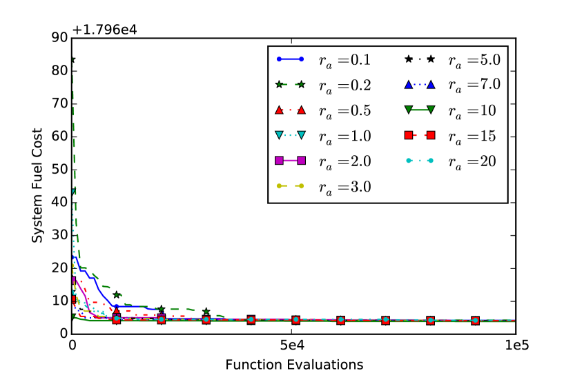
Figure 1: Convergence performance of SSA with different $r_{a}$ values.

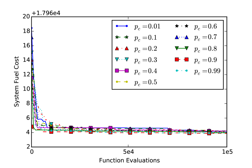
Figure 2: Convergence performance of SSA with different $p_{c}$ values.

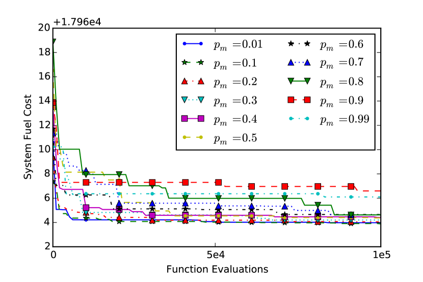
Figure 3: Convergence performance of SSA with different $p_{m}$ values.

6 Conclusion

In this paper we propose a new approach based on the social spider algorithm to solve the economic dispatch problem in power grid operation and control. Although the conventional ELD problem is convex and can be easily solved by mathematical programming methods, the power unit model it employs is not as precise as those considering more practical constraints, e.g., VPE, MFO, and POZ. These characteristics of power units make the optimization problem non-convex, non-differentiable, and non-continuous.

In order to efficiently solve the modern ELD problem, we propose a variant of SSA with new controlling schemes. A chaotic sequence based memory factor is introduced to control the searching pattern, where the previous movement of a spider in SSA is assigned with different degrees of importance with the process of optimization. In addition, we introduce a problem-specific power schedule repairing scheme to fix the infeasible solution generated in the random walk step. This repair scheme takes the power supper/demand and POZ constraints into account, while all other boundary constraints are handled by a boundary absorbing technique.

To evaluate the performance of our proposed SSA-based ELD solver, the approach is applied to solve five different test power systems with various numbers of power units and constraint configurations. The simulation results are compared with a wide range of the state-of-the-art algorithms in solving ELD within the employed test systems. SSA is able to find new best fuel cost solution in four out of the five systems, and can achieve the same solution quality in the remaining one. This result indicates the superiority of SSA in solving ELD with different configurations. In addition, we performed a parameter sensitivity test to develop a best performing combination of SSA parameters. The convergence performance of different parameter values are also presented for comparison. From all simulation results it can be concluded that our proposed SSA-based approach outperforms the existing state-of-the-art algorithms in solving non-convex ELD problems.

Appendix

Table 7: System Coefficients for 13-unit Test System with VPE

Unit($i$)	$P^{\textit{min}}_{i}$	$P^{\textit{max}}_{i}$	$a_{i}$	$b_{i}$	$c_{i}$	$e_{i}$	$f_{i}$
1	0	680	550	8.1	0.00028	300	0.035
2	0	360	309	8.1	0.00056	200	0.042
3	0	360	307	8.1	0.00056	200	0.042
4	60	180	240	7.74	0.00324	150	0.063
5	60	180	240	7.74	0.00324	150	0.063
6	60	180	240	7.74	0.00324	150	0.063
7	60	180	240	7.74	0.00324	150	0.063
8	60	180	240	7.74	0.00324	150	0.063
9	60	180	240	7.74	0.00324	150	0.063
10	40	120	126	8.6	0.00284	100	0.084
11	40	120	126	8.6	0.00284	100	0.084
12	55	120	126	8.6	0.00284	100	0.084
13	55	120	126	8.6	0.00284	100	0.084

Table 8: System Coefficients for 40-unit Test System with VPE

Unit($i$)	$P^{\textit{min}}_{i}$	$P^{\textit{max}}_{i}$	$a_{i}$	$b_{i}$	$c_{i}$	$e_{i}$	$f_{i}$	Unit($i$)	$P^{\textit{min}}_{i}$	$P^{\textit{max}}_{i}$	$a_{i}$	$b_{i}$	$c_{i}$	$e_{i}$	$f_{i}$
1	36	114	94.705	6.73	0.0069	100	0.084	21	254	550	785.96	6.63	0.00298	300	0.035
2	36	114	94.705	6.73	0.0069	100	0.084	22	254	550	785.96	6.63	0.00298	300	0.035
3	60	120	309.54	7.07	0.02028	100	0.084	23	254	550	794.53	6.66	0.00284	300	0.035
4	80	190	369.03	8.18	0.00942	150	0.063	24	254	550	794.53	6.66	0.00284	300	0.035
5	47	97	148.89	5.35	0.01140	120	0.077	25	254	550	801.32	7.10	0.00277	300	0.035
6	68	140	222.33	8.05	0.01142	100	0.084	26	254	550	801.32	7.10	0.00277	300	0.035
7	110	300	287.71	8.03	0.00357	200	0.042	27	10	150	1055.1	3.33	0.52124	120	0.077
8	135	300	391.98	6.99	0.00492	200	0.042	28	10	150	1055.1	3.33	0.52124	120	0.077
9	135	300	455.76	6.6	0.00573	200	0.042	29	10	150	1055.1	3.33	0.52124	120	0.077
10	130	300	722.82	12.9	0.00605	200	0.042	30	47	94	148.89	5.35	0.01140	120	0.077
11	94	375	635.20	12.9	0.00515	200	0.042	31	60	190	222.92	6.43	0.00160	150	0.063
12	94	375	654.69	12.8	0.00569	200	0.042	32	60	190	222.92	6.43	0.00160	150	0.063
13	125	500	913.40	12.5	0.00421	300	0.035	33	60	190	222.92	6.43	0.00160	150	0.063
14	125	500	1760.4	8.84	0.00752	300	0.035	34	90	200	107.87	8.95	0.00010	200	0.042
15	125	500	1728.3	9.15	0.00708	300	0.035	35	90	200	116.58	8.62	0.00010	200	0.042
16	125	500	1728.3	9.15	0.00708	300	0.035	36	90	200	116.58	8.62	0.00010	200	0.042
17	220	500	647.85	7.97	0.00313	300	0.035	37	25	110	307.45	5.88	0.01610	80	0.098
18	220	500	649.69	7.95	0.00313	300	0.035	38	25	110	307.45	5.88	0.01610	80	0.098
19	242	550	647.83	7.97	0.00313	300	0.035	39	25	110	307.45	5.88	0.01610	80	0.098
20	242	550	647.81	7.97	0.00313	300	0.035	40	242	550	647.83	7.97	0.00313	300	0.035

Table 9: System Coefficients for 10-unit Test System with VPE and MFO

Unit($i$)	Fuel($g$)	$P^{\textit{min}}_{i}$	$P^{\textit{max}}_{i}$	$a_{i}$	$b_{i}$	$c_{i}$	$e_{i}$	$f_{i}$
1	1	100	250	26.97	-0.3975	0.002176	0.02697	-3.9750
1	2	100	250	21.13	-0.3059	0.001861	0.02113	-3.0590
2	1	50	230	118.4	-1.2690	0.004194	0.11840	-12.690
2	2	50	230	1.865	-0.0399	0.001138	0.00187	-0.3988
2	3	50	230	13.65	-0.1980	0.001620	0.01365	-1.9800
3	1	200	500	39.79	-0.3116	0.001457	0.03979	-3.1160
3	2	200	500	-59.14	0.4864	0.00001176	-0.05914	4.8640
3	3	200	500	-2.876	0.0339	0.0008035	-0.00288	0.3389
4	1	99	265	1.983	-0.0311	0.001049	0.00198	-0.3114
4	2	99	265	52.85	-0.6348	0.002758	0.05285	-6.3480
4	3	99	265	266.8	-2.3380	0.005935	0.26680	-23.380
5	1	190	490	13.92	-0.0873	0.001066	0.01392	-0.8733
5	2	190	490	99.76	-0.5206	0.001597	0.09976	-5.2060
5	3	190	490	-53.99	0.4462	0.0001498	-0.05399	4.4620
6	1	85	265	52.15	-0.6348	0.002758	0.05285	-6.3480
6	2	85	265	1.983	-0.0311	0.001049	0.00198	-0.3114
6	3	85	265	266.6	-2.3380	0.005935	0.26680	-23.380
7	1	200	500	18.93	-0.1325	0.001107	0.01893	-1.3250
7	2	200	500	43.77	-0.2267	0.001165	0.04377	-2.2670
7	3	200	500	43.35	0.3559	0.0002454	-0.04335	3.5590
8	1	99	265	1.983	-0.0311	0.001049	0.00198	-0.3114
8	2	99	265	52.85	-0.6348	0.002758	0.05285	-6.3480
8	3	99	265	266.8	-2.3380	0.005935	0.26680	-23.380
9	1	130	440	88.53	-0.5675	0.001554	0.08853	-5.6750
9	2	130	440	15.32	-0.0451	0.007033	0.01423	-0.1817
9	3	130	440	14.23	-0.0182	0.0006121	0.01423	-0.1817
10	1	200	490	13.97	-0.0994	0.001102	0.01397	-0.9938
10	2	200	490	-61.13	0.5084	0.00004164	-0.06113	5.0840
10	3	200	490	46.71	-0.2024	0.001137	0.04671	-2.0240

Table 10: System Coefficients for 6-unit Test System with POZ and Line Loss

Unit($i$)	$P^{\textit{min}}_{i}$	$P^{\textit{max}}_{i}$	$a_{i}$	$b_{i}$	$c_{i}$	$P^{\textit{UR}}$	$P^{\textit{DR}}$	$P^{\textit{prev}}_{i}$	POZs
1	100	500	240	7.0	0.0070	80	120	440	$[210,240],[350,380]$
2	50	200	200	10.0	0.0095	50	90	170	$[90,110],[140,160]$
3	80	300	220	8.5	0.0090	65	100	200	$[150,170],[210,240]$
4	50	150	200	11.0	0.0090	50	90	150	$[80,90],[110,120]$
5	50	200	220	10.5	0.0080	50	90	190	$[90,110],[140,150]$
6	50	120	190	12.0	0.0075	50	90	110	$[75,85],[100,105]$

Table 11: System Coefficients for 15-unit Test System with POZ and Line Loss

Unit($i$)	$P^{\textit{min}}_{i}$	$P^{\textit{max}}_{i}$	$a_{i}$	$b_{i}$	$c_{i}$	$P^{\textit{UR}}$	$P^{\textit{DR}}$	$P^{\textit{prev}}_{i}$	POZs
1	150	455	671	10.1	0.000299	80	120	400
2	150	455	574	10.2	0.000183	80	120	300	$[185,225],[305,335],[420,450]$
3	20	130	374	8.80	0.001126	130	130	105
4	20	130	374	8.80	0.001126	130	130	100
5	150	470	461	10.4	0.000205	80	120	90	$[180,200],[305,335],[390,420]$
6	135	460	630	10.1	0.000301	80	120	400	$[230,255],[365,395],[430,455]$
7	135	465	548	9.80	0.000364	80	120	350
8	60	300	227	11.2	0.000338	65	100	95
9	25	162	173	11.2	0.000807	60	100	105
10	25	160	175	10.7	0.001203	60	100	110
11	20	80	186	10.2	0.003586	80	80	60
12	20	80	230	9.90	0.005513	80	80	40	$[30,40],[55,65]$
13	25	85	225	13.1	0.000371	80	80	30
14	15	55	309	12.1	0.001929	55	55	20
15	15	55	323	12.4	0.004447	55	55	20

The system coefficients and configurations are presented in Tables 7, 8, 9, 10, and 11.

References

References

- [1] A. J. Wood, B. F. Wollenberg, Power Generation, Operation and Control, John Wiley & Sons Inc, New York, NY, USA, 1984.
- [2] J. Dodu, P. Martin, A. Merlin, J. Pouget, An optimal formulation and solution of short-range operating problems for a power system with flow constraints, Proceedings of the IEEE 60 (1) (1972) 54–63.
- [3] C.-L. Chen, S. Wang, Branch-and-bound scheduling for thermal generating units, IEEE Trans. on Energy Conversion 8 (2) (1993) 184–189.
- [4] J.-Y. Fan, L. Zhang, Real-time economic dispatch with line flow and emission constraints using quadratic programming, IEEE Trans. on Power Systems 13 (2) (1998) 320–325.
- [5] J. J. Q. Yu, V. O. K. Li, A. Y. S. Lam, Optimal V2G scheduling of electric vehicles and unit commitment using chemical reaction optimization, in: Proc. IEEE Congress on Evolutionary Computation (CEC), Cancun, Mexico, 2013, pp. 392–399.
- [6] R.-M. Jan, N. Chen, Application of the fast newton-raphson economic dispatch and reactive power/voltage dispatch by sensitivity factors to optimal power flow, IEEE Trans. on Energy Conversion 10 (2) (1995) 293–301.
- [7] W.-M. Lin, F.-S. Cheng, M.-T. Tsay, An improved tabu search for economic dispatch with multiple minima, IEEE Trans. on Power Systems 17 (1) (2002) 108–112.
- [8] D. Liu, Y. Cai, Taguchi method for solving the economic dispatch problem with nonsmooth cost functions, IEEE Trans. on Power Systems 20 (4) (2005) 2006–2014.
- [9] Z.-L. Gaing, Particle swarm optimization to solving the economic dispatch considering the generator constraints, IEEE Trans. on Power Systems 18 (3) (2003) 1187–1195.
- [10] J.-B. Park, Y.-W. Jeong, J.-R. Shin, K. Y. Lee, An improved particle swarm optimization for nonconvex economic dispatch problems, IEEE Trans. on Power Systems 25 (1) (2010) 156–166.
- [11] J. Zhan, Q. H. Wu, C. Guo, X. Zhou, Economic dispatch with non-smooth objectives - Part II: Dimensional steepest decline method, IEEE Trans. on Power Systems 30 (2) (2015) 722–733.
- [12] J. J. Q. Yu, V. O. K. Li, A social spider algorithm for global optimization, Appl. Soft Comput. 30 (2015) 614–627.
- [13] C. W. Clark, M. Mangel, Foraging and flocking strategies: Information in an uncertain environment, The American Naturalist 123 (5) (1984) 626–641.
- [14] G. Uetz, Foraging strategies of spiders, Trends in Ecology and Evolution 7 (5) (1992) 155–159.
- [15] J. J. Q. Yu, V. O. K. Li, Base station switching problem for green cellular networks with social spider algorithm, in: Proc. IEEE Congress on Evolutionary Computation (CEC), Beijing, China, 2014, pp. 1–7.
- [16] C. Lin, G. Viviani, Hierarchical economic dispatch for piecewise quadratic cost functions, IEEE Trans. on Power Apparatus and Systems PAS-103 (6) (1984) 1170–1175.
- [17] J. Park, Y. Kim, I. Eom, K. Lee, Economic load dispatch for piecewise quadratic cost function using hopfield neural network, IEEE Trans. on Power Systems 8 (3) (1993) 1030–1038.
- [18] K. Lee, A. Sode-Yome, J. H. Park, Adaptive hopfield neural networks for economic load dispatch, IEEE Trans. on Power Systems 13 (2) (1998) 519–526.
- [19] F. Lee, A. Breipohl, Reserve constrained economic dispatch with prohibited operating zones, IEEE Trans. on Power Systems 8 (1) (1993) 246–254.
- [20] G. Binetti, A. Davoudi, D. Naso, B. Turchiano, F. Lewis, A distributed auction-based algorithm for the nonconvex economic dispatch problem, IEEE Transactions on Industrial Informatics 10 (2) (2014) 1124–1132.
- [21] S. Orero, M. Irving, Economic dispatch of generators with prohibited operating zones: a genetic algorithm approach, IEE Proceedings on Generation, Transmission and Distribution 143 (6) (1996) 1350–1260.
- [22] C.-L. Chiang, Improved genetic algorithm for power economic dispatch of units with valve-point effects and multiple fuels, IEEE Trans. on Power Systems 20 (4) (2005) 1690–1699.
- [23] D. He, F. Wang, Z. Mao, A hybrid genetic algorithm approach based on differential evolution for economic dispatch with valve-point effect, International Journal of Electrical Power & Energy Systems 30 (1) (2008) 31–38.
- [24] N. Sinha, R. Chakrabarti, P. Chattopadhyay, Evolutionary programming techniques for economic load dispatch, IEEE Transactions on Evolutionary Computation 7 (1) (2003) 83–94.
- [25] A. Pereira-Neto, C. Unsihuay, O. Saavedra, Efficient evolutionary strategy optimisation procedure to solve the nonconvex economic dispatch problem with generator constraints, IEE Proceedings on Generation, Transmission and Distribution 152 (5) (2005) 653–660.
- [26] S.-K. Wang, J.-P. Chiou, C. Liu, Non-smooth/non-convex economic dispatch by a novel hybrid differential evolution algorithm, IET Generation, Transmission and Distribution 1 (5) (2007) 793–803.
- [27] N. Nomana, H. Iba, Differential evolution for economic load dispatch problems, Electric Power Systems Research 78 (8) (2008) 1322–1331.
- [28] A. Selvakumar, K. Thanushkodi, A new particle swarm optimization solution to nonconvex economic dispatch problems, IEEE Trans. on Power Systems 22 (1) (2007) 42–51.
- [29] A. I. Selvakumara, K. Thanushkodi, Anti-predatory particle swarm optimization: Solution to nonconvex economic dispatch problems, Electric Power Systems Research 78 (1) (2008) 2–10.
- [30] K. Chaturvedi, Gwalior, M. Pandit, L. Srivastava, Self-organizing hierarchical particle swarm optimization for nonconvex economic dispatch, IEEE Trans. on Power Systems 23 (3) (2008) 1079–1087.
- [31] K. Meng, H. G. Wang, Z. Dong, K. P. Wong, Quantum-inspired particle swarm optimization for valve-point economic load dispatch, IEEE Trans. on Power Systems 25 (1) (2010) 215–222.
- [32] A. Safaria, H. Shayeghi, Iteration particle swarm optimization procedure for economic load dispatch with generator constraints, Expert Systems with Applications 38 (5) (2011) 6043–6048.
- [33] R. Kumara, A. Sadua, R. Kumara, S. Panda, A novel multi-objective directed bee colony optimization algorithm for multi-objective emission constrained economic power dispatch, International Journal of Electrical Power & Energy Systems 43 (1) (2012) 1241–1250.
- [34] A. Bhattacharya, P. Chattopadhyay, Biogeography-based optimization for different economic load dispatch problems, IEEE Transactions on Power Systems 25 (2) (2010) 1064–1077.
- [35] J. Cai, Q. Li, L. Li, H. Peng, Y. Yang, A fuzzy adaptive chaotic ant swarm optimization for economic dispatch, International Journal of Electrical Power & Energy Systems 34 (1) (2012) 156–160.
- [36] L. dos Santos Coelho, V. C. Mariani, An improved harmony search algorithm for power economic load dispatch, Energy Conversion and Management 50 (10) (2009) 2522–2526.
- [37] P. K. Roy, S. Bhui, C. Paul, Solution of economic load dispatch using hybrid chemical reaction optimization approach, Appl. Soft Comput. 24 (2014) 109–125.
- [38] E. Araujo, L. dos S. Coelho, Particle swarm approaches using lozi map chaotic sequences to fuzzy modelling of an experimental thermal-vacuum system, Appl. Soft Comput. 8 (4) (2008) 1354–1364.
- [39] R. Caponetto, L. Fortuna, S. Fazzino, M. Xibilia, Chaotic sequences to improve the performance of evolutionary algorithms, IEEE Trans. Evol. Comput. 7 (3) (2003) 289–304.
- [40] J. J. Q. Yu, V. O. K. Li, Parameter sensitivity analysis of social spider algorithm, in: Proc. IEEE Congress on Evolutionary Computation (CEC), Sendai, Japan, 2015, accepted for publication.
- [41] W. Chu, X. Gao, S. Sorooshian, Handling boundary constraints for particle swarm optimization in high-dimensional search space, Inform. Sci. 181 (20) (2011) 4569–4581.
- [42] T. Niknam, H. D. Mojarrad, H. Z. Meymand, A novel hybrid particle swarm optimization for economic dispatch with valve-point loading effects, Energy Conversion and Management 52 (4) (2011) 1800–1809.
- [43] H. Lu, P. Sriyanyong, Y. H. Song, T. Dillon, Experimental study of a new hybrid pso with mutation for economic dispatch with non-smooth cost function, International Journal of Electrical Power & Energy Systems 32 (9) (2010) 921–935.
- [44] B. Panigrahi, V. R. Pandi, Bacterial foraging optimisation: Nelder cmead hybrid algorithm for economic load dispatch, IET Generation, Transmission & Distribution 2 (4) (2008) 556–565.
- [45] X.-S. Yang, S. S. S. Hosseini, A. H. Gandomi, Firefly algorithm for solving non-convex economic dispatch problems with valve loading effect, Appl. Soft Comput. 12 (3) (2012) 1180–1186.