Complex-mass renormalization in hadronic EFT:
applicability at two-loop order

Abstract

We discuss the application of the complex-mass scheme to multi-loop diagrams in hadronic effective field theory by considering as an example a two-loop self-energy diagram. We show that the renormalized two-loop diagram satisfies the power counting.

I Introduction

The extension of mesonic chiral perturbation theory Weinberg:1979kz ; Gasser:1984gg ; Gasser:1984yg to include heavier (non-Goldstone) degrees of freedom is known to be a non-trivial problem. Already in the one-nucleon sector it was found that higher-order loops contribute to lower-order calculations Gasser:1988rb . This problem, also for the delta resonance included as a dynamical degree of freedom, has been solved in the framework of the heavy-baryon chiral perturbation theory Jenkins:1991jv ; Bernard:1992qa ; Hemmert:1996xg and later in the original manifestly Lorentz-invariant formulations by using the infrared regularization and the extended on-mass-shell renormalization (EOMS) Tang:1996ca ; Ellis:1997kc ; Becher:1999he ; Gegelia:1999gf ; Gegelia:1999qt ; Fuchs:2003qc . It is also possible to consistently include virtual (axial-) vector mesons in effective field theory (EFT) Kubis:2000zd ; Fuchs:2003sh ; Schindler:2003xv for processes involving soft external pions and nucleons with small three-momenta. On the other hand, as the (axial-) vector mesons decay into light modes (and therefore large imaginary parts appear), the issue of including (axial-) vector mesons in an EFT for energies when the intermediate resonant states can be generated is still very problematic Bruns:2004tj . First attempts have been made to handle this problem by applying the complex mass scheme Stuart:1990 ; Denner:1999gp in Refs. Djukanovic:2009zn ; Djukanovic:2009gt ; Djukanovic:2010id ; Bauer:2011bv ; Bauer:2012at ; Djukanovic:2013mka .

The aim of this work is to explicitly demonstrate the applicability of the complex-mass scheme to multi-loop diagrams. For that we analyze a two-loop self-energy diagram within the complex-mass scheme, similar to what was done in Ref. Schindler:2003je using the infrared regularization and the EOMS renormalization. We show that the resulting renormalized expressions for the two-loop diagram indeed satisfy the power counting of the considered EFT.

II A two-loop $\omega$-meson self-energy diagram

We start with a two-loop self-energy diagram of the $\omega$-meson shown in Fig. 1 a), where the solid lines correspond to the vector meson and the dashed ones to the pion. This diagram is generated by the interaction Lagrangian Meissner:1987ge :

$${\cal L}_{V\Phi\Phi\Phi}^{(1)}=\frac{i\,h}{4F_{\pi}^{3}}\,\epsilon^{\mu\nu\alpha\beta}\,{\rm tr}\left(V_{\mu}\partial_{\nu}\Phi\partial_{\alpha}\Phi\partial_{\beta}\Phi\right),$$ (1)

where $V_{\mu}$ is the vector field corresponding to the $\omega$ meson and $\Phi=\pi^{a}\tau^{a}$ to the pions (for the case of the two-flavor chiral effective field theory, which we consider here).

Calculating the diagram of Fig. 1 a) we obtain:

$$i\,\Sigma^{\mu\nu}=\frac{9\,ih^{2}}{F_{\pi}^{6}}\,\epsilon^{\mu\lambda_{1}\sigma_{1}\kappa_{1}}\,\epsilon^{\nu\lambda_{2}\sigma_{2}\kappa_{2}}\,p_{\kappa_{1}}p_{\kappa_{2}}I_{\lambda_{1}\sigma_{1}\lambda_{2}\sigma_{2}},$$ (2)

where

$$I^{\lambda_{1}\sigma_{1}\lambda_{2}\sigma_{2}}=\frac{1}{(2\pi)^{2n}}\int\frac{d^{n}k_{1}d^{n}k_{2}\,k_{1}^{\lambda_{1}}k_{1}^{\lambda_{2}}k_{2}^{\sigma_{1}}k_{2}^{\sigma_{2}}}{\left[k_{1}^{2}-M^{2}+i0^{+}\right]\left[k_{2}^{2}-M^{2}+i0^{+}\right]\left[(p+k_{1}+k_{2})^{2}-M^{2}+i0^{+}\right]}.$$ (3)

Using the tensor integral reduction formulas specified in the Appendix C of Ref. Schindler:2007dr and simplifying Eq. (2) we obtain

$$i\,\Sigma^{\mu\nu}=\frac{72\,i\pi^{2}h^{2}}{F_{\pi}^{6}}\,\left(p^{\mu}p^{\nu}-p^{2}g^{\mu\nu}\right)I_{n+2},$$ (4)

where

$$I_{n+2}=\frac{1}{(2\pi)^{2(n+2)}}\int\frac{d^{n+2}k_{1}d^{n+2}k_{2}}{\left[k_{1}^{2}-M^{2}+i0^{+}\right]\left[k_{2}^{2}-M^{2}+i0^{+}\right]\left[(p+k_{1}+k_{2})^{2}-M^{2}+i0^{+}\right]}.$$ (5)

Thus the investigation of the considered two-loop diagram contributing to the $\omega$-meson self-energy reduces to the study of a scalar integral in 6 dimensions.

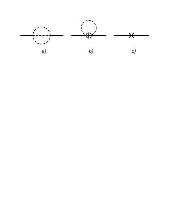
Figure 1: Two-loop order self-energy diagrams. The vertex with a circled cross corresponds to a one-loop order counterterm and a mere cross corresponds to two-loop order counterterms. Solid/dashed lines correspond to heavy/light particles.

III Lagrangian and power counting

To properly subtract the two-loop integral of the previous section by applying the complex mass scheme without unnecessary complications due to the spin and chiral structure of the low-energy effective field theory, we focus here on an effective field theoretical model Lagrangian of interacting scalar fields in six space-time dimensions

$$\mathcal{L}=\frac{1}{2}(\partial_{\mu}\pi\partial^{\mu}\pi-M^{2}\pi^{2})+\frac{1}{2}(\partial_{\mu}\Psi\partial^{\mu}\Psi-m^{2}\Psi^{2})-\frac{g}{3!}\,\pi^{3}\Psi+\mathcal{L}_{1}~{},$$ (6)

where the masses of the scalar fields $\pi$ and $\Psi$ satisfy the condition $M\ll m$ (i.e. $\Psi$ represents an unstable particle). The Lagrangian $\mathcal{L}_{1}$ contains all possible terms which are consistent with the Lorentz symmetry and with the invariance under the simultaneous transformations $\pi\to-\pi$ and $\Psi\to-\Psi$. Within the considered EFT, we drop heavy-particle loops, however, we compensate for their contributions by including them in the low-energy constants. The application of the complex-mass scheme guarantees that subtracted Feynman diagrams have a certain “chiral” order $D$, specified by the power counting. In particular, let $Q$ stand for small quantities like the mass $M$, small external four-momenta of $\pi$ or small external three-momenta of $\Psi$. Then the vertex generated by the $\pi\Psi$ interaction explicitly shown in Eq. (6) counts as $Q^{0}$, the $\Psi$ propagator as $Q^{-1}$, the $\pi$ propagator as $Q^{-2}$, and a loop integration in $n$ dimensions as $Q^{n}$, respectively.

IV Application to the two-loop self-energy

Here we consider the $\Psi$ self-energy diagram shown in Fig. 1  a). The corresponding expression reads:

$$-i\Sigma_{\Psi}(p)=\frac{i\,g^{2}}{6(2\pi)^{2n}}\int\int\frac{d^{n}k_{1}d^{n}k_{2}}{(k_{1}^{2}-M^{2}+i0^{+})(k_{2}^{2}-M^{2}+i0^{+})[(p+k_{1}+k_{2})^{2}-M^{2}+i0^{+}]}~{},$$ (7)

where $1/6$ is a symmetry factor and $n$ denotes the number of space-time dimensions. According to the above power counting, the diagram of Fig. 1 a) has the order $Q^{2n-4}$.

Using the dimensional counting analysis of Ref. Gegelia:zz (or equivalently, the ”strategy of regions” Beneke:1997zp ), the self-energy $\Sigma_{\Psi}$ for $M\to 0$ and $p^{2}\sim m^{2}$ can be written as

$$\Sigma_{\Psi}=F(p^{2},M^{2},n)+M^{n-2}G(p^{2},M^{2},n)+M^{2n-4}H(p^{2},M^{2},n)~{},$$ (8)

where the functions $F(p^{2},M^{2},n)$, $G(p^{2},M^{2},n)$, and $H(p^{2},M^{2},n)$ can be expanded in non-negative integer powers of $M^{2}$. The coefficients of the Taylor expansion of $F$ in $M^{2}$ can be obtained by expanding the integrand of Eq. (7) in $M^{2}$ and interchanging summation and integration:

$$F(p^{2},M^{2},n)=-\frac{g^{2}}{6}\sum_{i,j,l=0}^{\infty}\frac{(M^{2})^{i+j+l}}{(2\pi)^{2n}}\int\int\frac{d^{n}k_{1}d^{n}k_{2}}{(k_{1}^{2}+i0^{+})^{1+i}(k_{2}^{2}+i0^{+})^{1+j}[(p+k_{1}+k_{2})^{2}+i0^{+}]^{1+\,l}}~{}.$$ (9)

Calculating the integrals of Eq. (9) we obtain

$$\int\int\frac{d^{n}k_{1}d^{n}k_{2}}{(k_{1}^{2}+i0^{+})^{1+i}(k_{2}^{2}+i0^{+})^{1+j}[(p+k_{1}+k_{2})^{2}+i0^{+}]^{1+\,l}}=\pi^{n}i^{-2(i+j+l)}\left(-p^{2}-i0^{+}\right)^{n-i-j-l-3}$$

$$\times\frac{\Gamma\left(\frac{n}{2}-i-1\right)\Gamma\left(\frac{n}{2}-j-1\right)\Gamma\left(\frac{n}{2}-l-1\right)\Gamma(i+j+l-n+3)}{\Gamma(i+1)\Gamma(j+1)\Gamma(l+1)\Gamma\left(\frac{3n}{2}-i-j-l-3\right)}~{}.$$ (10)

The terms in Eq. (9) are analytic in $M^{2}$. In order to find the power counting violating terms, we need to expand the coefficients of the series in Eq. (9) in terms of $p^{2}-m^{2}$. We only need to subtract those terms which violate the power counting, which in the present case of six space-time dimensions are all terms of order $Q^{7}$ or less. Doing so we identify the subtraction terms which are analytic in $M^{2}$ and $p^{2}-M^{2}$. These subtraction terms are canceled by counterterm contributions, shown in Fig. 1 c). As is clear from Eq. (IV), the counterterms have to be complex.

Next we investigate $G(p^{2},M^{2},n)$ which can be found from Eq. (7) as a sum of terms identified by re-scaling ($k_{1}\mapsto Mk_{1},k_{2}\mapsto k_{2}$), ($k_{1}\mapsto k_{1},k_{2}\mapsto Mk_{2}$) and ($k_{1}\mapsto Mk_{1}-k_{2}-p,k_{2}\mapsto k_{2}$). In all cases, the re-scaling generates an overall factor of $M^{n-2}$. The remaining integrands need to be expanded in $M$, the summation and integration interchanged. Doing the above manipulations and adding all terms together we obtain

$$G(p^{2},M^{2},n)=-\frac{g^{2}}{2\,(2\pi)^{2n}}\sum_{i,j=0}^{\infty}\sum_{a=0}^{j}\sum_{b=0}^{a}(-1)^{j}2^{j-b}\left(\begin{array}[]{c}j\\ a\end{array}\right)\left(\begin{array}[]{c}a\\ b\end{array}\right)M^{2i+j+b}I_{ij,ab}(p^{2},n)~{},$$ (11)

with the binomial coefficients

$$\left(\begin{array}[]{c}r\\ s\end{array}\right)=\frac{r!}{s!(r-s)!}~{},$$

and the integrals $I_{ij,ab}(p^{2},n)$ given as

$$I_{ij,ab}(p^{2},n)=\int\int\frac{d^{n}k_{1}d^{n}k_{2}\,(p\cdot k_{1})^{j-a}(k_{1}\cdot k_{2})^{a-b}(k_{1}^{2}-1)^{b}}{(k_{1}^{2}-1+i0^{+}){(k_{2}^{2}+i0^{+})}^{1+i}{[(p+k_{2})^{2}+i0^{+}]}^{1+j}}~{}.$$ (12)

The non-vanishing terms in Eq. (11) contain only nonnegative integer powers of $M^{2}$. This is because for $j+b$ odd, the loop integral of Eq. (12) is an odd function of $k_{1}$ and hence vanishes.

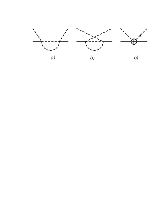
Figure 2: One-loop diagrams contributing to $\pi\Psi$ scattering.

The only power counting violating contributions are contained in the terms of Eq. (11) with $2i+j+b$ equal to either $0$ or $2$. Calculating these contributions we obtain:

$$M^{n-2}\Delta G = \frac{g^{2}M^{n-2}\left(-m^{2}-i0^{+}\right)^{\frac{n}{2}-5}}{96(4\pi)^{n}}\Gamma\left(1-\frac{n}{2}\right)\Gamma\left(2-\frac{n}{2}\right)\Gamma\left(\frac{n}{2}-1\right)^{2}\Biggl{\{}\frac{48\,m^{6}}{\Gamma(n-2)}$$ (13)

$$+ 6m^{2}\left[\frac{\left(m^{2}-p^{2}\right)^{2}\left(n-4\right)(n-6)}{\Gamma(n-2)}-\frac{8m^{2}M^{2}(n+4)}{n\Gamma(n-3)}\right]-\frac{24m^{4}\left(m^{2}-p^{2}\right)\left(n-4\right)}{\Gamma(n-2)}$$

$$- (n-6)\left(m^{2}-p^{2}\right)\left(\frac{\left(m^{2}-p^{2}\right)^{2}\left(n-4\right)(n-8)}{\Gamma(n-2)}-\frac{24m^{2}M^{2}(n+4)}{n\Gamma(n-3)}\right)\Biggr{\}}.$$

These terms are canceled by the diagram shown in Fig. 1 b). The one-loop counterterms contributing in this diagram originate from the one-loop diagrams of Fig. 2 a) and b). Expressions corresponding to these diagrams are given by

$$\mathcal{M}_{2a}=\frac{g^{2}}{2}\int\frac{d^{n}k}{(2\pi)^{n}}\frac{1}{(k^{2}-M^{2}+i0^{+})[(k+p+q)^{2}-M^{2}+i0^{+}]}~{},$$ (14)

and

$$\mathcal{M}_{2b}=\frac{g^{2}}{2}\int\frac{d^{n}k}{(2\pi)^{n}}\frac{1}{(k^{2}-M^{2}+i0^{+})[(k+p-q^{\prime})^{2}-M^{2}+i0^{+}]}~{},$$ (15)

respectively.

The diagrams in Fig. 2 a) and b) are of the order $Q^{n-2}$. Loop integrals in Eqs. (14) and (15) contain contributions that violate the power counting, namely:

$$\Delta\mathcal{M}_{2a}+\Delta\mathcal{M}_{2b} = \frac{ig^{2}\lambda(m,n)}{48m^{6}(n-4)}\biggl{\{}2m^{6}(n-10)(n-8)(n-6)$$

$$- 3m^{4}(n-8)\left(32M^{2}(n-3)+(n-10)(n-4)\left[(p-q^{\prime})^{2}+(p+q)^{2}\right]\right)$$

$$+ 3m^{2}(n-6)\biggl{[}16M^{2}(n-3)\left[(p-q^{\prime})^{2}+(p+q)^{2}\right]$$

$$+ (n-10)(n-4)\left(\left((p-q^{\prime})^{2}\right)^{2}+\left((p+q)^{2}\right)^{2}\right)\biggr{]}$$

$$- (n-8)(n-6)(n-4)\left[\left((p-q^{\prime})^{2}\right)^{3}+\left((p+q)^{2}\right)^{3}\right]\biggr{\}},$$

$$\lambda(m,n) = \frac{\Gamma\left(3-\frac{n}{2}\right)\Gamma\left(\frac{n}{2}-1\right)^{2}}{(4\pi)^{n/2}\Gamma(n-2)}\left(-\frac{m^{2}+i0^{+}}{\mu^{2}}\right)^{n/2-2}~{}.$$ (16)

The counterterm diagram which cancels these contributions is shown in Fig. 2 c) and is generated by a rather complicated Lagrangian which is contained in the ${\cal L}_{1}$ term of Eq. (6).

When calculating the self-energy of $\Psi$, these counterterms give a contribution shown in Fig. 1 b). The corresponding expression reads

$$-i\Sigma_{CT} = -\frac{ig^{2}\lambda(m,n)}{48m^{6}(n-4)n}\Biggl{\{}m^{6}(n-10)(n-8)(n-6)n$$ (17)

$$- 3m^{4}(n-8)n\left[M^{2}(n-2)(n+4)+(n-10)(n-4)p^{2}\right]$$

$$+ 3m^{2}(n-6)\biggl{[}M^{4}(n-2)n(n+4)$$

$$+ 2M^{2}(n+4)((n-8)n+20)p^{2}+(n-10)(n-4)np^{4}\biggr{]}$$

$$- (n-8)(n-6)(n-4)\left(M^{2}+p^{2}\right)\left(M^{4}n+2M^{2}(n+6)p^{2}+np^{4}\right)\Biggr{\}}I_{\pi},$$

where

$$I_{\pi}=i\int\frac{d^{n}k}{(2\pi)^{n}}\frac{1}{k^{2}-M^{2}+i0^{+}}=M^{n-2}\frac{\Gamma(1-n/2)}{(4\pi)^{n/2}}~{}.$$ (18)

Indeed, as already mentioned above, the self-energy contribution of Eq. (17) cancels the power counting violating contributions in Eq. (13).

Finally, the function $H(p^{2},M^{2},n)$ is given as a sum of three terms obtained from Eq. (7) by re-scalings ($k_{1}\mapsto Mk_{1}$, $k_{2}\mapsto Mk_{2}$), ($k_{1}\mapsto Mk_{1}-p$, $k_{2}\mapsto Mk_{2}$) and ($k_{1}\mapsto Mk_{1}$, $k_{2}\mapsto Mk_{2}-p$), extracting a factor of $M^{2n-4}$, expanding the remaining integrand in $M$, and interchanging integration and summation, yielding

$$H(p^{2},M^{2},n) = -\frac{g^{2}}{2(2\pi)^{2n}}\frac{1}{p^{2}}\sum_{i=0}^{\infty}(-1)^{i}\left(\frac{M}{p^{2}}\right)^{i}$$ (21)

$$\times\sum_{j=0}^{i}\left(\begin{array}[]{c}i\\ j\end{array}\right)\int\int d^{n}k_{1}d^{n}k_{2}\frac{[2p\cdot(k_{1}+k_{2})]^{i-j}[M(k_{1}+k_{2})^{2}-M]^{j}}{(k_{1}^{2}-1+i0^{+})(k_{2}^{2}-1+i0^{+})}~{}.$$

It is easy to see that Eq. (21), in combination with the factor $M^{2n-4}$ of Eq. (8), satisfies the power counting.

Combining the results above, we conclude that all terms violating the power counting are canceled in the sum of diagrams shown in Fig. 1.

V Conclusion

In conclusion, using as example a two-loop self-energy diagram in an EFT of interacting light and heavy scalar particles we have demonstrated that the application of the complex-mass scheme to two-loop diagrams leads to a consistent power counting. As expected from general considerations, the subtraction of one-loop sub-diagrams plays an important role in the renormalization of the two-loop diagrams. Our example provides an explicit illustration of the fact that the application of the complex-mass scheme to multi-loop diagrams of a low-energy effective field theory leads to a consistent power counting. Calculations using the chiral effective Lagrangians are more involved due to the complicated structure of the interactions, but the general features of the renormalization program do not change. As we have shown, such a typical heavy-light two-loop self-energy diagram emerges naturally when considering a chiral EFT with $\omega$-mesons and pions.

References

• (1) S. Weinberg, Physica A 96, 327 (1979).
• (2) J. Gasser and H. Leutwyler, Ann. Phys.  (N.Y.) 158, 142 (1984).
• (3) J. Gasser and H. Leutwyler, Nucl. Phys. B250, 465 (1985).
• (4) J. Gasser, M. E. Sainio, and A. Švarc, Nucl. Phys. B307, 779 (1988).
• (5) E. Jenkins and A. V. Manohar, Phys. Lett. B 255, 558 (1991).
• (6) V. Bernard, N. Kaiser, J. Kambor, and U.-G. Meißner, Nucl. Phys. B388, 315 (1992).
• (7) T. R. Hemmert, B. R. Holstein and J. Kambor, Phys. Lett. B 395, 89 (1997).
• (8) H. Tang, hep-ph/9607436.
• (9) P. J. Ellis and H. Tang, Phys. Rev. C 57, 3356 (1998).
• (10) T. Becher and H. Leutwyler, Eur. Phys. J. C 9, 643 (1999).
• (11) J. Gegelia and G. Japaridze, Phys. Rev. D 60, 114038 (1999).
• (12) J. Gegelia, G. Japaridze, and X. Q. Wang, J. Phys. G 29, 2303 (2003).
• (13) T. Fuchs, J. Gegelia, G. Japaridze, and S. Scherer, Phys. Rev. D 68, 056005 (2003).
• (14) T. Fuchs, M. R. Schindler, J. Gegelia, and S. Scherer, Phys. Lett. B 575, 11 (2003).
• (15) B. Kubis and U.-G. Meißner, Nucl. Phys. A 679, 698 (2001).
• (16) M. R. Schindler, J. Gegelia, and S. Scherer, Phys. Lett.  B 586, 258 (2004).
• (17) P. C. Bruns and U.-G. Meißner, Eur. Phys. J. C 40, 97 (2005).
• (18) R. G. Stuart, in ${\rm Z}^{0}$ Physics, ed. J. Tran Thanh Van (Editions Frontieres, Gif-sur-Yvette, 1990), p.41.
• (19) A. Denner, S. Dittmaier, M. Roth and D. Wackeroth, Nucl. Phys.  B560, 33 (1999).
• (20) D. Djukanovic, J. Gegelia, A. Keller and S. Scherer, Phys. Lett. B 680, 235 (2009).
• (21) D. Djukanovic, J. Gegelia and S. Scherer, Phys. Lett. B 690, 123 (2010).
• (22) D. Djukanovic, J. Gegelia, A. Keller and S. Scherer, PoS CD 09, 050 (2009).
• (23) T. Bauer, D. Djukanovic, J. Gegelia, S. Scherer and L. Tiator, AIP Conf. Proc.  1432, 269 (2012).
• (24) T. Bauer, J. Gegelia and S. Scherer, Phys. Lett. B 715, 234 (2012).
• (25) D. Djukanovic, E. Epelbaum, J. Gegelia and U.-G. Meißner, Phys. Lett. B 730, 115 (2014).
• (26) T. Bauer, J. Gegelia, G. Japaridze and S. Scherer, Int. J. Mod. Phys. A 27, 1250178 (2012).
• (27) A. Denner and J. N. Lang, arXiv:1406.6280 [hep-ph].
• (28) M. R. Schindler, J. Gegelia and S. Scherer, Nucl. Phys. B 682, 367 (2004).
• (29) U.-G. Meißner, Phys. Rept.  161, 213 (1988).
• (30) M. R. Schindler, D. Djukanovic, J. Gegelia and S. Scherer, Nucl. Phys. A 803, 68 (2008).
• (31) J. Gegelia, G. S. Japaridze, and K. S. Turashvili, Theor. Math. Phys.  101, 1313 (1994) [Teor. Mat. Fiz. 101, 225 (1994)].
• (32) M. Beneke and V. A. Smirnov, Nucl. Phys. B 522, 321 (1998).