The behavior of the heavy-quarks structure functions at small-$x$

Abstract

The behavior of the charm and bottom structure functions ($F_{k}^{i}(x,Q^{2})$, i=c,b; k=2,L) at small-$x$ is considered with respect to the hard-Pomeron and saturation models. Having checked that this behavior predicate the heavy flavor reduced cross sections concerning the unshadowed and shadowed corrections. We will show that the effective exponents for the unshadowed and saturation corrections are independent of $x$ and $Q^{2}$, and also the effective coefficients are dependent to $\ln{Q^{2}}$ compared to Donnachie-Landshoff (DL) and color dipole (CD) models.

1. Introduction

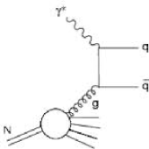
Figure 1: Boson-gluon-fusion (BGF) graph.

In perturbative quantum chromodynamics (PQCD) calculations the production of heavy quarks at HERA proceeds dominantly via the direct boson- gluon fusion (BGF)(Fig.1), where the photon interacts indirectly with a gluon in the proton by the exchange of a heavy quark pair [1-10]. In the BGF dynamic, the charm(bottom) quark is treated as a heavy quark and its contribution is realized by fixed- order perturbative theory. As to the measurements of HERA [11-15], the charm (bottom) contribution to the structure function at small $x$ is a large fraction of the total, since this value is approximately $30\%$ ($1\%$) fraction of the total. This behavior directly is related to the growth of the gluon distribution at small $x$. We know that the gluons couple only through the strong interaction, consequently the gluons are not directly probed in DIS. The only way to indirect contribution is via the $g{\rightarrow}q_{H}\bar{q}_{H}~{}(q_{H}=c,b)$ transition. This involves the computation of the BGF process $\gamma^{\star}g{\rightarrow}q_{H}\bar{q}_{H}$. This process can be created when the squared invariant mass of the hadronic final state has the condition that runs as follows $W^{2}{\geq}4m_{q_{H}}^{2}$.
In the framework of DGLAP (Dokshitzer- Gribov-Lipatov-Altarelli-Parisi) [16-18] dynamics, considering the heavy-flavour physics is in the framework of variable-flavor-number scheme (VFNS) [19,20]. In this scheme, the mass logarithms are resummed through all orders into a heavy quark density according to the DGLAP evolution equations. All logarithmic terms of the heavy flavor Wilson coefficients are obtained by factorization of this quantity into the massive operator matrix elements. The study of heavy flavor production can be done in deep inelastic electron-proton scattering, which was investigated experimentally at HERA and recently at LHC. These data for heavy quark production, have been proposed in the framework of the fixed-flavor-number scheme (FFNS)(where only light degrees of freedom are considered as active), that it was calculated for $F_{2}^{c}$ and $F_{2}^{b}$ [11-15].
The heavy flavor structure functions $F_{k}^{i}(x,Q^{2})$($k=2,L$ and $i=c,b$ ) are dependent to the parton distribution functions. In the small-$x$ range, further simplification is obtained by neglecting the contributions caused by incoming light quarks and antiquarks. This is justified because they vanish at LO and are numerically suppressed at NLO for small values of $x$, while the gluon contribution is a matter at this region [6-7]. In axial gauges, the leading double logarithms (i.e. $\ln(Q^{2})\ln(1/x)$) are generated by ladder diagrams in which the emitted gluons have strongly been ordered with respect to the transverse and longitudinal momenta. The sum of theses momenta predicts that the gluon distribution increases as $x$ decreases. Clearly this increase cannot go on indefinitely. When the density of gluons becomes too large, they can no longer be treated as free partons [21-22]. At very small $x$ we expect annihilation or recombination of gluons to occur and these shadowing corrections give rise to nonlinear terms in the evolution equation for the gluon distribution function. This picture allows us to write the GLR-MQ (Gribov, Levin, Ryskin, Mueller and Qiu) equation for the gluon distribution function at small-$x$ [23-24]. We expect the gluon correlations at small-$x$ to tame the behavior of the gluon distribution function. Therefore we observe that the heavy flavor structure functions (HFSFs) and also heavy reduced cross sections behaviors are tamed the saturation effects.
An important point in gluon saturation approach is the $x$-dependent saturation scale $Q_{s}^{2}(x)$, where it is the critical line between non-linear and linear effects and it is an intrinsic characteristic of a dense gluon system [25-26].
In this paper, we also investigate this non-linear behavior for the charm and bottom quarks at small-$x$ related to the GLR-MQ evolution equation. Then we will apply the geometric scaling parameterization in according with the critical line $Q^{2}=Q_{s}^{2}(x)$. We will do this, because the geometric scaling of the dipole cross section gives the similar scaling of the quantity $\alpha_{s}(Q^{2})\frac{xg(x,Q^{2})}{Q^{2}}$ that is dominant in the charm and bottom structure functions.
The content of our paper is as follows. In the next section we give a summary about heavy quark structure functions and color dipole model with starting gluon distribution along the critical line. Then we will study the heavy quark structure functions for $Q^{2}{\geq}Q_{s}^{2}(x)$ in sections 3-5, respectively. In Sec.6 we present the behavior of the HFSFs exponents at unshadowed and shadowed corrections to the gluon density behavior and also in geometrical scaling. Finally we give our conclusions in Sec.7.

2. A short theoretical input

In this section we briefly present the theoretical part of our analysis. The reader can be referred to the Refs.[27-36] for more details.
The heavy quark contributions $F_{k}^{i}(x,Q^{2},m^{2}_{i})$ to the proton structure function at small-$x$ (where only the gluon contributions are considerable) are given by this form

$$F_{k}^{i}(x,Q^{2},m^{2}_{i}) = 2e_{i}^{2}\frac{\alpha_{s}(\mu^{2})}{2\pi}\int_{1-\frac{1}{a}}^{1-x}dzC_{g,k}^{i}(1-z,\zeta)$$ (1)

$${\times}G(\frac{x}{1-z},\mu^{2}),$$

where $a=1+4\zeta(\zeta{\equiv}\frac{m_{i}^{2}}{Q^{2}})$, $G=xg$ is the gluon distribution function and $\mu^{2}$ denotes the factorization scale. Here $C^{i}_{g,k}$ are the heavy coefficient functions in BGF at LO and NLO analysis and in the NLO analysis

$$\alpha_{s}(\mu^{2})=\frac{4{\pi}}{\beta_{0}ln(\mu^{2}/\Lambda^{2})}-\frac{4\pi\beta_{1}}{\beta_{0}^{3}}\frac{lnln(\mu^{2}/\Lambda^{2})}{ln(\mu^{2}/\Lambda^{2})}$$ (2)

with $\beta_{0}=11-\frac{2}{3}n_{f},\beta_{1}=102-\frac{38}{3}n_{f}$ ($n_{f}$ is the number of active flavors).
At small-$x$, perturbative QCD predicts an increase in the gluon distribution tamed by saturation effects. The physical picture of this process is provided in the rest frame of the proton. In the small $x$ limit, the virtual photon splits into a $q\overline{q}$ color dipole followed by the interaction of this dipole with the color fields in the proton. The dipole cross section has been defined by [37]

$$\sigma_{dipole}(x,\mathbf{r})=\sigma_{0}(1-e^{-\mathbf{r}^{2}Q_{s}^{2}(x)/4}),$$ (3)

in which $r$ is the transverse separation of the $q\overline{q}$ pair and $Q_{s}(x)$ parameterized as $Q_{s}^{2}(x)=Q_{0}^{2}(x_{0}/x)^{\lambda}~{}GeV^{2}$. The important property of the dipole cross section is its geometric scaling (GS), which is a well-known property of DIS for small-$x$ values [38-41]. Therefore the proton cross section is dependent upon the single variable $\tau=Q^{2}/Q_{s}^{2}(x)$, as

$$\sigma_{\gamma^{*}p}(x,Q^{2})=\sigma_{\gamma^{*}p}(\tau).$$ (4)

3. Linear behavior for the evolution of the HFSFs

The heavy flavor structure functions (HFSFs) are described as Mellin convolutions between the gluon distribution $G(x,\mu^{2})$ and the Wilson coefficients $C_{k,g}^{i}(x,\frac{Q^{2}}{\mu^{2}})$ as

$$F_{k}^{i}(x,Q^{2})=C_{k,g}^{i}(x,\frac{Q^{2}}{\mu^{2}}){\otimes}G(x,\mu^{2}),~{}~{}(k=2\&L,i=c\&b)$$ (5)

here the Mellin convolutions is given by

$$f_{1}(x){\otimes}f_{2}(x){\equiv}\int_{x}^{1}\frac{dy}{y}f_{1}(y)f_{2}(\frac{x}{y}).$$ (6)

The $Q^{2}$ evolution equation for the HFSFs (Eq.5) is expressed in terms of these structure functions, as we have it:

$$\frac{{\partial}F^{i}_{k}(x,Q^{2})}{{\partial}\ln Q^{2}} = \sum_{n=1}n\frac{{d}{\ln}\alpha_{s}}{{d}\ln Q^{2}}F^{i,(n)}_{k}(x,Q^{2})+P_{gg}{\otimes}F^{i}_{k}(x,Q^{2})$$ (7)

$$+\frac{d{\ln}C_{k,g}^{i}}{d{\ln}Q^{2}}{\otimes}F^{i}_{k}(x,Q^{2}),$$

in which the corresponding physical evolution kernel $P_{gg}$ can be derived from DGLAP evolution equation at small-$x$ as it follows:

$$\frac{{\partial}G(x,\mu^{2})}{{\partial}{\ln}Q^{2}}=P_{gg}(x,\alpha_{s}){\otimes}G(x,\mu^{2}).$$ (8)

This kernel is corresponding to the massless Wilson coefficients in leading order (LO) up to next-to-next-to leading order (NNLO) [42-44], and also the heavy contributions are in leading order and next-to-leading order by using massive Wilson coefficients in the asymptotic region $Q^{2}>>m^{2}$.
According to the Regge pole approach, the distribution functions can be controlled by Pomeron exchange at small $x$, since these behaviors are correspondent to the BFKL (Balitskii-Fadin-Kuraev-Lipatov) Pomeron[45-48] ideas as extended by adding a hard Pomeron which describes the small-$x$ HERA data up to $Q^{2}$ of a few hundred GeV² values. The small-x asymptotic behavior for the gluon and heavy flavors can be exploited to the evolution equations of the HFSFs. Therefore, linear evolution of the HFSFs at small-$x$ can be found as

$$F_{k}^{i}(x,Q^{2})|_{x{\rightarrow}0}=\sum_{n=1}F^{i,(n)}_{k}(x,Q_{0}^{2})I_{k}^{i,(n)},$$ (9)

where

$$I_{k}^{i,(n)} = \exp(\int_{Q_{0}^{2}}^{Q^{2}}{d}\ln Q^{2}(\sum_{n=1}n\frac{{d}{\ln}\alpha_{s}}{{d}\ln Q^{2}}+P_{gg}{\otimes}x^{\lambda}$$ (10)

$$+\frac{{d}{\ln}C_{k,g}^{i}}{{d}\ln Q^{2}}{\otimes}x^{\lambda})).$$

Now, we have a compact small-$x$ formula for the heavy flavor ratio $R^{i}=\frac{F_{L}^{i}}{F_{2}^{i}}$ which greatly simplifies the extraction of $F^{i}_{2}$ from measurements of reduced heavy cross sections $\sigma_{r}^{i}$:

$$\sigma_{r}^{i}(x,Q^{2})=F^{i}_{2}(x,Q^{2})[1-\frac{y^{2}}{1+(1-y)^{2}}R^{i}(x,Q^{2})].$$ (11)

Therefore, we found a small-$x$ formula for the ratio $R^{i}$ by the following form

$$R^{i}(x,Q^{2}) = \frac{F_{L}^{i}(x,Q^{2})}{F_{2}^{i}(x,Q^{2})}=\frac{F^{i}_{L}(x,Q_{0}^{2})}{F^{i}_{2}(x,Q_{0}^{2})}{\times}$$

$$\exp(\int_{Q_{0}^{2}}^{Q^{2}}{d}\ln Q^{2}(\frac{{d}[{\ln}C_{L,g}^{i}-{\ln}C_{2,g}^{i}]}{{d}\ln Q^{2}}{\otimes}x^{\lambda})).$$

4. Nonlinear behavior for the evolution of the HFSFs

As mentioned above the HFSFs linear evaluation equation is based on a hard-Pomeron behavior for the gluon and heavy structure functions [49-56]. The gluon density increases with decreasing $x$ and we must reach the region in which gluon-gluon interactions confine the growth implied by this behavior concerning the gluon distribution, $G\sim x^{-\lambda}$, as this behavior will violate unitarity when $x{\rightarrow}0$. Thus, we discuss absorption effects which tame the violation of unitarity. At sufficient small-$x$ values two gluons in different cascades may interact and the gluon ladders fusion are generally important. Therefore the gluon density is decreasing and shadowing contributions can no longer be neglected [21-22,57-60]. Shadowing corrections, which take into account the fusion of $t$-channel gluons, modify the linear DGLAP equation for the gluon distribution by adding a negative term proportional to quadratic in $g(x,Q^{2})$. This picture allows us to write the GLR-MQ equation for the gluon distribution function behavior at small-$x$ symbolically as:

$$\frac{{\partial}xg(x,Q^{2})}{{\partial}{\ln}Q^{2}} = \frac{{\partial}xg(x,Q^{2})}{{\partial}{\ln}Q^{2}}|_{DGLAP}$$ (13)

$$-\frac{81\alpha^{2}_{s}\gamma}{16R^{2}Q^{2}}\int\frac{dy}{y}[yg(y,Q^{2})]^{2}.$$

The nonlinear shadowing term, ${\propto}-[g]^{2}$, arises from perturbative QCD diagrams which couple four gluons into two gluons so that two gluon ladders recombine into a single one. The minus sign occurs because the scattering amplitude corresponding to a gluon ladder is predominantly imaginary . Thus the equation (13) becomes nonlinear in $xg$. We neglect the quark-gluon emission diagrams due to their little importance on the rich gluon in small-$x$ region and we work under an approximation of neglecting contribution from the high twist gluon distribution $G_{HT}(x,Q^{2})$ [24].
In what follows it is convenient to use directly the reduced gluon distribution function behavior according to the Eq.13 as the $Q^{2}$ evolution of the HFSFs modified by

$$\frac{{\partial}F^{i}_{k}(x,Q^{2})}{{\partial}\ln Q^{2}} = \frac{{\partial}F^{i}_{k}(x,Q^{2})}{{\partial}\ln Q^{2}}[Eq.7]$$ (14)

$$-2e_{i}^{2}\frac{\alpha_{s}}{2\pi}\frac{\alpha^{2}_{s}\gamma}{R^{2}Q^{2}}\int_{1-\frac{1}{a}}^{1-x}dzC_{g,k}^{i}(1-z,\zeta)$$

$${\times}\frac{G^{2}(\frac{x}{1-z},\mu^{2})}{2\lambda}[1-(\frac{\chi}{1-z})^{2\lambda}].$$

Here $\chi=\frac{x}{x_{0}}$, where $x_{0}(=0.01)$ is the boundary condition that the gluon distribution joints smoothly the unshadowed region and $R$ is the radius of the proton. The first term is the linear evolution (Eq.7) and the second term is due to the 2-gluon density. Therefore the shadowing corrections to the HFSFs can be defined by Eq.14. To obtain a differential equation for shadowing corrections to the HFSFs, we write out the sum and the coefficient function explicitly. Consequently we find an inhomogeneous first-order differential equation which determines HFSFs shadowing corrections in terms of shadowed gluons. Eq. (14) can be rewritten in the following form:

$$\frac{{\partial}F^{i}_{k}(x,Q^{2})}{{\partial}\ln Q^{2}}-\eta(x,Q^{2})F^{i}_{k}(x,Q^{2})=-S^{i}_{k}(x,Q^{2}),$$ (15)

where

$$S^{i}_{k}(x,Q^{2})=2e_{i}^{2}\frac{\alpha_{s}}{2\pi}\frac{\alpha^{2}_{s}\gamma}{R^{2}Q^{2}}\int_{1-\frac{1}{a}}^{1-x}dzC_{g,k}^{i}(1-z,\zeta)$$

$${\times}\frac{G^{2}(\frac{x}{1-z},\mu^{2})}{2\lambda}[1-(\frac{\chi}{1-z})^{2\lambda}],$$ (16)

and

$$\eta(x,Q^{2})=(\sum_{n=1}n\frac{{d}{\ln}\alpha_{s}}{{d}\ln Q^{2}}+P_{gg}{\otimes}x^{\lambda}+\frac{d{\ln}C_{k,g}^{i}}{d{\ln}Q^{2}}{\otimes}x^{\lambda}).$$

The general solution of Eq. (15) where tames the behavior of the HFSFs at small-$x$ has the following form:

$$F^{i}_{k}(x,Q^{2}) = e^{\int_{Q_{0}^{2}}^{Q^{2}}\eta(x,Q^{2})d\ln Q^{2}}{\times}[F^{i}_{k}(x,Q_{0}^{2})$$

$$-\int_{Q_{0}^{2}}^{Q^{2}}S^{i}_{k}(x,Q^{2})e^{\int-\eta(x,Q^{2})d\ln Q^{2}}d\ln Q^{2}].$$

Therefore, shadowing corrections to the HFSFs modify the heavy reduced cross section and also the ratio of the HFSFs, as we will have:

$$\sigma_{r}^{i}(x,Q^{2}) = F^{i}_{2}(x,Q^{2})[Eq.18][1-\frac{y^{2}}{1+(1-y)^{2}}$$ (19)

$${\times}R^{i}(x,Q^{2})[Eq.20]],$$

where

$$R^{i}(x,Q^{2}) = \frac{F^{i}_{L}(x,Q^{2})}{F^{i}_{2}(x,Q^{2})}=[\frac{F^{i}_{L}(x,Q_{0}^{2})-\int_{Q_{0}^{2}}^{Q^{2}}S^{i}_{L}(x,Q^{2})e^{\int-\eta_{L}(x,Q^{2})d\ln Q^{2}}d\ln Q^{2}}{F^{i}_{2}(x,Q_{0}^{2})-\int_{Q_{0}^{2}}^{Q^{2}}S^{i}_{2}(x,Q^{2})e^{\int-\eta_{2}(x,Q^{2})d\ln Q^{2}}d\ln Q^{2}}]$$ (20)

$${\times}\exp(\int_{Q_{0}^{2}}^{Q^{2}}{d}\ln Q^{2}(\frac{{d}[{\ln}C_{L,g}^{i}-{\ln}C_{2,g}^{i}]}{{d}\ln Q^{2}}{\otimes}x^{\lambda})).$$

Equations 18-20 satisfy the requirements expected for shadowed distributions of the heavy quarks. These equations reduced to the unshadowed distributions (Eqs.9-12) when shadowing is negligible; that is, when $S^{i}_{k}(x,Q^{2}){\rightarrow}0$ which implies $G_{sat}{\rightarrow}\infty$. Finally the DGLAP+GLRMQ evolution joins smoothly into the DGLAP evolution when $x{\rightarrow}x_{0}$.

5. Geometrical scaling of the HFSFs

In the saturation model [61], the dipole cross section is bounded by an energy independent value $\sigma_{0}$ (Eq.3) which imposes the unitarity condition, $\sigma_{q\overline{q}}{\leq}\sigma_{0}$ with respect to the free parameters in the model[38-41]. These free parameters can be extracted from data within some specific models of DIS. In the Golec-Biernat-W$\ddot{u}$sthoff (GBW) model we see, $\sigma_{0}=23~{}mb$, $\lambda\cong 0.3$, $Q_{0}=1~{}GeV/c$ and $x_{0}=3{\times}10^{-4}$. The dipole cross section for a small $q\overline{q}$ dipole is related to the gluon density at scale $\mu^{2}$ as:

$$\sigma_{q\overline{q}}=\frac{\pi^{2}}{3}r^{2}\alpha_{s}xg(x,\mu^{2}).$$ (21)

For small $r{\ll}2R_{0}(x)$ in the saturation model (where $R_{0}(x)$ is the saturation scale at small-$x$), the gluon density found [38-41] by the following form:

$$xg(x,\mu^{2})=\frac{3}{4\pi^{2}\alpha_{s}}\frac{\sigma_{0}}{R_{0}^{2}(x)},$$ (22)

where at the geometric scale for the boundary $Q^{2}=Q^{2}_{s}(x)$ we have:

$$\frac{\alpha_{s}}{2\pi}xg(x,Q^{2}=Q^{2}_{s}(x))=r_{0}x^{-\lambda},$$ (23)

with $r_{0}=\frac{3}{8{\pi^{3}}}{\sigma_{0}}{x_{0}^{\lambda}}$. Also R.S.Thorne [62] used the relationship between the dipole cross section and the unintegrated gluon distribution and showed that the gluon distribution at fixed coupling has this behavior:

$$xg(x,Q^{2}) = \frac{3\sigma_{0}}{4{\pi^{2}}\alpha_{s}}(-Q^{2}e^{{-Q^{2}}(x/x_{0})^{\lambda}}+(x_{0}/x)^{\lambda}$$ (24)

$${\times}(1-e^{{-Q^{2}}(x/x_{0})^{\lambda}})).$$

In order to be able to study the formal heavy flavor production limit, the Bjorken variable $x=x_{B}$ was modified into the one as follows:

$$x=x_{B}(1+\frac{4m^{2}_{hf}}{Q^{2}}),$$ (25)

when a pair of heavy quarks $H\overline{H}$ ($c\overline{c}$ or $b\overline{b}$) are produced in the final state. Therefore the gluon distribution can be evaluated for heavy quarks according to Eq.24. This is consistent with a general-mass-variable flavor number schemes (GM-VFNS) [63]. In this case, the parameters obtained from the best fit were $\sigma_{0}=29.12~{}mb$, $\lambda=0.277$ and $x_{0}=0.41{\times}10^{-4}$ [38-41]. Because the data for the bottom component $\sigma^{b}{\sim}\frac{F_{2}^{b}}{Q^{2}}$ are not suitable for scaling analysis( since they contain two few points [11-15]), therefore we used the charm parameters in our determination for bottom structure functions.
Therefore the dipole picture at the geometric scaling is suitable for HFSFs analysis . If the characteristic size of the $q_{H}\overline{q}_{H}$-pair is much smaller than the saturation radius, with decreasing $x$, it can show that the behavior of the HFSFs at the scale $<\mu^{2}>$ is given by

$$F_{k}^{i}(x,Q^{2})=r_{0}Q_{s}^{2}(x)[C_{k,g}^{i}(x,\frac{Q^{2}}{\mu^{2}}){\otimes}x^{\lambda}].$$ (26)

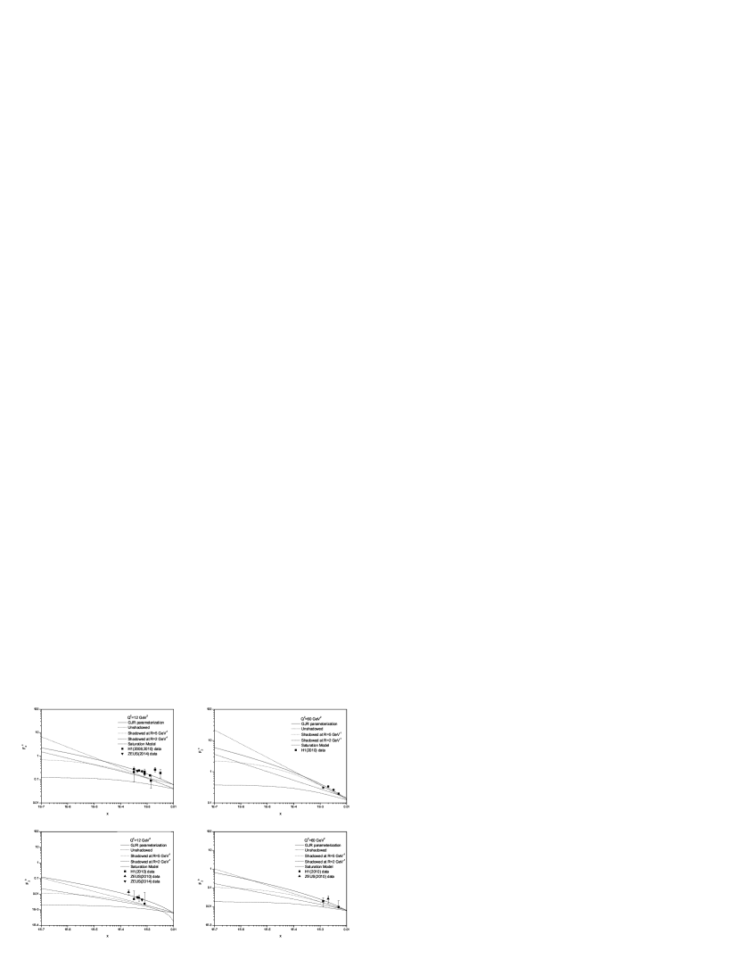
Figure 2: Heavy flavor structure functions $F_{2}^{i}(x,Q^{2})$ as a function of the Bjorken variable $x$ at $Q^{2}$ values $12$ and $60~{}GeV^{2}$ in comparison with the experimental data from ZEUS and H1 Collaborations [11-15] accompanied by total errors and GJR parameterization [64]. The unshadowed and shadowed corrections and also the saturation model concerning the geometrical scaling are shown in this figure.

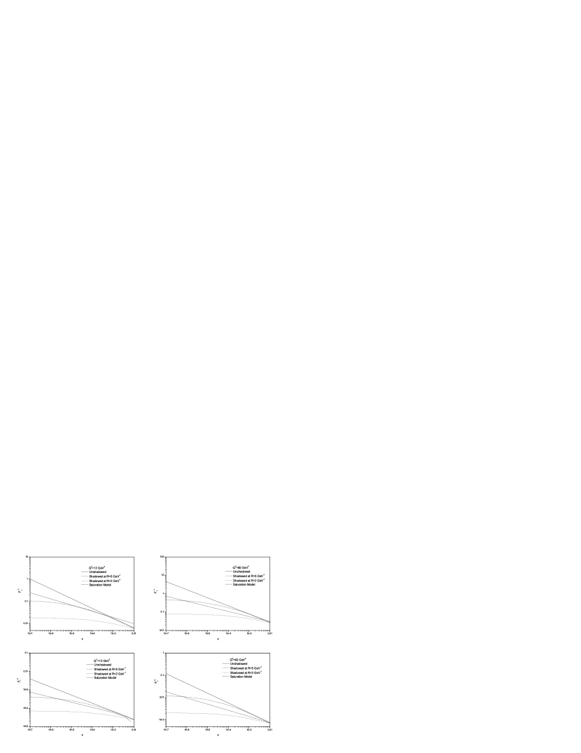
Figure 3: Heavy flavor longitudinal structure functions $F_{L}^{i}(x,Q^{2})$ as a function of the Bjorken variable $x$ at $Q^{2}$ values $12$ and $60~{}GeV^{2}$. The unshadowed and shadowed corrections and also the saturation model concerning the geometrical scaling are shown in this figure.

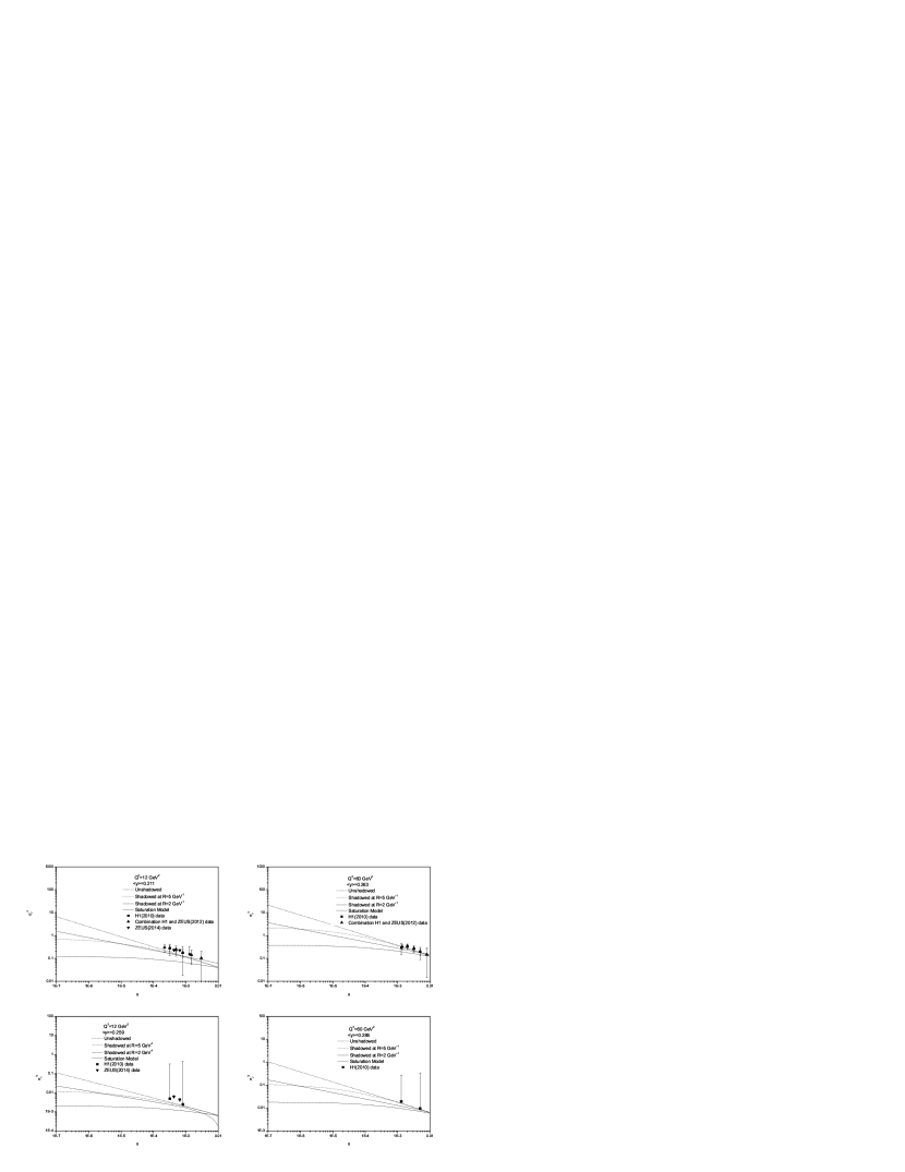
Figure 4: Heavy flavor reduced cross section $\sigma_{r}^{i}(x,Q^{2})$ as a function of the Bjorken variable $x$ at $Q^{2}$ values $12$ and $60~{}GeV^{2}$ in comparison with the experimental data from ZEUS and H1 Collaborations [11-15] accompanied by total errors at inelasticity $<y>$. The unshadowed and shadowed corrections and also the saturation model concerning the geometrical scaling are shown in this figure.

We summarized our results in sections 3-5 at Figs.2-4. In these figures the results of calculation for charm and bottom structure functions, longitudinal structure functions and reduced cross sections are shown at $Q^{2}=12$ and $60~{}GeV^{2}$ respectively. We determined the HFSFs and reduced cross sections in linear behavior (unshadowed) when shadowing is neglected. It was also made clear in nonlinear behavior (shadowed) at $R=5~{}GeV^{-1}$ where the gluons are spread throughout the entire proton and at $R=2~{}GeV^{-1}$ where the gluons are concentrated in hot-spots within the proton. We observe that these behaviors for the heavy quarks functions are tamed at small-$x$. The reduced cross sections are determined at the average inelasticity $<y>$ in according with the H1 data. We compared our results with GJR parameterization [64], the ZEUS and H1 data [11-15]. We can observe that there are a well agreement between our unshadowed, shadowed and saturation results with the experimental data accompanied by total errors.

6. Heavy flavor exponents behavior

In the double asymptotic limit, the behavior of the gluon distribution is expected to rise approximately as a power of $x$ towards small-$x$. Because, the behavior of the HFSFs and heavy flavor reduced cross sections are dependent on the gluon distribution behavior directly. Therefore we consider the power-like behavior of the HFSFs at small-$x$ as $f_{\xi}^{i}{\propto}x^{-\lambda_{\xi}^{i}(x,Q^{2})}$ where $f_{\xi}=F_{2},F_{L}$ and $\sigma_{r}$. The logarithmic $x$-derivative of the heavy flavor functions concerning $\ln(\frac{1}{x})$ can be defined [65] as:

$$H_{\xi}^{i}(x,Q^{2})=\frac{\partial{\ln}f_{\xi}^{i}(x,Q^{2})}{\partial{\ln}(1/x)}.$$ (27)

Here we would like to consider the relation between the effective intercept $\lambda_{\xi}^{i}$ for heavy flavor functions and logarithmic-$x$ derivatives of the heavy flavor functions where

$$H_{\xi}^{i}(x,Q^{2})=\lambda_{\xi}^{i}(x,Q^{2})+{\ln}\frac{1}{x}\frac{\partial\lambda_{\xi}^{i}(x,Q^{2})}{\partial{\ln}(1/x)}.$$ (28)

For unshadowed heavy flavor functions (Figs.2-4) we used the Pomeron intercept in our determinations, therefore the effective intercept and $x$-slop strictly coincide with the hard Pomeron intercept as we considered this behavior for the gluon distribution at small-$x$. Therefore in this case, we will come into the below:

$$H_{\xi}^{i}(Q^{2})=\lambda_{\xi}^{i}(Q^{2})=0.44.~{}~{}~{}(i=c,b)$$ (29)

When we consider the saturation effects [25-26] on the charm functions, the charm exponents obtained will be follows:

$$H_{\xi}^{c}(Q^{2})=\lambda_{\xi}^{c}(Q^{2})=0.277.$$ (30)

But this value is not coincident with the bottom functions, since we do not have enough data for bottom component in scaling analysis. One can see that exponents obtained for heavy flavor functions at the shadowed region are dependent on the saturation scale and $R$ parameter. For the nonlinear evaluation equation we can observe that:

$$H_{\xi}^{i}(x,Q^{2}){\neq}\lambda_{\xi}^{i}(x,Q^{2}).$$ (31)

For heavy functions at $R=5$ and $2~{}GeV^{-1}$, there is not a linear function when we fit it to all data because inequality (31) is correct. For $R=5~{}GeV^{-1}$ there is a second-order function and for $R=2~{}GeV^{-1}$ there is a three-order function. So we conclude that at nonlinear evolution equations, the heavy exponents are dependent on $x$ and $R$ values, for the shadowed heavy flavors are dependent on the values $x$, $Q^{2}$ and $R$, i.e., ($\lambda_{\xi}^{i,shadowed}=\lambda(x,Q^{2},R)$).
In addition to the $x$-slope, we want to consider the logarithmic derivative of the heavy functions with respect to $\ln Q^{2}$, as the $Q^{2}$-slopes are defined by:

$$\frac{\partial f_{\xi}^{i}(x,Q^{2})}{\partial{\ln}(Q^{2})}.$$ (32)

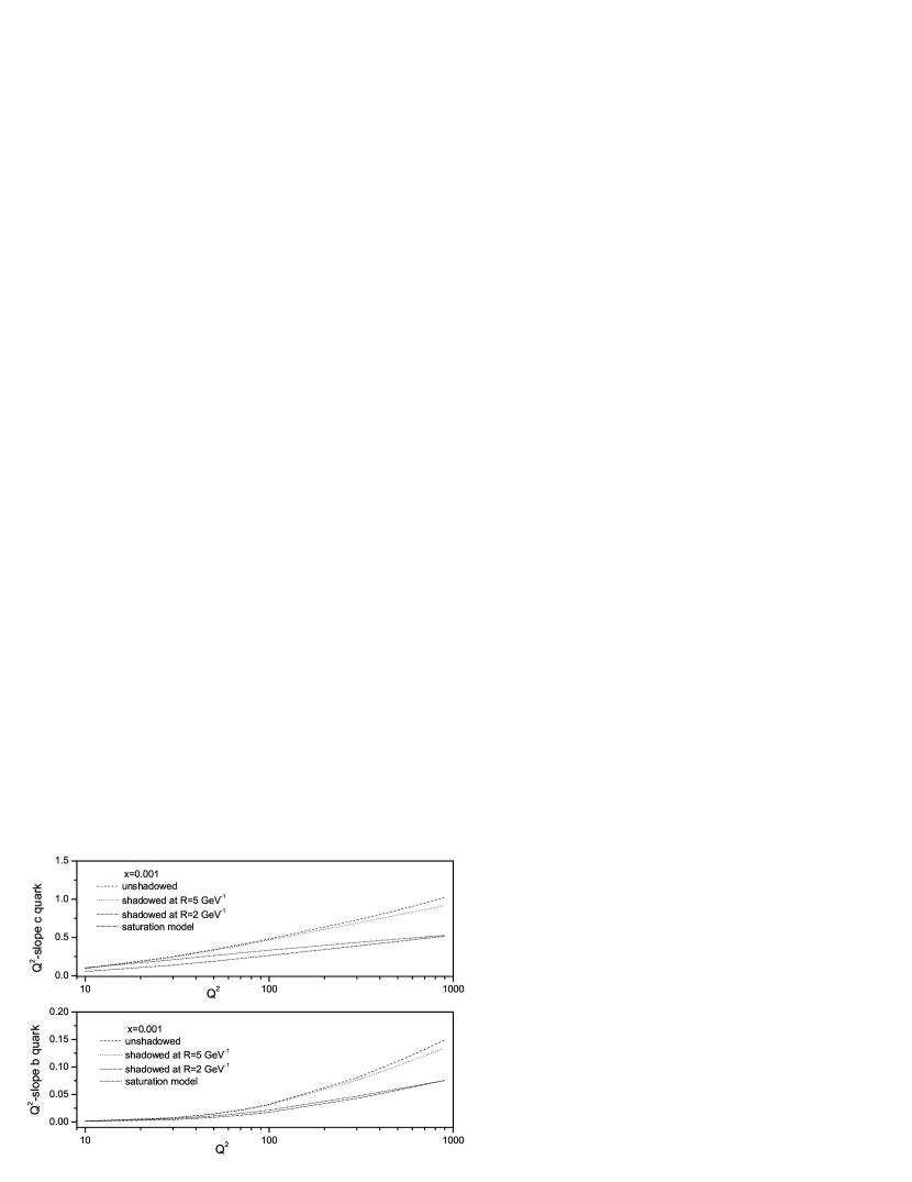
Figure 5: $Q^{2}$-slope heavy flavor structure functions ($\partial{F_{2}^{i}}/\partial{\ln{Q^{2}}}$) as function of $Q^{2}$ at $x=0.001$. Our results shown for unshadowed and shadowed corrections and also for saturation model with respect to the geometrical scaling in $Q^{2}$-slope heavy flavor structure functions.

Figure 5 shows the derivative as a function of $Q^{2}$ for $x=0.001$ value. The derivative is observed to have a logarithmically approximate rise with $Q^{2}$ for $F_{2}^{i}(x,Q^{2})$. The ${\ln}(Q^{2})$ dependence of $F_{2}^{i}(x,Q^{2})$ is observed to be non-linear. It can be well described by a quadratic expression, since for each of heavy quarks these derivatives can be described by the function $b(x)+2c(x)\ln(Q^{2})$. The shape of these derivatives reflect the behavior of the gluon distribution in the associated kinematic range.
This scaling violation shows the transition from soft to hard dynamics. We give this scaling violation to the function $\eta(Q^{2})$ then we consider the heavy functions behavior as a fixed power of $x$:

$$f_{\xi}^{i}(x,Q^{2})=\eta_{\xi}^{i}(Q^{2})x^{-\lambda}.$$ (33)

It would be implied that the Mellin transform $f_{\xi}^{i}(j,Q^{2})$ would have a pole at $j=1+\lambda$, where this singularity referred to as the hard-Pomeron singularity [49-56]. We conclude that the power $\lambda^{,}$s in Eqs.29 and 30 are not dependent on $Q^{2}$ and theses powers have got fixed values. In our determinations (Fig.5), each of theses coefficient functions $\eta_{\xi}^{i}(Q^{2})$ vanished in a way that $Q^{2}{\rightarrow}0$. In Fig.6 we compared our results for $\eta_{2}^{c}(Q^{2})$ and $\eta_{2}^{b}(Q^{2})$ with DL model [49-56] and color dipole model (CDM) [1-4]. These results are comparable with others.

7. Conclusions

We have studied several aspects of the heavy flavors functions behavior at small-$x$. To do this, we assumed that the heavy parton density obeys power-laws having effective power. Therefore we have applied the hard Pomeron and saturation methods in obtaining the heavy flavors functions considering H1 and ZEUS data. We have shown that geometrical scaling in DIS works well up to the heavy flavors functions with a constant exponent. The merit of this exponent is mainly due to its relation with the gluon density at small-$x$. Results obtained suggest that geometrical scaling in heavy production is basically the same as for the inclusive DIS. The value of shadowed exponents are different from the one obtained for unshadowed corrections and geometrical scaling in heavy functions. This difference is due to the shadowing corrections on the heavy functions. Indeed the value of the shadowed correction on the exponents depends on how exactly the gluon ladders couple to the proton or on how the gluons are distributed within the proton, especially in hot-spot point. As a result, the coefficient functions ($\eta(Q^{2})$) are dependent on the $Q^{2}$ scale and the effective powers are constant. We obtained our results for the $\eta(Q^{2})$ and compared them with DL and CD models.

Acknowledgment

The authors would like thank Y.Refahiyat for his careful revising of the paper with regard to its language.

References
1. N.N.Nikolaev and V.R.Zoller, Phys.Atom.Nucl73, 672(2010).
2. N.N.Nikolaev and V.R.Zoller, Phys.Lett.B 509, 283(2001).
3. N.N.Nikolaev, J.Speth and V.R.Zoller, Phys.Lett.B473, 157(2000).
4. R.Fiore, N.N.Nikolaev and V.R.Zoller, JETP Lett90, 319(2009).
5.A. V. Kotikov, A. V. Lipatov, G. Parente and N. P. Zotov Eur. Phys. J.  C 26, 51 (2002).
6. A. Y. Illarionov, B. A. Kniehl and A. V. Kotikov, Phys. Lett. B 663, 66 (2008).
7. A. Y. Illarionov and A. V. Kotikov, Phys.Atom.Nucl. 75, 1234 (2012).
8. N.Ya.Ivanov, and B.A.Kniehl, Eur.Phys.J.C59, 647(2009).
9. N.Ya.Ivanov, Nucl.Phys.B814, 142(2009).
10. J.Blumlein, et.al., Nucl.Phys.B755, 272(2006).
11. F.D. Aaron et al. [H1 Collaboration],Phys.Lett.b665, 139(2008).
12. F.D. Aaron et al. [H1 Collaboration],Eur.Phys.J.C65,89(2010).
13. H.Abramovicz et. al., [ZEUS Collaboration], arXiv:hep-ex/1005.3396(2010).
14. H.Abramovicz et. al., [ZEUS Collaboration], arXiv:hep-ex/1405.6915(2014).
15. H.Abramovicz et. al., [Combination H1 and ZEUS Collaboration], arXiv:hep-ex/1211.1182(2012).
16.Yu.L.Dokshitzer, Sov.Phys.JETP 46, 641(1977).
17. G.Altarelli and G.Parisi, Nucl.Phys.B 126, 298(1977).
18. V.N.Gribov and L.N.Lipatov, Sov.J.Nucl.Phys. 15, 438(1972).
19. M.A.G.Aivazis, et.al., Phys.Rev.D50, 3102(1994).
20. J.C.Collins, Phys.Rev.D58, 094002(1998).
21. J.Kwiecinski, A.D.Martin and P.J.Sutton, Phys.Rev.D44, 2640(1991).
22. J.Kwiecinski, A.D.Martin, R.G.Roberts and W.J.Stirling, Phys.Rev.D42, 3645(1990).
23. L.V.Gribov, E.M.Levin and M.G.Ryskin, Phys.Rep.100, 1(1983).
24. A.H.Mueller and J.Qiu, Nucl.Phys.B268, 427(1986).
25. K. Golec-Biernat, Acta.Phys.Polon.B35, No.12, 3103(2004).
26. F. Carvalho, et.al., Phys.Rev.C79, 035211(2009).
27. M.Gluk, E.Reya and A.Vogt, Z.Phys.C67, 433(1995).
28. M.Gluk, E.Reya and A.Vogt, Eur.Phys.J.C5, 461(1998).
29. E.Laenen, S.Riemersma, J.Smith and W.L. van Neerven, Nucl.Phys.B 392, 162(1993).
30. S. Catani, M. Ciafaloni and F. Hautmann, Preprint CERN-Th.6398/92, in Proceeding of the Workshop on Physics at HERA (Hamburg, 1991), Vol. 2., p. 690.
31. S. Catani and F. Hautmann, Nucl. Phys. B 427, 475(1994).
32. S. Riemersma, J. Smith and W. L. van Neerven, Phys. Lett. B 347, 143(1995).
33. J.Kwiecinski and A.M.Stasto, Phys.Rev.D66, 014013(2002).
34. A.M.Stasto, et.al., Phys.Rev.Lett86, 596(2001).
35. E.Iancu, et.al., Phys. Lett. B590, 199(2004).
36. H.Kowalski and D.Teaney, Phys. Rev.D68, 114005(2003).
37. K. Golec-Biernat and M.Wusthoff, Phys.Rev.D59, 014017(1998).
38. K. Golec-Biernat, J.Phys.G28, 1057(2002).
39. K. Golec-Biernat,Acta.Phys.Polon.B33, 2771(2002).
40. J.Bartles, et.al., Phys.Rev.D66, 014001(2002).
41. J.Bartles, et.al.,Acta.Phys.Polon.B33, 2853(2002).
42. S.Moch and J.A.M.Vermaseren, Nucl.Phys.B573, 853(2000).
43. S.Moch, J.A.M.Vermaseren and A.Vogt, Phys.Lett.B606, 123(2005).
44. J.A.M.Vermaseren, A.Vogt and S.Moch,, Nucl.Phys.B724, 3(2005).
45. E.A.Kuraev, L.N.Lipatov and V.S.Fadin, Phys.Lett.B 60, 50(1975).
46. E.A.Kuraev, L.N.Lipatov and V.S.Fadin, Sov.Phys.JETP 44, 433(1976).
47. E.A.Kuraev, L.N.Lipatov and V.S.Fadin, ibid. 45, 199(1977).
48. Ya.Ya.Balitskyii and L.N.Lipatov, Sov.J.Nucl.Phys. 28, 822(1978).
49. A.Donnachie and P.V.Landshoff, Z.Phys.C 61, 139(1994).
50. A.Donnachie and P.V.Landshoff, Phys.Lett.B 518, 63(2001).
51. A.Donnachie and P.V.Landshoff, Phys.Lett.B 533, 277(2002).
52. A.Donnachie and P.V.Landshoff, Phys.Lett.B 470, 243(1999).
53. A.Donnachie and P.V.Landshoff, Phys.Lett.B 550, 160(2002).
54. R.D.Ball and P.V.landshoff, J.Phys.G26, 672(2000).
55. J.R.Cudell, A.Donnachie and P.V.Landshoff, Phys.Lett.B 448, 281(1999).
56. P.V.landshoff, arXiv:hep-ph/0203084 (2002).
57. K.J.Eskola, et.al., Nucl.Phys.B660, 211(2003).
58. K.Kutak and A.M.Stasto, Eur.Phys.J.C41, 343(2005).
59. M.Kazlov and E.Levin, Nucl.Phys. A764, 498 (2006).
60. M.A.Kimber, J.Kwiecinski and A.D.Martin, Phys.Lett. B508, 58(2001).
61. K.Golec-Biernat, arXiv:hep-ph/0812.1523(2008).
62. R.S.Thorne, Phys.Rev.D71, 054024(2005).
63. G.Beuf, C.Royon and D.Salek, arXiv:hep-ph/0810.5082(2008).
64.M. Gluck, P. Jimenez-Delgado, E. Reya, Eur.Phys.J.C53,355(2008).
65. P.Desgrolard et.al., JHEP02, 029(2002).

Figure 6: The coefficients $\eta_{2}^{i}(Q^{2})$ from fits of the form $F^{i}_{2}(x,Q^{2})=\eta_{2}^{i}(Q^{2})x^{-\lambda}$ to the shadowed and unshadowed corrections compared to DL model [49-56] and color dipole model (CDM) [1-4].