Junctions of surface operators and
categorification of quantum groups

Abstract:

We show how networks of Wilson lines realize quantum groups ${\mathbf{U}}_{q}(\mathfrak{sl}_{m})$, for arbitrary $m$, in 3d $SU(N)$ Chern-Simons theory. Lifting this construction to foams of surface operators in 4d theory we find that rich structure of junctions is encoded in combinatorics of planar diagrams. For a particular choice of surface operators we make a connection to known mathematical constructions of categorical representations and categorified quantum groups.






CALT-TH 2015-040

1 Introduction

In this paper we develop a physical framework for categorification of quantum groups, which is consistent with (and extends) the physical realization of homological knot invariants as $Q$-cohomology of a certain brane system in M-theory (that we review in section 4).

Our starting point will be the celebrated relation between quantum groups and Chern-Simons TQFT in three dimensions. Even though it has a long history, many aspects of this relation remain mysterious, even with respect to some of the most basic questions. For instance, quantum groups are usually defined via generators and relations, which are not easy to “see” directly in Chern-Simons gauge theory. Instead, one can see certain combinations of the generators that implement braiding of Wilson lines [1].

The realization of quantum groups we discuss in this paper is also based on Chern-Simons gauge theory, but in constrast to the conventional one, it allows for gauge group and quantum group to be of completely different rank! Moreover, the quantum group generators have an immediate and very concrete interpretation. This approach is based on networks of Wilson lines and gives a physical realization of the skew Howe duality, which was introduced in the context of knot homology in [2]: As we will show in section 2, upon concatenation, networks of Wilson lines exhibit quantum group relations, which for the Lie algebra $\mathfrak{g}=\mathfrak{sl}_{2}$ take a very simple form:

$$KK^{-1}=1=K^{-1}K\,,$$

$$KE=q^{2}EK\,,\qquad KF=q^{-2}FK$$ (1)

$$\left[E,F\right]={K-K^{-1}\over q-q^{-1}}\,.$$

Here, the quantum variable $q$ is related to the Chern-Simons coupling constant in the usual way, c.f. (10). What is not usual is that configurations of $m$ Wilson lines in totally antisymmetric representations

$$R_{1}\otimes\ldots\otimes R_{m}\;=\;\Lambda^{k_{1}}{\mathbb{C}}^{N}\otimes\ldots\otimes\Lambda^{k_{m}}{\mathbb{C}}^{N}$$ (2)

are interpreted as weight spaces of quantum $\mathfrak{sl}_{m}$, on which the Chevalley generators act by adding extra Wilson line segments. This idea is due to [3]. So, generators and relations of the quantum group have a very concrete realization (shown in Figures 14 and 10, respectively); and the rank $m-1$ of the quantum group has nothing to do with the rank $N-1$ of Chern-Simons gauge theory. Instead it is determined by the number of incoming (equally, outgoing) Wilson lines.

By categorifying representation theory, one usually means replacing weight spaces, such as (2), by graded categories $\mathfrak{R}_{\lambda}$ on which raising and lowering operators act as functors, c.f. [4, 5, 6, 7, 8]. The quantum group itself is promoted to a 2-category $\dot{\mathcal{U}}$, for which $\mathfrak{R}_{\lambda}$ is a 2-representation, as illustrated in Figure 1. Sounds a bit scary, doesn’t it?

Figure 1: Categorified representation theory and categorified skew Howe duality.

Luckily, the rich and abstract structure of categorical representations and categorified quantum groups can be made very “user-friendly” and intuitive in the diagrammatic approach recently developed by Khovanov and Lauda [9, 10, 11, 12] (see [13, 14, 15] for excellent expositions and [16] for a related algebraic construction). One of our main goals is to provide a physical realization of this diagrammatic approach.

In the context of quantum field theories, categorification can be achieved by adding a dimension, and networks of Wilson line operators used to realize quantum groups in Chern-Simons theory become foams of surface operators in 4d. Indeed, foams have been related to Khovanov-Lauda diagrams in the math literature in [17, 18]. The physical realizations of foams discussed here are built by sewing surface operators along 1d junctions, which are interesting in their own right and so far did not even appear in the physics literature. In section 3, we will not only present evidence that BPS junctions of surface operators exist, but we will also discuss various applications, ranging from math to physics.

In fact, the relevant surface operators [19, 20] have already been used to construct group actions on categories (notably, in the context of the geometric Langlands program [21]) and to realize many elements of geometric representation theory [22]. In these realizations, as well as in many other similar problems, groups acting on categories are generated by codimension-$1$ walls (interfaces) acting on categories of boundary conditions. The group law comes from the “fusion” product of interfaces. This is an instance of the well known fact that the algebraic structure of various operators and defects in $(n+1)$-dimensional topological quantum field theories is governed by $n$-categories (see e.g. [20] for a review).

Our physical realization of categorified quantum groups is conceptually similar, but with several twists. One way to describe it is to consider the world-volume theory on the foam of surface operators. By moving the $m$ parallel surface defects representing the $\mathfrak{sl}_{m}$ weight spaces close together we can describe the world-volume theory of the combined system as tensor product of the theories on the individual surface operators. Junctions of surface operators introduce interactions between tensor factors along $1$-dimensional loci, and are incorporated by interfaces between generally different 2d theories. For instance, collapsing the $x^{2}$-direction of the configuration of surface operators on the left of Figure 2, the combined world-volume theory can be described by a 2d theory in the $(x^{0},x^{1})$-plane. The surface operator supsended along the $x^{2}$-direction introduces a 1d interface.

Now, while in the spririt of the remark above the structure of a 2d TQFT is encoded in a $1$-category, different 2d TQFTs together with interfaces between them form a $2$-category, whose objects are not boundary conditions, but rather the different 2d theories. $1$-morphisms are interfaces, and $2$-morphisms are interface changing fields. As a bonus, these $2$-categories come with $2$-representations on the categories of boundary conditions of the 2d TQFTs.

It is in this way that we extract the building blocks of categorified quantum groups $\dot{\mathcal{U}}$ out of foams of surface operators: $\mathfrak{sl}_{m}$ weight spaces correspond to tensor products of the world-volume theories of $m$ surface operators, and the generators of the quantum group are realized as interfaces between them.

In fact, this 2d perspective on surface operators and their junctions provides a physical realization of the planar diagrams of Khovanov-Lauda [9, 10, 11, 12] and vast generalizations, for more general types of surface operators.

There are various ways to describe relevant 2d TQFTs, and in this paper we mainly consider two variants: one is based on topological Landau-Ginzburg (LG) models, while the second involves the UV topological twist of sigma-models whose targets are certain flag-like subspaces of affine Grassmannians which play an important role in the geometric Satake correspondence. We generally favor the former, where interfaces and their compositions are easier to analyze using matrix factorizations [23].

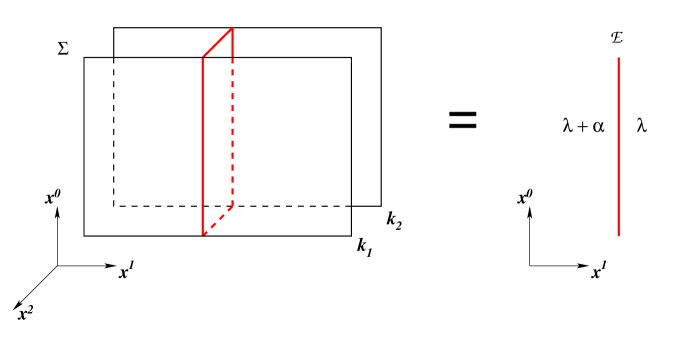
Figure 2: Projecting $\Sigma$ onto $(x^{0},x^{1})$ plane gives a product of Landau-Ginzburg theories, in which junctions (singular edges of $\Sigma$) are represented as interfaces.

In the Landau-Ginzburg approach (described in detail in section 4) the 2d space-time is precisely the plane on which the planar diagrams (with dots on the lines) of Khovanov-Lauda are drawn. Each 2d region of the plane colored by the highest weigh $\lambda$ defines a LG model or, to be more accurate, a product of LG models. It is basically a projection of $\Sigma$ from the three-dimensional space — that later in the text we parameterize with $(x^{0},x^{1},x^{2})$ — to a two-dimensional plane $(x^{0},x^{1})$. Then, LG interfaces describe transitions between different sheets of $\Sigma$, regarded as a multi-cover of the $(x^{0},x^{1})$-plane, c.f. Figure 2. These 1-dimensional interfaces (defects) are precisely the arcs in the planar diagrams of [9, 10, 11, 12]:

$$\begin{array}[]{ccccc}\vspace{0.1cm}\text{region on a plane}&\quad\leftrightarrow&\text{weight space \eqref{RRRweight}}&\quad\leftrightarrow&\text{LG model }LG_{k_{1}}\otimes\ldots\otimes LG_{k_{m}}\\ \vspace{0.1cm}\text{lines}&\leftrightarrow&\text{1-morphisms}&\leftrightarrow&\text{interfaces between LG models}\\ \text{dots}&\leftrightarrow&\text{2-morphisms}&\leftrightarrow&\text{interface changing fields}\end{array}$$

The reader is invited to use this dictionary to translate virtually any question in one subject to a question in another. For example, it would be interesting to study 2-categories that one finds for more general types of surface operators in various gauge theories, and interfaces in Landau-Ginzburg models, other than examples studied in this paper. Mathematically, they should lead to interesting generalizations of the Khovanov-Lauda-Rouquier (KLR) algebras [10, 11, 16]. Conversely, it would be interesting to identify surface operators and LG interfaces for mathematical constructions generalizing $\dot{\mathcal{U}}$.

In summary, if you are studying junctions of surface operators or interfaces in Landau-Ginzburg models, most likely you are secretly using the same mathematical structure — and, possibly, even the same diagrams — as those categorifying representations and quantum groups, or interesting generalizations thereof.

2 Junctions of Wilson lines and quantum groups

In this section, we will discuss Wilson lines in $SU(N)$ Chern-Simons theory and their junctions. We will show that (upon concatenation) certain networks of Wilson lines satisfy the defining relations of (Lusztig’s idempotent form [24] of) the quantum groups $\dot{\mathbf{U}}_{q}(\mathfrak{sl}_{m})$.

We start by reviewing the necessary techniques from [25, 26, 27] in section 2.1. In section 2.2, we explore various relations satisfied by networks of Wilson lines and their junctions, which surprisingly include the quantum group relations. We give an explicit derivation of one such relation, relegating the rest to Appendix A. Then, by playing with $m$ strands, in section 2.3 we (re)discover the representation category of the quantum group of $\mathfrak{sl}_{m}$. This gives a physical realization of the diagrammatic approach of Cautis-Kamnitzer-Morrison [3] to quantum skew Howe duality. Finally, in section 2.4, we give an a priori explanation why categorification of these beautiful facts should involve surface operators and their junctions, leading us into sections 3 and 4.

2.1 Junctions of line operators

Our starting point is Chern-Simons theory in three dimensions with gauge group $G=SU(N)$. The action on a closed $3$-manifold $M_{3}$ is given by

$$S_{CS}=\frac{\kappa}{4\pi}\int_{M_{3}}(A\wedge dA+\frac{2}{3}A\wedge A\wedge A).$$ (3)

where $A$ is an $SU(N)$-gauge connection on $M_{3}$, and the coupling constant $\kappa\in{\mathbb{N}}$ is usually called the “level.”

The most important (topological) observables of this theory are derived from the parallel transport with respect to $A$: To a path $\Gamma\subset M_{3}$ and a representation $R$ of the gauge group one associates the Wilson line

$$U_{R}(\Gamma)={\mathcal{P}}\exp\left(\int_{\Gamma}\rho_{R}(A)\right):~{}~{}~{}R\longrightarrow R\,.$$ (4)

Here ${\mathcal{P}}$ denotes path-ordering, and $\rho_{R}$ is the associated representation on the Lie algebra. For an open path $\Gamma$ such $U_{R}(\Gamma)$ is not gauge invariant, but one can form gauge invariant combinations, such as the familiar Wilson loops

$$W_{R}(\Gamma)={\rm tr}_{R}\,U_{R}(\Gamma)$$ (5)

by closing the path $\Gamma$. More general gauge invariant combinations can be associated to networks of Wilson lines [26] by forming junctions of Wilson lines in representations $R_{1},\ldots,R_{n}$ and contracting the corresponding observables $U_{R_{i}}$ with invariant tensors

$$\epsilon\;\in\;\text{Hom}(R_{1}\otimes\ldots\otimes R_{n},{\mathbb{C}})\,.$$ (6)

The latter correspond to additional junction fields, which need to be specified along with representations of Wilson lines in order define the observable.

Figure 3: (a) A trivalent network of Wilson lines and the corresponding gauge invariant observable. (b) Trivalent junctions of Wilson lines in antisymmetric representations: Labels $k$ refer to representations $\Lambda^{k}\square$.

For instance, to the graph in Figure 3(a), one can associate an observable by contracting the Wilson lines $U_{a}(\Gamma_{a})$, $U_{b}(\Gamma_{b})$ and $U_{c}(\Gamma_{c})$ with invariant tensors $\epsilon\in\overline{a}\otimes\overline{b}\otimes\overline{c}$ in the “incoming” junction and $\widetilde{\epsilon}\in a\otimes b\otimes c$ in the “outgoing” junction of the graph. Here $\overline{R}$ denotes the dual representation. (The Wilson lines carry gauge indices $i,j$ of representation $a$, $i^{\prime},j^{\prime}$ of $b$, and $i^{\prime\prime},j^{\prime\prime}$ of $c$, respectively. After contracting the gauge indices of Wilson lines via $\epsilon$ and $\widetilde{\epsilon}$, we obtain a gauge invariant observable.)

In the following we will mostly consider Wilson lines in totally antisymmetric representations $\wedge^{k}\square$, of the fundamental representation $\square$ of $SU(N)$, which for ease of notation we will just label by $k$. These Wilson lines admit two possible trivalent junctions, depicted in Figure 3(b), which are dual to each other. Since $Hom(\Lambda^{k_{1}}\square\otimes\Lambda^{k_{2}}\square,\Lambda^{k_{1}+k_{2}}\square)$ is one-dimensional, there is just one possible junction field, whose normalization we will fix shortly. We can then omit the labels of the junctions. As it turns out, junctions of more than three such Wilson lines can all be factorized into trivalent junctions, c.f. Figure 10(a).

In order to unambiguously define Wilson line invariants in the quantum theory, a framing, i.e. the choice of orthogonal vector fields along the Wilson lines is required, which fit together in the junctions. This is in particular needed to regularize the self-linking number of Wilson loops. In our discussion, we will always consider two-dimensional projections of graphs of Wilson lines, and choose the corresponding vertical framing.

Moreover, Wilson lines in the quantum theory are labeled only by those representations of $SU(N)$ which correspond to integrable highest weight representations of $\widehat{su}(N)_{\kappa}$; all other Wilson lines decouple in the quantum theory. The totally antisymmetric representations considered here are integrable for all $\kappa\geq 1$.

Now that we have defined the gauge invariant observables we are interested in, let us proceed to summarize some relevant machinery from [25, 26, 27] to compute their expectation values.

Hilbert space and the connected sum formula

Quantization of Chern-Simons theory on a product $\Sigma\times{\mathbb{R}}$ associates to any surface $\Sigma$ a Hilbert space ${\mathcal{H}}_{\Sigma}$. The Chern-Simons path integral on an open 3-manifold $M_{3}$ with boundary $\partial M_{3}=\Sigma$ gives rise to a vector ${\mathcal{Z}}(M_{3})=|M_{3}\rangle_{\Sigma}\in{\mathcal{H}}_{\Sigma}$. Moreover, if a closed 3-manifold $M_{3}$ can be cut along a surface $\Sigma$ into two disconnected components $M_{3}=M_{3}^{(1)}\#_{\Sigma}M_{3}^{(2)}$, then the path integral on $M_{3}$ evaluates to the scalar product ${\mathcal{Z}}(M_{3})={}_{\Sigma}\langle M_{3}^{(1)}|M_{3}^{(2)}\rangle_{\Sigma}$ of the vectors associated to $M_{3}^{(1)}$ and $M_{3}^{(2)}$. This also holds in the presence of Wilson lines, as long as they intersect the surface $\Sigma$ transversely. The corresponding Hilbert space then also depends on the punctures, at which the surface is pierced by the Wilson lines and the associated representations.

It turns out that the Hilbert spaces ${\mathcal{H}}_{\Sigma}$ are isomorphic to the spaces of conformal blocks of the $\widehat{su}(N)_{\kappa}$-WZW models on $\Sigma$, where, at the intersection points, primary fields with the respective integrable highest weight representations of $\widehat{su}(N)_{\kappa}$ are inserted [25]. These spaces are well studied. For instance, the Hilbert spaces associated to the 2-sphere with two punctures labeled by irreducible representations $R_{i}$ and $R_{j}$ is one-dimensional if $R_{i}\cong\overline{R}_{j}$ and zero-dimensional otherwise:

$${\rm dim}{\mathcal{H}}_{\Sigma\{R_{i},R_{j}\}}=\delta_{R_{i},\overline{R}_{j}}\,.$$ (7)

As before $\overline{R}$ is the dual of the representation $R$. This in particular implies the following. Consider a configuration of Wilson lines on a 3-sphere $M_{3}=S^{3}$, which intersects a given great sphere $\Sigma=S^{2}$ at two points colored by representations $R$ and $R^{\prime}$, c.f. Figure 4. Denote the hemispheres (with Wilson lines) obtained by cutting $M_{3}$ along $\Sigma$ by $M_{3}^{(1)}$ and $M_{3}^{(2)}$. Now, according to (7), we have ${\mathcal{Z}}(M_{3}^{(1)})=|M_{3}^{(1)}\rangle_{S^{2}\{R,R^{\prime}\}}=0$ if $R\ncong\overline{R}^{\prime}$. If, on the other hand, $R\cong\overline{R}^{\prime}$, then $|M_{3}^{(1)}\rangle_{S^{2}\{R,\overline{R}\}}$ is proportional to the vector $|N_{3}\rangle_{S^{2}\{R,\overline{R}\}}$ that corresponds to a hemisphere $N_{3}$ with a single strand of $R$ Wilson line connecting two points in the boundary $S^{2}$. The proportionality constant is given by

$$|M_{3}^{(1)}\rangle_{S^{2}\{R,\overline{R}\}}=|N_{3}\rangle_{S^{2}\{R,\overline{R}\}}\,{{}_{S^{2}\{R,\overline{R}\}}\langle N_{3}|M_{3}^{(1)}\rangle_{S^{2}\{R,\overline{R}\}}\over{}_{S^{2}\{R,\overline{R}\}}\langle N_{3}|N_{3}\rangle_{S^{2}\{R,\overline{R}\}}}\,,$$ (8)

which in particular implies the connected sum formula

$${}_{S^{2}\{R,\overline{R}\}}\langle M_{3}^{(2)}|M_{3}^{(1)}\rangle_{S^{2}\{R,\overline{R}\}}={{}_{S^{2}\{R,\overline{R}\}}\langle M_{3}^{(2)}|N_{3}\rangle_{S^{2}\{R,\overline{R}\}}\;{}_{S^{2}\{R,\overline{R}\}}\langle N_{3}|M_{3}^{(1)}\rangle_{S^{2}\{R,\overline{R}\}}\over{}_{S^{2}\{R,\overline{R}\}}\langle N_{3}|N_{3}\rangle_{S^{2}\{R,\overline{R}\}}}\,.$$ (9)

Here, the inner products on the right are the $S^{3}$ partition function with three configurations of Wilson lines: the two in the numerator are obtained by joining the $R$ and $\overline{R}$ ends of the Wilson line configurations in $M_{3}^{(2)}$ and $M_{3}^{(1)}$, respectively, while the one in the denominator is a single Wilson loop (the unknot) in the representation $R$. A pictorial representation of this formula is given in Figure 4.

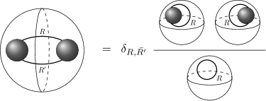
Figure 4: An illustration of the connected sum formula, applied to a network of Wilson lines in $S^{3}$ and a separating 2-sphere $S^{2}$ that cuts the network at two Wilson lines in representations $R$ and $R^{\prime}$. When $R\cong\overline{R}^{\prime}$, its partition function factorizes into contributions from the Wilson line networks in the left and right hemisphere, respectively, where the $R$ and $R^{\prime}=\overline{R}$ Wilson lines are joined.

Framing and skein relations

Surgeries other than a simple connected sum enable us to study braiding of Wilson lines, skein relations, and to compute the expectation values of Wilson loops colored by various representations. In general, given a surgery presentation of $M_{3}$, we can compute the expectation values of Wilson line operators in it by the surgery formula [25].

Figure 5: Wilson lines with extra twists.

The simplest example is the relation among twisted Wilson lines. The path integral on a $3$-ball containing a straight Wilson line in some representation $R$ ending on the boundary $2$-sphere determines a vector in the one-dimensional Hilbert space ${\mathcal{H}}_{S^{2}\{R,\overline{R}\}}$. This is also true when the Wilson line has extra twists, as in Figure 5. In particular, the vectors associated to Wilson lines with different number of twists are proportional. Assuming vertical framing, the Wilson lines in Figure 5 are related by $(\pm 1)$-Dehn twists on the boundary $2$-sphere. The proportionality constant in this case is $e^{2\pi ih_{R}}$ where $h_{R}$ is the conformal weight of the primary field of the WZW model transforming in representation $R$.

Figure 6: Skein relation of vertically framed Wilson lines in the fundamental representation $\square$.

In a similar fashion one obtains skein relations. Consider a $3$-ball with two Wilson lines labeled by the fundamental representation $\square$, ending on the boundary $2$-sphere. The associated Hilbert space ${\mathcal{H}}_{S^{2},\{\square,\square,\overline{\square},\overline{\square}\}}$ is two-dimensional, so the three configurations of Wilson lines in Figure 6 have to satisfy a linear relation. The coefficients of this relation can be determined from the fact that the configurations are related by half-twists on the boundary $2$-sphere, c.f. [25, 26]. In Figure 6 we expressed them in terms of the variable

$$q=e^{\pi i/(N+\kappa)}\,.$$ (10)

Note that the exact form of the relation depends on the choice of framing. We use the vertical framing throughout this paper, which is why the skein relation here looks different from its more familiar form in the canonical framing, in which the coefficients of the first two terms are $q^{-N}$ and $-q^{N}$, respectively. A thorough discussion of this can be found in [26].

Next, let us show how to obtain the expectation value of an unknotted Wilson loop in $S^{3}$ labeled by an irreducible representation $R_{i}$. The idea is that such a configuration can be obtained by Dehn surgery on $S^{2}\times S^{1}$, with the Wilson line running along the $S^{1}$. More precisely, let $M_{3}$ be a tubular neighborhood of the Wilson line in $S^{2}\times S^{1}$, and $M_{3}^{\prime}$ its complement. Then $S^{3}$ can be obtained by gluing $M_{3}$ and $M_{3}^{\prime}$ along the boundary torus $T^{2}$, with a non-trivial identification by the global diffeomorphism $S\in SL(2,{\mathbb{Z}})$:

$${\mathcal{Z}}(S^{3},R_{i})={}_{T^{2}}\langle M_{3}^{\prime}|S|M_{3},R_{i}\rangle_{T^{2}}\,.$$ (11)

Here we use the crucial fact that the mapping class group of $T^{2}$ acts on ${\mathcal{H}}_{T^{2}}$ by the modular transformation on the characters of the respective Kac-Moody algebra. In particular,

$$S|M_{3},R_{i}\rangle_{T^{2}}=\sum_{j}S_{ij}|M_{3},R_{j}\rangle_{T^{2}}\,,$$ (12)

where $S_{ij}$ is the modular $S$-matrix. Hence,

$${\mathcal{Z}}(S^{3},R_{i})=\sum_{j}S_{ij}\;{}_{T^{2}}\langle M_{3}^{\prime}|M_{3},R_{j}\rangle_{T^{2}}=\sum_{j}S_{ij}\;{\mathcal{Z}}(S^{2}\times S^{1},R_{j})\,,$$ (13)

but ${\mathcal{Z}}(S^{2}\times S^{1},R_{j})={\rm tr}_{{\mathcal{H}}_{S^{2}\{R_{j}\}}}(1)={\rm dim}({{\mathcal{H}}_{S^{2}\{R_{j}\}}})$, which is $1$ if $R_{j}$ is the trivial representation and $0$ otherwise. It immediately follows that the expectation value of a Wilson loop in $S^{3}$ is given by the quantum dimension

$$\langle W_{R_{j}}\rangle_{S^{3}}={{\mathcal{Z}}(S^{3},R_{i})\over{\mathcal{Z}}(S^{3},R_{0}={\rm triv})}={S_{i0}\over S_{00}}\,.$$ (14)

For Wilson lines in the totally antisymmetric representations in $SU(N)$ Chern-Simons theory at level $\kappa$, this gives

$$\langle W_{\wedge^{m}\square}\rangle=\dfrac{S_{0,\wedge^{m}\square}}{S_{0,0}}={N\brack m}\,,$$ (15)

where

$${N\brack m}=\dfrac{[N]\cdots[N-m+1]}{[m]\cdots[1]}\,,\quad\left[N\right]=\dfrac{q^{N}-q^{-N}}{q-q^{-1}}\,$$ (16)

is the quantum binomial coefficient.

Tetrahedral network and normalization of trivalent vertices

Figure 7: The evaluation of a “$\theta$-web” that determines the normalization of the vertices $\epsilon$ and $\widetilde{\epsilon}$. Here $k$ stands for a totally antisymmetric representation $\wedge^{k}\square$.

As we explained earlier, there are only two possible trivalent junctions between Wilson lines in totally antisymmetric representations, c.f. Figure 3(b). Moreover, the spaces of junction fields

$$\epsilon \in \text{Hom}(\Lambda^{k_{1}+k_{2}}\square,\Lambda^{k_{1}}\square\otimes\Lambda^{k_{2}}\square)\,,$$ (17)

$$\widetilde{\epsilon} \in \text{Hom}(\Lambda^{k_{1}}\square\otimes\Lambda^{k_{2}}\square,\Lambda^{k_{1}+k_{2}}\square)$$

are each one-dimensional. We choose $\epsilon$ and $\widetilde{\epsilon}$ as positive multiples of the respective antisymmetrizations of the identity maps $\square^{k_{1}}\otimes\square^{k_{2}}\longleftrightarrow\square^{k_{1}+k_{2}}$. Note that this choice depends on the ordering of $(k_{1},k_{2})$, where a change of the ordering leads to a sign factor $(-1)^{k_{1}k_{2}}$. The normalization is fixed by requiring the relation in Figure 7 to hold. Note that this differs from the normalization used in [26], where the “$\theta$-web” would evaluate to $\sqrt{{N\brack k_{1}}{N\brack k_{2}}{N\brack k_{1}+k_{2}}}$.

Figure 8: Relations between vertices in the conventions of [26]. Our choice for the vertices between totally antisymmetric representations $\Lambda^{k_{1}}\square$, $\Lambda^{k_{2}}\square$ and $\Lambda^{k_{1}+k_{2}}\square$ involves an extra sign factor $(-1)^{k_{1}k_{2}}$.

Also, our choice of signs leads to an additional factor of $(-1)^{k_{1}k_{2}}$ in the vertex relations depicted in Figure 8, which are valid in the conventions of [26], when $a,b,c$ are totally antisymmetric representations $\Lambda^{k_{1}}\square$, $\Lambda^{k_{2}}\square$ and $\Lambda^{k_{1}+k_{2}}\square$.

Figure 9: Evaluation of the tetrahedral web.

We conclude this review by computing the expectation value of the tetrahedral network in Figure 9. It has four Wilson lines in antisymmetric representations $\wedge^{k}\square,\wedge^{k}\square,\wedge^{k+1}\square,\wedge^{k-1}\square$ and two diagonal Wilson lines in the fundamental $\square$, which are positively crossed. The braiding relations for vertices (c.f. Figure 8) on the two junctions at the end of a diagonal line, imply that the expectation value of this tetrahedron is proportional to the expectation value of the one, in which the fundamental Wilson lines are negatively crossed. The constant of proportionality can be easily calculated to be $q^{-2-\frac{2}{N}}$. (The relevant conformal weights satisfy $\exp(2\pi i\,h(\Lambda^{k}\square))=q^{(1+\frac{1}{N})(N-k)k}$.) Using the skein relation of Figure 6 one arrives at the first equation in Figure 9. The second equality follows from the connected sum formula (Figure 4).

2.2 Web relations

Figure 10: Relations among networks of Wilson lines.

Networks of Wilson lines in totally antisymmetric representations satisfy the linear relations depicted in Figure 10. These relations have interesting implications. For instance, identities (e) and (f) are part of the defining relations of the quantum group $\dot{\mathbf{U}}_{q}(\mathfrak{sl}_{m})$. The connection between Wilson lines and quantum groups is the subject of section 2.3 below. Here, we will demonstrate how to derive such relations using the one in Figure 10(e) as an example. The proofs of the other relations are deferred to Appendix A.

Consider the three configurations of Wilson lines in Figure 10(e) (all lying in $3$-balls with ends on the boundary $2$-sphere). The path integral in these systems gives three vectors in ${\mathcal{H}}_{S^{2},\{m,j,\overline{m},\overline{j}\}}$. Since the dimensions of this space is greater than $2$ for general $m$ and $j$, it is not a priori clear that a relation we are seeking exists. In order to obtain it, we start with the relations among networks in Figure 11(a).

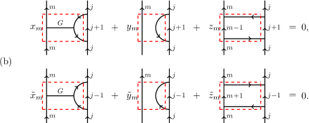
Figure 11: (a) Two linear relations among three Wilson lines in ${\mathcal{H}}_{S^{2},\{1,m,\overline{1},\overline{m}\}}$, (b) two linear relations among three Wilson lines containing those of (a) in the red dashed box, and (c) proportionality relations between two vectors in ${\mathcal{H}}_{S^{2},\{G,j,\overline{j}\}}$.

That such relations (with some coefficients) have to hold follows from the fact that ${\mathcal{H}}_{S^{2},\{1,m,\overline{1},\overline{m}\}}$ is $2$-dimensional. Here, $G$ stands for the adjoint representation, and we have chosen non-trivial vertices at the end-points of the Wilson lines colored by $G$. (In fact, ${\mathcal{H}}_{S^{2},\{G,m,\overline{m}\}}$ is one-dimensional, so the gauge invariant tensor lying at the junction of $G,m,\overline{m}$-colored Wilson lines is proportional to the multiplication $G\otimes\wedge^{m}\square\rightarrow\wedge^{m}\square$. Nevertheless, the precise normalization need not be specified, since as long as $x_{m}$ and $\widetilde{x}_{m}$ in Figure 11(a) are nonzero, we will eventually get Figure 12. That $x_{m}$ and $\widetilde{x}_{m}$ are nonzero can be easily shown by closing off the Wilson lines of Figure 11(a) in two inequivalent ways.) Inserting these relations into larger networks of Wilson lines leads to relations of Figure 11(b).

Next, from $1$-dimensionality of ${\mathcal{H}}_{S^{2},\{G,j,\overline{j}\}}$ one derives the relations in Figure 11(c). (Again, we have chosen non-trivial junction fields.) This allows us to relate the first two terms in the identities of Figure 11(b), and hence to eliminate them from the relations. One arrives at the new relation depicted in Figure 12, which is a linear relation of the type we are after. To deduce (e) of Figure 10, it remains to determine the coefficients $\alpha$ and $\beta$.

Figure 12: A linear relation among three vectors in $\mathcal{H}_{S^{2},\{j,m,\overline{j},\overline{m}\}}$. The coefficients $\alpha$ and $\beta$ are functions of $x_{m},y_{m},z_{m},\widetilde{x}_{m},\widetilde{y}_{m},\widetilde{z}_{m},\eta_{j},\eta^{\prime}_{j}$.

We will do this in two steps. First we close off the $m$- and $j$-colored Wilson lines in Figure 12. Using the expectation values of all the resulting networks of Wilson lines that have been determined earlier we obtain the following relation

$$\left[N\right]=\alpha\left[N-j\right]\left[m\right]-\beta\left[N-m\right]\left[j\right]\,.$$ (18)

Another relation can be found by connecting the incoming $m$- and $j$-colored Wilson lines in Figure 12 with a junction to an incoming $j+m$ Wilson line. Since ${\mathcal{H}}_{S^{2},\{j,m,\overline{j+m}\}}$ is one-dimensional, the vectors associated to all three configurations of Wilson lines are proportional to one another. The constants of proportionality can be easily found: close off Wilson lines in relation of Figure 10(a) in a way shown in Figure 13(a), then insert the identity of Figure 10(b), and finally apply the resulting identity twice. The result is depicted in Figure 13(b), from which we obtain another relation on the coefficients $\alpha$ and $\beta$:

$$1=\alpha\left[m\right]\left[j+1\right]-\beta\left[m+1\right]\left[j\right]\,.$$ (19)

Together with (18) this fixes the sought-after coefficients to be

$$\frac{1}{\alpha}=\left[m-j\right]=\frac{1}{\beta}\,,$$ (20)

finally proving the relation of Figure 10(e).

Let us conclude this subsection by adding a remark on the expectation values of closed and planar trivalent graphs $\Gamma$ of Wilson lines. The relations in Figure 10, together with the expectation value of the Wilson loops (equation 15), form the complete set of Murakami-Ohtsuki-Yamada (MOY) graph polynomial relations which uniquely determines the MOY graph polynomials $P_{N}(\Gamma;q)\in{\mathbb{Z}}[q,q^{-1}]$, see [28]. As the MOY graphs are closed, oriented graphs generated by the junctions of Figure 3(b), the uniqueness theorem implies that the expectation value of any planar Wilson lines in antisymmetric representations (and their junctions) can be computed from the definition of MOY graph polynomials. This not only provides us a consistency check for our methods, but also a combinatorial way to compute the expectation value of networks of Wilson lines, as the MOY graph polynomials are combinatorially defined.

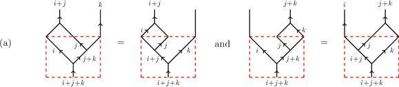
Figure 13: (a) Capping off the “associativity identity”. (b) Relations in ${\mathcal{H}}_{S^{2},\{j,m,\overline{j+m}\}}$.

2.3 Skew Howe duality and the quantum group

The quantum group ${\mathbf{U}}_{q}(\mathfrak{sl}_{2})$ is usually defined by means of generators $E,F,K,K^{-1}$ and relations (1). In finite dimensional representations of ${\mathbf{U}}_{q}(\mathfrak{sl}_{2})$, $K$ can be diagonalized with eigenvalues $q^{n}$, here $n\in{\mathbb{Z}}$ is the respective $\mathfrak{sl}_{2}$-weight. $E$ and $F$ raise, respectively lower the weights by $2$. For such representations, one can trade the generators $K,K^{-1}$ for idempotents $1_{n}$, $n\in{\mathbb{Z}}$, projecting on weight spaces of weight $n$

$$1_{n}1_{m}=\delta_{n,m}1_{n}\,.$$ (21)

This leads [4] to a modified quantum group $\dot{\mathbf{U}}_{q}(\mathfrak{sl}_{2})$ generated by $E,F$ and the $1_{n}$. Since $K1_{n}=q^{n}1_{n}$, the algebra relations become

$$E1_{n}=1_{n+2}E=1_{n+2}E1_{n}\,,\qquad F1_{n}=1_{n-2}F=1_{n-2}F1_{n}$$ (22)

$$\left[E,F\right]1_{n}=\left[n\right]1_{n}\,.$$

It is now very easy to see that if we identify

$$1_{k_{2}-k_{1}}\;\mapsto\;\,\begin{array}[]{c}\\ \begin{picture}(30.0,55.0)\put(0.0,10.0){\vector(0,1){35.0}} \put(0.0,45.0){\line(0,1){10.0}} \put(-3.0,0.0){${\scriptstyle k_{1}}$} \put(25.0,10.0){\vector(0,1){35.0}} \put(25.0,45.0){\line(0,1){10.0}} \put(22.0,0.0){${\scriptstyle k_{2}}$} \end{picture}\end{array}\,,\qquad E\;\mapsto\;\,\begin{array}[]{c}\\ \begin{picture}(30.0,55.0)\put(0.0,10.0){\vector(0,1){15.0}} \put(0.0,25.0){\vector(0,1){20.0}} \put(0.0,45.0){\line(0,1){10.0}} \put(25.0,10.0){\vector(0,1){15.0}} \put(25.0,25.0){\vector(0,1){20.0}} \put(25.0,45.0){\line(0,1){10.0}} \put(0.0,32.0){\vector(1,0){15.0}} \put(15.0,32.0){\line(1,0){10.0}} \put(11.0,36.0){${\scriptstyle 1}$} \end{picture}\end{array}\,,\qquad F\;\mapsto\;\,\begin{array}[]{c}\\ \begin{picture}(30.0,55.0)\put(0.0,10.0){\vector(0,1){15.0}} \put(0.0,25.0){\vector(0,1){20.0}} \put(0.0,45.0){\line(0,1){10.0}} \put(25.0,10.0){\vector(0,1){15.0}} \put(25.0,25.0){\vector(0,1){20.0}} \put(25.0,45.0){\line(0,1){10.0}} \put(25.0,32.0){\vector(-1,0){15.0}} \put(0.0,32.0){\line(1,0){10.0}} \put(11.0,36.0){${\scriptstyle 1}$} \end{picture}\end{array}\,,$$ (23)

as in [3], then, upon concatenation, these configurations of Wilson lines satisfy the quantum group relations, (21) and (22). In particular, the commutation relation of $E$ and $F$ is nothing but the identity of Figure 10(e), which was explained in the previous subsection. Here, composition of webs (networks) is drawn from bottom to top, and Wilson lines with different labels cannot be joined, i.e. their concatenation vanishes. Note, that $E$ and $F$ do not change $k=k_{1}+k_{2}$, which characterizes the quantum group representation. For fixed $k$ the identification of strands and idempotents is unambiguous.

Interestingly, while it is well known that the quantum group ${\mathbf{U}}_{q}(\mathfrak{sl}_{N})$ appears in the description of $SU(N)$ Chern-Simons theories, here we realize the quantum group $\mathfrak{sl}_{2}$ in Chern-Simons theory with gauge group $SU(N)$ for any $N$. The choice of gauge group merely restricts the possible $\mathfrak{sl}_{2}$ weights which can appear. After all, the labels $k_{i}$ stand for totally antisymmetric representations $\Lambda^{k_{i}}\square$ in $SU(N)$ Chern-Simons theory. Hence, the $\mathfrak{sl}_{2}$ weights can only lie between $-N$ and $N$. The networks of Wilson lines in $SU(N)$ Chern-Simons theory therefore only realize quantum group representations with highest weights $\leq N$.

Figure 14: $\dot{\mathbf{U}}_{q}(\mathfrak{sl}_{m})$ idempotents and generators in terms of Wilson lines and their junctions.

This construction can easily be generalized by increasing the number of strands of Wilson lines to $m>2$. One defines idempotents $1_{\lambda}$, $\lambda=(k_{2}\!-\!k_{1},\cdots,k_{m}\!-\!k_{m-1})\in\mathbb{Z}^{m-1}$ by $m$ parallel strands of Wilson line with labels $k_{1},\ldots,k_{m}$. For $1\leq i\leq m$, the generators $E_{i}$ (resp. $F_{i}$) are defined by suspending a Wilson line in the fundamental representation between the $i$th and $(i+1)$st strand (resp. between the $(i+1)$st and the $i$th strand). These definitions are illustrated in Figure 14. Then, using in particular identities (e) and (f) of Figure 10, one finds that these webs satisfy the defining relations of the higher rank quantum group $\dot{\mathbf{U}}_{q}(\mathfrak{sl}_{m})$:

$$\begin{split}1_{\lambda}1_{\lambda^{\prime}}=\delta_{\lambda,\lambda^{\prime}}1_{\lambda},\quad E_{i}1_{\lambda}=1_{\lambda+l_{i}}E_{i},\quad F_{i}1_{\lambda}=1_{\lambda-l+i}F_{i},\\[6.45831pt] [E_{i},F_{j}]1_{\lambda}=\delta_{i,j}[\lambda_{i}]1_{\lambda},\quad[E_{i},E_{j}]1_{\lambda}=0\quad\text{for}\quad|i-j|>1,\\[6.45831pt] \text{and}\quad E_{i}E_{j}E_{i}1_{\lambda}=E_{i}^{(2)}E_{j}1_{\lambda}+E_{j}E_{i}^{(2)}1_{\lambda}\quad\text{for}\quad|i-j|=1.\end{split}$$ (24)

Here $\lambda$ denotes an $\mathfrak{sl}_{m}$ weight. The generators $E_{i}$ (resp. $F_{i}$) associated to the simple roots of $\mathfrak{sl}_{m}$ raise (resp. lower) $\lambda$ by $l_{i}=(0,\ldots,0,-1,2,-1,0,\ldots,0)$ where $2$ appears in position $i$.

To summarize, in $SU(N)$ Chern-Simons theory with arbitrary $N$, we obtain a realization of $\dot{\mathbf{U}}_{q}(\mathfrak{sl}_{m})$ on a configurations of Wilson lines with $m$ strands. The rank of the Chern-Simons gauge group only restricts the possible representations of the quantum group which can be obtained in this way. What we described is a physical realization of the skew Howe duality of [2]

$$\Lambda^{k}({\mathbb{C}}^{m}\otimes{\mathbb{C}}^{N})\cong\bigoplus_{k_{1}+\ldots+k_{m}=k}\Lambda^{k_{1}}{\mathbb{C}}^{N}\otimes\ldots\otimes\Lambda^{k_{m}}{\mathbb{C}}^{N}\,.$$ (25)

The actions of $\mathfrak{sl}_{m}$ and $\mathfrak{sl}_{N}$, respectively, on ${\mathbb{C}}^{m}$ and ${\mathbb{C}}^{N}$ commute, and the direct sum on the RHS of this equation is indeed the weight decomposition with respect to the $\mathfrak{sl}_{m}$ action. This duality has a direct generalization to quantum groups $\dot{\mathbf{U}}_{q}(\mathfrak{sl}_{m})$.

In Chern-Simons theory we interpret each summand on the RHS of (25) as the Hilbert space of $m$ Wilson lines in representations, $R_{1}=\Lambda^{k_{1}}{\mathbb{C}}^{N}$, etc.,

$$R_{1}\otimes\ldots\otimes R_{m}\;=\;\Lambda^{k_{1}}{\mathbb{C}}^{N}\otimes\ldots\otimes\Lambda^{k_{m}}{\mathbb{C}}^{N}\,,$$ (26)

so that raising and lowering operators, $E_{i}$ and $F_{i}$, which relate different weight spaces are realized as configurations of $SU(N)$ Wilson lines in totally antisymmetric representations with $m$ incoming and $m$ outgoing strands.

Figure 15: “Tag” morphism relation of the $N\rm{Web}$ category.

In fact, the identification of Figure 14 exactly corresponds to the skew Howe duality functor from the quantum group $\dot{\mathbf{U}}_{q}(\mathfrak{sl}_{m})$ to the category $N\rm{Web}_{m}$ [3], whose objects are tuples $(k_{1},\ldots,k_{m})$, $0\leq k_{i}\leq N$, and whose morphisms are “$\mathfrak{sl}_{N}$-webs”. The latter are generated by the morphisms depicted in Figure 14 modulo the relations of Figure 10.

Note that the category $N\rm{Web}_{m}$ contains a “tag” morphism satisfying the relation in Figure 15. This tag corresponds to a junction with the $N$th antisymmetric representation. Since this is a trivial representation, the respective Wilson line is trivial and does not have to be drawn. The junction however still requires a specification of the junction field, i.e. an invariant tensor $\Lambda^{k}\square\otimes\Lambda^{N-k}\square\longrightarrow\Lambda^{N}\square$, which was determined by the ordering of incoming Wilson lines. This ordering is specified by the direction of the outgoing Wilson line, hence the tag, and the change of ordering leads to a sign factor $(-1)^{k(N-k)}$ as in the tag relation.

2.4 Why “categorification = surface operators”

In general, a $d$-dimensional TQFT assigns a number (= partition function) to every closed $d$-manifold $M_{d}$, a vector space ${\mathcal{H}}(M_{d-1})$ to every $(d-1)$-manifold, a category $\mathfrak{C}(M_{d-2})$ to every $(d-2)$-manifold, and so on. Therefore, the process of “categorification” that promotes each of these gadgets to the higher categorical level has an elegant interpretation as “dimensional oxidation” in TQFT, which promotes a $d$-dimensional TQFT to a $(d+1)$-dimensional one [29] (see also [20]).

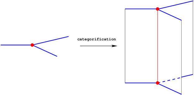
Figure 16: Categorification means lifting a given theory to one dimension higher. This operation of adding an extra dimension turns line operators into surface operators [20] and graphs (networks) into foams (surfaces with singular edges).

Many interesting theories come equipped with non-local operators (often called “defects”) that preserve and frequently ameliorate the essential structure of the theory. Categorification has a natural extension to theories with such non-local operators which also gain an extra dimension, much like the theory itself. Prominent examples of such operators are codimension-$2$ line operators in 3d Chern-Simons TQFT that we encountered earlier and that do not spoil the topological invariance of the theory. One dimension lower, such codimension-$2$ operators would actually be local operators supported at points $p_{i}$ on a 2-manifold $M_{2}$. And, one dimension higher, in a 4d TQFT such codimension-$2$ operators would be supported on surfaces $\Sigma\subset M_{4}$. Therefore, on general grounds a categorification of 3d Chern-Simons invariants should be a functor (4d TQFT) that assigns

$${\mbox{\rm surface}}~{}\Sigma\subset M_{4}\quad \leadsto \quad{\mbox{\rm number}}~{}Z(M_{4};\Sigma)$$

$${\mbox{\rm knot/web}}~{}K\subset M_{3}\quad \leadsto \quad{\mbox{\rm vector space}}~{}{\mathcal{H}}(M_{3};K)$$ (27)

$${\mbox{\rm points}}~{}p_{1},\ldots,p_{n}\in M_{2}\quad \leadsto \quad{\mbox{\rm category}}~{}\mathfrak{C}(M_{2};p_{1},\ldots,p_{n})$$

$$\vdots$$

In particular, as illustrated in Figure 16, categorification of graphs and networks is achieved by studying surface operators with singular edges (junctions) in four dimensions. This naturally leads us to the study of junctions of surface operators and the effective 2d theory on their world-sheet $\Sigma$ which, respectively, will be the subjects of sections 3 and 4.

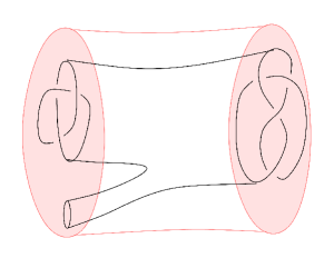
Figure 17: A link cobordism $\Sigma$ defines a map between the corresponding homology groups.

Moreover, functoriality implies that the structure at each level should be compatible with cobordisms as well as operations of cutting and gluing. It turns out to be very rich even before one tackles the very interesting question of studying tangle cobordisms in non-trivial ambient manifolds. In other words, even when $M_{2}={\mathbb{R}}^{2}$, $M_{3}={\mathbb{R}}^{3}$ and $M_{4}={\mathbb{R}}^{4}$ in (27) functoriality can be highly non-trivial due to interesting topologies of $K$ and $\Sigma$. In particular, a surface cobordism $\Sigma$ between links $K_{1}$ and $K_{2}$ gives rise to a linear map (see Figure 17):

$$Z(\Sigma)~{}:\quad{\mathcal{H}}(K_{1})\longrightarrow{\mathcal{H}}(K_{2})$$ (28)

where, to avoid clutter, we tacitly assumed that all components of $K_{1}$ and $K_{2}$ have the same color. (Otherwise, $\Sigma$ can not be a smooth surface and must be a foam, i.e. have singular edges.) In fact, all our defects — line operators in 3d, surface operators in 4d, as well as points in 2d — carry certain labels or colors which we denote by $R_{i}$. For example, making this part of our notation explicit and, on the other hand, suppressing $M_{2}={\mathbb{R}}^{2}$, the third line in (27) should read:

$$(p_{1},R_{1}),\ldots,(p_{n},R_{n})\quad\leadsto\quad{\mbox{\rm category}}~{}\mathfrak{C}_{R_{1},\ldots,R_{n}}$$ (29)

The Hochschild homology of this category must be the cohomology of $n$ copies of the unknot, colored by $R_{1},\ldots,R_{n}$, respectively:

$$HH^{*}(\mathfrak{C}_{R_{1},\ldots,R_{n}})\;=\;{\mathcal{H}}^{R_{1}}\big{(}{\,\raisebox{-2.27626pt}{\includegraphics[width=11.38092pt]{unknot}}\,}\big{)}\otimes\ldots\otimes{\mathcal{H}}^{R_{n}}\big{(}{\,\raisebox{-2.27626pt}{\includegraphics[width=11.38092pt]{unknot}}\,}\big{)}$$ (30)

This is a part of the reverse process, called “decategorification,” which in TQFT corresponds to dimensional reduction (of the “time” direction). It will prove very useful later, in section 4.2, where it will help us to better understand the cohomology of the colored unknot as well as the structure of the category (29). Notably, applying (28) to the cobordism between on the one hand the disjoint union $K_{1}=K\bigsqcup{\,\raisebox{-2.27626pt}{\includegraphics[width=11.38092pt]{unknot}}\,}$ of a knot $K$ with the unknot and on the other hand their connected sum $K_{2}=K\#{\,\raisebox{-2.27626pt}{\includegraphics[width=11.38092pt]{unknot}}\,}\cong K$ which gives back $K$, yields a map

$${\mathcal{A}}\otimes{\mathcal{H}}^{R}(K)\;\to\;{\mathcal{H}}^{R}(K)\,,$$ (31)

where

$${\mathcal{A}}\;:=\;{\mathcal{H}}^{R}({\,\raisebox{-2.27626pt}{\includegraphics[width=11.38092pt]{unknot}}\,})\,.$$ (32)

In fact, for the special case $K={\,\raisebox{-2.27626pt}{\includegraphics[width=11.38092pt]{unknot}}\,}$ this defines an algebra structure

$${\raisebox{-11.38092pt}{\includegraphics[width=28.45274pt]{cobordism1}}\,}~{}:\qquad{\mathcal{A}}\otimes{\mathcal{A}}\;\to\;{\mathcal{A}}\,,$$ (33)

on the homology of the unknot, and (31) promotes the homology ${\mathcal{H}}^{R}(K)$ of any knot $K$ to an ${\mathcal{A}}$-module.

It turns out that the algebra structure of the unknot homology (33) contains a lot of useful information about how the theory behaves under cobordisms [30, 31, 32] and has been used to construct various deformations of Khovanov-Rozansky homology [33, 34, 35, 36, 37, 38]. Much of this algebraic structure extends even to colored HOMFLY-PT homology [39].

A 2d TQFT is basically determined by a Frobenius algebra, defined by a “pair-of-pants” product as in (33). In case the theory is obtained from a supersymmetric one by topological twisting, than this algebra is the chiral ring of the untwisted theory. In our present context this implies that the chiral ring of the world-volume theory of a surface operator labeled by representation $R$ has to agree with the algebra (33) associated to the unknot colored by $R$,

$${\mathcal{A}}\;=\;{\mathcal{H}}^{R}({\,\raisebox{-2.27626pt}{\includegraphics[width=11.38092pt]{unknot}}\,})\;=\;\text{chiral ring of 2d TQFT on the surface operator}\,.$$ (34)

This provides a useful clue for identifying the surface operators (and their world-volume theories) which are relevant for the categorification of quantum groups.

For example, the original Khovanov homology [40] is based on the nilpotent Frobenius algebra

$${\mathcal{A}}\;=\;{\mathbb{C}}[X]/\langle X^{2}\rangle$$ (35)

A semi-simple deformation of this algebra studied by Lee [33] led to a number of important developments, including Rasmussen’s proof of the Milnor conjecture [41].

3 Junctions of surface operators

Surface operators are non-local operators which, in four-dimensional QFT, are supported on two-dimensional surfaces embedded in four-dimensional space-time $M_{4}$,

$$\Sigma\;\subset\;M_{4}$$ (36)

Intuitively, surface operators can be thought of as non-dynamical flux tubes (or vortices) much like Wilson and ’t Hooft line operators can be thought of as static electric and magnetic sources, respectively. Compared to line operators, however, surface operators have a number of peculiar features. See [42] for a recent review on surface operators.

Thus, in gauge theory with gauge group $G$, line operators are labeled by discrete parameters, namely electric and magnetic charges of the static source, while surface operators in general are labeled by both discrete and continuous parameters. The former are somewhat analogous to discrete labels of line operators, but the latter are a novel feature of surface operators.

In practice, there are two basic ways of constructing surface operators:

• as a singularity along $\Sigma$, e.g.

  $$F=2\pi\alpha\delta_{\Sigma}+\ldots$$ (37)

• as a coupled 2d-4d system, e.g. described by the action

  $$S_{\text{tot}}=\int_{M_{4}}d^{4}x\;\left({\mathcal{L}}_{\text{4d}}+\delta_{\Sigma}\cdot{\mathcal{L}}_{\text{2d}}\right)=\int_{M_{4}}d^{4}x\;{\mathcal{L}}_{\text{4d}}+\int_{\Sigma}d^{2}x\;{\mathcal{L}}_{\text{2d}}$$ (38)

  where the global symmetry $G$ of the 2d Lagrangian ${\mathcal{L}}_{\text{2d}}$ is gauged when coupled to the 4d Lagrangian ${\mathcal{L}}_{\text{4d}}$.

Both descriptions can be very useful for establishing the existence and analyzing junctions of surface operators, which locally look like a product of “time” direction ${\mathbb{R}}_{t}$ with a Y-shaped graph where three (or more) surface operators meet along a singular edge of the surface $\Sigma$, thus providing a physics home and a microscopic realization of the ideas advocated in [43, 44, 45]. A surface $\Sigma$ with such singular edges is often called a “foam” or a “seamed surface”.

Before one can start exploring properties of junctions and their applications, it is important to establish their existence at two basic levels:

$a)$ at the level of “kinematics” as well as

$b)$ at the level of field equations (or BPS equations, if one wants to preserve some supersymmetry).

The former means that junctions of surface operators must obey certain charge conservation conditions analogous to (6), while the latter means they must be a solution to field equations or BPS equations, at least classically. Addressing both of these questions will be the main goal of the present section, where we treat cases with different amount of supersymmetry in parallel. In particular, sections 3.1–3.4 will be devoted to the latter question, whereas kinematics will be largely the subject of section 3.5. Before we proceed to technicalities, however, let us give a general idea of what the answer to each of these questions looks like.

When a configuration of surface operator junctions is static, we have $\Sigma={\mathbb{R}}_{t}\times\Gamma$, where ${\mathbb{R}}_{t}$ is the “time” direction and $\Gamma$ is a planar trivalent graph or, more generally, a trivalent oriented graph in a 3-manifold $M_{3}$ which, for most of what we need in this paper, will be simply ${\mathbb{R}}^{3}$ (or $S^{3}$). Then, as we shall see, in many cases the BPS equations on $M_{3}$ will reduce to (or, at least, contain solutions of) the simple flatness equations for the gauge field $A$:

$$F_{A}\;=\;0$$ (39)

For example, the famous instanton equations $F_{A}^{+}=0$ in Donaldson-Witten theory reduce to (39) on a 4-manifold of the form ${\mathbb{R}}_{t}\times M_{3}$ when one requires solutions to be invariant under translations along ${\mathbb{R}}_{t}$. Since (39) is a “universal” part of BPS equations for many different systems, with different amounts of supersymmetry, it makes sense to illustrate how the questions of “kinematics” and the “existence of solutions” look in the case of (39). By doing so, we also focus our attention on the most interesting ingredient, namely the gauge dynamics. Then, adding more fields and interactions to the system is a relatively straightforward exercise and we comment on it in each case.

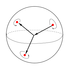
Figure 18: A small ball around a trivalent junction.

As explained in [19], a surface operator with non-zero $\alpha$ in (37) can be thought of as a Dirac string of a magnetic monopole with improperly quantized magnetic charge $\alpha$. Magnetic charges of monopoles that obey Dirac quantization condition take values in the root lattice $\Lambda_{\text{rt}}$ of the gauge group $G$. When this condition is not obeyed, the world-sheet of a Dirac string becomes visible to physics and this is precisely what a surface operator is. In this way of describing surface operator — as a singularity for the gauge field (and, possibly, other fields) — it should be clear that $\alpha$ in (37) takes values in the Lie algebra of the maximal torus of the gauge group, $\mathfrak{t}=\text{Lie}(\mathbb{T})$, modulo the lattice of magnetic charges $\Lambda_{\text{rt}}$. For example, when $G=U(1)$ the parameter $\alpha$ is a circle-valued variable.

In this description of a surface operator — as a singularity (37) or, equivalently, as a Dirac string of an improperly quantized magnetic charge — the orientation of the edges of the graph $\Gamma$ has a natural interpretation: it represents the magnetic flux. Of course, one can change the orientation of each edge and simultaneously invert the holonomy $U=\exp(2\pi i\alpha)\in G$ of the gauge field around it, without affecting the physics:

$$\xleftarrow[~{}~{}~{}~{}~{}~{}~{}~{}]{~{}U}\quad=\quad\xrightarrow[~{}~{}~{}~{}~{}~{}~{}~{}]{~{}U^{-1}}$$ (40)

Moreover, if the gauge field satisfies (39) away from the singularity locus $\Sigma={\mathbb{R}}_{t}\times\Gamma$, then the magnetic flux must be conserved at every junction. In the abelian theory with $G=U(1)$ it simply means that the signed sum (signs determined by the orientation) of the parameters $\alpha$ for all incoming and outgoing edges is equal to zero at every vertex of $\Gamma$, e.g.

$$\alpha=\alpha^{\prime}+\alpha^{\prime\prime}\quad(\text{mod}~{}1)$$ (41)

for a basic trivalent junction as depicted in Figure 18. A non-abelian version of flux conservation is more involved and will be discussed in section 3.5. This preliminary discussion, however, should give a reasonably good idea of what a junctions looks like in the description of a surface operator as a singularity (or, ramification) along $\Sigma$.

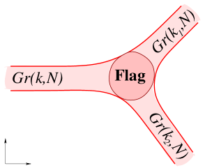
Figure 19: The core of a junction between surface operators (43) carries a partial flag variety $Fl(k_{1},N)$, $k=k_{1}+k_{2}$. Shown here is the $(x^{1},x^{2})$ plane.

Now, let us have a similar preliminary look at the same question from the viewpoint of a 2d-4d coupled system à la (38). In this approach, each face of the seamed surface $\Sigma$ is decorated with a 2d theory that lives on it, in many examples simply a 2d sigma-model with a target space ${\mathcal{C}}$ that enjoys an action of the symmetry group $G$, e.g. a conjugacy class or a flag variety ${\mathcal{C}}=G/\mathbb{L}$. In the approach based on 2d-4d coupled system, a junction of surface operators (or, a more general codimension-1 defect along $\Sigma$) determines a “correspondence” $\mathcal{M}\subset{\mathcal{C}}\times{\mathcal{C}}^{\prime}\times{\mathcal{C}}^{\prime\prime}$:

$$\begin{matrix}&&\mathcal{M}&&\\ &\swarrow&&\searrow&\\ {\mathcal{C}}&&&&{\mathcal{C}}^{\prime}\times{\mathcal{C}}^{\prime\prime}\end{matrix}$$ (42)

where ${\mathcal{C}}^{\prime}$ and ${\mathcal{C}}^{\prime\prime}$ are target spaces of 2d sigma-models on “incoming” edges of $\Gamma$ that join into an edge that carries sigma-model with target space ${\mathcal{C}}$. The description of such interfaces (or line defects) in the dual Landau-Ginzburg model will be the main subject of section 4.

Surface operators that will be relevant to skew Howe duality and categorification of quantum groups are labeled by “Levi types” $\mathbb{L}=S(U(k)\times U(N-k))$ in a theory with gauge group $G=SU(N)$, or simply by $k\in\{1,\ldots,N-1\}$. In the 2d-4d description of such “$k$-colored” surface operators the target space ${\mathcal{C}}=G/\mathbb{L}$ is the Grassmannian of $k$-planes in ${\mathbb{C}}^{N}$,

$${\mathcal{C}}\;=\;Gr(k,N)\;=\;SU(N)/S(U(k)\times U(N-k))$$ (43)

As we proceed, we will encounter Grassmannian varieties more and more often, as moduli spaces of solutions in gauge theory (later in this section) as well as in the description of interfaces and chiral rings in Landau-Ginzburg models (in section 4).

What about junctions of surface operators that carry Grassmannian sigma-model on their world-sheet? They can be conveniently described as correspondences (42), where ${\mathcal{M}}$ is a partial flag variety $Fl(k_{1},k,N)$ of $k_{1}$-planes in $k=(k_{1}+k_{2})$-planes in ${\mathbb{C}}^{N}$, as illustrated in Figure 19:

$$\begin{array}[]{ccccc}Gr(k,N)&\longleftarrow&Fl(k_{1},k,N)&\longrightarrow&Gr(k_{1},N)\times Gr(k_{2},N)\\ V&\mathrel{\reflectbox{$\longmapsto$}}&(V_{1}\subset V)&\longmapsto&(V_{1},V_{1}^{\perp}\subset V)\end{array}$$ (44)

Now, once we had a preliminary discussion of how the decorations of surface operators flow across junctions, both from the singularity perspective and in the approach of 2d-4d coupled system, it is natural to tackle the question of their existence at the level of field equations. As we already noted earlier, it involves solving PDEs in three dimensions with prescribed boundary conditions around $\Gamma\subset M_{3}$, which in general is not an easy task, even for the basic version of the equations (39). While it would be extremely interesting to pursue the construction of explicit solutions, we will only need to know whether they exist and what their moduli space looks like. Luckily, this latter question can be addressed without constructing explicit solutions and an illuminating way to do that is via embedding the gauge theory into string / M-theory.

Many interesting SUSY field theories on $M_{4}$ can be realized on stacks of M-theory fivebranes, such as configurations of

$$N~{}\text{M5-branes}\;{\rm on}\;M_{4}\times C$$ (45)

Indeed, for different choices of $2$-manifolds $C$ and their embeddings in the eleven-dimensional space-time one can realize 4d field theories on $M_{4}$ with ${\mathcal{N}}=1$, ${\mathcal{N}}=2$, or ${\mathcal{N}}=4$ supersymmetry. Below we consider each of these choices in turn.

In such constructions, one can “engineer” surface operators by introducing additional M5-branes or M2-branes which share only the two-dimensional part of the 4d geometry, $\Sigma\subset M_{4}$, with the original set of fivebranes (45). In particular, in such brane constructions, the junctions of surface operators relevant to skew Howe duality and categorification of quantum groups have a simple interpretation where one stack of $k$ branes splits up into two stacks of $k_{1}$ and $k_{2}=k-k_{1}$ branes, as illustrated in Figure 20.

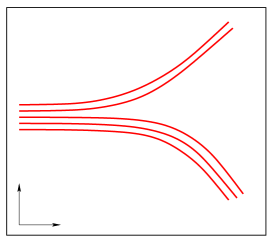
Figure 20: Brane realization of the junction of surface operators in Figure 19.

3.1 Junctions in 4d ${\mathcal{N}}=4$ theory

When $C=T^{2}$ or ${\mathbb{R}}^{2}$, the fivebrane configuration (45) preserves maximal (${\mathcal{N}}=4$) supersymmetry in 4d space-time $M_{4}$. Then, depending on the geometry of $\Sigma$ and $M_{4}$ in (36), one finds different fractions of unbroken supersymmetry.

If both $M_{4}$ and $\Sigma$ are flat, i.e. $M_{4}={\mathbb{R}}^{4}$ and $\Sigma={\mathbb{R}}^{2}$, then surface operators can be half-BPS and admit the following brane construction

$$\begin{array}[]{l@{\;}|@{\;}ccccccccccc}&~{}0{}&~{}1{}&~{}2{}&~{}3{}&~{}4{}&~{}5{}&~{}6{}&~{}7{}&~{}8{}&~{}9{}&~{}10{}\\ \hline\cr\text{M5}{}&\times&\times&\times&\times&&&\times&&&&\times\\ \text{M5}^{\prime}{}&\times&\times&&&&&\times&&\times&\times&\times\end{array}$$ (46)

where, following conventions of [48], we assume that $M_{4}$ is parametrized by $(x^{0},x^{1},x^{2},x^{3})$ and $C$ is parametrized by $x^{6}$ and $x^{10}$.

The half-BPS surface operators in 4d ${\mathcal{N}}=4$ theory can form $\frac{1}{4}$-BPS junctions of the form $\Sigma={\mathbb{R}}_{t}\times\Gamma$, where ${\mathbb{R}}_{t}$ is the $x^{0}$ “time” direction and $\Gamma$ is an arbitrary trivalent graph in the $(x^{1},x^{2})$-plane. In fact, without breaking supersymmetry further, we can take the 4d space-time to be $M_{4}={\mathbb{R}}_{t}\times M_{3}$, with an arbitrary 3-manifold $M_{3}$ locally parametrized by $(x^{1},x^{2},x^{3})$, and a knotted trivalent graph $\Gamma\subset M_{3}$. This requires partial topological twist of the 4d ${\mathcal{N}}=4$ theory along $M_{3}$, which in the brane construction (46) is realized by replacing the space ${\mathbb{R}}^{3}$ parametrized by $(x^{7},x^{8},x^{9})$ with the cotangent bundle to $M_{3}$.

Then, M5-branes are supported on ${\mathbb{R}}^{3}\times M_{3}$, while M5^′-branes are supported on ${\mathbb{R}}^{3}\times L_{\Gamma}$, where $M_{3}$ and $L_{\Gamma}$ are special Lagrangian submanifolds in a local Calabi-Yau space $T^{*}M_{3}$, such that

$$L_{\Gamma}\cap M_{3}=\Gamma$$ (47)

This configuration of fivebranes preserves 4 real supercharges, i.e. a quarter of the original ${\mathcal{N}}=4$ SUSY.

When $C=T^{2}$ or ${\mathbb{R}}^{2}$, we can consider a further generalization in which junctions of surface operators are not necessarily static. Such configurations preserve only 2 real supercharges — namely, ${\mathcal{N}}=(0,2)$ supersymmetry along $C$ — and recently have been studied [39, 49] in a closely related context. In particular, one can combine the time direction with $M_{3}$ into a general $4$-manifold $M_{4}$ and take $\Sigma$ to be an arbitrary surface (36) with singular trivalent edges, i.e. a foam or a seamed surface [44, 45].

For generic $\Sigma$, such foams or non-static junctions of surface operators will break supersymmetry unless we extend the partial topological twist along $M_{3}$ to all of $M_{4}$. In the fivebrane system (46) this twist is realized by replacing $(x^{7},x^{8},x^{9})$-directions with a non-trivial bundle over $M_{4}$, namely the bundle of self-dual 2-forms:

space-time: $$\qquad\Lambda^{2}_{+}(M_{4})\times{\mathbb{R}}^{4}$$

$$N \qquad~{}~{}~{}~{}~{}~{}M_{4}\times{\mathbb{R}}^{2}$$ M5-branes: (48)

$$k \qquad~{}~{}~{}~{}~{}~{}L_{\Sigma}\times{\mathbb{R}}^{2}$$ M5^′-branes:

where, much as in (47), $L_{\Sigma}$ and $M_{4}$ are coassociative submanifolds in a local $G_{2}$-holonomy manifold $\Lambda^{2}_{+}(M_{4})$, such that

$$L_{\Sigma}\cap M_{4}=\Sigma$$ (49)

As we already stated earlier, this generic configuration of surface operators preserves only 2 real supercharges (which, moreover, are chiral from the 2d perspective of $x^{6}$ and $x^{10}$).

3.2 Line-changing operators in class ${\mathcal{S}}$ and network cobordisms

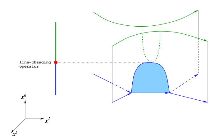
Figure 21: 6d fivebrane theory on a $2$-manifold $M_{2}$ parametrized by $x^{1}$ and $x^{2}$ yields 4d ${\mathcal{N}}=2$ theory $T[M_{2}]$ in the remaining four dimensions. In this theory, a network of line defects on $M_{2}$ determines a BPS line operator, whereas a “time evolution” of such network corresponds to segments of different line operators joined together at those values of “time” $x^{0}$ where the topology of network changes.

The intersection of M5-branes with M5^′-branes produces the so-called codimension-2 defect in the 6d $(0,2)$ theory on the fivebrane world-volume (45). The latter also admits codimension-4 defects which too can be used to produce surface operators in 4d theory on $M_{4}$ and which in M-theory are realized by M2-branes ending on M5-branes:

$$\begin{array}[]{l@{\;}|@{\;}ccccccccccc}&~{}0{}&~{}1{}&~{}2{}&~{}3{}&~{}4{}&~{}5{}&~{}6{}&~{}7{}&~{}8{}&~{}9{}&~{}10{}\\ \hline\cr\text{M5}{}&\times&\times&\times&\times&&&\times&&&&\times\\ \text{M2}{}&\times&\times&&&&&&\times&&&\end{array}$$ (50)

where the M2-brane world-volume is $\Sigma\times{\mathbb{R}}_{+}$, with ${\mathbb{R}}_{+}=\{x^{7}\geq 0\}$. In this realization of surface operators, BPS junctions can be obtained by considering codimension-4 defect supported on $\Sigma={\mathbb{R}}_{t}\times\Gamma$. In fact, let $M_{4}={\mathbb{R}}_{t}\times M_{2}\times{\mathbb{R}}$, where the $2$-manifold $M_{2}$ is a Riemann surface (possibly with punctures); this requires a partial topological twist of the fivebrane theory which, similar to (48), is realized by embedding $M_{2}$ in the space-time $T^{*}M_{2}$. Also, let $\Gamma\subset M_{2}$ be a colored trivalent graph on $M_{2}$ without self-intersections:

$$\begin{matrix}{\mbox{\rm 6d (0,2) theory:}}&\qquad&{\mathbb{R}}_{t}&\times&M_{2}&\times&{\mathbb{R}}&\times&C\\ &\qquad&\|&&\cup\\ {\mbox{\rm surface operator:}}&\qquad&{\mathbb{R}}_{t}&\times&\Gamma&&&&\end{matrix}$$ (51)

If we apply this to $C={\mathbb{R}}^{2}$ (or $C=T^{2}$), as in section 3.1, it is natural to ask what this configuration looks like from the viewpoint of ${\mathbb{R}}_{t}\times{\mathbb{R}}\times C\cong{\mathbb{R}}_{t}\times{\mathbb{R}}^{3}$, after compactification on the Riemann surface $M_{2}$. Due to partial topological twist along $M_{2}$, the resulting 4d theory $T[M_{2}]$ has only ${\mathcal{N}}=2$ supersymmetry and the codimension-$4$ defect (51) produces a line operator in this theory labeled by a colored trivalent network $\Gamma\subset M_{2}$.

This is precisely the configuration recently used in [50, 51, 52, 53, 54] to study line operators in 4d ${\mathcal{N}}=2$ theories $T[M_{2}]$. In our application here, we simply wish to interpret the Riemann surface $M_{2}$ as part of the 4d space-time. Then, the same configuration (51) describes “static” surface operators in 4d ${\mathcal{N}}=4$ theory on $M_{4}={\mathbb{R}}_{t}\times M_{2}\times{\mathbb{R}}$. Non-static surface operators correspond to networks $\Gamma(t)$ which vary with $t\in{\mathbb{R}}_{t}$; from the viewpoint of 4d ${\mathcal{N}}=2$ theory $T[M_{2}]$ they correspond to segments of different line operators glued together in a single line via local operators supported at those points $t_{i}\in{\mathbb{R}}_{t}$ where the network $\Gamma(t)$ changes topology. (Recall, that due to partial topological twist along $M_{2}$ only topology of the network $\Gamma$ matters.)

In other words, basic topological moves on $\Gamma$ realized via cobordisms correspond to line-changing operators in 4d ${\mathcal{N}}=2$ theory $T[M_{2}]$:

$$\text{network cobordism}\qquad\Leftrightarrow\qquad\text{line-changing operator}$$ (52)

Turning on Omega-background in 4d ${\mathcal{N}}=2$ theory $T[M_{2}]$ corresponds to replacing $C={\mathbb{R}}^{2}$ with $C={\mathbb{R}}^{2}_{\epsilon}$. This is precisely the setup we will use in application to knot homologies and categorification of quantum groups, cf. (101).

3.3 Junctions in 4d ${\mathcal{N}}=2$ theory

When $C$ is an arbitrary Riemann surface (possibly with boundaries and punctures) of genus $g\neq 1$, in order for the fivebrane configuration (45) to preserve supersymmetry its world-volume theory must be (partially) twisted along $C$. For the embedding of the fivebrane world-volume in the ambient space-time the partial topological twist means that $C$ must be either a holomorphic Lagrangian submanifold in a Calabi-Yau $2$-fold (that locally, near $C$ always looks like $T^{*}C$) or a holomorphic curve in a Calabi-Yau $3$-fold. The first choice preserves ${\mathcal{N}}=2$ supersymmetry in the 4d theory on $M_{4}$, while the second option preserves only ${\mathcal{N}}=1$ SUSY and will be considered next.

Consistent with (46), our choice of coordinates is

$$\begin{array}[]{c|c|c}M_{4}&T^{*}C&{\mathbb{R}}^{3}\\ \hline\cr~{}x^{0},~{}x^{1},~{}x^{2},~{}x^{3}{}&~{}x^{4},~{}x^{5},~{}x^{6},~{}x^{10}{}&~{}x^{7},~{}x^{8},~{}x^{9}{}\\ \end{array}$$ (53)

In particular, the $U(1)_{r}\times SU(2)_{R}$ R-symmetry group in this setup is identified with the $U(1)_{45}\times SU(2)_{789}$ symmetry of the eleven-dimensional geometry. When both $M_{4}={\mathbb{R}}^{4}$ and $\Sigma={\mathbb{R}}^{2}$ are flat, we can still use brane configuration (46) to describe half-BPS surface operators, this time in 4d ${\mathcal{N}}=2$ theory on $M_{4}$.

Also, as in the ${\mathcal{N}}=4$ case, we can describe junctions by taking $M_{4}={\mathbb{R}}_{t}\times M_{3}$ and replacing $(x^{7},x^{8},x^{9})$ with the cotangent bundle to $M_{3}$:

space-time: $$\qquad{\mathbb{R}}_{t}\times T^{*}M_{3}\times T^{*}C$$

$$N \qquad{\mathbb{R}}_{t}\times~{}M_{3}~{}\times~{}C$$ M5-branes: (54)

$$k \qquad{\mathbb{R}}_{t}\times~{}L_{\Gamma}~{}\times~{}C$$ M5^′-branes:

where, as in (47), $L_{\Gamma}$ and $M_{3}$ are special Lagrangian submanifolds in $T^{*}M_{3}$ which intersect over a knotted trivalent graph $\Gamma\subset M_{3}$. Then, the resulting brane configuration (54) describes junctions of half-BPS surface operators supported on a surface $\Sigma={\mathbb{R}}_{t}\times\Gamma$.

Due to the partial topological twist along $M_{3}$, the latter can be an arbitrary $3$-manifold and $\Gamma$ can be an arbitrary knotted graph. The price to pay for it is that junctions (54) preserve only $2$ real supercharges, i.e. again are $\frac{1}{4}$-BPS in the original 4d theory on $M_{4}$.

3.4 Junctions in 4d ${\mathcal{N}}=1$ theory

Even though 4d ${\mathcal{N}}=1$ theories are not directly related to the main subject of our paper, here for completeness we consider possible junctions of surface operators in such theories.

First, in a typical brane construction [55] of 4d ${\mathcal{N}}=1$ theories, $C$ is embedded as a holomorphic curve in a local Calabi-Yau $3$-fold:

$$M_{4}\times CY_{3}\times{\mathbb{R}}$$ (55)

This leaves little room for surface operators. In fact, even when $M_{4}={\mathbb{R}}^{4}$ this system admits a half-BPS surface operator that breaks supersymmetry down to ${\mathcal{N}}=(0,2)$ along $\Sigma={\mathbb{R}}^{2}$.

In the fivebrane construction (45) of the 4d ${\mathcal{N}}=1$ theory, this half-BPS surface operator can be realized by an additional system of M5^′-branes supported on a holomorphic $4$-cycle $D\subset CY_{3}$:

space-time: $$\qquad M_{4}\times CY_{3}\times{\mathbb{R}}$$

$$N \qquad M_{4}\times~{}C$$ M5-branes: (56)

M5^′-branes: $$\qquad~{}\Sigma~{}\times~{}D$$

Equivalently, via a “brane creation” phase transition [56], one can represent half-BPS surface operators in 4d ${\mathcal{N}}=1$ theory by M2-branes with a semi-infinite extent in the $x^{7}$-direction ($x^{7}\geq 0$):

space-time: $$\qquad M_{4}\times CY_{3}\times{\mathbb{R}}$$

$$N \qquad M_{4}\times~{}C$$ M5-branes: (57)

M2-branes: $$\qquad~{}\Sigma~{}\times\{\text{pt}\}\times{\mathbb{R}}_{+}$$

It is easy to verify that ${\mathcal{N}}=1$ supersymmetry on $M_{4}$ is not sufficient to allow for non-trivial BPS junctions of surface operators.

3.5 OPE of surface operators and the Horn problem

In non-abelian theory, the analogue of the flux conservation (41) is known as the multiplicative Horn problem:

$$\text{What conjugacy classes are contained in}~{}{\mathcal{C}}^{\prime}\cdot{\mathcal{C}}^{\prime\prime}?$$ (58)

Recall, that when a surface operator is described as a singularity (ramification) for the gauge field, it is naturally labeled by the conjugacy class ${\mathcal{C}}\subset G$ where the holonomy $U$ — defined only modulo gauge transformations, i.e. modulo conjugaction — takes values.

If away from $\Sigma={\mathbb{R}}_{t}\times\Gamma$, that is away from $\Gamma\subset M_{3}$, the gauge field satisfies (39), then the product of holonomies around edges of each vertex in the graph $\Gamma$ should be trivial. This is a non-abelian version of the flux conservation (41) carried by surface operators, which for a basic trivalent junction as in Figure 18 takes the form

$$U=U^{\prime}\cdot U^{\prime\prime}\,.$$ (59)

The same condition describes junctions of non-abelian vortex strings. When written in terms of the respective conjugacy classes

$${\mathcal{C}}\subset{\mathcal{C}}^{\prime}\cdot{\mathcal{C}}^{\prime\prime}$$ (60)

it indeed turns into the multiplicative Horn problem (58).

By reversing the orientation of the surface operator characterized by holonomy $U$ using (40), we can equivalently describe the more symmetric situation, in which all surface operators are outgoing. This replaces $U\mapsto U^{-1}$ in (59) and leads to

$$1\;\in\;{\mathcal{C}}\cdot{\mathcal{C}}^{\prime}\cdot{\mathcal{C}}^{\prime\prime}$$ (61)

where $1\in G$ is the identity.

In gauge theory, (58) and (61) can be interpreted as operator product expansion (OPE) of surface operators. Then, depending on the context, the “OPE coefficient” is either the moduli space ${\mathcal{M}}_{0,3}^{G}({\mathcal{C}},{\mathcal{C}}^{\prime},{\mathcal{C}}^{\prime\prime})$ of flat $G$-bundles on the punctures 2-sphere $S^{2}\setminus\{p,p^{\prime},p^{\prime\prime}\}$ with holonomies around the punctures lying in ${\mathcal{C}}$, ${\mathcal{C}}^{\prime}$, and ${\mathcal{C}}^{\prime\prime}$, or its suitable cohomology or K-theory. Indeed, this moduli space describes the space of gauge fields which satisfy (39) in the vicinity of a trivalent junction, which we can surround with a small ball, as illustrated in Figure 18. The boundary of such small ball is a trinion $S^{2}\setminus\{p,p^{\prime},p^{\prime\prime}\}$. Since its fundamental group is generated by loops around the punctures, with a single relation $abc=1$,

$$\pi_{1}(S^{2}\setminus\{p,p^{\prime},p^{\prime\prime}\})=\langle a,b,c\rangle/abc=1\,,$$ (62)

the moduli space of its representations into $G$ is precisely the set of triples (59), and each such triple determines a flat $G$-bundle on the trinion:

$${\mathcal{M}}_{0,3}^{G}({\mathcal{C}},{\mathcal{C}}^{\prime},{\mathcal{C}}^{\prime\prime})\;=\;\{(U,U^{\prime},U^{\prime\prime})\in{\mathcal{C}}\times{\mathcal{C}}^{\prime}\times{\mathcal{C}}^{\prime\prime}~{}|~{}U\cdot U^{\prime}\cdot U^{\prime\prime}=1\}/G$$ (63)

In particular, this moduli space is non-empty if and only if (61) holds,

$${\mathcal{M}}_{0,3}^{G}({\mathcal{C}},{\mathcal{C}}^{\prime},{\mathcal{C}}^{\prime\prime})\neq\emptyset\quad\Leftrightarrow\quad{\mathcal{C}}\cdot{\mathcal{C}}^{\prime}\cdot{\mathcal{C}}^{\prime\prime}\ni 1$$ (64)

This moduli space is a complex projective variety and is also symplectic. For instance, when $G=SU(2)$ and the conjugacy classes satisfy (61) we have

$${\mathcal{M}}_{0,3}^{SU(2)}({\mathcal{C}},{\mathcal{C}}^{\prime},{\mathcal{C}}^{\prime\prime})\;=\;{\mathbb{C}}{\mathbf{P}}^{3}/\!\!/U(1)^{3}\;=\;\text{point}\,.$$ (65)

Note, that the problem considered here has an obvious analogue for a 2-sphere with an arbitrary number of punctures; it characterizes junctions where more than three surface operators meet along a singular edge of $\Sigma$. Since this generalization is rather straightforward, we shall focus on trivalent junctions, which are relevant in the context of the skew Howe duality.

Our next goal is to describe the selection rules of the “OPE” of surface operators, i.e. to find solutions to the multiplicative Horn problem (58) or its more symmetric form (64).

To do so, it is useful to parametrize conjugacy classes by the logarithm $\alpha$ of the eigenvalues of $U=\exp(2\pi i\alpha)$, that take values in the fundamental alcove of $G$,

$$\alpha\;\in\;\mathfrak{U}\,.$$ (66)

For example, for $G=SU(N)$ parameters $\alpha$ take values in the simplex

$$\mathfrak{U}\;=\;\{\alpha_{1}\geq\alpha_{2}\geq\ldots\geq\alpha_{N}\geq\alpha_{1}-1|\sum_{i}\alpha_{i}=0\}\,.$$ (67)

Since in a theory with gauge group $G$ surface operators are parametrized by points in the Weyl alcove (66) and, possibly, other data, it is natural to study the image of (64) in $\mathfrak{U}^{3}$, which defines a convex polytope of maximal dimension:

$$\Delta_{G}\;:=\;\{(\alpha,\alpha^{\prime},\alpha^{\prime\prime})\in\mathfrak{U}^{3}:~{}{\mathcal{C}}\cdot{\mathcal{C}}^{\prime}\cdot{\mathcal{C}}^{\prime\prime}\ni 1\}$$ (68)

In other words, the polyhedron $\Delta_{G}\subset\mathfrak{U}^{3}$ describes the set of triples of conjugacy classes such that the moduli space (64) is non-empty. For instance, for $G=SU(2)$, $\mathfrak{U}^{3}=[0,\tfrac{1}{2}]^{3}$ is a cube and $\Delta_{G}$ is a regular tetrahedron inscribed in it [57], cf. (41):

$$|\alpha^{\prime}-\alpha^{\prime\prime}|\;\leq\;\alpha\;\leq\;\min\{\alpha^{\prime}+\alpha^{\prime\prime},1-\alpha^{\prime}-\alpha^{\prime\prime}\}$$ (69)

This tetrahedron is precisely the image of the moment map under $U(1)^{3}$ action on the “master space” ${\mathbb{C}}{\mathbf{P}}^{3}$ in (65).

More generally, for $G=SU(N)$ the facets of $\Delta_{G}$ are defined by linear inequalities [58, 59]:

$$\sum_{i\in I}\alpha_{i}+\sum_{j\in J}\alpha_{j}^{\prime}+\sum_{k\in K}\alpha_{k}^{\prime\prime}\leq d$$ (70)

for each $d\geq 0$, $1\leq r\leq N$ and all triples $I$, $J$, $K$ of $r$-element subsets of $\{1,\ldots,N\}$, such that the degree-$d$ Gromov-Witten invariant of the Grassmannian $Gr(r,N)$ satisfies

$$GW_{d}(\sigma_{I},\sigma_{J},\sigma_{K})=1\,,$$ (71)

where the Schubert cycles $\sigma_{I}$ are the cohomology classes associated to the Schubert subvarieties

$${\mathcal{X}}_{J}=\{W\in Gr(r,N)~{}|~{}\dim(W\cap F_{i_{j}})\geq j,\;j=1,\ldots,r\}$$ (72)

for $I=\{i_{1},\ldots,i_{r}\}$, which are defined with respect to a complete flag

$$F_{0}=\{0\}\subset F_{1}\subset\ldots\subset F_{N-1}\subset F_{N}={\mathbb{C}}^{N}\,.$$ (73)

The $\sigma_{I}$ form a basis of $H^{*}(Gr(r,N),{\mathbb{Z}})$ and will be the subject of section 3.6.

A similar list of inequalities that defines $\Delta_{G}$ for any compact group $G$ was explicitly described by Teleman and Woodward [60] and then further optimized in [61, 62]. The inequalities of Teleman and Woodward also have an elegant interpretation in terms of the small quantum cohomology, except that instead of the Grassmannian they involve the flag variety $Fl=G_{{\mathbb{C}}}/\mathfrak{P}$, where $G_{{\mathbb{C}}}$ is the complexification of $G$ and $\mathfrak{P}$ is a maximal parabolic subgroup.

For example, conjugacy classes of order-2 elements $U^{2}=(U^{\prime})^{2}=(U^{\prime\prime})^{2}=1\in SU(N)$ such that $U\cdot U^{\prime}\cdot U^{\prime\prime}=1$ have the moduli space

$${\mathcal{M}}_{0,3}^{SU(N)}(\alpha,\alpha^{\prime},\alpha^{\prime\prime})=\text{point}$$ (74)

and therefore belong to the boundary of the polyhedron $\Delta_{G}$, $(\alpha,\alpha^{\prime},\alpha^{\prime\prime})\in\partial\Delta_{G}$. The dimensions $i$, $j$, $k$ of their $-1$ eigenspaces satisfy the Clebsch-Gordan rules: $|i-j|\leq k\leq i+j$, etc.

Multiplying such order-2 conjugacy classes by $\zeta^{k}$, where $k$ is the dimension of $(-1)$-eigenspace and $\zeta=\exp(i\pi/N)$ is a primitive $N^{\text{th}}$ root of $-1$, we obtain conjugacy classes that correspond to $R=\Lambda^{k}({\mathbb{C}}^{N})$ and play an important role in MOY invariants of colored trivalent graphs and in the skew Howe duality:

$$U_{k}\;=\;\text{diag}(\,\underbrace{\zeta^{k},\ldots,\zeta^{k}}_{N-k},\,\underbrace{-\zeta^{k},\ldots,-\zeta^{k}}_{k}\,)\,.$$ (75)

Namely, as in section 2, let $\Gamma$ be a planar oriented trivalent graph, whose edges are colored by elements in $\{1,2,\ldots,N-1\}$ with the signed sum (signs given by the orientation) of colorings around each vertex equal to 0.

With every such graph we can associate a configuration of surface operators supported on $\Sigma={\mathbb{R}}_{t}\times\Gamma$, such that an edge colored by $k$ is represented by a surface operator with holonomy in the conjugacy class of (75):

$$\text{color}~{}k\quad\Leftrightarrow\quad\text{representation}~{}\Lambda^{k}({\mathbb{C}}^{N})\quad\Leftrightarrow\quad\text{holonomy}~{}U_{k}\,.$$ (76)

Note, this way of associating a particular type of surface operator to a colored edge of $\Gamma$ is consistent with the BPS equation (39) which, in turn, leads to flux conservation condition (61). In particular, one can verify (70) using the parameters (66) for the conjugacy class of (75):

$$\alpha\;=\;\Big{(}\,\underbrace{\frac{k}{2N},\ldots,\frac{k}{2N}}_{N-k},\,\underbrace{\frac{k-N}{2N},\ldots,\frac{k-N}{2N}}_{k}\,\Big{)}\,.$$ (77)

In this case, the moduli space of solutions to the BPS equations with a “foam” of surface operators on $\Sigma={\mathbb{R}}_{t}\times\Gamma$ is the representation variety of the fundamental group of the graph complement into $SU(N)$ with meridional conditions on the edges of the graph

$${\mathcal{M}}(\Gamma)\;=\;\text{Rep}\left(\pi_{1}(S^{3}\setminus\Gamma);SU(N)\right)\,.$$ (78)

Lobb and Zentner [63] (see also [64]) point out that the Poincaré polynomial of this space is closely related to the MOY polynomial $P_{N}(\Gamma)\in{\mathbb{Z}}[q,q^{-1}]$ of the colored graph $\Gamma$. In fact,

$$\chi\left({\mathcal{M}}(\Gamma)\right)\;=\;P_{N}(\Gamma)|_{q=1}\,.$$ (79)

Moreover, the authors of [63, 64] provide a simple model for ${\mathcal{M}}(\Gamma)$ by decorating each edge colored with $k$ by a point in the Grassmannian $Gr(k,N)$, with the condition that at every vertex with the three edges colored by $k_{1}$, $k_{2}$, and $k=k_{1}+k_{2}$ the corresponding decorations consist of two orthogonal $k_{1}$- and $k_{2}$-planes in ${\mathbb{C}}^{N}$ and the $k$-plane that they span. Such decorations are called admissible and the space of all admissible decorations of the colored graph $\Gamma$ is homeomorphic to ${\mathcal{M}}(\Gamma)$. For example, the moduli space for the $k$-colored unknot is

$${\mathcal{M}}\big{(}{\,\raisebox{-2.27626pt}{\includegraphics[width=11.38092pt]{unknot}}\,}k\big{)}\;\cong\;Gr(k,N)\,,$$ (80)

in agreement with the fact that its cohomology indeed gives the colored homology of the unknot (32) for $R=\Lambda^{k}({\mathbb{C}}^{N})$:

$${\mathcal{A}}\;=\;{\mathcal{H}}^{R}({\,\raisebox{-2.27626pt}{\includegraphics[width=11.38092pt]{unknot}}\,})\;\cong\;H^{*}(Gr(k,N))\,.$$ (81)

Also note that the moduli space associated to the trivalent junction with the edges colored by $k_{1}$, $k_{2}$, and $k=k_{1}+k_{2}$ is precisely the partial flag variety that appears in the correspondence (44). In section 4 we describe the corresponding interface in the product of Landau-Ginzburg models with chiral rings ${\mathcal{A}}=H^{*}(Gr(k,N))$, which provide an equivalent (and more user-friendly) description of the topologically twisted theory. But before that, in the next section, we will briefly comment on how Schubert calculus can be employed to approach the “OPE of surface operators”.

3.6 OPE and Schubert calculus

Note, that in degree $d=0$, the condition (71) in the description (70) of the OPE selection rules corresponds to the cup product in the classical cohomology ring of the Grassmannian $Gr(r,N)$

$$\sigma_{\lambda}\cdot\sigma_{\mu}\;=\;\sum_{\nu}c_{\lambda,\mu}^{\nu}\sigma_{\nu}\,,$$ (82)

where the structure constants $c_{\lambda,\mu}^{\nu}$ are the Littlewood-Richardson coefficients. Here, our goal will be to explain (82) and its “quantum deformation”

$$\sigma_{\lambda}\star\sigma_{\mu}\;=\;\sum_{d\geq 0}\sum_{\nu}c_{\lambda,\mu}^{\nu,d}q^{d}\cdot\sigma_{\nu}$$ (83)

that conveniently packages all Gromov-Witten invariants that appear in (70), see e.g. [65]. A careful reader will notice that, compared to (70), we have labeled the cohomology classes differently here. Instead of Schubert symbols $J=\{j_{1},\ldots,j_{r}\}$ (which are sequences $1\leq j_{1}<j_{2}<\ldots j_{r}\leq N$), we used partitions $\lambda$: Indeed, to each Schubert symbol $J$, we can associate a partition

$$\lambda_{J}=(\lambda_{1}\geq\ldots\geq\lambda_{r}\geq 0)\,,\qquad\lambda_{i}=N-r-j_{i}+i\,,$$ (84)

whose associated Young diagram fits into a rectangle of size $r\times(N-r)$, i.e. $\lambda_{1}\leq N-r$. Note, that such Young diagrams are in one-to-one correspondence with integrable highest weight representations of $\widehat{\mathfrak{su}}(N-r+1)_{r}$ (equivalently, of $\widehat{\mathfrak{u}}(r)_{N-r+1}$). Moreover, there is a partial ordering of the labels: $I\leq J$ if $i_{n}\leq j_{n}$ for all $n$, which expressed in partitions becomes $\lambda_{I}\subseteq\lambda_{J}$.

To explain this more slowly, let us recall a few basic facts about the geometry of $Gr(r,N)$, the space of $r$-dimensional linear subspaces $V$ of a fixed $N$-dimensional complex vector space $E$. Thinking of these subspaces as spans of row vectors, to each $V\in Gr(r,N)$ we can associate a matrix $M\in GL_{r}\backslash\text{Mat}^{*}_{r,N}$, which leads to the Plücker embedding

$$Gr(r,N)\;\subset\;{\mathbb{C}}{\mathbf{P}}^{{N\choose r}-1}$$ (85)

and defines $Gr(r,N)$ as an algebraic variety, cut out by homogeneous polynomial equations. For example, the Grassmannian $Gr(2,4)$, which we will use for illustrations, is defined by a single equation in ${\mathbb{C}}{\mathbf{P}}^{5}$:

$$X_{12}X_{34}-X_{13}X_{24}+X_{14}X_{23}=0$$ (86)

We are interested in the cohomology ring of $Gr(r,N)$ and its quantum deformation (83). The classical cohomology $H^{*}(Gr(r,N))$ has total rank ${N\choose r}$ and is non-trivial only in even degrees ranging from zero to the dimension of the Grassmannian,

$$\dim_{{\mathbb{R}}}Gr(r,N)=2r(N-r)$$ (87)

In fact, the Grassmannian has a decomposition into a disjoint union

$$Gr(r,N)\;=\;\bigsqcup_{J}{\mathcal{S}}_{J}$$ (88)

of Schubert cells, which gives it the structure of a CW complex. The Schubert cells can be defined with respect to a any fixed complete flag $E_{1}\subset E_{2}\subset\ldots\subset E_{N-1}\subset E_{N}$ in $E$ as follows:

$${\mathcal{S}}_{J}=\{V\in Gr(r,N)\,|\,\dim(V\cap E_{i})=\#\{a|j_{a}\leq i\}\,{\rm for\,all}\,1\leq i\leq N\}.$$ (89)

Their complex dimensions can be expressed as

$$\dim{\mathcal{S}}_{J}=\sum_{n}j_{n}-n=|\lambda_{J}|$$ (90)

where $|\lambda|=\lambda_{1}+\ldots+\lambda_{r}$. Thus, our favorite example $Gr(2,4)$ has six Schubert cells labeled by Schubert symbols $J=(1,2)$, $(1,3)$, $(1,4)$, $(2,3)$, $(2,4)$, and $(3,4)$, of complex dimensions 0, 1, 2, 2, 3, and 4, respectively.

The closure $\overline{\mathcal{S}}_{J}$ of a Schubert cell is a union of Schubert cells, e.g. $\overline{\mathcal{S}}_{13}={\mathcal{S}}_{13}\cup{\mathcal{S}}_{12}$ in $Gr(2,4)$. This inclusion of Schubert cells defines the so-called Bruhat order which indeed is compatible with the partial order on the Schubert symbols mentioned above:

$$I\leq J\quad\Leftrightarrow\quad{\mathcal{S}}_{I}\subseteq\overline{\mathcal{S}}_{J}\,.$$ (91)

For $Gr(2,4)$ this partial order can be conveniently described by the following diagram

$$\begin{matrix}&(3,4)&\\ &(2,4)&\\ (2,3)&&(1,4)\\ &(1,3)&\\ &(1,2)&\end{matrix}$$ (92)

A similar partial order on the set of conjugacy classes defined by closure plays an important role in the gauge theory approach to the ramified case of the geometric Langlands correspondence [21] and the geometric construction of Harish-Chandra modules [22].

The Schubert variety ${\mathcal{X}}_{J}$ is the Zariski closure of ${\mathcal{S}}_{J}$:

$${\mathcal{X}}_{J}:=\bigsqcup_{I\leq J}{\mathcal{S}}_{I}$$ (93)

Clearly, $\dim{\mathcal{X}}_{J}=|\lambda_{J}|$; and the Schubert cycles $\sigma_{\lambda}\in H^{2|\lambda|}(Gr(r,N))$ form an integral basis for the cohomology ring of the Grassmannian,

$$H^{*}(Gr(r,N);{\mathbb{Z}})=\bigoplus_{\lambda\subseteq(N-r)^{t}}{\mathbb{Z}}\cdot\sigma_{\lambda}$$ (94)

For example, the Poincaré polynomial of $Gr(2,4)$ is (cf. (92))

$$P(Gr(2,4))\;=\;1+t^{2}+2t^{4}+t^{6}+t^{8}$$ (95)

As alluded to above, in the “classical” Schubert calculus (82), the non-negative integers $c_{\lambda,\mu}^{\nu}$ are the Littlewood-Richardson coefficients; they vanish unless $|\lambda|+|\mu|=|\nu|$. Note that, $\sigma_{(0)}\equiv\sigma_{(0,\ldots,0)}$ associated to the partition $\lambda=(0,\ldots,0)$ is the unit in the cohomology ring of the Grassmannian. The classical cohomology ring has two important generalizations (deformations), one of which we already mentioned earlier. Namely, much like its classical counterpart, the (small) quantum cohomology of the Grassmannian $Gr(r,N)$ has a ${\mathbb{Z}}[q]$-basis formed by Schubert classes $\{\sigma_{\lambda}\}$ labeled by partitions $\lambda=(\lambda_{1},\ldots,\lambda_{r})$ that fit into a rectangle of size $r\times(N-r)$, i.e. $N-r\geq\lambda_{1}\geq\lambda_{2}\geq\ldots\geq\lambda_{r}\geq 0$. The structure constants $c_{\lambda,\mu}^{\nu,d}$ of the quantum multiplication (83) are often called quantum Littlewood-Richardson coefficients. They vanish, $c_{\lambda,\mu}^{\nu,d}=0$, unless $|\lambda|+|\mu|=|\nu|+Nd$, which means that $q$ carries homological degree $2N$.

For example, the quantum cohomology ring $QH^{*}(Gr(2,4))$ can be described by the following relations:

$$\begin{array}[]{lll}\sigma_{(1,0)}\star\sigma_{(1,0)}=\sigma_{(2,0)}+\sigma_{(1,1)}&&\sigma_{(1,0)}\star\sigma_{(2,0)}=\sigma_{(2,1)}\\ \sigma_{(1,0)}\star\sigma_{(1,1)}=\sigma_{(2,1)}&&\sigma_{(1,0)}\star\sigma_{(2,1)}=\sigma_{(2,2)}+q\\ \sigma_{(1,0)}\star\sigma_{(2,2)}=q\sigma_{(1,0)}&&\sigma_{(2,0)}\star\sigma_{(2,0)}=\sigma_{(2,2)}\\ \sigma_{(2,0)}\star\sigma_{(1,1)}=q&&\sigma_{(2,0)}\star\sigma_{(2,1)}=q\sigma_{(1,0)}\\ \sigma_{(2,0)}\star\sigma_{(2,2)}=q\sigma_{(1,1)}&&\sigma_{(1,1)}\star\sigma_{(1,1)}=\sigma_{(2,2)}\\ \sigma_{(1,1)}\star\sigma_{(2,1)}=q\sigma_{(1,0)}&&\sigma_{(1,1)}\star\sigma_{(2,2)}=q\sigma_{(2,0)}\\ \sigma_{(2,1)}\star\sigma_{(2,1)}=q\sigma_{(2,0)}+q\sigma_{(1,1)}&&\sigma_{(2,1)}\star\sigma_{(2,2)}=q\sigma_{(2,1)}\\ \sigma_{(2,2)}\star\sigma_{(2,2)}=q^{2}&&\end{array}$$ (96)

Setting $q=0$ we obtain the ordinary cohomology ring (82), while specializing to $q=1$ we get the Verlinde algebra [66] (namely, the algebra of Wilson loops in $U(r)$ Chern-Simons theory at level $N-r$ in our conventions). A categorification of this algebra was recently constructed in [67].

The second important deformation of the classical Schubert calculus (82) is based on the fact that $Gr(r,N)$ admits a torus action of $T=U(1)^{N}$. (Note that since the diagonal $U(1)$ acts trivially, we effectively have an action of $U(1)^{N-1}$.) There is a fixed point for each subset $J=\{j_{1}<\ldots<j_{r}\}\subset\{1,\ldots,N\}$, so that

$$\dim H^{*}(Gr(r,N)^{T})=\dim H^{*}(Gr(r,N))={N\choose r}\,.$$ (97)

This is the general property of spaces with vanishing odd cohomology: all such spaces are equivariantly formal. In general, the $T$-equivariant cohomology of such a space $X$ is conveniently described by the moment graph (a.k.a. the Johnson graph), whose vertices are in bijection with $X^{T}$, edges correspond to one-dimensional orbits, etc. For example, the moment graph of the Grassmannian $Gr(2,4)$ is illustrated in Figure 22, whereas for $r=1$ and $N=4$ we get precisely the regular tetrahedron $\Delta_{SU(2)}$ obtained in (69) as the image of the moment map under the $U(1)^{3}$ action on ${\mathbb{C}}{\mathbf{P}}^{3}$. In terms of the moment graph, the $T$-equivariant cohomology $H_{T}^{*}(X)$ has a simple explicit description as the ring

$$(f_{x})\in\bigoplus_{x\in\text{vertices}}H_{T}^{*}(\text{pt})~{}\text{s.t.}~{}~{}{\chi_{E}\text{ divides }f_{x}-f_{y}\text{ whenever}\atop x\text{ and }y\text{ lie in a common edge }E}$$ (98)

where

$$H_{T}^{*}(\text{pt})=\bigotimes_{i=1}^{N}{\mathbb{C}}[m_{i}]={\mathbb{C}}[m_{1},\ldots,m_{N}]\,,$$ (99)

and $\chi_{E}=m_{i}-m_{j}$ if the vertices of the edge $E$ correspond to Schubert symbols $I=(I\cap J)\cup\{i\}$ and $J=(I\cap J)\cup\{j\}$.

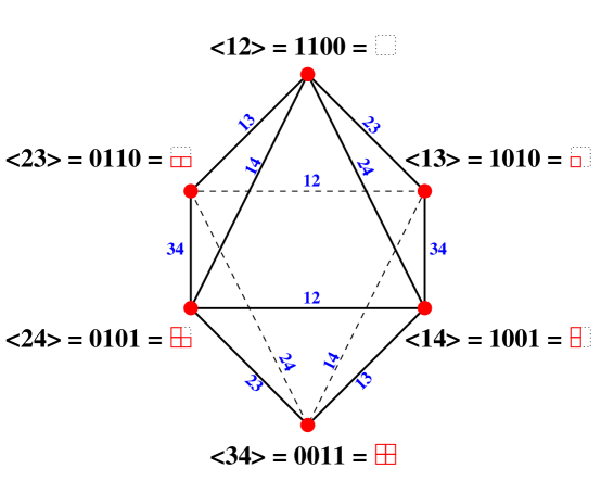
Figure 22: The Schubert cells of the Grassmannian (as well as vacua of 4d ${\mathcal{N}}=2$ SQCD) can be labeled by Young diagrams that fit into $r\times(N-r)$ rectangle, or, equivalently, by a string that contains $r$ ones and $N-r$ zeros, or, yet another way, by length-$r$ subsets $I\subset\{1,\ldots,N\}$. Shown here is the example with $r=2$ and $N=4$.

The quantum and equivariant deformations of the cohomology ring (82) can be combined into the $T$-equivariant quantum cohomology of $Gr(r,N)$ which has multiplication of the form (83), where the equivariant quantum Littlewood-Richardson coefficients $c_{\lambda,\mu}^{\nu,d}$ are homogeneous polynomials in the ring (99) of degree $|\lambda|+|\mu|-|\nu|-Nd$. The explicit form of these polynomials for $Gr(2,4)$ can be found in [68, sec. 8]. In particular, $c_{\lambda,\mu}^{\nu,d}$ is equal to the quantum Littlewood-Richardson coefficient when $|\lambda|+|\mu|=|\nu|+Nd$, while for $d=0$ it is equal to the ordinary equivariant Littlewood-Richardson coefficient $c_{\lambda,\mu}^{\nu}$. The remarkable fact about the equivariant quantum Littlewood-Richardson coefficients is that they are homogeneous polynomials in variables $m_{1}-m_{2}$, $\ldots$, $m_{N-1}-m_{N}$ with positive coefficients. Hence, they can be categorified!

Domain walls in 4d ${\mathcal{N}}=2$ SQCD

The geometry of Schubert varieties described here has a simple interpretation in terms of moduli spaces of domain walls in 4d ${\mathcal{N}}=2$ super-QCD with $U(r)$ gauge group and $N_{f}=N$ flavors in the fundamental representation of the gauge group, see e.g. [69, 70, 71]. Since this physical manifestation is somewhat tangential to the subject of the present paper we relegate it to Appendix B.

4 Categorification and the Landau-Ginzburg perspective

As we already explained in section 2.4, surface operators supported on knot and graph cobordisms provide a categorification of the corresponding knot/graph invariants, thus making the results of section 3 directly relevant. Moreover, the choice of the Riemann surface $C$ in section 3 determines the type of knot homology that one finds. Thus, a compact Riemann surface $C$ typically leads to a singly-graded homology theory (see [20] for concrete examples). In this paper, we are mostly interested in applications to doubly-graded knot homologies categorifying quantum group invariants; in the language of section 3, they correspond to a somewhat peculiar choice $C\cong{\mathbb{R}}^{2}_{\epsilon}$ (= “cigar” in the Taub-NUT space) that we already encountered in section 3.2 and will describe in more detail below.

In particular, we describe junctions of surface operators from the perspective of the 2d TQFT on $\Sigma$. We restrict the discussion to surface operators associated with antisymmetric tensor products of the fundamental representation of $\mathfrak{sl}_{N}$. Generalization of the discussion below to $\mathfrak{sl}_{N|M}$ and to symmetric representations of $\mathfrak{sl}_{N}$ should provide categorification of the super $q$-Howe duality [72] and symmetric $q$-Howe duality [73], respectively. We leave these generalizations to future work.

4.1 Physics perspectives on categorification

Soon after the advent of the first homological knot invariants [40, 74, 75] it was proposed [76, 20] that, in general, knot homology should admit a physical interpretation as a $Q$-cohomology of a suitable physical system,

$$\text{knot homology}\;=\;Q\text{-cohomology}\;\equiv\;{\mathcal{H}}_{\text{BPS}}$$ (100)

where $Q$ is a supercharge. Since then, many concrete realizations of this general scenario have been proposed for different knot homologies.

In most of the physics approaches to knot homologies, the starting point is one of the two closely related fivebrane systems:

$$\begin{array}[]{rcl}\lx@intercol\hfil~{}~{}\text{doubly-graded}{}\hfil\lx@intercol\\[2.84544pt] \hline\cr{\mbox{\rm space-time:}}&&~{}~{}{\mathbb{R}}_{t}\times T^{*}S^{3}\times TN_{4}\\ {\mbox{\rm$N$ M5-branes:}}&&~{}~{}{\mathbb{R}}_{t}\times~{}S^{3}~{}\times~{}{\mathbb{R}}^{2}_{\epsilon}\\ {\mbox{\rm$k$ M5${}^{\prime}$-branes:}}&&~{}~{}{\mathbb{R}}_{t}\times~{}L_{\Gamma}~{}\times~{}{\mathbb{R}}^{2}_{\epsilon}\end{array}\quad\xleftarrow[~{}\text{transition}]{~{}\text{phase}}\!\!\!\to\quad\begin{array}[]{rcl}\lx@intercol\hfil~{}~{}~{}\text{triply-graded}{}{}\hfil\lx@intercol\\[2.84544pt] \hline\cr&&{\mathbb{R}}_{t}\times CY_{3}\times TN_{4}\\ &&{\mathbb{R}}_{t}\times~{}L_{\Gamma}\times{\mathbb{R}}^{2}_{\epsilon}\end{array}$$ (101)

which is precisely a variant of (54), with $M_{3}=S^{3}$ and $C={\mathbb{R}}_{\epsilon}^{2}$. (Other variants, with $C=S^{2}$ and $C=T^{2}$, have been studied in [20].) Keeping track of the $U(1)\times U(1)$ quantum numbers associated with the rotation symmetry of $C={\mathbb{R}}^{2}_{\epsilon}$ and its normal bundle in the Taub-NUT space where it is naturally embedded, $TN_{4}\cong T^{*}C$, leads to two gradings, namely the $q$-grading and the homological $t$-grading.

Much like the familiar phases of water, the two fivebrane configurations in (101) are conjecturally related by a phase transition [77, 78] and describe the same physical system in different regimes of parameters, one of which has the fixed rank $N$ and hence is more suited for doubly-graded knot homologies, while the other has an additional, third grading on the space of refined BPS states (= $Q$-cohomology) and provides a physical realization of colored HOMFLY-PT homologies. Studying the two fivebrane systems (101) from different vantage points led to different physical perspectives on doubly-graded and triply-graded knot homologies:

• Enumerative invariants: Looking at the system (101) from the vantage point of the Calabi-Yau space $CY_{3}$ leads to the original physical description [76] in terms of enumerative invariants.

• Refined Chern-Simons: Looking from the vantage point of $M_{3}=S^{3}$ on the doubly-graded side of (101) leads to $\mathfrak{sl}_{N}$ double affine Hecke algebra (DAHA) and refined Chern-Simons theory [79, 80, 81, 82, 83].

• 5d gauge theory: Also on the doubly-graded side, analyzing the system (101) from the vantage point of the world-volume theory on $N$ M5-branes leads to a formulation of knot homology via counting solutions to the Haydys-Witten equations in five dimensions [84, 85].

• Landau-Ginzburg model is a two-dimensional theory that “lives” on $(\text{time})\times(\text{knot})$ or, to be more precise, on the cylinder ${\mathbb{R}}_{t}\times S^{1}_{\sigma}$, where $S^{1}_{\sigma}\subset S^{3}$ is the great circle and $K\to S^{1}_{\sigma}$ is a multiple cover [44, 45, 86, 87]. In this description of doubly-graded $\mathfrak{sl}_{N}$ homology, each braiding (crossing) in a two-dimensional projection of a link $K$ is represented by the corresponding line defect $\mathcal{D}_{i}$ in the two-dimensional Landau-Ginzburg model, as illustrated in Figure 23.

• 3d ${\mathcal{N}}=2$ theory labeled by the knot $K$ that “lives” on a $3$-dimensional part, ${\mathbb{R}}_{t}\times{\mathbb{R}}^{2}_{\epsilon}$, of the fivebrane world-volume provides yet another way to compute the $Q$-cohomology on either side of (101). This approach is a certain variant of the so-called “3d-3d correspondence” [88, 89].

• Vortex counting: Compactification of M-theory on the Calabi-Yau $3$-fold $CY_{3}$ is known to engineer 5d ${\mathcal{N}}=2$ gauge theory [90], in which fivebranes (101) produce a codimension-$2$ defect, a “surface operator”. Thus, from the vantage point of 5d gauge theory on ${\mathbb{R}}_{t}\times TN_{4}$ with a ramification (determined by the knot $K$) along ${\mathbb{R}}_{t}\times{\mathbb{R}}^{2}_{\epsilon}$, the problem of counting BPS states can be formulated in terms of K-theoretic instanton-vortex counting [91, 39] that involves Hilbert schemes of points, etc.

These physical perspectives stimulated development of many new structures in knot homologies, including the formulation of triply-graded homology categorifying the HOMFLY-PT polynomial [92], which came as a bit of surprise [93], led to many new differentials (canceling, universal, colored, exceptional), to new connections with knot contact homology [94], recursion relations with respect to color-dependence [95], etc.

The setup (101) has a natural extension to knot cobordisms (on both sides, although the two extensions are not obviously related by a phase transition), cf. (48):

$$\begin{array}[]{rcl}\lx@intercol\hfil~{}~{}\text{doubly-graded}{}\hfil\lx@intercol\\[2.84544pt] \hline\cr{\mbox{\rm space-time:}}&&~{}~{}\Lambda^{2}_{+}(M_{4})\times TN_{4}\\ {\mbox{\rm$N$ M5-branes:}}&&~{}~{}~{}M_{4}~{}\times~{}R_{\epsilon}^{2}\\ {\mbox{\rm M5${}^{\prime}$-branes:}}&&~{}~{}~{}L_{\Sigma}~{}\times~{}R_{\epsilon}^{2}\end{array}\quad\qquad\quad\begin{array}[]{rcl}\lx@intercol\hfil~{}~{}~{}\text{triply-graded}{}{}\hfil\lx@intercol\\[2.84544pt] \hline\cr{\mbox{\rm space-time:}}&&~{}~{}X_{G2}\times TN_{4}\\ {\mbox{\rm M5${}^{\prime}$-branes:}}&&~{}L_{\Sigma}\times R_{\epsilon}^{2}\end{array}$$ (102)

where the cobordism $\Sigma$ combines the “time” direction and the direction along the knot into a non-trivial 2-manifold, $X_{G2}$ is a 7-manifold with $G_{2}$ holonomy (= ${\mathbb{R}}_{t}\times CY_{3}$ in simple cases), and $L_{\Sigma}$ is a coassociative submanifold described in (49).

A variant of the transition [56] relates the doubly-graded side of (101) and (102) with surface operators produced from codimension-2 defects on the fivebrane world-volume to similar brane configurations with M2-branes (codimension-4 surface operators). For instance, a suitable analogue of (102) is

$${\mbox{\rm space-time:}}\qquad\Lambda^{2}_{+}(M_{4}) \times TN_{4}$$

$${\mbox{\rm$N$ M5-branes:}}\qquad~{}~{}~{}M_{4}~{}~{}~{} \times R_{\epsilon}^{2}$$ (103)

$${\mbox{\rm M2-branes:}}\qquad\Sigma\;\times\!\!\!\!\!\widetilde{~{}}~{}\;{\mathbb{R}}_{+} \times ~{}\{0\}$$

where the twisted product $\Sigma\;\times\!\!\!\!\!\widetilde{~{}}~{}\;{\mathbb{R}}_{+}$ is an associative submanifold in $\Lambda^{2}_{+}(M_{4})$. In the special case $M_{4}={\mathbb{R}}_{t}\times S^{3}$ and $\Sigma={\mathbb{R}}_{t}\times\Gamma$ we find $\Lambda^{2}_{+}(M_{4})={\mathbb{R}}_{t}\times T^{*}S^{3}$ and $\Sigma\;\times\!\!\!\!\widetilde{~{}}~{}\;{\mathbb{R}}_{+}\cong{\mathbb{R}}_{t}\times\Gamma\times{\mathbb{R}}_{+}$.

Of particular interest is the cobordism representing the connected sum with the unknot (31) which can fully characterize the 2d “effective theory” that lives on patches of a general foam $\Sigma$.

4.2 LG theory on “time $\times$ knot”

Our next goal is to describe the effective 2d theory that “lives” on the world-sheet $\Sigma$ of surface operators which appear in categorification of quantum group invariants.

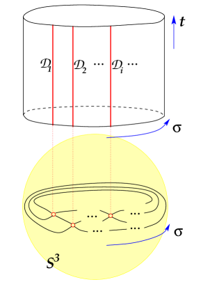
Figure 23: A knot or a link $K$ can be represented as a closure of a braid that runs along one of the directions in $M_{3}$ ($=S^{3}$ here). Then, crossings or braidings (denoted by “$\circ$”) of a surface operator in extra dimensions of $M_{3}$ “project” to interfaces in 2d Landau-Ginzburg model on ${\mathbb{R}}_{t}\times S^{1}_{\sigma}$.

The first clue comes from the early construction of knot homology groups [96, 92] based on matrix factorizations. Since matrix factorizations are known to describe boundary conditions and interfaces in 2d Landau-Ginzburg models [97, 98, 99, 23, 100, 101] it was proposed in [86, 87, 102] to interpret the matrix factorizations used by Khovanov and Rozansky as interfaces in 2d Landau-Ginzburg model on what we call $\Sigma$, i.e. on the product of the time direction ${\mathbb{R}}_{t}$ and the strands of a knot, or link, or tangle, as illustrated in Figure 23.

There are several ways to show this, including dualities that map intersecting branes in M-theory to intersecting D-branes which allow to address the question of what degrees of freedom live on $\Sigma$ via the standard tools of perturbative string theory. The upshot of this exercise is that for each strand in the braid or link $K$ colored by $R$ one finds a 2d theory whose chiral ring agrees with the homology of the unknot (32) colored by a representation $R$ of Lie algebra $\mathfrak{g}$.

Using this physical interpretation, not only can one reproduce the superpotential $W_{{\mathfrak{g}},R}(x)$ for $\mathfrak{g}=\mathfrak{sl}_{N}$ and $R=\Box$ used by Khovanov and Rozansky but also produce new Landau-Ginzburg potentials for more general representations. This includes all symmetric and anti-symmetric representations of $\mathfrak{g}=\mathfrak{sl}_{N}$, certain representations of exceptional Lie algebras and $\mathfrak{g}=\mathfrak{so}_{N}$ [86], which later were used in mathematical constructions of the corresponding knot homologies, see e.g. [103, 104, 28, 105].

In all of these constructions, the category (29) is a category of matrix factorizations $\text{MF}(W)$ of a polynomial

$$W=W_{R_{1}}+\ldots+W_{R_{n}}$$ (104)

that is a sum of potentials $W_{R_{i}}$, one for each marked point (or strand). Correspondingly, the category

$$\mathfrak{C}_{R_{1},\ldots,R_{n}}\;=\;\text{MF}(W)\;=\;\text{MF}(W_{R_{1}})\otimes\ldots\otimes\text{MF}(W_{R_{n}})$$ (105)

is a product of categories $\text{MF}(W_{R_{i}})$ associated to individual strands. As discussed in section 2.4, the Hochschild homology of the $\text{MF}(W_{R})$ is supposed to agree with the homology of the $R$-colored unknot,

$${\mathcal{A}}\;=\;HH^{*}\big{(}\text{MF}(W_{R})\big{)}\;=\;{\mathcal{H}}^{R}\big{(}{\,\raisebox{-2.27626pt}{\includegraphics[width=11.38092pt]{unknot}}\,}\big{)}$$ (106)

if the knot homology at hand extends to a functor (27), c.f. (30). The Hochschild homology can be computed as the the homology of the Koszul complex associated with the sequence of partial derivatives of $W_{R}$. It contains the Jacobi ring ${\mathcal{J}}(W_{R})$ and is in fact equal to it if and only if $W_{R}$ has only isolated singularities. Indeed, it is this case, which will be relevant for us. Hence, we get a non-trivial constraint on the superpotential $W_{R}$, namely that its Jacobi ring, which is also the chiral ring of the Landau-Ginzburg model associated to an $R$-colored point, has to agree with the respective knot homology. This identification has to hold on the level of algebras. (Recall that the knot homology carries an algebra structure containing information about knot cobordisms, c.f. the discussion around (33).)

Beyond this, also deformations of Khovanov-Rozansky homology groups categorifying quantum $\mathfrak{sl}_{N}$ invariants [33, 30, 35, 106, 32, 38] must be correctly incorporated in the structure of the category (29) associated to marked points. Indeed, this is not entirely unrelated from the algebra structure: differentials in spectral sequences that relate different variants of knot homology are often represented by generators of the algebra (32).

In the Landau-Ginzburg setup, such deformations should be realized by relevant deformations of the Landau-Ginzburg potential $W_{R}$, providing further consistency checks for the proposed Landau-Ginzburg description. Moreover, also the physically motivated generalizations of the original Khovanov-Rozansky construction to other representations mentioned above give further credence to the Landau-Ginzburg approach.

In addition, parallel developments in the study of surface operators led to a number of alternative descriptions of the chiral ring (106) which, in all cases of our interest, agrees with the chiral ring of the Landau-Ginzburg model with the superpotential $W_{R}$. Indeed, as we reviewed in section 3, the same brane configurations (102)–(103) that we use for categorification of quantum group invariants describe codimension-$2$ and codimension-$4$ defects in 6d theory on M5-branes. Thus, one can use the description of surface operators as coupled 2d-4d systems to describe the effective 2d theory on $\Sigma$.

Because the question about the chiral ring ${\mathcal{A}}$ of the 2d theory on $\Sigma$ is completely local (in a sense that it does not depend on the geometry away from $\Sigma$ as well as position along $\Sigma$), we can take $M_{4}={\mathbb{R}}^{4}$ and $\Sigma={\mathbb{R}}^{2}$. Then, the question basically reduces to the study of the chiral ring in 2d theory on the surface operator labeled by $R$ in 4d ${\mathcal{N}}=4$ gauge theory on $M_{4}$ that we already analyzed in section 3. In this paper, we are mainly interested in the case of the gauge group $G=SU(N)$ and its $k$-th anti-symmetric representation $R=\Lambda^{k}{\mathbb{C}}^{N}$. The corresponding surface operators have Levy type $\mathbb{L}=SU(U(k)\times U(N-k))$ and in the description as 2d-4d coupled systems à la (38), the 2d theory on $\Sigma$ is a ${\mathcal{N}}=(4,4)$ sigma-model with hyper-Kähler target space $T^{*}(G/\mathbb{L})=T^{*}Gr(k,N)$. Topological twist of the ambient theory on $M_{4}$ induces a topological twist of the 2d theory on $\Sigma$, which then becomes a 2d TQFT with the chiral ring

$${\mathcal{A}}\;=\;H^{*}(Gr(k,N))$$ (107)

given by the classical cohomology of the Grassmannian, in agreement with (34) and (81). A 2d TQFT with the same chiral ring can be obtained by a topological B-twist of the ${\mathcal{N}}=(2,2)$ Landau-Ginzburg model with $k$ chiral superfields $x_{1},\ldots,x_{k}$ of $U(1)_{R}$-charge $q={2\over N+1}$ and the superpotential

$$W_{0}(x_{1},\ldots,x_{k})=x_{1}^{N+1}+\ldots+x_{k}^{N+1}\,.$$ (108)

More precisely, a change of variables from the $x_{i}$ to the elementary symmetric polynomials $X_{i}=\sigma_{i}(x_{1},\ldots,x_{k})$ (see e.g. section 8.3 of [107]):

$$(x_{1},\ldots,x_{k})\longmapsto\left(X_{1}=\sigma_{1}(x_{1},\ldots,x_{k}),\ldots,X_{k}=\sigma_{k}(x_{1},\ldots,x_{k})\right)$$ (109)

gives rise to a new Landau-Ginzburg model denoted by $LG_{k}$. Its chiral superfields $X_{i}$ have $U(1)_{R}$-charge $q_{i}={2i\over N+1}$, and its superpotential $W=W(X_{1},\ldots,X_{k})$ is just $W_{0}$ expressed in terms of the $X_{i}$, i.e. $W(\sigma_{1}(x_{1},\ldots,x_{k}),\ldots,\sigma_{k}(x_{1},\ldots,x_{k}))=W_{0}(x_{1},\ldots,x_{k})$. It is still quasi-homogeneous. In the IR, $LG_{k}$ flows to a superconformal field theory of central charge

$$c={3k(N-k)\over N+1}\,,$$ (110)

which is believed to be the level-$1$ Kazama-Suzuki model associated to the Grassmannian $Gr(k,N)$. The chiral ring of $LG_{k}$ is the Jacobi ring of $W(X_{1},\ldots,X_{k})$ and indeed agrees with the classical cohomology ring $H^{*}(Gr(k,N))$ of the Grassmannian[66]. The chiral superfields $X_{i}$ correspond to the Chern classes $c_{i}$ of the tautological bundle over $Gr(k,N)$.

Note that the M-theory setup features two $U(1)$-symmetries induced by rotations in $TN_{4}$. One of them, namely the $q$-grading, descends to the $U(1)_{R}$-symmetry of the Landau-Ginzburg model. The other one will not play a role in our discussion.

4.3 Junctions and LG interfaces

Let us now turn to the Landau-Ginzburg description of junctions of surface operators. We are interested in junctions of surface operators which are created when the stack of $k$ M5^′-branes is split up into two stacks of $k_{1}$ and $k_{2}=k-k_{1}$ M5^′-branes, c.f. Figure 20 and Figure 24.

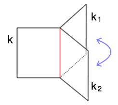
Figure 24: Junction between $LG_{k}$, $LG_{k_{1}}$ and $LG_{k_{2}=k-k_{1}}$. Upon folding it can be described by an interface $\mathcal{I}_{k}^{k_{1},k_{2}}$ between $LG_{k}$ and $LG_{k_{1}}\otimes LG_{k_{2}}$.

As we already discussed below (79), from the point of view of the Grassmannian sigma-model this splitting corresponds to the following boundary condition at the junction: the $k_{1}$- and $k_{2}$-dimensional subspaces defining the theory after the splitting are orthogonal at the point of splitting and span the $k=(k_{1}+k_{2})$-dimensional subspace defining the theory before the splitting. This condition can be described by means of the correspondence (44) between (products of) Grassmannians. It identifies the Chern classes $c^{(k)}_{1},\ldots,c^{(k)}_{k}$ of the tautological bundle over $Gr(k,N)$ with the symmetrizations

$$c^{(k)}_{i}=\sum_{j=0}^{i}c^{(k_{1})}_{j}c^{(k_{2})}_{i-j}$$ (111)

of the Chern classes $c^{(k_{i})}_{j}$ of the tautological bundles over $Gr(k_{i},N)$, see Appendix C.

This translates to a rather simple identification of chiral fields between the respective Landau-Ginzburg models: We regard the junction via the folding trick as an interface $\mathcal{I}_{k}^{k_{1},k_{2}}$ between Landau-Ginzburg models $LG_{k}$ on one side and $LG_{k_{1}}\otimes LG_{k_{2}}$ on the other. Both these theories can be realized by means of a change of variables from one and the same model, $LG_{1}^{\otimes k}$, the Landau-Ginzburg model with $k$ chiral superfields $x_{1},\ldots,x_{k}$ and superpotential (108). On the left side of the interface, in the model $LG_{k}$, the chiral superfields $X_{i}$ are obtained as the symmetrization of all the variables $x_{i}$, c.f. (109), and correspond to the Chern classes $c^{(k)}_{i}$ of $Gr(k,N)$. On the right side of the interface, the superfields of the model $LG_{k_{1}}\otimes LG_{k_{2}}$ are obtained by symmetrizing the first $k_{1}$ variables $(x_{1},\ldots,x_{k_{1}})$ and the last $k_{2}=k-k_{1}$ variables $(x_{k_{1}+1},\ldots,x_{k})$ separately:

$$(x_{1},\ldots,x_{k})\longmapsto(Y_{1},\ldots,Y_{k})=$$ (112)

$$\quad(\sigma_{1}(x_{1},\ldots,x_{k_{1}}),\ldots,\sigma_{k_{1}}(x_{1},\ldots,x_{k_{1}}),\sigma_{1}(x_{k_{1}+1},\ldots,x_{k}),\ldots,\sigma_{k_{2}}(x_{k_{1}+1},\ldots,x_{k}))\,.$$

The $Z_{i}=Y_{i}$, $i=1,\ldots,k_{1}$ and $Z^{\prime}_{j}=Y_{k_{1}+j}$, $j=1,\ldots,k_{2}$ are the superfields of the factor models $LG_{k_{1}}$ and $LG_{k_{2}}$, respectively, and can be identified with the Chern classes $c_{i}^{(k_{1})}$ and $c_{j}^{(k_{2})}$. In terms of these fields, the junction condition (111) reads

$$X_{i}=\sigma_{i}(x_{1},\ldots,x_{k})=f_{i}(Y_{1},\ldots,Y_{k})=\sum_{j=0}^{i}Z_{j}Z^{\prime}_{i-j}\,.$$ (113)

It trivially identifies the underlying models $LG_{1}^{\otimes k}$ on both sides of the interface, and identifies the more symmetric variables $X_{i}$ on its left with the respective symmetrization of the less symmetric variables $Y_{i}$ on its right:

$$X_{1} = \sigma_{1}(x_{1},\ldots,x_{k})=f_{1}(Y_{1},\ldots,Y_{k})=Y_{1}+Y_{k_{1}+1}\,,$$

$$X_{2} = \sigma_{2}(x_{1},\ldots,x_{k})=f_{2}(Y_{1},\ldots,Y_{k})=Y_{2}+Y_{k_{1}+2}+Y_{1}Y_{k_{1}+1}\,,$$

$$\ldots$$

This discussion immediately generalizes to more complicated configurations. The junction created by splitting up the stack of M5^′-branes into $r>2$ stacks of multiplicities $k_{1},\ldots,k_{r}$, respectively, on the level of the Grassmannian sigma-models is described by the correspondence via the partial flag manifold $Fl(k_{1},k_{1}+k_{2},\ldots,k_{1}+\ldots+k_{r}=k,N)=G/\mathbb{L}$ with the Levi subgroup $\mathbb{L}=S\big{(}\prod_{i}U(k_{i})\big{)}$, i.e. the space of flags

$${\mathbb{C}}^{k_{1}}\subset{\mathbb{C}}^{k_{1}+k_{2}}\subset\cdots\subset{\mathbb{C}}^{N}$$ (115)

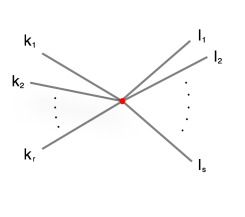
Figure 25: Interface $\mathcal{I}_{k_{1},\ldots,k_{r}}^{l_{1},\ldots,l_{s}}$ between $LG_{k_{1}}\otimes\ldots\otimes LG_{k_{r}}$ and $LG_{l_{1}}\otimes\ldots\otimes LG_{l_{s}}$.

As before, this translates to a simple condition at the interface $\mathcal{I}_{k}^{k_{1},\ldots,k_{r}}$ between the respective Landau-Ginzburg models, $LG_{k}$ on one side and $LG_{k_{1}}\otimes\ldots\otimes LG_{k_{r}}$ on the other. Again, both models can be obtained by different changes of variables from one and the same underlying model, $LG_{1}^{\otimes k}$, which is trivially identified by the interface. The superfields $X_{1},\ldots,X_{k}$ of $LG_{k}$ are the symmetrization of all the fields $x_{1},\ldots,x_{k}$, whereas the fields $Y_{1},\ldots,Y_{k}$ of $LG_{k_{1}}\otimes\ldots\otimes LG_{k_{r}}$ are obtained by separately symmetrizing the sets of variables $(x_{1},\ldots,x_{k_{1}})$, $(x_{k_{1}+1},\ldots,x_{k_{1}+k_{2}})$, $\ldots$, $(x_{k_{1}+\ldots+k_{r-1}+1},\ldots,x_{k})$. The interface then expresses the more symmetric polynomials $X_{i}$ in terms of the less symmetric ones $Y_{j}$:

$$X_{i}=\sigma_{i}(x_{1},\ldots,x_{k})=f_{i}^{\prime}(Y_{1},\ldots,Y_{k})\,.$$ (116)

From this it is also evident how to describe a junction at which $r$ stacks of M5^′-branes of multiplicities $k_{1},\ldots,k_{r}$ join and immediately split up into $s$ stacks or multiplicities $l_{1},\ldots,l_{s}$, c.f. Figure 25. (In this and the following figures we will suppress the time direction. The surface operators will be represented by lines, which will be labeled by the multiplicity of the respective stack of M5^′-branes. Surface operators also have an orientation, which, in case of ambiguity will be indicated by arrows. The junctions discussed here, which arise by splitting and joining of stacks of M5^′-branes have the property that the sum of labels of incoming lines equals the sum of labels of outgoing lines: M5^′-branes cannot end in junctions.) The junction of Figure 25 can be realized by an interface $\mathcal{I}_{k_{1},\ldots,k_{r}}^{l_{1},\ldots,l_{s}}$ between $LG_{k_{1}}\otimes\ldots\otimes LG_{k_{r}}$ on the left side and $LG_{l_{1}}\otimes\ldots\otimes LG_{l_{s}}$ on the right. Since $\sum_{i}k_{i}=k=\sum_{j}l_{j}$, the models on either side of the interface arise from one and the same model $LG_{1}^{\otimes k}$ by means of different symmetrizations of variables. On the left, the sets $(x_{1},\ldots,x_{k_{1}})$, $(x_{k_{1}+1},\ldots,x_{k_{1}+k_{2}})$, $\ldots$, $(x_{k_{1}+\ldots+k_{r-1}+1},\ldots,x_{k})$ are symmetrized separately giving rise to the chiral superfields $(X_{1},\ldots,X_{k})$, whereas on the right the superfields $(Y_{1},\ldots,Y_{k})$ are obtained by symmetrizing the $(x_{1},\ldots,x_{l_{1}})$, $(x_{l_{1}+1},\ldots,x_{l_{1}+l_{2}})$, $\ldots$, $(x_{l_{1}+\ldots+l_{s-1}+1},\ldots,x_{k})$. The interface now relates the fields on the two sides of the defect by expressing the symmetric polynomials $\sigma_{i}(x_{1},\ldots,x_{k})$ in terms of the partially symmetrized ones on either side:

$$f^{\prime}_{1}(X_{1},\ldots,X_{k})= \sigma_{1}(x_{1},\ldots,x_{k}) =f^{\prime\prime}_{1}(Y_{1},\ldots,Y_{k})$$

$$f^{\prime}_{2}(X_{1},\ldots,X_{k})= \sigma_{2}(x_{1},\ldots,x_{k}) =f^{\prime\prime}_{2}(Y_{1},\ldots,Y_{k})$$

$$\ldots \,,$$

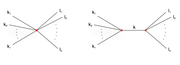
Figure 26: Junction described by $\mathcal{I}_{k_{1},\ldots,k_{r}}^{l_{1},\ldots,l_{s}}$ (left) factorizes as $\mathcal{I}_{k_{1},\ldots,r_{r}}^{k}*\mathcal{I}_{k}^{l_{1},\ldots,l_{s}}$ over $LG_{k}$ (right).

In particular, this condition is the composition of the identifications imposed by the interfaces $\mathcal{I}_{l_{1},\ldots,l_{s}}^{k}$ describing the splitting of one stack into $s$ stacks and the one imposed by the interface $\mathcal{I}_{k}^{k_{1},\ldots,k_{r}}$ describing the joining of the $r$ stacks into one stack. Thus, the respective interface can be obtained by fusion

$$\mathcal{I}_{k_{1},\ldots,k_{r}}^{l_{1},\ldots,l_{s}}=\mathcal{I}_{k_{1},\ldots,r_{r}}^{k}*\mathcal{I}_{k}^{l_{1},\ldots,l_{s}}\,$$ (118)

of these two interfaces over $LG_{k}$, c.f. Figure 26.

In fact, more generally, the interfaces $\mathcal{I}_{k_{1},\ldots,k_{r}}^{l_{1},\ldots,l_{s}}$ factorize into those interfaces describing trivalent junctions (where either two stacks of M5^′-branes join into one or one stack splits up into two stacks), see Figure 27.

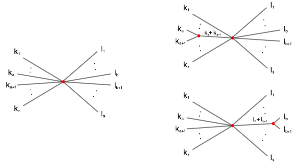
Figure 27: Junction (left) can be factorized into trivalent junctions (right).

4.4 Junctions and matrix factorizations

In the following, we will study the junctions of surface operators introduced in the last section in more detail using an elegant representation of interfaces between Landau-Ginzburg models in terms of matrix factorizations [23]. This representation in particular lends itself easily to the description of fusion. (Of course one could equivalently use the language of correspondences in Grassmannian sigma model to do the analysis.)

A matrix factorization over a polynomial ring $\mathcal{R}$ of a polynomial $W\in\mathcal{R}$ is a pair of square matrices $p_{0}$ and $p_{1}$ with entries in $\mathcal{R}$, which multiply to $W$ times the identity matrix:

$${\mathcal{P}}:\quad P_{1}\cong{\mathcal{R}}^{r}\overset{p_{1}}{\underset{p_{0}}{\mathrel{\begin{subarray}{c}\xrightarrow{\hskip 45.52458pt}\\[-2.58334pt] \xleftarrow{\hskip 45.52458pt}\end{subarray}}}}{\mathcal{R}}^{r}\cong P_{0}\,,\qquad p_{1}p_{0}=W{\rm id}_{P_{0}}\,,\quad p_{0}p_{1}=W{\rm id}_{P_{1}}\,.$$ (119)

A B-type supersymmetric interface connecting a Landau-Ginzburg model with chiral superfields $X_{1},\ldots,X_{k}$ and superpotential $W(X_{1},\ldots,X_{k})$ to one with superfields $Y_{1},\ldots,Y_{l}$ and superpotential $W^{\prime}(Y_{1},\ldots,Y_{l})$ is determined by a matrix factorization of the difference $W(X_{1},\ldots,X_{k})-W^{\prime}(Y_{1},\ldots,Y_{l})$ of superpotentials over the ring $\mathcal{R}={\mathbb{C}}[X_{1},\ldots,X_{k},Y_{1},\ldots,Y_{l}]$ of polynomials in the chiral superfields on both sides.

From this description it is easy to read off certain properties of the interface, such as the chiral ring of operators on the interface, which is given by the BRST-cohomology on ${\rm End}_{\mathcal{R}}(P_{0}\oplus P_{1})$, where the BRST-operator $Q$ acts on $\Phi\in{\rm End}_{\mathcal{R}}(P_{0}\oplus P_{1})$ by graded commutator

$$Q\Phi=p\,\Phi-\sigma\Phi\sigma\,p$$ (120)

with the operator

$$p=\left(\begin{array}[]{cc}0&p_{1}\\ p_{0}&0\end{array}\right)\,.$$ (121)

The ${\mathbb{Z}}_{2}$-grading (fermion number) is given by

$$\sigma=\left(\begin{array}[]{cc}{\rm id}_{P_{0}}&0\\ 0&-{\rm id}_{P_{1}}\end{array}\right)\,.$$ (122)

Correlation functions of chiral primary fields in the presence of such interfaces can be calculated by means of a residue formula [98].

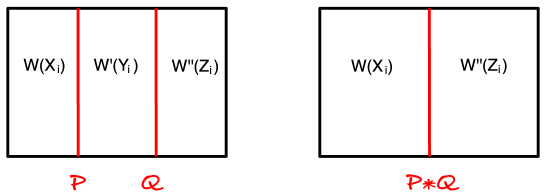
Figure 28: Fusion of interface $\mathcal{P}$ between LG models with superpotentials $W(X_{i})$ and $W^{\prime}(Y_{i})$, and $\mathcal{Q}$ between LG models with superpotentials $W^{\prime}(Y_{i})$ and $W^{\prime\prime}(Z_{i})$ (left) gives rise to interface $\mathcal{P}*\mathcal{Q}$ between LG models with superpotentials $W(X_{i})$ and $W^{\prime\prime}(Z_{i})$ (right).

Moreover, fusion of interfaces ${\mathcal{P}}$ and ${\mathcal{Q}}$ separating respectively a Landau-Ginzburg model with superpotential $W(X_{1},\ldots,X_{r})$ from one with superpotential $W^{\prime}(Y_{1},\ldots,Y_{s})$, and the model with superpotential $W^{\prime}(Y_{1},\ldots,Y_{s})$ from one with superpotential $W^{\prime\prime}(Z_{1},\ldots,Z_{t})$, c.f. Figure 28, has a very simple description in terms of matrix factorizations. The interfaces are described by two matrix factorizations

$${\mathcal{P}}:\;P_{1}\overset{p_{1}}{\underset{p_{0}}{\mathrel{\begin{subarray}{c}\xrightarrow{\hskip 45.52458pt}\\[-2.58334pt] \xleftarrow{\hskip 45.52458pt}\end{subarray}}}}P_{0}\quad{\rm and}\quad{\mathcal{Q}}:\;Q_{1}\overset{q_{1}}{\underset{q_{0}}{\mathrel{\begin{subarray}{c}\xrightarrow{\hskip 45.52458pt}\\[-2.58334pt] \xleftarrow{\hskip 45.52458pt}\end{subarray}}}}Q_{0}$$ (123)

of $W(X_{1},\ldots,X_{r})-W^{\prime}(Y_{1},\ldots,Y_{s})$ and $W^{\prime}(Y_{1},\ldots,Y_{s})-W^{\prime\prime}(Z_{1},\ldots,Z_{t})$, respectively. The fused interface ${\mathcal{P}}*{\mathcal{Q}}$ separates the Landau-Ginzburg models with superpotential $W(X_{1},\ldots,X_{r})$ from the one with superpotential $W^{\prime\prime}(Z_{1},\ldots,Z_{t})$. It is described by the tensor product matrix factorization

$$\left({\mathcal{P}}\otimes{\mathcal{Q}}\right)_{1}:=\left(\begin{array}[]{c}P_{1}\otimes Q_{0}\\ \oplus\\ P_{0}\otimes Q_{1}\end{array}\right)\overset{\left(\begin{array}[]{cc}p_{1}\otimes{\rm id}_{Q_{0}}&-{\rm id}_{P_{0}}\otimes q_{1}\\ {\rm id}_{P_{1}}\otimes q_{0}&p_{0}\otimes{\rm id}_{Q_{1}}\end{array}\right)}{\underset{\left(\begin{array}[]{cc}p_{0}\otimes{\rm id}_{Q_{0}}&{\rm id}_{P_{1}}\otimes q_{1}\\ -{\rm id}_{P_{0}}\otimes q_{0}&p_{1}\otimes{\rm id}_{Q_{1}}\end{array}\right)}{\mathrel{\begin{subarray}{c}\xrightarrow{\hskip 113.81102pt}\\[-2.58334pt] \xleftarrow{\hskip 113.81102pt}\end{subarray}}}}\left(\begin{array}[]{c}P_{0}\otimes Q_{0}\\ \oplus\\ P_{1}\otimes Q_{1}\end{array}\right)=:\left({\mathcal{P}}\otimes{\mathcal{Q}}\right)_{0}\,.$$ (124)

This is a matrix factorization of the sum

$$\left(W(X_{1},\ldots,X_{r})-W^{\prime}(Y_{1},\ldots,Y_{s})\right)+\left(W^{\prime}(Y_{1},\ldots,Y_{s})-W^{\prime\prime}(Z_{1},\ldots,Z_{t})\right)$$ (125)

$$\qquad\qquad\qquad\qquad\qquad\qquad\qquad\qquad\qquad\qquad=W(X_{1},\ldots,X_{r})-W^{\prime\prime}(Z_{1},\ldots,Z_{t})\,,$$

as it should be. It still involves the fields $Y_{i}$ of the Landau-Ginzburg model squeezed in between the interfaces, which are promoted to new degrees of freedom on the interface. Therefore, a priori it is a matrix factorization of infinite rank over ${\mathbb{C}}[X_{1},\ldots,X_{r},Z_{1},\ldots,Z_{t}]$. However, it can be shown that by splitting off “trivial” matrix factorizations these matrix factorizations always reduce to finite rank. See [23, 109, 87] for a more detailed discussion of fusion in this context.

The Landau-Ginzburg models we are interested in here exhibit a $U(1)_{R}$-symmetry, and the interfaces also preserve this symmetry. This means that the modules $P_{0}$ and $P_{1}$ carry representations $\rho_{0}$ and $\rho_{1}$ of $U(1)_{R}$, respectively, which are compatible with the $\mathcal{R}$-module structure, such that $p_{0}$ and $p_{1}$ are homogeneous of charge $1$. The respective matrix factorization is called “graded”. For ease of notation we will rescale the $U(1)_{R}$-charges by the degree $N+1$ of the potential. In these units the superpotential has charge $2N+2$, the maps $p_{i}$ have charge $N+1$, and the fields $X_{i}$ defined in (109) have charge $2i$. All charges appearing will be integral.

Now, the interface $\mathcal{I}_{k}^{k_{1},k_{2}}$ associated to the trivalent junction in Figure 24 separates the Landau-Ginzburg model $LG_{k}$ with superpotential $W(X_{1},\ldots,X_{k})$ (the superpotential of (108) written in the symmetrized fields (109)), from the Landau-Ginzburg model $LG_{k_{1}}\otimes LG_{k_{2}}$, which has superpotential $W(f_{1},\ldots,f_{k})$ (the same superpotential, but written in the only partially symmetrized fields (112)). Here $f_{i}=f_{i}(Y_{1},\ldots,Y_{k})$ is the map from (4.3) symmetrizing the partially symmetrized $Y_{i}$. The matrix factorization of $W(X_{1},\ldots,X_{k})-W(f_{1},\ldots,f_{k})$ which imposes the identification (4.3) is now easy to construct. It is given by a Koszul type matrix factorization, c.f. [23].

One can find homogeneous polynomials $U_{i}(X_{1},\ldots,X_{k},Y_{1},\ldots,Y_{k})$, $i=1,\ldots,k$, such that

$$W(X_{1},\ldots,X_{k})-W(f_{1},\ldots,f_{k})=\sum_{i=1}^{k}(X_{i}-f_{i}(Y_{1},\ldots,Y_{k}))\,U_{i}(X_{1},\ldots,X_{k},Y_{1},\ldots,Y_{k})\,.$$ (126)

One particular choice of such polynomials is given by

$$U_{i}={1\over X_{i}-f_{i}}\left(W(f_{1},\ldots,f_{i-1},X_{i},\ldots,X_{k})-W(f_{1},\ldots,f_{i},X_{i+1},\ldots,X_{k})\right)\,.$$ (127)

The matrix factorization describing the interface is then given by the tensor product

$$\mathcal{I}_{k}^{k_{1},k_{2}}=\left(\bigotimes_{i=1}^{k}{\mathcal{P}}^{i}\right)\{-k_{1}k_{2}\}$$ (128)

of the rank-$1$ matrix factorizations

$${\mathcal{P}}^{i}:\quad P^{i}_{1}\cong{\mathcal{R}}\{2i-N-1\}\overset{p^{i}_{1}=(X_{i}-f_{i})}{\underset{p^{i}_{0}=U_{i}}{\mathrel{\begin{subarray}{c}\xrightarrow{\hskip 45.52458pt}\\[-2.58334pt] \xleftarrow{\hskip 45.52458pt}\end{subarray}}}}{\mathcal{R}}\{0\}\cong P^{i}_{0}$$ (129)

over ${\mathcal{R}}={\mathbb{C}}[X_{1},\ldots,X_{k},Y_{1},\ldots,Y_{k}]$. Since, under the tensor product of matrix factorizations, the factorized polynomials behave additively, (128) is indeed a matrix factorization of (126) and has rank $r=2^{k-1}$. Here, with the notation ${\mathcal{R}}\{a\}$ we specify the $U(1)_{R}$-representations on ${\mathcal{R}}$ by indicating the charge $a$ of $1\in{\mathcal{R}}$; and a matrix factorization ${\mathcal{Q}}\{a\}$, as in (128), denotes the matrix factorization ${\mathcal{Q}}$ where all $U(1)_{R}$-charges are shifted by $a$.

This construction immediately generalizes to the more general junctions $\mathcal{I}_{k_{1},\ldots,k_{r}}^{l_{1},\ldots,l_{s}}$ of Figure 25. The respective interface separates the Landau-Ginzburg model $LG_{k_{1}}\otimes\ldots\otimes LG_{k_{r}}$ on the left from $LG_{l_{1}}\otimes\ldots\otimes LG_{l_{s}}$ on the right. Both models are obtained from the Landau-Ginzburg model of (108) by means of different symmetrizations of the variables $x_{1},\ldots,x_{k}$. On the left, the sets of variables $(x_{1},\ldots,x_{k_{1}})$, $(x_{k_{1}+1},\ldots,x_{k_{1}+k_{2}})$, $\ldots$, $(x_{k_{1}+\ldots+k_{r-1}+1},\ldots,x_{k})$ are symmetrized separately, giving rise to the superfields $(X_{1},\ldots,X_{k})$, whereas on the right the superfields $(Y_{1},\ldots,Y_{k})$ are obtained by symmetrizing the sets of variables $(x_{1},\ldots,x_{l_{1}})$, $(x_{l_{1}+1},\ldots,x_{l_{1}+l_{2}})$, $\ldots$, $(x_{l_{1}+\ldots+l_{s-1}+1},\ldots,x_{k})$. The superpotentials on the two sides are just given by (108), expressed in terms of the respective superfields on the two sides. On the left it is $W(f^{\prime}_{1},\ldots,f^{\prime}_{k})$, and on the right $W(f^{\prime\prime}_{1},\ldots,f^{\prime\prime}_{k})$, where $f^{\prime}_{i}$ and $f^{\prime\prime}_{i}$ are the maps (4.3) symmetrizing the partially symmetric $(X_{1},\ldots,X_{k})$ and $(Y_{1},\ldots,Y_{k})$, respectively.

As for the trivalent case, the junction condition (4.3) can now be implemented by a Koszul matrix factorization. The polynomials

$$U_{i}={1\over f^{\prime}_{i}-f^{\prime\prime}_{i}}\left(W(f^{\prime\prime}_{1},\ldots,f^{\prime\prime}_{i-1},f^{\prime}_{i},\ldots,f^{\prime}_{k})-W(f^{\prime\prime}_{1},\ldots,f^{\prime\prime}_{i},f^{\prime}_{i+1},\ldots,f^{\prime}_{k})\right)\,,$$ (130)

satisfy

$$W(f^{\prime}_{1},\ldots,f^{\prime}_{k})-W(f^{\prime\prime}_{1},\ldots,f^{\prime\prime}_{k})=\sum_{i=1}^{k}(f^{\prime}_{i}-f^{\prime\prime}_{i})\,U_{i}\,,$$ (131)

and the tensor product

$$\mathcal{I}_{k_{1},\ldots,k_{r}}^{l_{1},\ldots,l_{s}}=\left(\bigotimes_{i=1}^{k}{\mathcal{P}}^{i}\right){\scriptstyle\left\{{-\sum_{1\leq a<b\leq k}l_{a}l_{b}}\right\}}$$ (132)

of the rank-one matrix factorizations

$${\mathcal{P}}^{i}:\quad P^{i}_{1}\cong{\mathcal{R}}\{2i-N-1\}\overset{p^{i}_{1}=(f^{\prime}_{i}-f^{\prime\prime}_{i})}{\underset{p^{i}_{0}=U_{i}}{\mathrel{\begin{subarray}{c}\xrightarrow{\hskip 45.52458pt}\\[-2.58334pt] \xleftarrow{\hskip 45.52458pt}\end{subarray}}}}{\mathcal{R}}\{0\}\cong P^{i}_{0}$$ (133)

implements the identification (4.3) across the interface.

4.5 Junctions and categorification of quantum groups

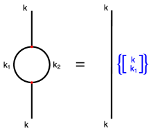
Figure 29: Fusion of $\mathcal{I}^{k}_{k_{1},k_{2}}$ and $\mathcal{I}^{k_{1},k_{2}}_{k}$ in $LG_{k_{1}}\otimes LG_{k_{2}}$ produces copies of the identity defect in $LG_{k}$.

The interfaces described in the last section satisfy many interesting properties. For instance, from the construction it is evident, that they factorize through a surface operator $LG_{k}$, i.e.

$$\mathcal{I}_{k_{1},\ldots,k_{r}}^{l_{1},\ldots,l_{s}}=\mathcal{I}^{l_{1},\ldots,l_{s}}_{k}*\mathcal{I}_{k_{1},\ldots,k_{r}}^{k}\,,$$ (134)

c.f. Figure 26, and that more generally, they factorize into interfaces corresponding to trivalent junctions, as displayed in Figure 27.

Moreover, fusing the interfaces $\mathcal{I}^{k}_{k_{1},k_{2}}$ and $\mathcal{I}^{k_{1},k_{2}}_{k}$ ($k=k_{1}+k_{2}$) in $LG_{k_{1}}\otimes LG_{k_{2}}$ produces a number of copies of the identity defect ${\rm Id}_{k}=\mathcal{I}_{k}^{k}$ in $LG_{k}$:

$$\mathcal{I}^{k}_{k_{1},k_{2}}*\mathcal{I}^{k_{1},k_{2}}_{k}={\rm Id}_{k}\left\{k\brack k_{1}\right\}\,,$$ (135)

see Figure 29. Here, we use the notation ${\cal P}\{q^{a_{1}}+\ldots+q^{a_{r}}\}:={\cal P}\{a_{1}\}\oplus\ldots\oplus{\cal P}\{a_{r}\}$ for a matrix factorization ${\cal P}$, and, as before, ${k\brack k_{1}}={[k]!\over[k_{1}]![k-k_{1}]!}$ denotes the quantum binomial coefficient with $[k]!=[k][k-1]\cdots[1]$, $[k]={q^{k}-q^{-k}\over q-q^{-1}}=q^{k-1}+q^{k-3}+\ldots+q^{-k+1}$. A simple proof of this relation can be found in Appendix D.1.

Let

$${\mathcal{E}}_{k_{1},k_{2}} := \left({\rm Id}_{k_{1}-1}\otimes\mathcal{I}_{1,k_{2}}^{k_{2}+1}\right)*\left(\mathcal{I}_{k_{1}}^{k_{1}-1,1}\otimes{\rm Id}_{k_{2}}\right)$$ (136)

$${\mathcal{F}}_{k_{1},k_{2}} := \left(\mathcal{I}_{k_{1},1}^{k_{1}+1}\otimes{\rm Id}_{k_{2}-1}\right)*\left({\rm Id}_{k_{1}}\otimes\mathcal{I}_{k_{2}}^{1,k_{2}-1}\right)\,,$$

be the combination of interfaces represented in Figure 30. Then, it is not difficult to see (c.f. Appendix D.2) that

$${\mathcal{E}}_{k_{1}+1,k_{2}-1}*{\mathcal{F}}_{k_{1},k_{2}}\cong{\mathcal{F}}_{k_{1}-1,k_{2}+1}*{\mathcal{E}}_{k_{1},k_{2}}\oplus{\rm Id}_{k_{1},k_{2}}\{\left[k_{2}-k_{1}\right]\}$$ (137)

for $k_{1}\leq k_{1}$ and

$${\mathcal{F}}_{k_{1}-1,k_{2}+1}*{\mathcal{E}}_{k_{1},k_{2}}\cong{\mathcal{E}}_{k_{1}+1,k_{2}-1}*{\mathcal{F}}_{k_{1},k_{2}}\oplus{\rm Id}_{k_{1},k_{2}}\{\left[k_{1}-k_{2}\right]\}$$ (138)

for $k_{1}\geq k_{2}$.

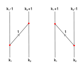
Figure 30: Configurations of surface operators categorifying the quantum group generators: ${\mathcal{E}}_{k_{1},k_{2}}$ (left) and ${\mathcal{F}}_{k_{1},k_{2}}$ (right).

Here ${\rm Id}_{k_{1},k_{2}}={\rm Id}_{k_{1}}\otimes{\rm Id}_{k_{2}}$ denotes the identity defect in the tensor product $LG_{k_{1}}\otimes LG_{k_{2}}$. But this is nothing but a categorification of the relation $[E,F]1_{n}=[n]1_{n}$ of the quantum group $\dot{\mathbf{U}}_{q}(\mathfrak{sl}_{2})$, c.f. (22). Here, the difference $n=k_{2}-k_{1}$ plays the role of a $\mathfrak{sl}_{2}$ weight.

In fact, the matrix factorizations $\mathcal{I}_{k_{1},\ldots,k_{r}}^{l_{1},\ldots,l_{s}}$ have already appeared in the construction of $\mathfrak{sl}_{N}$-link homology in the math literature [28]. There it was shown that they satisfy relations categorifying the MOY relations depicted in Figure 10. This means in particular, that the junctions of surface operators defined in section 4.3 provide a categorification of the $\dot{\mathbf{U}}_{q}(\mathfrak{sl}_{m})$ representation obtained by ladders of Wilson lines in Chern-Simons theory, c.f. section 2. This 2-representation was analysed from a mathematical point of view in [111]. Building blocks are configurations of $m$ parallel stacks of M5^′-branes, on which the quantum group generators ${\mathcal{E}}_{i}$ act by peeling off one M5^′-brane from the $i$-th stack and migrating it to the $(i+1)$-st stack, whereas the ${\mathcal{F}}_{i}$ are realized by peeling off one M5^′-brane from the $(i+1)$-st and moving it to the $i$-th stack.

The 2-category structure is given as follows: Objects are $m$-tuples $(k_{1},\ldots,k_{m})$, $0\leq k_{i}\leq N$, corresponding to $m$ parallel stacks of M5^′-branes of multiplicities $k_{i}$. From a 2d perspective they are realized by tensor products $LG_{k_{1}}\otimes\ldots\otimes LG_{k_{m}}$ of the Landau-Ginzburg theories on the respective world-volumes. 1-Morphisms correspond to configurations joining such stacks. In 2d they are interfaces between the respective Landau-Ginzburg models. The $2$-morphisms correspond to interface changing fields.

5 What’s next?

We conclude with a list of questions and possible generalizations, some of which have already been mentioned in the text:

• Even though the current work shows how the BPS junctions of surface operators realize the generators and elementary relations of the 2-category $\dot{\mathcal{U}}$, it still remains unproven whether these junctions reproduce the entire set of KLR algebra relations, or equivalently, the foam relations given in [18].

• It would be interesting to verify the existence of BPS junctions of surface operators by alternative methods (in particular, by constructing explicit solutions to the field equations) and extend the classification presented here to more general 4d theories and more general surface operators.

• For example, it would be interesting to construct holographic duals of surface operator junctions proposed here.

• Also it would be interesting to investigate, whether the categories of junctions of surface operators can be reconstructed out of the representation varieties appearing in the discussion of the charge conservation condition at junctions in section 3.5.

• Mathematically, other types of junctions (for other types of surface operators and LG models) also lead to diagrammatic algebras and may be worth exploring.

• As a generalization in a different direction, one may keep the same types of surface operators and LG interfaces, but consider changing space-time geometry, in particular, the geometry of the fivebrane world-volume. Indeed, in most of our discussion we assumed $M_{3}={\mathbb{R}}^{3}$, and one immediate generalization would be to consider $M_{3}=S^{1}\times{\mathbb{R}}^{2}$ which would result in planar diagrammatics on a cylinder. More generally, one might consider junctions of surface operators in $M_{4}=\widetilde{\Sigma}\times{\mathbb{R}}^{2}$ which, via the arguments of this paper, would lead to LG models and planar diagrammatics on a Riemann surface $\widetilde{\Sigma}$.

• The analysis of section 3 suggests to carry out the analogue of [63, 64] for the complexified gauge group $G_{{\mathbb{C}}}$ and to compare Poincaré polynomials of the resulting moduli spaces ${\mathcal{M}}(G_{{\mathbb{C}}},\Gamma)$ to MOY polynomials of the planar graphs $\Gamma$.

• In section 4 we already mentioned two important generalizations to supergroups and symmetric representations that should categorify the super $q$-Howe duality [72] and symmetric $q$-Howe duality [73], respectively.

• It would be interesting to work out a precise dictionary between “fake bubbles” of the diagrammatic approach [14] and relevant deformations of the Landau-Ginzburg potential [86], both of which are related to differentials on Khovanov-Rozansky homology.

We plan to tackle some of these questions in the future work.

Appendix A Wilson lines and categories $N$Web

In this section, we derive the remaining relations of Figure 10. Before proceeding to the derivations, however, it is necessary to resolve an ambiguity in our normalization. Let us denote the invariant tensors at the junctions of Figure 7 as $\epsilon_{k_{1},k_{2}}$ and $\widetilde{\epsilon}_{k_{1},k_{2}}$, respectively. Since the RHS of Figure 7 only determines the normalization of their product, it remains the same if one invariant tensor is multiplied by a complex number and the other by the inverse. Thus, there is an ambiguity in the “relative” normalization among the invariant tensors from different types of junctions. Such ambiguity would not be observed if $\epsilon$’s and $\widetilde{\epsilon}$’s always appear in pairs, but they do not in Figure 10(a), 10(d) and 10(f).

Figure 31: (a) Definition of $\eta_{i}$ and the closed Wilson lines which determine the value of $\eta_{i}^{2}$. (b) Renormalization of junctions which involve the Wilson lines in $\square$.

We claim that the junctions can be normalized so as to satisfy the relations of Figure 10. Let us first normalize those which involve Wilson lines in the defining representations. The open Wilson lines of Figure 31(a) are proportional to each other, since the associated Hilbert space is 1-dimensional. Renormalize the invariant tensors $\epsilon_{i,1}$ and $\epsilon_{1,i}$ via multiplication by $\eta_{i}$ (c.f. Figure 31(b)), and renormalize $\widetilde{\epsilon}_{i,1}$ and $\widetilde{\epsilon}_{1,i}$ accordingly via multiplication by $1/\eta_{i}$. This proves Figure 10(a) for $j=k=1$.

Inductively renormalize the junctions of higher rank representations. Consider Wilson lines of Figure 10(a) with $j=1$, and assume WLOG that $i\geq k$. Since the associated Hilbert space is 1-dimensional, the Wilson lines on each side are proportional to each other. Renormalizing $\epsilon_{i,k+1}$ by absorbing the proportionality constant, we have turned the relation into an identity and determined the relative normalization between $\epsilon_{i,k+1}$ and $\epsilon_{i+1,k}$. Proceed recursively until we reach $\epsilon_{i+k,1}$, whose normalization is fixed by Figure 31(b). Applying this procedure for all $i+k$, the relative normalizations among the invariant tensors can be determined such that Figure 10(a) holds for $j=1$. Finally, induction on $j$ shows that Figure 10(a) holds for any $i,j$ and $k$ (c.f. Figure 32.)

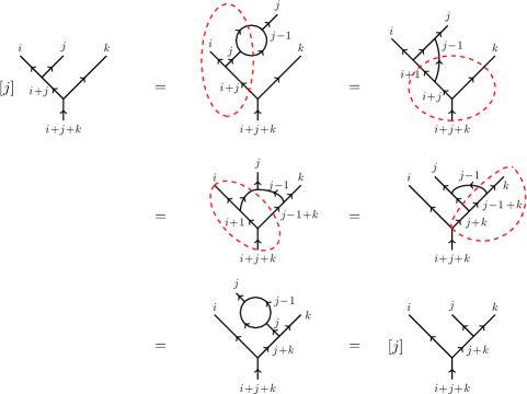
Figure 32: Induction on $j$. Apply the base case $j=1$ and the induction hypothesis for $j-1$ in the red dashed cirlces.

Now that we have fixed the normalization of junctions, let us proceed to derive the remaining relations. Figure 10(b) is rather straightforward, once we close the open ends by connecting them.

The three vectors of Figure 10(c) satisfy a linear relation, as the associated Hilbert space is 2-dimensional. Close the open ends in two inequivalent ways (c.f. Figure 12.) The resulting closed Wilson lines have computable expectation values via the direct sum formula, Figure 10(a) and Figure 10(b).

Figure 10(d) follows from Figures 10(a), (b) and (e). First, apply Figure 10(a) and 10(b) to replace the right-moving Wilson line labeled by $\wedge^{n}\square$ (the left-moving Wilson line labeled by $\wedge^{l+n-1}\square$) by $n$ right-moving Wilson lines labeled by $\square$ ($l\!+\!n\!-\!1$ left-moving Wilson lines labeled by $\square$). Recursively apply Figure 10(e) until the resulting Wilson lines are those of the RHS, and the coefficients follow.

Figure 10(f) also follows from Figures 10(a), (b) and (e). First, apply Figure 10(a) on LHS with $(i,j,k)=(m\!-\!2,1,1)$. Use Figure 10(a) and (b) to replace the upper Wilson line labeled by $\wedge^{j}\square$ by $j$ Wilson lines labeled by $\square$. Then, recursively apply Figure 10(e) until the resulting Wilson lines differ from those of the RHS only by a single right-moving Wilson line labeled by $\wedge^{2}\square$. Use Figure 10(a) and (b) to replace the latter by two Wilson lines labeled by $\square$, and the coefficients follow. This concludes our proof of Figure 10.

Appendix B Domain walls, junctions and Grassmannians

For $N>r$, and for generic values of mass parameters $m_{i}$, 4d ${\mathcal{N}}=2$ SQCD theory has massive isolated vacua (with $i_{n}<i_{n+1}$):

$$\phi\;=\;\text{diag}(m_{i_{1}},m_{i_{2}},\ldots,m_{i_{r}})$$ (139)

in which the gauge group $U(r)$ is completely broken and $SU(N_{f})\to U(1)^{N_{f}-1}$. When all masses are real — as e.g. in 5d lift of this theory — one can also assume $m_{i}<m_{i+1}$. Clearly, the set of such vacua is in one-to-one correspondence with Schubert cells ${\mathcal{S}}_{I}$ in $Gr(r,N)$ or, equivalently, vertices of the moment graph associated to the $T=U(1)^{N}$ action on $Gr(r,N)$ discussed around (97).

Note, that the mass parameters $m_{i}$ can be identified with the equivariant parameters for the torus action. For instance, $U(2)$ theory with $N_{f}=4$ has six vacua (92), also shown in Figure 22.

While vacua of 4d ${\mathcal{N}}=2$ SQCD correspond to vertices of the moment graph, elementary (not composite) domain walls that interpolate between vacua labeled by $I$ and $J$ correspond to edges of the moment graph connecting vertices $I$ and $J$. Two vertices $I\neq J$ are joined by an edge if and only if

$$|I\cup J|\;=\;r-1$$ (140)

in which case this edge is labeled by $m_{i}-m_{j}$, where $i$ and $j$ are the two elements in the symmetric difference of $I$ and $J$. For instance, $U(2)$ theory with $N_{f}=4$ has 12 elementary walls that correspond to edges of the octahedron in Figure 22. In general, each elementary wall carries $U(1)\subset U(r)$ symmetry left unbroken by $r-1$ components of the Higgs field which remain non-zero in the core of the wall in the weak coupling limit. For this reason, such elementary walls are called abelian [112]. For special values of mass parameters, one finds walls that support non-abelian symmetries [113, 71].

The BPS condition relates the domain wall tension $T$ and its orientation, say, in the $(x^{1},x^{2})$ plane to the absolute value and phase of $m_{i}-m_{j}$, respectively:

$$m_{i}-m_{j}=Te^{i\theta}$$ (141)

where $\theta$ is the angle in the $(x^{1},x^{2})$ plane. In particular, if all mass parameters $m_{i}$ are real, the BPS condition means that walls must be parallel in four-dimensional space-time and their ordering in $x^{2}$ direction precisely follows the closure ordering of Schubert cells (91). When mass parameters are complex, on the other hand, in general one finds a web (or network) of walls at angles determined by (141), see e.g. [114] for a nice “adiabatic” argument (for small values of $\text{Im}(m_{i})$).

Webs or networks of domain walls involve junctions, which can be either abelian or non-abelian, depending on the unbroken gauge symmetry in the core of the junction at weak coupling [112]. Specifically, a trivalent junction of walls separating vacua labeled by Schubert symbols $I_{1}=\langle a\,\underline{\cdots}\rangle$, $I_{2}=\langle b\,\underline{\cdots}\rangle$, and $I_{3}=\langle c\,\underline{\cdots}\rangle$ has vanishing components of the Higgs field $\phi_{a}$, $\phi_{b}$, and $\phi_{c}$ in the core of the junction and, therefore, carries $U(1)$ gauge symmetry left unbroken by the remaining $r-1$ non-zero components of the Higgs field. On the other hand, a junction of walls between vacua labeled by $I_{1}=\langle ab\,\underline{\cdots}\rangle$, $I_{2}=\langle bc\,\underline{\cdots}\rangle$, and $I_{3}=\langle ac\,\underline{\cdots}\rangle$ has only $r-2$ non-zero components of the Higgs field at the core and, therefore, carries $U(2)$ unbroken symmetry. This discussion easily generalizes to other types of walls and junctions.

Appendix C LG Interfaces and the cohomology of Grassmannians

The cohomology of the Grassmannian $Gr(k,N)$ can be described as the polynomial ring in the Chern classes $c_{1}^{(k)},\ldots,c_{k}^{(k)}$ of the tautological bundle and the Chern classes $\overline{c}^{(k)}_{1},\ldots,\overline{c}^{(k)}_{N-k}$ of the complementary bundle modulo the ideal $I_{k,N}$ generated by the relations

$$(1+tc^{(k)}_{1}+\ldots+t^{k}c^{(k)}_{k})(1+t\overline{c}^{(k)}_{1}+\ldots+t^{N-k}\overline{c}^{(k)}_{N-k})=1\,.$$ (142)

Similarly, the cohomology of the partial flag variety $Fl(k_{1},k=k_{1}+k_{2},N)$ can be realized as polynomial ring in $c_{1},\ldots,c_{k_{1}},c^{\prime}_{1},\ldots,c^{\prime}_{k_{2}},\overline{c}_{1},\ldots,\overline{c}_{N-k}$ modulo the ideal $I_{k_{1},k,N}$ generated by the relations

$$(1+tc_{1}+\ldots+t^{k_{1}}c_{k_{1}})(1+tc^{\prime}_{1}+\ldots+t^{k_{2}}c^{\prime}_{k_{2}})(1+t\overline{c}+\ldots+t^{N-k}\overline{c}_{N-k})=1\,.$$ (143)

Now (44) maps

$$H^{*}(Gr(k_{1},N)\times Gr(k_{2},N)) \longrightarrow H^{*}(Fl(k_{1},k,N))$$ (144)

$$c^{(k_{1})}_{i} \longmapsto c_{i}$$

$$\overline{c}^{(k_{1})}_{i} \longmapsto \sum_{j=0}^{i}c^{\prime}_{j}\overline{c}_{i-j}$$

$$c^{(k_{2})}_{i} \longmapsto c^{\prime}_{i}$$

$$\overline{c}^{(k_{2})}_{i} \longmapsto \sum_{j=0}^{i}c_{j}\overline{c}_{i-j}$$

and

$$H^{*}(Gr(k,N)) \longrightarrow H^{*}(Fl(k_{1},k,N))$$ (145)

$$c^{(k)}_{i} \longmapsto \sum_{j=0}^{i}c_{j}c^{\prime}_{i-j}$$

$$\overline{c}^{(k)}_{i} \longmapsto \overline{c}_{i}\,.$$

Hence, the correspondence (44) identifies $c^{(k)}_{i}$ with $\sum_{j=0}^{i}c^{(k_{1})}_{j}c^{(k_{2})}_{i-j}$.

Appendix D LG Interfaces and 2-categories $N$Foam

The category $N$Foam can be described in terms of generators and relations [18]. In this appendix we exemplary check that the realization we propose in terms of surface operators satisfies two such relations.

D.1 Derivation of the bubble relation

To derive the bubble formula (135), we make use of a correspondence between matrix factorizations of $W$ over a polynomial ring ${\mathcal{R}}$ and finitely generated modules over the respective hypersurface ring $\widehat{\mathcal{R}}:={\mathcal{R}}/(W)$. Namely, free resolutions of the latter always turn $2$-periodic after finitely many steps, with the $2$-periodic part given by a matrix factorization of $W$, [115]. Thus, questions about matrix factorizations can be turned into questions about $\widehat{\mathcal{R}}$-modules. This comes in handy in particular in the calculation of fusion of interfaces in Landau-Ginzburg models [23].

The matrix factorization $\mathcal{I}_{k}^{k_{1},k_{2}}$ for instance is related in this way to the module

$$M=\widehat{\mathcal{R}}/{\mathcal{J}}\widehat{\mathcal{R}}\{-k_{1}k_{2}\}\,,$$ (146)

over the ring $\widehat{\mathcal{R}}={\mathbb{C}}[X_{1},\ldots,X_{k},Y_{1},\ldots,Y_{k}]/(W(X_{1},\ldots,X_{k})-W(f_{1},\ldots,f_{k}))$, where $\mathcal{J}$ is the ideal generated by $(X_{1}-f_{1}(Y_{1},\ldots,Y_{k})),\ldots,(X_{k}-f_{k}(Y_{1},\ldots,Y_{k})$. Similarly $\mathcal{I}^{k}_{k_{1},k_{2}}$ is related to the module

$$M^{\prime}=\widehat{\mathcal{R}}^{\prime}/{\mathcal{J}}^{\prime}\widehat{\mathcal{R}}^{\prime}\,,$$ (147)

over $\widehat{\mathcal{R}}={\mathbb{C}}[X^{\prime}_{1},\ldots,X^{\prime}_{k},Y_{1},\ldots,Y_{k}]/(W(X^{\prime}_{1},\ldots,X^{\prime}_{k})-W(f_{1},\ldots,f_{k}))$, where the ideal ${\mathcal{J}}^{\prime}$ is generated by $(X^{\prime}_{1}-f_{1}(Y_{1},\ldots,Y_{k})),\ldots,(X^{\prime}_{k}-f_{k}(Y_{1},\ldots,Y_{k})$. Here, the $X_{i}$ and $X^{\prime}_{i}$ correspond to the fields of the incoming, respectively outgoing models $LG_{k}$, whereas the $Y_{i}$ are the fields of the intermediate model $LG_{k_{1}}\otimes LG_{k_{2}}$.

The matrix factorization of the fusion product $\mathcal{I}_{k_{1},k_{2}}^{k}*\mathcal{I}^{k_{1},k_{2}}_{k}$ is now given by the $2$-periodic part of the free resolution of the module $M^{\prime\prime}:=M\otimes M^{\prime}$ considered as a module over $\widehat{\mathcal{R}}^{\prime\prime}:={\mathbb{C}}[X_{1},\ldots,X_{k},X^{\prime}_{1},\ldots,X^{\prime}_{k}]/(W(X_{1},\ldots,X_{k})-W(X^{\prime}_{1},\ldots,X^{\prime}_{k}))$. But

$$M^{\prime\prime} \cong \widehat{\mathcal{R}}^{\prime\prime}\otimes\left({\mathbb{C}}[Y_{1},\ldots,Y_{k}]/((X_{i}-f_{i}(Y_{1},\ldots,Y_{k})),(X_{i}^{\prime}-f_{i}(Y_{1},\ldots,Y_{k}))\right)\{-k_{1}k_{2}\}$$

$$\cong \left(\widehat{\mathcal{R}}^{\prime\prime}/(X_{i}-X_{i}^{\prime})\right)\otimes\left({\mathbb{C}}[Y_{1},\ldots,Y_{k}]/(f_{i}(Y_{1},\ldots,Y_{k}))\right)\{-k_{1}k_{2}\}\,.$$

Now, the $Y_{i}$ are obtained from $(x_{1},\ldots,x_{k})$ by partial symmetrization with respect to permutations of respectively the first $k_{1}$ and the remaining $k_{2}$ variables, and the $f_{i}=\sigma_{i}(x_{1},\ldots,x_{k})$ are a basis of the completely symmetrized $(x_{1},\ldots,x_{k})$. Hence,

$$\left({\mathbb{C}}[Y_{1},\ldots,Y_{k}]/(f_{i}(Y_{1},\ldots,Y_{k}))\right)\{-k_{1}k_{2}\} \cong \left({\mathbb{C}}[x_{1},\ldots,x_{k}]^{S_{k_{1}}\times S_{k_{2}}}/{\mathbb{C}}[x_{1},\ldots,x_{k}]^{S_{k}}\right)\{-k_{1}k_{2}\}\,.$$

$$\cong H^{*}(Gr(k_{1},k))\{-k_{1}k_{2}\}$$

$$\cong {\mathbb{C}}\left\{{k\brack k_{1}}\right\}\,.$$

The relation (135) follows from the fact that the $2$-periodic part of the Koszul resolution of

$$\left(\widehat{\mathcal{R}}^{\prime\prime}/(X_{i}-X_{i}^{\prime})\right)$$ (150)

is the matrix factorization corresponding to the identity defect $\mathcal{I}_{k}^{k}$ of $LG_{k}$.

D.2 Quantum group relations

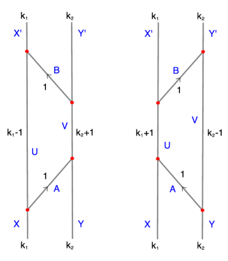
Figure 33: Interface configurations associated to ${\mathcal{F}}{\mathcal{E}}$ (left) and ${\mathcal{E}}{\mathcal{F}}$ (right).

Here, we briefly explain how to obtain (138). Pictorially, the left hand side of this equation is given by the configuration of interfaces depicted on the left of Figure 33. The blue symbols specify the Landau-Ginzburg fields of the respective segments of surface operators. Let ${\mathcal{R}}$ be the polynomial ring in the external variables $(X_{i},X_{i}^{\prime},Y_{i},Y_{i}^{\prime})$ and

$$\widehat{\mathcal{R}}={\mathcal{R}}/(W(X^{\prime}_{1},\ldots,X^{\prime}_{k_{1}})+W(Y^{\prime}_{1},\ldots,Y^{\prime}_{k_{2}})$$ (151)

$$\qquad\qquad\qquad-W(X_{1},\ldots,X_{k_{1}})-W(Y_{1},\ldots,Y_{k_{2}}))$$

the respective hypersurface ring. The $\widehat{\mathcal{R}}$-module corresponding to the matrix factorization on the left hand side of (138) is then given by

$$M=\widehat{\mathcal{R}}_{1}/{\mathcal{J}}\widehat{\mathcal{R}}_{1}\left\{-k_{1}-k_{2}+1\right\}\,,$$ (152)

where

$$\widehat{\mathcal{R}}_{1}=\widehat{\mathcal{R}}\left[A,B,U_{1},\ldots,U_{k_{1}-1},V_{1},\ldots,V_{k_{2}+1}\right]$$ (153)

is obtained by associating the internal variables $(A,B,U_{i},V_{i})$ to $\widehat{\mathcal{R}}$, and ${\mathcal{J}}$ is the ideal in $\widehat{\mathcal{R}}_{1}$ generated by the relations

$$X_{i} = \sigma_{i}(A,U_{1},\ldots,U_{k_{1}-1})$$ (154)

$$X_{i}^{\prime} = \sigma_{i}(B,U_{1},\ldots,U_{k_{1}-1})$$ (155)

$$V_{i} = \sigma_{i}(A,Y_{1},\ldots,Y_{k_{2}})=\sigma_{i}(B,Y_{1}^{\prime},\ldots,Y_{k_{2}}^{\prime})\,.$$ (156)

The module (152) can be recast in the following way. The variables $V_{i}$ can be eliminated by (156). Introducing the new variables

$$\overline{V}_{i}:=Y_{i}-B\overline{V}_{i-1}\,,\quad\overline{V_{0}}=1\,,$$ (157)

the second part of the relations (156) can be rephrased as

$$Y_{i} = \sigma_{i}(B,\overline{V}_{1},\ldots,\overline{V}_{k_{2}})\,,$$ (158)

$$Y_{i}^{\prime} = \sigma_{i}(A,\overline{V}_{1},\ldots,\overline{V}_{k_{2}})\,,$$ (159)

$$(A-B)\overline{V}_{k_{2}} = 0\,.$$ (160)

Thus, we have traded the variables $V_{1},\ldots,V_{k_{2}+1}$ for variables $\overline{V}_{1},\ldots,\overline{V}_{k_{2}}$ and relations (156) for (158), (159) and (160). Defining

$$\widehat{\mathcal{R}}_{2}=\widehat{\mathcal{R}}\left[A,B,U_{1},\ldots,U_{k_{1}-1},\overline{V}_{1},\ldots,\overline{V}_{k_{2}-1}\right]$$ (161)

one obtains

$$M\cong{\widehat{\mathcal{R}}}_{2}[V_{k_{2}}]/{\mathcal{J}}^{\prime}\widehat{\mathcal{R}}_{2}[V_{k_{2}}]\left\{-k_{1}-k_{2}+1\right\}\,,$$ (162)

where ${\mathcal{J}}^{\prime}$ is defined by the relations (154), (155), (158), (159) and (160). Next, one can use (160) to eleminate $\overline{V}_{k_{2}}$:

$$M\cong\underbrace{\widehat{\mathcal{R}}_{2}/{\mathcal{J}}^{\prime\prime}\widehat{\mathcal{R}}_{2}\left\{-k_{1}-k_{2}+1\right\}}_{=:M_{1}}\oplus\underbrace{\widehat{\mathcal{R}}_{2}/((A-B),{\mathcal{J}}^{\prime\prime})\widehat{\mathcal{R}}_{2}\left\{-k_{1}+k_{2}+1\right\}}_{=:M_{2}}\,.$$ (163)

Here ${\mathcal{J}}^{\prime\prime}$ is the ideal in $\widehat{\mathcal{R}}_{2}$ generated by (154), (155), (158) and (159), where $\overline{V}_{k_{2}}$ is set to zero. With $A-B=0$, these equations can be solved on $M_{2}$. One obtains $X_{i}=X_{i}^{\prime}$ and $Y_{i}=Y_{i}^{\prime}$, and (154) can be used to eliminate the $U_{i}$. Only the identity with $i=k_{1}$ in (154) remains and gives rise to the degree $k_{1}$ relation $\sum_{i=0}^{k_{1}}X_{k_{1}-i}(-A)^{i}=0$, which truncates the possible exponents of $A$ ($X_{0}:=1$). Thus,

$$M_{2}\cong\widehat{\mathcal{R}}/{\mathcal{J}}_{2}\widehat{\mathcal{R}}\left\{q^{-k_{1}-k_{2}+1}+q^{-k_{1}-k_{2}+3}+\ldots+q^{k_{1}-k_{2}-1}\right\}\,,$$ (164)

where ${\mathcal{J}}_{2}$ is the ideal in $\widehat{\mathcal{R}}$ generated by the relations

$$0=(X_{i}-X_{i}^{\prime})=(Y_{i}-Y_{i}^{\prime})\,.$$ (165)

Now, $M_{1}$ is symmetric in the roles the variables $(X_{i},X_{i}^{\prime})$ and $(Y_{i},Y_{i}^{\prime})$ play. In particular, it also appears in the module $M^{\prime}$ corresponding to the matrix factorization on the right hand side of equation (138), represented on the right of Figure 33. Indeed,

$$M^{\prime}\cong M_{1}\oplus M_{2}^{\prime}\,,$$ (166)

with

$$M_{2}^{\prime}\cong\widehat{\mathcal{R}}/{\mathcal{J}}_{2}\widehat{\mathcal{R}}\left\{q^{-k_{1}-k_{2}+1}+q^{-k_{1}-k_{2}+3}+\ldots+q^{-k_{1}+k_{2}-1}\right\}\,.$$ (167)

Therefore for $k_{1}\geq k_{2}$

$$M\cong M^{\prime}\oplus\widehat{\mathcal{R}}/{\mathcal{J}}_{2}\widehat{\mathcal{R}}\Big{\{}\underbrace{q^{-k_{1}-+k_{2}+1}+q^{-k_{1}-k_{2}+3}+\ldots+q^{k_{1}-k_{2}-1}}_{[k_{1}-k_{2}]}\Big{\}}\,.$$ (168)

The module $\widehat{\mathcal{R}}/{\mathcal{J}}_{2}\widehat{\mathcal{R}}$ now corresponds to the identity defect in $LG_{k_{1}}\otimes LG_{k_{2}}$, which proves that upon fusion the configurations of interfaces ${\mathcal{E}}$ and ${\mathcal{F}}$ satisfy the quantum $\mathfrak{sl}_{2}$-relations (138).

References

- [1] G. Moore and N. Reshetikhin, A comment on quantum group symmetry in conformal field theory, Nuclear Phys. B 328 (1989), no. 3 557–574.
- [2] S. Cautis, J. Kamnitzer, and A. Licata, Categorical geometric skew Howe duality, Invent. Math. 180 (2010), no. 1 111–159.
- [3] S. Cautis, J. Kamnitzer, and S. Morrison, Webs and quantum skew Howe duality, Math. Ann. 360 (2014), no. 1-2 351–390.
- [4] A. A. Beilinson, G. Lusztig, and R. MacPherson, A geometric setting for the quantum deformation of GL(n), Duke Math. J. 61 (1990), no. 2 655–677.
- [5] I. Grojnowski and G. Lusztig, On bases of irreducible representations of quantum GL(n), in Kazhdan-Lusztig theory and related topics (Chicago, IL, 1989), vol. 139 of Contemp. Math., pp. 167–174. Amer. Math. Soc., Providence, RI, 1992.
- [6] J. Bernstein, I. Frenkel, and M. Khovanov, A categorification of the Temperley-Lieb algebra and Schur quotients of U(sl(2)) via projective and Zuckerman functors, Selecta Math. (N.S.) 5 (1999), no. 2 199–241.
- [7] I. Frenkel, M. Khovanov, and C. Stroppel, A categorification of finite-dimensional irreducible representations of quantum sl(2) and their tensor products, Selecta Math. (N.S.) 12 (2006), no. 3-4 379–431.
- [8] H. Zheng, A geometric categorification of representations of Uq(sl(2)), in Topology and physics, vol. 12 of Nankai Tracts Math., pp. 348–356. World Sci. Publ., Hackensack, NJ, 2008.
- [9] A. D. Lauda, A categorification of quantum sl(2), Adv. Math. 225 (2010), no. 6 3327–3424.
- [10] M. Khovanov and A. D. Lauda, A diagrammatic approach to categorification of quantum groups. I, Represent. Theory 13 (2009) 309–347.
- [11] M. Khovanov and A. D. Lauda, A diagrammatic approach to categorification of quantum groups II, Trans. Amer. Math. Soc. 363 (2011), no. 5 2685–2700.
- [12] M. Khovanov and A. D. Lauda, A diagrammatic approach to categorification of quantum groups. III, Quantum Topol. 1 (2010), no. 1 1–92.
- [13] M. Khovanov, Categorifications from planar diagrammatics, Jpn. J. Math. 5 (2010), no. 2 153–181.
- [14] A. D. Lauda, An introduction to diagrammatic algebra and categorified quantum sl(2), Bull. Inst. Math. Acad. Sin. (N.S.) 7 (2012), no. 2 165–270.
- [15] J. Kamnitzer, Categorification of Lie algebras [d’apres Rouquier, Khovanov-Lauda], Astérisque (2013) Exp. No. 1072. Séminaire Bourbaki. Volume 2012/2013. Exposés.
- [16] R. Rouquier, 2-Kac-Moody algebras, arXiv:0812.5023.
- [17] A. D. Lauda, H. Queffelec, and D. E. V. Rose, Khovanov homology is a skew Howe 2-representation of categorified quantum , Algebr. Geom. Topol. 15 (2015), no. 5 2517–2608.
- [18] H. Queffelec and D. E. V. Rose, The foam 2-category: a combinatorial formulation of Khovanov-Rozansky homology via categorical skew Howe duality, arXiv:1405.5920.
- [19] S. Gukov and E. Witten, Gauge Theory, Ramification, And The Geometric Langlands Program, hep-th/0612073.
- [20] S. Gukov, Gauge theory and knot homologies, Fortsch.Phys. 55 (2007) 473–490, [arXiv:0706.2369].
- [21] S. Gukov and E. Witten, Rigid Surface Operators, Adv. Theor. Math. Phys. 14 (2010) 87–178, [arXiv:0804.1561].
- [22] S. Gukov and E. Witten, Branes and Quantization, Adv. Theor. Math. Phys. 13 (2009) 1, [arXiv:0809.0305].
- [23] I. Brunner and D. Roggenkamp, B-type defects in Landau-Ginzburg models, JHEP 0708 (2007) 093, [arXiv:0707.0922].
- [24] G. Lusztig, Introduction to quantum groups. Birkhäuser, Boston, 1993.
- [25] E. Witten, Quantum Field Theory and the Jones Polynomial, Comm.Math.Phys. 121 (1989) 351–399.
- [26] E. Witten, Gauge Theories and Integrable Lattice Models, Nucl.Phys. B322 (1989) 629.
- [27] E. Witten, Gauge Theories, Vertex Models, and Quantum Groups, Nucl.Phys. B330 (1990) 285.
- [28] H. Wu, A colored homology for links in ., Dissertationes Math. 499 (2014) [0907.0695].
- [29] L. Crane and I. Frenkel, Four-dimensional topological field theory, Hopf categories, and the canonical bases, J. Math. Phys. 35 (1994) 5136–5154, [hep-th/9405183].
- [30] D. Bar-Natan, Khovanov’s homology for tangles and cobordisms, Geom. Topol. 9 (2005) 1443–1499.
- [31] D. Bar-Natan and S. Morrison, The Karoubi envelope and Lee’s degeneration of Khovanov homology, Algebr. Geom. Topol. 6 (2006) 1459–1469.
- [32] M. Mackaay and P. Vaz, The universal sl(3)-link homology, Algebr. Geom. Topol. 7 (2007) 1135–1169.
- [33] E. S. Lee, An endomorphism of the Khovanov invariant, Adv. Math. 197 (2005), no. 2 554–586.
- [34] M. Khovanov, Link homology and Frobenius extensions, Fund. Math. 190 (2006) 179–190.
- [35] B. Gornik, Note on Khovanov link cohomology, math/0402266.
- [36] H. Wu, Generic deformations of the colored sl(N)-homology for links, Algebr. Geom. Topol. 11 (2011), no. 4 2037–2106.
- [37] A. Lobb, A note on Gornik’s perturbation of Khovanov-Rozansky homology, Algebr. Geom. Topol. 12 (2012), no. 1 293–305.
- [38] D. E. V. Rose and P. Wedrich, Deformations of colored sl(N) link homologies via foams, arXiv:1501.0256.
- [39] E. Gorsky, S. Gukov, and M. Stosic, Quadruply-graded colored homology of knots, arXiv:1304.3481.
- [40] M. Khovanov, A categorification of the Jones polynomial, Duke Math. J. 101 (2000) 359–426.
- [41] J. Rasmussen, Khovanov homology and the slice genus, Invent. Math. 182 (2010), no. 2 419–447.
- [42] S. Gukov, Surface Operators, arXiv:1412.7127.
- [43] M. G. Alford, K.-M. Lee, J. March-Russell, and J. Preskill, Quantum field theory of nonAbelian strings and vortices, Nucl.Phys. B384 (1992) 251–317, [hep-th/9112038].
- [44] L. Rozansky, Topological A models on seamed Riemann surfaces, Adv.Theor.Math.Phys. 11 (2007) [hep-th/0305205].
- [45] M. Khovanov and L. Rozansky, Topological Landau-Ginzburg models on the world-sheet foam, Adv. Theor. Math. Phys. 11 (2007), no. 2 233–259.
- [46] W. Lerche, C. Vafa, and N. P. Warner, Chiral Rings in N=2 Superconformal Theories, Nucl.Phys. B324 (1989) 427.
- [47] E. Witten, Phases of N=2 theories in two-dimensions, Nucl.Phys. B403 (1993) 159–222, [hep-th/9301042].
- [48] E. Witten, Solutions of four-dimensional field theories via M theory, Nucl.Phys. B500 (1997) 3–42, [hep-th/9703166].
- [49] A. Gadde, S. Gukov, and P. Putrov, Fivebranes and 4-manifolds, arXiv:1306.4320.
- [50] D. Xie, Higher laminations, webs and N=2 line operators, arXiv:1304.2390.
- [51] D. Xie, Aspects of line operators of class S theories, arXiv:1312.3371.
- [52] M. Bullimore, Defect Networks and Supersymmetric Loop Operators, JHEP 1502 (2015) 066, [arXiv:1312.5001].
- [53] I. Coman, M. Gabella, and J. Teschner, Line operators in theories of class S, quantized moduli space of flat connections, and Toda field theory, arXiv:1505.0589.
- [54] Y. Tachikawa and N. Watanabe, On skein relations in class S theories, arXiv:1504.0012.
- [55] E. Witten, Branes and the dynamics of QCD, Nucl.Phys. B507 (1997) 658–690, [hep-th/9706109].
- [56] E. Frenkel, S. Gukov, and J. Teschner, Surface Operators and Separation of Variables, arXiv:1506.0750.
- [57] L. C. Jeffrey and J. Weitsman, Bohr-Sommerfeld orbits in the moduli space of flat connections and the Verlinde dimension formula, Comm. Math. Phys. 150 (1992), no. 3 593–630.
- [58] S. Agnihotri and C. Woodward, Eigenvalues of products of unitary matrices and quantum Schubert calculus, Math. Res. Lett. 5 (1998), no. 6 817–836.
- [59] P. Belkale, Local systems on P(1)-S for S a finite set, Compositio Math. 129 (2001), no. 1 67–86.
- [60] C. Teleman and C. Woodward, Parabolic bundles, products of conjugacy classes and Gromov-Witten invariants, Ann. Inst. Fourier (Grenoble) 53 (2003), no. 3 713–748.
- [61] N. Ressayre, On the quantum Horn problem, arXiv:1310.7331.
- [62] P. Belkale and S. Kumar, The multiplicative eigenvalue problem and deformed quantum cohomology, arXiv:1310.3191.
- [63] A. Lobb and R. Zentner, The quantum sl(N) graph invariant and a moduli space, Int. Math. Res. Not. IMRN (2014), no. 7 1956–1972.
- [64] J. Grant, The moduli problem of Lobb and Zentner and the colored sl(N) graph invariant, J. Knot Theory Ramifications 22 (2013), no. 10 1350060, 16.
- [65] A. Bertram, Quantum Schubert calculus, Adv. Math. 128 (1997), no. 2 289–305.
- [66] E. Witten, The Verlinde algebra and the cohomology of the Grassmannian, hep-th/9312104.
- [67] S. Gukov and D. Pei, Equivariant Verlinde formula from fivebranes and vortices, arXiv:1501.0131.
- [68] L. Mihalcea, Equivariant quantum Schubert calculus, Adv. Math. 203 (2006), no. 1 1–33.
- [69] M. Eto, Y. Isozumi, M. Nitta, K. Ohashi, K. Ohta, et. al., D-brane configurations for domain walls and their webs, AIP Conf.Proc. 805 (2006) 354–357, [hep-th/0509127].
- [70] M. Eto, T. Fujimori, Y. Isozumi, M. Nitta, K. Ohashi, et. al., Non-Abelian vortices on cylinder: Duality between vortices and walls, Phys.Rev. D73 (2006) 085008, [hep-th/0601181].
- [71] M. Eto, T. Fujimori, M. Nitta, K. Ohashi, and N. Sakai, Domain walls with non-Abelian clouds, Phys.Rev. D77 (2008) 125008, [arXiv:0802.3135].
- [72] H. Queffelec and A. Sartori, Mixed quantum skew Howe duality and link invariants of type A, arXiv:1504.0122.
- [73] D. E. V. Rose and D. Tubbenhauer, Symmetric webs, Jones-Wenzl recursions and q-Howe duality, arXiv:1501.0091.
- [74] P. Ozsvath and Z. Szabo, Holomorphic disks and knot invariants, Adv. Math. 186 (2004) 58–116, [math/0209056].
- [75] J. Rasmussen, Floer homology and knot complements, math/0306378.
- [76] S. Gukov, A. S. Schwarz, and C. Vafa, Khovanov-Rozansky homology and topological strings, Lett.Math.Phys. 74 (2005) 53–74, [hep-th/0412243].
- [77] R. Gopakumar and C. Vafa, M-Theory and Topological Strings-I, hep-th/9809187v1.
- [78] R. Gopakumar and C. Vafa, M-Theory and Topological Strings-II, hep-th/9812127v1.
- [79] M. Aganagic and S. Shakirov, Knot Homology from Refined Chern-Simons Theory, arXiv:1105.5117.
- [80] A. Iqbal and C. Kozcaz, Refined Hopf Link Revisited, arXiv:1111.0525.
- [81] I. Cherednik, Jones polynomials of torus knots via DAHA, arXiv:1111.6195.
- [82] H. Nakajima, Refined Chern-Simons theory and Hilbert schemes of points on the plane, arXiv:1211.5821.
- [83] P. Samuelson, A topological construction of Cherednik’s torus knot polynomials, arXiv:1408.0483.
- [84] E. Witten, Fivebranes and Knots, arXiv:1101.3216.
- [85] A. Haydys, Fukaya-Seidel category and gauge theory, arXiv:1010.2353.
- [86] S. Gukov and J. Walcher, Matrix factorizations and Kauffman homology, hep-th/0512298.
- [87] N. Carqueville and D. Murfet, Computing Khovanov-Rozansky homology and defect fusion, Topology 14 (2014) 489–537, [arXiv:1108.1081].
- [88] H. Fuji, S. Gukov, M. Stosic, and P. Sulkowski, 3d analogs of Argyres-Douglas theories and knot homologies, JHEP 1301 (2013) 175, [arXiv:1209.1416].
- [89] H.-J. Chung, T. Dimofte, S. Gukov, and P. Sulkowski, 3d-3d Correspondence Revisited, arXiv:1405.3663.
- [90] S. Katz, A. Klemm, and C. Vafa, Geometric Engineering of Quantum Field Theories, Nucl. Phys. B497 (1997) [hep-th/9609239].
- [91] T. Dimofte, S. Gukov, and L. Hollands, Vortex Counting and Lagrangian 3-manifolds, Lett.Math.Phys. 98 (2011) 225–287, [arXiv:1006.0977].
- [92] M. Khovanov and L. Rozansky, Matrix factorizations and link homology. II, Geom. Topol. 12 (2008), no. 3 1387–1425, [arXiv:math.QA/0].
- [93] M. Khovanov, sl(3) link homology, Algebr. Geom. Topol. 4 (2004) 1045–1081.
- [94] M. Aganagic, T. Ekholm, L. Ng, and C. Vafa, Topological Strings, D-Model, and Knot Contact Homology, Adv.Theor.Math.Phys. 18 (2014) 827–956, [arXiv:1304.5778].
- [95] H. Fuji and P. Sulkowski, Super-A-polynomial, arXiv:1303.3709.
- [96] M. Khovanov and L. Rozansky, Matrix factorizations and link homology, Fund. Math. 199 (2008), no. 1 1–91, [math/0401268].
- [97] I. Brunner, M. Herbst, W. Lerche, and B. Scheuner, Landau-Ginzburg realization of open string TFT, JHEP 0611 (2006) 043, [hep-th/0305133].
- [98] A. Kapustin and Y. Li, Topological correlators in Landau-Ginzburg models with boundaries, Adv.Theor.Math.Phys. 7 (2004) 727–749, [hep-th/0305136].
- [99] K. Hori and J. Walcher, F-term equations near Gepner points, JHEP 0501 (2005) 008, [hep-th/0404196].
- [100] I. Brunner and D. Roggenkamp, Defects and bulk perturbations of boundary Landau-Ginzburg orbifolds, JHEP 0804 (2008) 001, [arXiv:0712.0188].
- [101] I. Brunner, H. Jockers, and D. Roggenkamp, Defects and D-Brane Monodromies, Adv.Theor.Math.Phys. 13 (2009) 1077–1135, [arXiv:0806.4734].
- [102] S. Gukov and M. Stoi, Homological Algebra of Knots and BPS States, Proc.Symp.Pure Math. 85 (2012) 125–172, [arXiv:1112.0030].
- [103] M. Khovanov and L. Rozansky, Virtual crossings, convolutions and a categorification of the SO(2N) Kauffman polynomial, J. Gökova Geom. Topol. GGT 1 (2007) 116–214.
- [104] Y. Yonezawa, Quantum () link invariant and matrix factorizations,, arXiv:0906.0220.
- [105] R. Elliot and S. Gukov, Exceptional knot homology, arXiv:1505.0163.
- [106] N. M. Dunfield, S. Gukov, and J. Rasmussen, The Superpolynomial for knot homologies, math/0505662.
- [107] S. Cecotti and C. Vafa, On classification of N=2 supersymmetric theories, Commun.Math.Phys. 158 (1993) 569–644, [hep-th/9211097].
- [108] A. Gadde and S. Gukov, 2d Index and Surface operators, JHEP 1403 (2014) 080, [arXiv:1305.0266].
- [109] T. Dyckerhoff and D. Murfet, Pushing forward matrix factorisations, arXiv:1102.2957.
- [110] N. Behr and S. Fredenhagen, Variable transformation defects, Proc. Symp. Pure Math. 85 (2012) 303–312, [arXiv:1202.1678].
- [111] M. Mackaay and Y. Yonezawa, sl(N)-Web categories, arXiv:1306.6242.
- [112] M. Eto, Y. Isozumi, M. Nitta, K. Ohashi, and N. Sakai, Non-Abelian webs of walls, Phys.Lett. B632 (2006) 384–392, [hep-th/0508241].
- [113] M. Shifman and A. Yung, Localization of nonAbelian gauge fields on domain walls at weak coupling (D-brane prototypes II), Phys.Rev. D70 (2004) 025013, [hep-th/0312257].
- [114] M. Eto, Y. Isozumi, M. Nitta, K. Ohashi, and N. Sakai, Webs of walls, Phys.Rev. D72 (2005) 085004, [hep-th/0506135].
- [115] D. Eisenbud, Homological algebra with an application to group representations, Trans. Amer. Math. Soc. 260 (1980) 35–64.