1 Introduction

A significant feature of many gauge theories is the existence of topological solitons which may appear when the gauge and/or global symmetries are spontaneously broken. Monopoles, vortices and domain walls are by now familiar, and have found important applications in vast areas of modern physics, such as cosmology, condensed matter physics and particle physics. From another view point, the topological solitons can be seen as nontrivial solutions of nonlinear differential equations. A direct way to study topological solitons is solving such nonlinear equations exactly. For instance, a beautiful systematic method to construct exact solutions for instantons has been well-established and is widely known as the ADHM construction [1]. This is, however, a special case and for many other types of solitons numerical calculations are needed to study solutions.

The present work concerns the so-called Abrikosov-Nielsen-Olesen (ANO) vortex as the simplest topological soliton with finite energy in the $(1+2)$-dimensional theory. This vortex appears as a topological defect [3] in Ginzburg-Landau theory [2] and may be viewed as a static solution to the equations describing the 1+2 dimensional Abelian Higgs model [4]. In this theory all the vortex features depend on one dimensionless parameter $\lambda=m_{\rm s}/m_{\rm v}$: the ratio of the Higgs boson mass $m_{\rm s}$ to the vector boson mass $m_{\rm v}$. The intervortex force is, roughly speaking, a superposition of an attractive force caused by the Higgs boson and a repulsive force caused by the vector boson as seen in a scalar potential [10]

$$U(R)\simeq\frac{v^{2}}{2\pi}\left(-q_{\rm s}^{2}K_{0}(m_{\rm s}R)+q_{m}^{2}K_{0}(m_{\rm v}R)\right)$$ (1.1)

for a well-separated pair of vortices with a large distance $R$. Here, $q_{\rm s}$ and $q_{m}$ stand for a vortex scalar charge and a magnetic dipole moment, respectively. Therefore the force with the longest correlation length is dominant and the vortices attract (repel) each other for $\lambda<1$ ($\lambda>1$) [6]. The critical coupling $\lambda=1$ is a rather special case where net intervortex forces are exactly canceled thanks to the coincidence of the two coefficients, $q_{\rm s}=q_{\rm m}\equiv 2\pi C_{1}$. From a mathematical viewpoint, the Euler-Lagrange equations reduce to the first order differential equation called the Bogomol’nyi-Prasad-Sommerfield (BPS) equations for vortices saturating Bogomol’nyi bound, whose total energy is quantized as $E_{k}=|k|\pi v^{2}$ with the winding number $k\in\mathbb{Z}$. In this critical case, the constant $C_{1}$ appears, for instance, in a potential for a pair of moving vortices [12]

$$U_{\lambda=1}(R,\vec{u})\simeq\pi v^{2}\times C_{1}^{2}K_{0}(m_{\rm v}R)|\vec{u}|^{2}+{\cal O}(|\vec{u}|^{4})$$ (1.2)

with a relative velocity $\vec{u}$, since only the magnetic field accepts a Lorentz boost and the two forces are not canceled out. Unlike the remarkable cases of instantons and monopoles, no analytic solutions for this BPS equation in flat spacetime have been found even at this critical coupling. Thus only a few quantities are exactly calculable and a detailed study of the vortices, for instance, the calculation of a value of $C_{1}$ requires numerical analysis.

In this paper, to complement the numerical analysis, we propose a simple and straightforward, but new idea for analyzing vortices at critical coupling, where fields are expanded perturbatively with respect to the winding number $k\in\mathbb{Z}$ around its origin $k=0$. To justify this perturbative expansion, (let us call it “small winding-number expansion”), the BPS equations must be extended so that they allow a real winding number $k\in\mathbb{R}$. Since the BPS equations with an infinitesimal winding number $|k|\ll 1$ can be exactly solved, we can systematically perform perturbation calculations without tuning any parameters and this perturbative expansion is supposed to work well as a practical tool. Here, we calculate values of three typical quantities with $\lambda=1$ including $C_{1}$ as the most simple examples to check this idea.

The constant $C_{1}$ has often been calculated in the literature. De Vega & Schaposnik [5] gave a semi-analytical study for axially-symmetric solutions with an arbitrary winding number $k\in\mathbb{Z}_{>0}$, and constructed power-series expansions around a center of a vortex and asymptotic expressions for the opposite side. These two can be determined by only one constant $D_{k}^{k+1}$ for the power-series expansion and $C_{k}$ ($Z_{k}$ in their notation) for the asymptotic expression. Comparing these parameters in a middle region, they obtained the values: $C_{1}=1.7079...$ and $D_{1}^{2}=0.72791...$ . These values now seems to be widely accepted in literature, for instance, $C_{1}=1.7079$ appears in Refs.[7, 11, 13, 15] and also in a standard textbook of Vilenkin & Shellard [8]. However, we encounter a different value for $C_{1}$: $C_{1}=10.58/2\pi\simeq 10.57/2\pi\simeq 1.682\sim 1.684$ which was obtained by Speight [10] about twenty years later than de Vega & Schaposnik [5]. Furthermore, Tong [11] gave the supergravity prediction $C_{1}=8^{1/4}\simeq 1.68179...$ which seems to agree well with Speight’s $C_{1}$. These values also seem to be accepted in literature, for instance, Ref.[12] and another standard textbook by Manton & Sutcliffe [9]. There exists a 1.5 % discrepancy between old and new results.

In Sec.2.6, we shall conclude that the correct value is the old one $C_{1}=1.7079$ by using two different kinds of numerical calculations with higher accuracy. In Sec.4.2.3, we reproduce this value by using the small winding-number expansion to verify its power.

This paper is organized as follows. In Sec.2, we review the BPS vortex in the Abelian-Higgs theory, and define an extended vortex function which allows the winding number of non-integer, as a solution of the BPS equations. There a non-trivial integral formula including the vortex function is derived and three typical constants $C_{\nu},D_{\nu}$ and $S_{\nu}$ for a vortex solution are introduced and their analytical and numerical properties are discussed. In Sec.3 we perform a small winding-number expansion of the vortex function and the three constants using Feynman-like diagrams. Results obtained there are modified in Sec.4, using the Padé approximation to overcome problems with finite convergent radii of the expansions. Summary and discussion are given in Sec.5, and some useful inequalities and details of the calculations are summarized in the Appendices.

2 Review of ANO vortex at critical coupling

2.1 Set up for ANO vortex

The Abrikosov-Nielsen-Olesen (ANO) vortex is an elementary topological soliton in the 2+1 dimensional Abelian-Higgs model

$${\cal L}=-\frac{1}{4e^{2}}F_{\mu\nu}F^{\mu\nu}+\frac{1}{2}({\cal D}_{\mu}\phi)^{*}{\cal D}^{\mu}\phi-V(\phi),$$ (2.1)

where $\phi$ is a complex scalar field, metric is $\eta_{\mu\nu}={\rm diag.}(+1,-1,-1)$ and covariant derivative is ${\cal D}_{\mu}={\partial}_{\mu}+iA_{\mu}$. A scalar potential $V(\phi)$ is of the wine-bottle type

$$V(\phi)=\frac{\lambda^{2}e^{2}}{8}\left(|\phi|^{2}-v^{2}\right)^{2},$$ (2.2)

which has a vacuum $|\phi|=v$ where the $U(1)$ gauge symmetry is spontaneously broken. The Higgs mechanism makes the scalar and the gauge fields massive. Their masses are given by, $m_{\rm s}=\lambda\,ev$, $m_{\rm v}=ev$ respectively. The spontaneously broken $U(1)$ symmetry gives rise to a soliton which is topologically stable object supported by $\pi_{1}(U(1))$, of which element is called a winding number. To require vanishing of the kinetic term $|{\cal D}_{i}\phi|^{2}=0$ at the spatial infinity connects this winding number with the first Chern class

$$\pi_{1}(U(1))=\mathbb{Z}\quad\ni\quad k=-\frac{1}{2\pi}\int d^{2}xF_{12}.$$ (2.3)

This topological defects are called the Abrikosov-Nielsen-Olesen vortex.

In this paper, we take the critical coupling constant, $\lambda=1$, as the simplest model, where the two masses are identical, $m_{\rm v}=m_{\rm s}\equiv m$. Then we can perform the Bogomol’nyi completion of an energy density $\cal H$ for static configurations as

$${\cal H}\big{|}_{\lambda=1} = \frac{1}{2e^{2}}\left\{F_{12}\pm\frac{e^{2}}{2}\left(v^{2}-|\phi|^{2}\right)\right\}^{2}+\frac{1}{2}\left|({\cal D}_{1}\pm i{\cal D}_{2})\phi\right|^{2}$$ (2.4)

$$\quad\mp\frac{v^{2}}{2}F_{12}\pm\frac{i}{2}\epsilon^{ij}{\partial}_{i}\left(\phi{\cal D}_{j}\bar{\phi}\right),$$

and a total mass (tension in higher dimension) of vortices, $T$, has a lower bound

$$T=\int d^{2}x{\cal H}\big{|}_{\lambda=1}\geq\mp\frac{v^{2}}{2}\int d^{2}xF_{12}=\pm\pi v^{2}k.$$ (2.5)

The inequality is saturated by BPS states which satisfy the BPS equations

$$\mp F_{12}=\frac{e^{2}}{2}\left(v^{2}-|\phi|^{2}\right),\quad({\cal D}_{1}\pm i{\cal D}_{2})\phi=0.$$ (2.6)

Without loss of generality we will consider the BPS equations with the upper sign. In order to find general solutions of the BPS equations, it is useful to solve the second equation in Eq. (2.6) at first and, it can be solved with the complex coordinate $z=x_{1}+ix_{2}$ and introducing a smooth real function $\psi_{\rm reg}=\psi_{\rm reg}(z,\bar{z})$

$$A_{\bar{z}}=\frac{i}{2}{\partial}_{\bar{z}}\psi_{\rm reg},\quad\phi=v\,e^{-\frac{\psi_{\rm reg}}{2}}P(z),\qquad P(z)\equiv\prod_{I=1}^{k}(z-z_{I}),$$ (2.7)

where an arbitrary holomorphic function $P(z)$ can be set to be a monic polynomial without loss of generality. Here zeros $\{z_{I}\equiv x^{1}_{I}+ix^{2}_{I}\in\mathbb{C}\}$ of the Higgs field $\phi$ are topological defects and identified as positions of vortices. One of the important features of BPS vortices is that they feel no interactions since the attractive and repulsive force are exactly canceled. So we can put BPS vortices anywhere as many as we like. Note that the smooth field $\psi_{\rm reg}$ must behave as $\psi_{\rm reg}\approx\log|P(z)|^{2}$ at the spatial infinity to obtain a finite energy, it is convenient and more familiar to rewrite $\psi_{\rm reg}$ in terms of a singular field $\psi$,

$$\psi\equiv\psi_{\rm reg}-\log|P(z)|^{2}=-\log\frac{|\phi|^{2}}{v^{2}},$$ (2.8)

so that $\psi$ vanishes at the spatial infinity. With this singular field, then, the first equation in Eq. (2.6) can be rewritten to be, so called, Taubes’ equation

$$-{\partial}_{i}^{2}\psi+m^{2}\left(1-e^{-\psi}\right)=J,$$ (2.9)

with source terms $J$

$$J=J(\vec{x})=4\pi\sum_{I=1}^{k}\delta^{2}(\vec{x}-\vec{x}_{I}).$$ (2.10)

Here we used that the magnetic field can be rewritten as,

$$-F_{12}=2{\partial}_{z}{\partial}_{\bar{z}}\psi_{\rm reg}=\frac{1}{2}\left(\partial_{i}^{2}\psi+J\right)$$ (2.11)

which coincides with Eq.(2.3) and $k$ is the total winding number. Existence and uniqueness of a solution for Taubes’ equation with a given arbitrary $J$ have been established by [14]. With this solution, therefore, we obtain a complete solution for $\phi$ and $A_{i}$. In terms of a solution of $\psi$ and the source $J$, the energy density $\cal H_{\rm BPS}$ for BPS vortices can be rewritten to

$${\cal H}_{\rm BPS}\equiv\frac{v^{2}}{4}\left(J+\partial_{i}^{2}\sigma[\psi]\right),\quad\sigma[\psi]\equiv\psi+e^{-\psi}-1\geq 0,$$ (2.12)

which gives the lower bound in Eq.(2.5). There is, however, no known exact solution for this equation, even in the simplest case with $k=1$.

2.2 Extension of Taubes’ equation and particle description

In a case that $k_{I}$ vortices coincide at $\vec{x}=\vec{x}_{I}$ for each $I$, the source terms are replaced with

$$J=4\pi\sum_{I}k_{I}\delta^{2}(\vec{x}-\vec{x}_{I}),\quad k=\sum_{I}k_{I}.$$ (2.13)

where $k_{I}$ indicates the winding number at $\vec{x}=\vec{x}_{I}$. A request that the winding number $k_{I}$ is positive integer is to give the single-valued Higgs field $\phi$ and Profiles of $\psi$ and the magnetic field in Eq.(2.11) and the energy density in Eq.(2.12) can be calculated without constructing $\phi$. If we omit constructing $\phi$, therefore, we can formally extend Taubes’ equation with the generalized source terms

$$J=4\pi\sum_{I}\nu_{I}\delta^{2}(\vec{x}-\vec{x}_{I}),\quad\nu_{I}\in\{\nu\,|\nu>-1,\nu\in\mathbb{R}\}.$$ (2.14)

Here the winding number $k_{I}$ is renamed $\nu_{I}$ to stress that $\nu_{I}$ can be non-integer and the lower bound of the winding numbers will be discussed in Sec.2.4. A ‘total mass’ of this extended object is formally calculated as

$$T_{\rm BPS}=\int d^{2}x{\cal H_{\rm BPS}}=\pi v^{2}\times\nu,\quad\nu\equiv\sum_{I}\nu_{I},$$ (2.15)

which takes a negative value for $\nu<0$. Integrating the both sides of Taubes’ equation Eq.(2.9) we find the following identity corresponding to Eq.(2.3)

$$\nu=\frac{1}{4\pi}\int d^{2}x\left(\partial_{i}^{2}\psi+J\right)=\frac{m^{2}}{4\pi}\int d^{2}x(1-e^{-\psi}),$$ (2.16)

which is no longer an element of $\pi_{1}(U(1))$. In the rest of this paper, we will study this extended Taubes’ equation with a generalized source term Eq.(2.14) and its solution numerically and analytically. This extension allows us to consider a Taylor expansion of the solution with respect to the winding numbers as discussed in Sec.3, although we are not specially interested in the solution with the winding numbers of non-integer.

Uniqueness of the solution for this extended Taubes’ equation can be easily shown as Appendix A.1. For instance, we know the trivial solution

$$\psi=0\quad{\rm for~{}}\quad J=0.$$ (2.17)

To show existence of the solution for the extended Taubes’ equation is difficult and out of scope of this paper, and we just assume the existence of the solution here. Therefore, the solution of $\psi$ is a function with respect to a coordinate $\vec{x}$, positions of vortices $\{\vec{x}_{I}\}$ and their winding number $\{\nu_{I}\}$, $\psi=\psi(\vec{x},\{\vec{x}_{I},\nu_{I}\})$. Furthermore we assume that the solution is differentiable with respect to $\{\nu_{I}\}$. Under this assumption, we can derive, for each $I$,

$$(-\partial_{i}^{2}+m^{2}e^{-\psi})\frac{\partial\psi}{\partial\nu_{I}}=4\pi\delta^{2}(\vec{x}-\vec{x}_{I})$$ (2.18)

from Taubes equation Eq.(2.9) with the source Eq.(2.14). According to Appendix A.1 the above equation show that the solution $\psi$ is strictly increasing with respect to each $\nu_{I}$, ${\partial}\psi/{\partial}\nu_{I}>0$. In the limit of the vanishing source $J=0$, furthermore we find

$$\lim_{J\to 0}\frac{\partial\psi}{\partial\nu_{I}}=\frac{4\pi}{-\partial^{2}_{i}+m^{2}}\delta^{2}(\vec{x}-\vec{x}_{I})=2K_{0}(m|\vec{x}-\vec{x}_{I}|),\qquad$$ (2.19)

where the modified Bessel function of the second kind $K_{0}(x)$ emerges as a two-dimensional Green’s function. That is, in this limit a vortex solution is exactly solved and treated as a linear combination of free massive particles and for small $|\nu_{I}|\ll 1$ at least, $\psi$ is approximated well everywhere as

$$\psi\approx 2\sum_{I}\nu_{I}K_{0}(m|\vec{x}-\vec{x}_{I}|).$$ (2.20)

This is the starting point of the small winding-number expansion which will be discussed in Sec.3.

In this particle description, it will be convenient to rewrite Taubes’ equation as

$$-\partial_{i}^{2}\psi+m^{2}\psi=J+m^{2}\sigma[\psi],\qquad\sigma[\psi]=\psi^{2}\sum_{n=0}^{\infty}\frac{(-1)^{n}}{(n+2)!}\psi^{n},$$ (2.21)

with $\sigma[\psi]$ as dimensionless self-interaction terms. Then, by applying the Green’s function method to Taubes’ equation, we obtain an integral equation for $\psi$ with Green’s function $G(\vec{x})=K_{0}(m|\vec{x}|)$,

$$\psi(\vec{x}) = 2\sum_{I}\nu_{I}G(\vec{x}-\vec{x}_{I})+m^{2}\int\frac{d^{2}y}{2\pi}G(\vec{x}-\vec{y})\sigma[\psi(\vec{y})].$$ (2.22)

Since $\sigma[\psi]\geq 0$ and $K_{0}(x)>0$ are always hold, we find that the solution of Taubes’ equation must satisfy a fundamental inequality

$$\psi(\vec{x})>2\sum_{I}\nu_{I}K_{0}(m|\vec{x}-\vec{x}_{I}|).$$ (2.23)

2.3 Scaling argument and a physical size of a vortex

Let us consider the following Lagrangian in a two-dimensional Euclidean spacetime

$${\cal L}_{\rm BPS}=-\frac{1}{2}(\partial_{i}\psi)^{2}-m^{2}(\psi+e^{-\psi}-1)+J\psi,\quad$$ (2.24)

which induces Taubes’ equation as an equation of motion of $\psi$, and an action is

$$K=-\int d^{2}x{\cal L}_{\rm BPS}\Big{|}_{\rm solution}+K_{\rm ghost},$$ (2.26)

where $K_{\rm ghost}$ is introduced to cancel UV divergences of the kinetic term and the source term and we set $K_{\rm ghost}$ as, for instance,

$$K_{\rm ghost}=-\int d^{2}x\left(\frac{1}{2}(\partial_{i}\varphi)^{2}+\frac{1}{2}m_{0}^{2}\varphi^{2}-J\varphi\right),\quad$$

$$\varphi(\vec{x})=2\sum_{I}\nu_{I}K_{0}(m_{0}|\vec{x}-\vec{x}_{I}|).$$ (2.27)

After this regularization we can apply the scaling argument to this action. For simplicity, let us consider an axially symmetric case with the source $J=4\pi\nu\delta^{2}(\vec{x})$. Since $K$ is a dimensionless quantity, the dimensional argument tells us

$$0=m^{2}\frac{\partial K}{\partial m^{2}}+m_{0}^{2}\frac{\partial K}{\partial m_{0}^{2}}$$ (2.28)

By using equations of motion for $\psi$ and $\varphi$, derivatives of $K$ with respect to masses can be calculated by

$$m^{2}\frac{\partial K}{\partial m^{2}} = \int d^{2}xm^{2}\left(\psi+e^{-\psi}-1\right)=m^{2}\int d^{2}x\psi-4\pi\,\nu,$$

$$m_{0}^{2}\frac{\partial K}{\partial m_{0}^{2}} = m_{0}^{2}\frac{\partial K_{\rm ghost}}{\partial m_{0}^{2}}=-\int d^{2}x\frac{m_{0}^{2}}{2}\varphi^{2}=-2\pi\nu^{2},$$ (2.29)

where we used Eq.(2.16). Therefore, we find the following formula [18]

$$\int d^{2}x\,\psi=\frac{2\pi}{m^{2}}\times\nu(\nu+2).$$ (2.30)

As we seen the above this exact formula does not come from topological argument, but from the scaling argument. To check numerical calculations we use this formula in this paper. Thanks to this non-trivial identity combining Eq.(2.16), the following integral is calculated as

$$\int d^{2}x|\vec{x}|^{2}\frac{\cal H_{\rm BPS}}{\pi v^{2}}=\frac{1}{8\pi}\int d^{2}x|\vec{x}|^{2}\partial_{i}^{2}\sigma[\psi]=\int\frac{d^{2}x}{2\pi}(\psi+e^{-\psi}-1)=\frac{\nu^{2}}{m^{2}},\quad$$ (2.31)

and a size of the vortex with the positive winding number $\nu>0$ can be naturally defined with the energy density $\cal H_{\rm BPS}$ given in Eq.(2.12) and calculated as,

$$R_{\rm BPS}\equiv\sqrt{2\times\frac{\int d^{2}x|\vec{x}|^{2}{\cal H_{\rm BPS}}}{\int d^{2}x{\cal H}_{\rm BPS}}}=\frac{2\sqrt{\nu}}{m}\quad{\rm for~{}}\nu>0,$$ (2.32)

which turns out to be a key point in Sec.4. It is natural for the scaling argument to determine a typical size of a soliton.

2.4 Axially symmetric solution

Let us consider a single vortex sitting the origin with the winding number $\nu$, that is, we consider a solution with the source term $J=4\pi\nu\delta^{2}(\vec{x})$. Its configuration is axially symmetric and described by a function $\psi=\psi(mr,\nu)$ with respect to a radial coordinate $r=|\vec{x}|$ and the winding number $\nu$. The partial differential equation (2.9), therefore, reduces to an ordinary differential equation

$$\frac{1}{r}\frac{d}{dr}\left(r\frac{d\psi}{dr}\right)=m^{2}(1-e^{-\psi})$$ (2.33)

with the following two boundary conditions

$$\lim_{r\to 0}r\frac{d\psi}{dr}=-2\nu,\quad\lim_{r\to\infty}\psi=0.$$ (2.34)

Even for the non-integer number $\nu$, a set of the differential equation and the boundary conditions defines an unique solution under assumption of its existence. Especially for small $|\nu|\ll 1$, $\psi$ is approximated in the full range of $r\in\mathbb{R}_{>0}$ as

$$\psi\approx E_{1}[\psi]\equiv 2\nu K_{0}(mr),\qquad\lim_{\nu\to 0}\frac{\psi}{\nu}=\lim_{\nu\to 0}\frac{{\partial}\psi}{{\partial}\nu}=\psi_{1}\equiv 2K_{0}(mr).$$ (2.35)

See Fig.1 for some examples of profile functions of $N[\psi]$ which denotes $\psi$ calculated numerically.

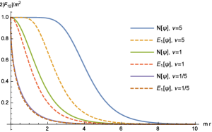
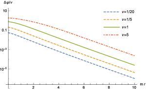
Figure 1: Magnetic flux in the left panel and differences $\Delta\psi=N[\psi]-E_{1}[\psi]$ in the right panel

Here we assume that the solution $\psi$ is smooth with respect to $\nu$ at $\nu=0$. This assumption requires the solution to be extended for the negative winding number $\nu$. Since ${\partial}\psi/{\partial}\nu>0$ as discussed in Sec.2.2, a lower bound of $\nu$ is shown by taking a derivative of the both sides of Eq.(2.30) as

$$0<\int d^{2}x\frac{{\partial}\psi}{{\partial}\nu}=\frac{4\pi}{m^{2}}(\nu+1),$$ (2.36)

that is, there exist no solution of Taubes’ equation with $\nu\leq-1$. We just assume the existence of the solution with $\nu>-1$ in this paper.

Note that we can show the following inequalities although we have no exact solution. Applying the discussion in Appendix.A.1 to Taubes’ equation with the source $J$ in Eq.(2.14), we find the solution $\psi$ must be positive for $\nu>0$ and be negative for $\nu<0$, and Eq.(2.33) tells us that $r\frac{d\psi}{dr}$ is strictly increasing (decreasing) with respect to $r$ for $\nu>0$ ($\nu<0$), and therefore the boundary conditions Eq.(2.34) give lower and upper bounds as,

$$\psi>0,\quad-2\nu<r\frac{d\psi}{dr}<0,\quad {\rm for~{}}\nu>0,$$

$$\psi<0,\quad-2\nu>r\frac{d\psi}{dr}>0,\quad {\rm for~{}}-1<\nu<0.$$ (2.37)

According to Appendix A.1, the following inequality

$$(-\partial_{i}^{2}+m^{2}e^{-\psi})\frac{\partial^{2}\psi}{\partial\nu^{2}}=m^{2}e^{-\psi}\left(\frac{\partial\psi}{\partial\nu}\right)^{2}>0,$$ (2.38)

implies that $\psi$ is a downward-convex function,

$$\frac{\partial^{2}\psi}{\partial\nu^{2}}=\frac{1}{\nu}\frac{{\partial}}{{\partial}\nu}\left(\nu\frac{{\partial}\psi}{{\partial}\nu}-\psi\right)>0.\quad$$ (2.39)

Combining Eq.(2.35) with this fact, we find that $\psi/\nu$ is strictly increasing with respect to $\nu$ and furthermore we obtain

$$\frac{\partial\psi}{\partial\nu}>\frac{\psi}{\nu}>2K_{0}(mr)>0\quad {\rm for~{}}\nu>0,$$

$$0<\frac{\partial\psi}{\partial\nu}<\frac{\psi}{\nu}<2K_{0}(mr)\quad {\rm for~{}}-1<\nu<0.$$ (2.40)

With this axially-symmetric solution $\psi(\vec{x})=\psi(r)$ with $r=|\vec{x}|$, the integral equation Eq.(2.22) reduces to

$$\psi(r) = 2\nu K_{0}(mr)+m^{2}\int_{0}^{\infty}ds\,sG_{\rm F}(r,s)\sigma[\psi(s)],$$ (2.41)

where the reduced Green’s function $G_{\rm F}(r,s)$ takes the following form

$$G_{\rm F}(r,s) = \int\frac{d\theta}{2\pi}K_{0}\left(m\sqrt{r^{2}+s^{2}-2rs\cos\theta}\right)$$ (2.42)

$$= \Theta(r-s)K_{0}(mr)I_{0}(ms)+\Theta(s-r)K_{0}(ms)I_{0}(mr)$$

with the step function $\Theta(x)$ and the modified Bessel function of the first kind $I_{0}(x)$.

2.5 Observable parameters, $C_{\nu},D_{\nu},S_{\nu}$

2.5.1 $D_{\nu}$ and Internal size $R_{\rm in}$

To define the solution $\psi$ of Taubes’ equation even with the positive non-integer winding number $\nu$, we have to consider a behavior of the solution around the core of the vortex seriously. Note that in the massless limit $m\to 0$, Taubes’ equation has a general solution with a positive real arbitrary constant $R_{\rm in}$ as,

$$\lim_{m\to 0}\psi=-\log Y,\quad Y\equiv\left(\frac{r}{R_{\rm in}}\right)^{2\nu}$$ (2.43)

and with the finite mass $m>0$, therefore, $\psi$ can be expanded by $m$ and we find an expansion of $\psi$ around the origin $r=0$ in an unfamiliar form,

$$\psi = -\log Y+\sum_{n=1}^{\infty}F_{n}(Y)(mr)^{2n}$$ (2.46)

$$\approx -2\nu\log(mr)+2D_{\nu}+\left\{\begin{array}[]{cc}\frac{1}{4}(mr)^{2}&{\rm for~{}}\nu>0\vspace{0.5em}\\ -\frac{1}{4}\frac{e^{-2D_{\nu}}}{(1+\nu)^{2}}(mr)^{2(1+\nu)}&{\rm for~{}}-1<\nu<0\end{array}\right.,\qquad\quad$$

where we treated $mr$ and $Y$ as if they were independent of each other, and a function $F_{n}(Y)$ is independent of $m$ and turns out to be a polynomial of order $n$ with respect to $Y$ determined sequentially by solving Taubes’ equation as,

$$F_{1}(Y)=\frac{1}{4}\left(1-\frac{Y}{(1+\nu)^{2}}\right),\quad F_{2}(Y)=\frac{Y}{64}\left(\frac{4}{(2+\nu)^{2}}-\frac{Y}{(1+\nu)^{2}}\right),\cdots$$ (2.47)

which must vanish in the limit $\nu\to 0$ for a finite radius $r$ due to Eq.(2.17). The dimensionless constant $D_{\nu}$ appeared in the expansion is related to $R_{\rm in}$ as

$$D_{\nu}=\nu\log(mR_{\rm in}).$$ (2.49)

Therefore the expansion of $\psi$ can be defined by a pair of parameters $\{\nu,R_{\rm in}\}$. The uniqueness of the solution with a given $\nu$ means, however, that to satisfy the boundary condition at the spatial infinity, the constant $R_{\rm in}$ must take a certain value corresponding to each value of $\nu$, that is, a function $R_{\rm in}=R_{\rm in}(\nu)$, otherwise a function defined by the expansion always glows up at a large $r$. In Appendix A.2 this feature is analytically discussed and at the present we find a pair of lower and upper bounds of $R_{\rm in}$ as

$$\frac{2\sqrt{\nu+1}}{m}>R_{\rm in}>\frac{2}{m}\sqrt{\frac{\nu}{e}}\qquad{\rm for~{}}\nu>0.$$ (2.50)

According to Eq.(2.40) $R_{\rm in}$ and $D_{\nu}/\nu$ turn out to be strictly increasing functions with respect to $\nu$ and take values at $\nu=0$

$$\lim_{\nu\to 0}\frac{D_{\nu}}{\nu} = \lim_{r\to 0}(K_{0}(r)+\log r)=\log 2-\gamma\approx 0.115932,$$

$$\lim_{\nu\to 0}R_{\rm in} = \frac{2e^{-\gamma}}{m}\approx\frac{1.12292}{m},\qquad$$ (2.51)

with Euler’s gamma $\gamma$. In Fig.2, we plot a profile of $D_{\nu}/\nu$.

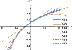
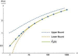
Figure 2: Profile of $D_{\nu}$ for the full range of $\nu$. Numerical Data $N_{\rm sht}[D_{\nu}]$ are plotted by dots. Dashed lines in the left panels describe $E_{n}[D_{\nu}]$ given in Sec.3. Dashed lines in the right panel give the bounds given in Eq.(2.50). $\widehat{P}_{2}[D_{\nu}],\widehat{P}_{6}[D_{\nu}]$ plotted by a solid line are defined in Sec.4.

Note that there is an another way to calculate $D_{\nu}$ using the integral form Eq.(2.41) as,

$$D_{\nu}=\lim_{r\to 0}\left(\frac{\psi}{2}+\nu\log(mr)\right)=\nu(\log 2-\gamma)+\frac{m^{2}}{2}\int_{0}^{\infty}dssK_{0}(ms)\sigma[\psi(s)].$$ (2.52)

These different two definitions of $D_{\nu}$ will be used to double-check numerical calculations of $D_{\nu}$.

Since the axially symmetric vortex solution we consider has the only one mass parameter $m$, we expect that the dimensionfull parameter $R_{\rm in}$ controlling a profile of the solution should be the same order of the vortex size $R_{\rm BPS}$ given in Eq.(2.32). Thanks to Eq.(2.50), roughly speaking, we find actually $R_{\rm BPS}\approx R_{\rm in}$ for large $\nu$. We call $R_{\rm in}$ an internal size. On the other hand $D_{\nu}$ is directly related to a value of the action $K$ with $J=4\pi\nu\delta^{2}(\vec{x})$ in the previous subsection. In the same way of Eq.(2.29), we can calculate a derivative of $K$ with respective to $\nu$,

$$\frac{\partial K}{\partial\nu}=-4\pi\times\lim_{r\to 0}\left(\psi-\varphi\right)=8\pi\nu\log\left(\frac{m}{m_{0}}\right)-8\pi\left(D_{\nu}-\nu(\log 2-\gamma)\right)$$ (2.53)

and by setting the mass of the ghost $m_{0}$ to be $m_{0}=2e^{-\gamma}m$, we obtain the following simple relations,

$$D_{\nu}=-\frac{1}{8\pi}\frac{dK}{d\nu},\quad K=-8\pi\int_{0}^{\nu}dyD_{y}.$$ (2.54)

2.5.2 Scalar charge $C_{\nu}$

Let us take $m$ large conversely, that is, consider a infrared region $r\gg R_{\rm in}\approx 2\sqrt{\nu}/m$. There, an asymptotic behavior of $\psi$ can be treated as a fluctuation of a free massive scalar field around the vacuum. Due to the axial symmetry, such a fluctuation is written with a certain constant $C_{\nu}\in\mathbb{R}_{>0}$ as

$$\psi\approx 2C_{\nu}K_{0}(mr).$$ (2.55)

There is the similarity between this asymptotic form and the form of Eq.(2.35) and the uniqueness of the solution of Taubes’ equation indicates that the two constants $C_{\nu}$ and $\nu$ are in one-to-one correspondence. Actually, to satisfy the boundary condition at the origin $r=0$, the constant $C_{\nu}$ must be a function with respect to $\nu$ and according to Eq.(2.17), Eq(2.19) and Eq(2.39) we find

$$\lim_{\nu\to 0}C_{\nu}=0,\quad\lim_{\nu\to 0}\frac{dC_{\nu}}{d\nu}=1,\quad\frac{d^{2}C_{\nu}}{d\nu^{2}}>0.$$ (2.56)

These property tell us that $C_{\nu}/\nu$ is strictly increasing with respect to $\nu$ and a lower bound of $C_{\nu}$ is given as $C_{\nu}>\nu$. A profile of this function is shown in Fig.3.

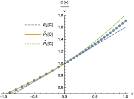
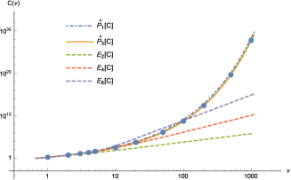
Figure 3: Profile of $C_{\nu}$ for small $\nu$ in the left panel and for large $\nu$ in the right panel. Numerical Data $N_{\rm sht}[C_{\nu}]$ are plotted by dots. Dashed lines in the both panels describe approximants of the order $n$, $E_{n}[C_{\nu}]$, in terms of the winding-number expansion discussed in Sec.3. $\widehat{P}_{3}[C_{\nu}]$ plotted by a solid line and $\widehat{P}_{1}[C_{\nu}]$ plotted by a dot-dash-line are defined in Sec.4.

According to the integral equation Eq.(2.41), $C_{\nu}$ can be calculated by

$$C_{\nu}=\lim_{r\to\infty}\frac{\psi}{2K_{0}(mr)}=\nu+\frac{m^{2}}{2}\int_{0}^{\infty}dssI_{0}(ms)\sigma[\psi(s)].$$ (2.57)

Bringing this identity back, we can remove the explicit $\nu$-dependence from the integral equation Eq.(2.41) as

$$\psi(\vec{x})=2C_{\nu}K_{0}(mr)-\int_{0}^{\infty}ds\,sG_{\rm ad}(r,s)\sigma[\psi(s)],$$ (2.58)

with an ‘advanced’ Green’s function

$$G_{\rm ad}(r,s)=\Theta(s-r)\left\{K_{0}(mr)I_{0}(ms)-I_{0}(mr)K_{0}(ms)\right\}\geq 0.$$ (2.59)

Using this integral equation Eq.(2.58), the asymptotic behavior in Eq.(2.55) is modified as

$$\psi=2C_{\nu}K_{0}(mr)-2C_{\nu}^{2}\int_{0}^{\infty}ds\,sG_{\rm ad}(r,s)K_{0}(ms)^{2}+{\cal O}(e^{-3mr}).$$ (2.60)

Thanks to these two different forms of the integral equations for $\psi$ Eq.(2.41) and Eq.(2.58), we find lower and upper bounds as

$$2\nu K_{0}(mr)<\psi<2C_{\nu}K_{0}(mr).$$ (2.61)

A one of purposes of this paper is to confirm the true value of $C_{1}$.

2.5.3 Total scalar potential $S_{\nu}$

Finally let us consider the following definite integral

$$S_{\nu}=\frac{m^{2}}{2}\int\frac{d^{2}x}{2\pi}(1-e^{-\psi})^{2},$$ (2.62)

which is dimensionless and proportional to a total potential energy of the Abelian-Higgs model at critical coupling,

$$S_{\nu} = \frac{\lambda}{E_{1}}\frac{{\partial}E_{\nu}}{{\partial}\lambda}\Big{|}_{\lambda=1}=\frac{2}{E_{1}}\int d^{2}xV(\phi)\Big{|}_{\lambda=1,\rm sol},$$ (2.63)

This quantity with $\nu>0$ satisfies

$$0\quad<\quad S_{\nu}\quad<\quad\frac{m^{2}}{2}\int\frac{d^{2}x}{2\pi}(1-e^{-\psi})=\nu,$$ (2.64)

and according to Eq.(2.17) and Eq.(2.19) we find

$$\lim_{\nu\to 0}S_{\nu}=\lim_{\nu\to 0}\frac{dS_{\nu}}{d\nu}=0,\quad\lim_{\nu\to 0}\frac{d^{2}S_{\nu}}{d\nu^{2}}=2.$$ (2.65)

Thanks to Eq.(2.40) we find that $S_{\nu}$ is also an increasing function with respect to $\nu$ and according to the profile of $S_{\nu}$ shown in Fig.4 an ‘energy’ per an unit winding number $S_{\nu}/\nu$ is also an increasing function with respect to $\nu$, and this property gives

$$S_{\nu_{1}+\nu_{2}}>S_{\nu_{1}}+S_{\nu_{2}}.$$ (2.66)

This inequality is consistent with the well known property of type II (type I) vortices, that is, intervortex forces are repulsive (attractive) for the coupling $\lambda>1(\lambda<1)$.

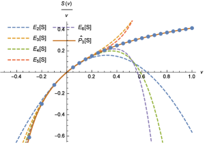
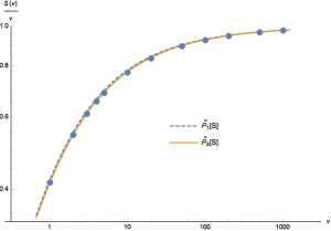
Figure 4: Profile of $S_{\nu}$ for the full range of $\nu$. Numerical Data $N_{\rm sht}[S_{\nu}]$ are plotted by dots. Dashed lines in the left panels describe $E_{n}[S_{\nu}]$ given in Sec.3. $\widehat{P}_{3}[S_{\nu}]$ plotted by a solid line and $\widehat{P}_{1}[S_{\nu}]$ plotted by a dashed-line are defined in Sec.4.

2.6 Numerical Data

We numerically calculate values of $C_{\nu},D_{\nu},S_{\nu}$ in most of the range of $\nu$ as $\nu=1/20,1/10,\cdots,500,1000$ using mainly the shooting method. These data are listed in Table.1.

$\nu$	$C_{\nu}$	$D_{\nu}$	$R_{\rm in}$	$S_{\nu}$
1/20	0.05152300	0.007221252	1.155375	0.002320344⋆
1/10	0.1061386	0.01714170	1.186986	0.008668711⋆
1/5	0.2249350	0.04429221	1.247899	0.03070642⋆
1/2	0.6633334	0.1736933	1.415364	0.1444002⋆
1	1.707864	0.5053608	1.657584	0.4153533
2	5.336582	1.443305	2.057831	1.085081
3	11.86421	2.615596	2.391367	1.832041
4	22.61080	3.948209	2.683313	2.619544
5	39.31961	5.402536	2.946174	3.432922
10	317.5504	13.88300	4.008030	7.704638
20	5424.053	34.27687	5.550253	16.68079
50	1284274.	107.9305	8.659094	44.65765
100	5.455139$\times 10^{8}$	250.0538	12.18905	92.38242
200	2.607156$\times 10^{12}$	568.9475	17.19704	189.1678
500	4.568733$\times 10^{19}$	1650.717	27.15154	482.7929
1000	6.065189$\times 10^{27}$	3647.519	38.37932	975.6104

Table 1: Numerical Data of $C_{\nu}$, $D_{\nu}(R_{\rm in})$ and $S_{\nu}$. All data are sufficiently stable values and we double-checked them except for data added stars.

We will denote these data as $N_{\rm sht}[C_{\nu}],N_{\rm sht}[D_{\nu}]$ and $N_{\rm sht}[S_{\nu}]$ for $C_{\nu},D_{\nu},S_{\nu}$ respectively. In Sec.4, we use these data as references to show how the winding-number expansion introduced in Sec.3 works well. The other purpose of this subsection is to settle the problem on the numerical value of $C_{1}$. We need, therefore, numerical calculations with high accuracy. To show accuracy of our numerical data to readers, let us enter into details of the numerical calculations we performed.

Note that there exist two kinds of strategies in the shooting method and we observe a big difference in usability between them. We calculate numerical solutions of $\psi$ in a region $\{r\,|\epsilon\leq r\leq L\}$ where we set $m=1$ and take $\epsilon=10^{-2n+1}$ and $L=2\sqrt{\nu}+p\log 10$ with $p,n=8\sim 9$ referring to the flux size $R_{\rm flux}$ given in Eq.(2.32). The first strategy is to take $r=\epsilon$ as the initial point of the calculation and fine-tune the parameter $D_{\nu}$ so that a profile of $\psi$ satisfies the boundary condition at $r=L$ and read $C_{\nu}$ from a profile of $\psi$ at $r=L$. Since the initial conditions are given by a pair $\{\nu,D_{\nu}\}$, an incorrect pair always makes a profile function blow up at large $r$. The second one is to take $r=L$ as the initial point and fine-tune the parameter $C_{\nu}$ so that $\nu=-(r\psi^{\prime}/2)$ at $r=\epsilon$ and read $D_{\nu}$ at $r=\epsilon$. In this strategy the profile function is controlled by the only one initial parameter $C_{\nu}$ which is related to $\nu$ in one-to-one correspondence thanks to $dC_{\nu}/d\nu>1$. With the sufficiently large $L$, therefore, a profile function with an arbitrary $C_{\nu}$ always gives a certain solution corresponding to a certain $\nu$, without the profile blowing up, and thus this strategy gives a function $\nu=f(C_{\nu})$. Thanks to this property, it is easy to create a computer program for tuning $C_{\nu}$ automatically with a given $\nu$ and arbitrary precision. We take the second strategy in this paper although the first strategy was taken in Speight’s paper [10].

As we explained above, numerical data $N_{\rm sht}[C_{\nu}],N_{\rm sht}[D_{\nu}]$ for $C_{\nu},D_{\nu}$ are directly obtained. To double-check those data, we also use the integral formulas Eq.(2.57) and Eq.(2.52) for $C_{\nu},D_{\nu}$ respectively, to obtain different data $N_{\rm sht}^{\prime}[C_{\nu}],N_{\rm sht}^{\prime}[D_{\nu}]$. We regard $|N^{\prime}_{\rm sht}[X]/N_{\rm sht}[X]-1|$ with $X=C_{\nu},D_{\nu}$, as errors of these data and plot them in the right panel of Fig.5. For instance, we obtain as double-checked numbers,

$$N_{\rm sht}[C_{1}] = 1.707864175$$

$$N_{\rm sht}[D_{1}] = 0.505360825378$$ (2.68)

for $\nu=1$ and the numerical data listed in Table.1 have been double-checked in this sense. Therefore we conclude that the numerical result $C_{1}=1.7079$ given by de Vega and Schaposnik is correct. Thanks to the non-trivial identity in Eq.(2.30), we can estimate accuracy of the profile functions itself by calculating the following quantity

$$\delta=\left|\frac{1}{\nu(\nu+2)}\left\{\int_{\epsilon}^{L}drrN[\psi]+2N[C_{\nu}]\int_{L}^{\infty}drrK_{0}(r)\right\}-1\right|,$$ (2.69)

and we plotted this in the right panel of Fig.5. Note that we observe that the precision of $N_{\rm sht}[C_{\nu}]$ generally get worse than those of $\delta,D_{\nu}$ as shown in Fig.5. The precision of calculations in Speight’s paper seems to be less than six digits and we guess that his result $C_{1}\approx 1.683$ has an error of ${\cal O}(10^{-2})\sim{\cal O}(10^{-3})$ which is consistent with the other numerical results including ours.

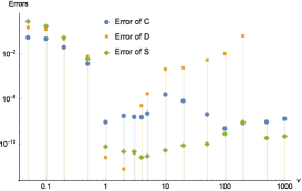
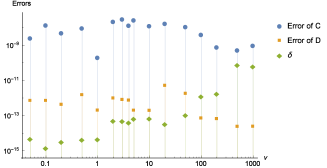
Figure 5: Estimated numerical errors: The left panel plots errors of numerical data calculated by the relaxation method from those calculated by the shooting method as, $|N_{\rm rlx}[X]/N_{\rm sht}[X]-1|$ with $X=C_{\nu},D_{\nu},S_{\nu}$. The right panel plots errors of numerical data in terms of the shooting method itself as, $|N^{\prime}_{\rm sht}[C_{\nu}]/N_{\rm sht}[C_{\nu}]-1|,|N^{\prime}_{\rm sht}[D_{\nu}]/N_{\rm sht}[D_{\nu}]-1|$ and $\delta$.

We obtain also a stable numerical value of $S_{1}$ with long digits

$$N_{\rm sht}[S_{1}]=0.4153533072562,$$ (2.70)

by the shooting method. To perform double check of the values of $S_{\nu}$, we also use the relaxation method as the other numerical calculation. In the relaxation method, we introduce a relaxation time $\tau$ and extend $\psi(\vec{x})$ to be dependent on $\tau$, $\psi=\psi(\vec{x},\tau)$, and modify the equations of motion by adding a friction term $\partial\psi/\partial\tau$ with an appropriate signature. With an appropriate initial function of $\psi$, $\psi(r,\tau=0)=2\nu K_{0}(r)$ for instance, this friction term defines the time evolution of $\psi$ and decreases an ‘energy’ of this system defined in Eq.(2.26). In principle, therefore, the true solution could be obtained with an infinite $\tau$ as $\psi(r)=\lim_{\tau\to\infty}\psi(r,\tau)$. As larger $\tau$, we will get better accuracy in many cases. In reality, beyond a certain finite $\tau$, we observe stability of values of the observables with small noises, since those accuracy can not be better than the calculation accuracy. For instance we stopped the time evolutions at $\tau\approx 4\times 10^{4}$. The relaxation method is convenient and powerful to solve (simultaneous) nonlinear (partial) differential equations numerically. We need no fine-tuning of any parameters there. In the simple system we are considering, however, the shooting method is more powerful to get precision. Generally speaking, numerical data $N_{\rm rlx}[X]$ for $X=C_{\nu},D_{\nu},S_{\nu}$ calculated by the relaxation method get worse precision as shown as Fig.5. We find $|N_{\rm rlx}[S_{1}]/N_{\rm sht}[S_{1}]-1|\approx 5\times 10^{-11}$ which is guessed to be mainly an error of $N_{\rm rlx}[S_{1}]$. We also get $N_{\rm rlx}[C_{1}]=1.707864188\dots$ and $N_{\rm rlx}[D_{1}]=0.5053608253753\dots$ again.

3 Small Winding-Number Expansion

In the paper[5], de Vega and Schaposnik calculated $C_{1}$ and $D_{1}$ by a semi-analytical study. Their strategy was essentially as follows. Let us divide the integrals in Eq.(2.52) and Eq.(2.57) as

$$\int_{0}^{\infty}=\int_{0}^{b}+\int_{b}^{\infty},\quad{\rm with~{}}b\approx R_{\rm BPS}.$$ (3.1)

The former integral is calculated by inserting the expansion Eq.(2.46) which depends on $D_{\nu}$ and the latter is calculated by the expansion Eq.(2.60) which depends on $C_{\nu}$. Then we obtain simultaneous equations for $C_{\nu}$ and $D_{\nu}$, and thus, approximate the values of $C_{\nu}$, $D_{\nu}$ as their solution.

In this section we will give a different expansion of the solution $\psi$ using Eq.(2.41) and calculate them more straightforwardly and more systematically.

3.1 $\nu$-expansion of the vortex function $\psi$

In the normal case, we can not define an expansion of $\psi$ with respect to the winding number as a topological quantum number. In the previous section, we relax the winding number $\nu$ from an integer to a real number and assume smoothness at $\nu=0$, and thus, we can consider a Taylor expansion of the solution for $\psi$ with respect to the winding number as, with Eq.(2.17)

$$\psi=\sum_{n=1}^{\infty}\nu^{n}\psi_{n}.$$ (3.2)

Since the approximate solution $E_{1}[\psi]=\nu\psi_{1}$ in Eq.(2.35) satisfies the boundary conditions Eq.(2.34) and has the same asymptotic form as Eq.(2.55) for an arbitrary $\nu$, we expect that the following finite series of order $n$

$$E_{n}[\psi]\equiv\sum_{m=1}^{n}\nu^{m}\,\psi_{m}$$ (3.3)

gives a good approximation and becomes better as the larger order $n$. Here, a higher-order coefficient $\psi_{n}$ for $n\geq 2$ can be sequentially calculated by expanding the integral equation in Eq.(2.22), or Eq.(2.41) for the axially symmetric case, with the first approximant $E_{1}[\psi]$, as

$$\psi_{n}(\vec{x})=m^{2}\int\frac{d^{2}y}{2\pi}G(\vec{x}-\vec{y})\sigma_{n}(\vec{y}),\quad\sigma[\psi]=\sum_{n=2}^{\infty}\nu^{n}\sigma_{n}$$ (3.4)

where expansion coefficients $\sigma_{n}=\sigma_{n}(\vec{x})$ in the interaction terms $\sigma[\psi]$ are

$$\sigma_{2}=\frac{1}{2}\psi_{1}^{2},\quad\sigma_{3}=-\frac{1}{6}\psi_{1}^{3}+\psi_{1}\psi_{2},\quad\cdots.$$ (3.5)

Let us call this Taylor expansion a small winding-number expansion , or simply, a $\nu$-expansion. Note that in this expansion the winding number $\nu$ is fixed and higher order corrections have no logarithmic singularity as

$$\lim_{r\to 0}r\frac{d\psi_{n}}{dr}=0\quad{\rm for~{}}n\geq 2.$$ (3.6)

The absence of the solution for $\nu\leq-1$ shown in Eq.(2.36) might indicate that a radius of convergence for the $\nu$-expansion of $\psi$ is less than 1. In Sec.4, we will discuss that this fact is not a big problem.

We can perform calculations of the $\nu$-expansion of $\psi$ with the familiar technic using Feynman diagrams. The $\nu$-expansion of $\psi(\vec{x})$ is given concretely as

$$\psi(\vec{x}) = 2\nu\times{\begin{minipage}[h]{108.405pt} \includegraphics[width=433.62pt,keepaspectratio={true}]{prop.eps} \end{minipage}}+\frac{1}{2}(2\nu)^{2}\times{\begin{minipage}[h]{86.72267pt} \includegraphics[width=433.62pt,keepaspectratio={true}]{psv3.eps} \end{minipage}}$$ (3.7)

$$+(2\nu)^{3}\times\left\{\frac{1}{2}{\begin{minipage}[h]{86.72267pt} \includegraphics[width=433.62pt,keepaspectratio={true}]{psv3pv3.eps} \end{minipage}}-\frac{1}{6}{\begin{minipage}[h]{65.04034pt} \includegraphics[width=433.62pt,keepaspectratio={true}]{psv4.eps} \end{minipage}}\right\}$$

$$+(2\nu)^{4}\times\left\{\frac{1}{2}{\begin{minipage}[h]{86.72267pt} \includegraphics[width=433.62pt,keepaspectratio={true}]{psv3pv3pv3.eps} \end{minipage}}+\frac{1}{8}{\begin{minipage}[h]{86.72267pt} \includegraphics[width=433.62pt,keepaspectratio={true}]{psv3av3pv3.eps} \end{minipage}}\right.$$

$$\qquad\left.-\frac{1}{6}{\begin{minipage}[h]{86.72267pt} \includegraphics[width=433.62pt,keepaspectratio={true}]{psv3pv4.eps} \end{minipage}}-\frac{1}{4}{\begin{minipage}[h]{86.72267pt} \includegraphics[width=433.62pt,keepaspectratio={true}]{psv4pv3.eps} \end{minipage}}+\frac{1}{24}{\begin{minipage}[h]{65.04034pt} \includegraphics[width=433.62pt,keepaspectratio={true}]{psv5.eps} \end{minipage}}\right\}$$

$$+{\cal O}(\nu^{5}),$$

using conventions for Feynman diagrams,

$$G(\vec{x})=K_{0}(m|\vec{x}|)={\begin{minipage}[h]{130.08731pt} \includegraphics[width=433.62pt,keepaspectratio={true}]{prop.eps} \end{minipage}},\quad m^{2}\int\frac{d^{2}y}{2\pi}G(\vec{x}-\vec{y})G(\vec{y})^{2}={\begin{minipage}[h]{86.72267pt} \includegraphics[width=433.62pt,keepaspectratio={true}]{psv3.eps} \end{minipage}}.$$ (3.8)

Here diagrams of the order $n$ have $n$ external legs coming from the point-like vortex at the origin $\vec{x}=\vec{0}$.

3.2 $E_{n}[C_{\nu}]$

Let us approximate $C_{\nu}$ analytically by using the $\nu$-expansion,

$$C_{\nu}=\sum_{n=1}^{\infty}c_{n}\nu^{n},\quad c_{1}=1.$$ (3.9)

In principle, its coefficients $c_{n}$ can be obtained by taking the $\nu$-expansions of the both sides of Eq.(2.57) and inserting $\psi_{n}$ obtained in Eq.(3.7) into the right hand side. Comparing Eq.(2.41) and Eq.(2.57), however, we find that the coefficient $c_{n}$ can be calculated by only replacing the propagator with $I_{0}(m|\vec{x}|)$ as

$$\psi_{n}(\vec{x})={\begin{minipage}[h]{86.72267pt} \includegraphics[width=433.62pt,keepaspectratio={true}]{psgeneral.eps} \end{minipage}}\quad\Rightarrow\quad c_{n}=\frac{1}{2}{\begin{minipage}[h]{86.72267pt} \includegraphics[width=433.62pt,keepaspectratio={true}]{Cgeneral.eps} \end{minipage}}$$ (3.10)

where the triangle symbol stands for

$$I_{0}(m|\vec{x}|)={\begin{minipage}[h]{65.04034pt} \includegraphics[width=433.62pt,keepaspectratio={true}]{I0.eps} \end{minipage}}.$$ (3.11)

For instance, coefficients $c_{2},c_{3}$ are calculated as

$$c_{2} = {\begin{minipage}[h]{65.04034pt} \includegraphics[width=433.62pt,keepaspectratio={true}]{Iv3.eps} \end{minipage}}=\int_{0}^{\infty}drr\,I_{0}(r)K_{0}(r)^{2}=\frac{\pi}{3\sqrt{3}}\approx 0.604600,$$

$$c_{3} = 2{\begin{minipage}[h]{78.04842pt} \includegraphics[width=433.62pt,keepaspectratio={true}]{Iv3pv3.eps} \end{minipage}}-\frac{2}{3}{\begin{minipage}[h]{65.04034pt} \includegraphics[width=433.62pt,keepaspectratio={true}]{Iv4.eps} \end{minipage}}$$ (3.12)

$$= 2\times\frac{11}{432}\pi^{2}-\frac{2}{3}\times\frac{\pi^{2}}{16}=\frac{\pi^{2}}{108}\approx 0.0913852.$$

See Appendix B for details. Finally we obtain

$$C_{\nu} = \nu+\frac{\pi}{3\sqrt{3}}\nu^{2}+\frac{\pi^{2}}{108}\nu^{3}+0.0126799\nu^{4}$$ (3.13)

$$\quad-0.0013557(41)\nu^{5}+0.000781(22)\nu^{6}+{\cal O}(\nu^{7}),$$

which gives a finite series $E_{n}[C_{\nu}]$ as an approximant of order $n$

$$E_{n}[C_{\nu}]=\sum_{k=1}^{n}c_{k}\,\nu^{k}.$$ (3.14)

As shown in Fig.6, we observe that as the order $n$ is larger, an error of $E_{n}[C_{1}]$, that is, $|E_{n}[C_{1}]/N_{\rm sht}[C_{1}]-1|$ is smaller. The sixth order approximant for $\nu=1$, $E_{6}[C_{1}]$, gives a quite nice value near to the numerical value $N_{\rm sht}[C_{1}]$ in Eq.(2.68) as

$$E_{6}[C_{1}]=1.70809\dots,\quad\left|\frac{E_{6}[C_{1}]-N_{\rm sht}[C_{1}]}{N_{\rm sht}[C_{1}]}\right|\approx 1.0\times 10^{-4}.$$ (3.15)

Unfortunately the accuracy of this value is worse than that of the value $C_{1}\approx 1.7079$ given by de Vega and Schaposnik. According to Fig.6 a radius of convergence of the infinite series, $\nu_{\rm c}$, is obviously finite and smaller than ten, $\nu_{\rm c}<10$ and we can not judge whether $\nu_{\rm c}$ is larger than one or not. In Sec.4, we will overcome these problems.

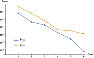
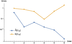
Figure 6: Errors of the $n$-th order approximants $E_{n}[C_{1}]$ and $\widehat{P}_{n}[C_{1}]$ in the left panel, and $E_{n}[C_{10}]$ and $\widehat{P}_{n}[C_{10}]$ in the right panel. $\widehat{P}_{n}[C_{\nu}]$ will be defined in Sec.4

3.3 $E_{n}[D_{\nu}]$

Next, let us consider the $\nu$-expansion of $D_{\nu}$,

$$D_{\nu}=\sum_{n=1}^{\infty}d_{n}\nu^{n},\quad d_{1}=\log 2-\gamma.$$ (3.16)

According to Eq.(2.52), the expansion coefficient $d_{n}$ for $n\geq 2$, is calculated by reducing diagrams in Eq.(3.7) as,

$$\psi_{n}(\vec{x})={\begin{minipage}[h]{86.72267pt} \includegraphics[width=433.62pt,keepaspectratio={true}]{psgeneral.eps} \end{minipage}}\quad\Rightarrow\quad d_{n}=\frac{1}{2}{\begin{minipage}[h]{86.72267pt} \includegraphics[width=433.62pt,keepaspectratio={true}]{Dgeneral.eps} \end{minipage}}.$$ (3.17)

We find therefore, by performing integrals numerically,

$$D_{\nu} = (\log 2-\gamma)\nu+\nu^{2}\times{\begin{minipage}[h]{65.04034pt} \includegraphics[width=433.62pt,keepaspectratio={true}]{v3.eps} \end{minipage}}+\nu^{3}\times\left\{2{\begin{minipage}[h]{78.04842pt} \includegraphics[width=433.62pt,keepaspectratio={true}]{v3pv3.eps} \end{minipage}}-\frac{2}{3}{\begin{minipage}[h]{65.04034pt} \includegraphics[width=433.62pt,keepaspectratio={true}]{v4.eps} \end{minipage}}\right\}$$ (3.18)

$$+\nu^{4}\times\left\{5{\begin{minipage}[h]{86.72267pt} \includegraphics[width=433.62pt,keepaspectratio={true}]{v3pv3pv3.eps} \end{minipage}}-\frac{10}{3}{\begin{minipage}[h]{86.72267pt} \includegraphics[width=433.62pt,keepaspectratio={true}]{v3pv4.eps} \end{minipage}}+\frac{1}{3}{\begin{minipage}[h]{86.72267pt} \includegraphics[width=433.62pt,keepaspectratio={true}]{v5.eps} \end{minipage}}\right\}+{\cal O}(\nu^{5})$$

$$= 0.115932\nu+0.585977\nu^{2}-0.333905\nu^{3}+0.244999\nu^{4}$$

$$-0.196695\nu^{5}+0.165065(79)\nu^{6}+{\cal O}(\nu^{7})$$

and the $\nu$-expansion of $R_{\rm in}$ is also obtained as

$$(mR_{\rm in})^{2} = \exp\left(\frac{2D_{\nu}}{\nu}\right)$$ (3.19)

$$= 1.26095+1.47777\nu+0.0238675\nu^{2}$$

$$-0.030728\nu^{3}+0.0300632\nu^{4}-0.02652(10)\nu^{5}+{\cal O}(\nu^{6}).\qquad$$

Note that this quantity is known to have the lower bound $4e^{-1}\nu$ and the second coefficient is near to this bound as $1.47777>4e^{-1}=1.47152$. Finite series

$$E_{n}[D_{\nu}]=\sum_{k=1}^{n}d_{k}\,\nu^{k}$$ (3.20)

were expected to be good approximations, but we find their slow convergence as seen in Fig.2.

3.4 The $\nu$-expansion of the formula Eq.(2.30)

To check consistency of the $\nu$-expansion of the formula Eq.(2.30), we need some unfamiliar formulas. There is a non-trivial identity as,

$$\int d^{2}x\psi_{n}=\int\frac{d^{2}x\,m^{2}}{-\partial^{2}+m^{2}}\sigma_{n}=\int d^{2}x\sigma_{n},$$ (3.21)

and using Eq.(B.1) we find

$$\int d^{2}x\psi_{1}\psi_{n} = \int d^{2}x\sigma_{n}\frac{m^{2}}{-\partial^{2}+m^{2}}\psi_{1}=-m^{2}\int d^{2}x\sigma_{n}\frac{\partial\psi_{1}}{\partial m^{2}}.$$ (3.22)

Using the above formula, we also find with $\sigma_{1}=4\pi\delta^{2}(x)/m^{2}$,

$$\int d^{2}x\psi_{1}=\frac{4\pi}{m^{2}},\quad\int d^{2}x\psi_{2}=\frac{1}{2}\int d^{2}x\psi_{1}^{2}=-2\pi\frac{\partial\psi_{1}}{\partial m^{2}}\Big{|}_{r=0}=\frac{2\pi}{m^{2}}$$ (3.23)

and since $\psi_{3}$ is a dimensionless quantity we can confirm

$$\int d^{2}x\psi_{3} = \int d^{2}x\left(-\frac{1}{6}\psi_{1}^{3}+\psi_{1}\psi_{2}\right)=\int d^{2}x\left(-\frac{1}{6}\psi_{1}^{3}-\frac{1}{2}\psi_{1}^{2}\,m^{2}\frac{\partial\psi_{1}}{\partial m^{2}}\right)$$ (3.24)

$$= -\frac{1}{6}\frac{\partial}{\partial m^{2}}\left(m^{2}\int d^{2}x\psi_{1}^{3}\right)=0.$$

To check Eq.(2.30) for more higher order, similarly we must need the dimensional argument again. Checking Eq.(2.30) is, therefore, tautological in this sense.

3.5 $E_{n}[S_{\nu}]$

To calculate the $\nu$-expansion of $S_{\nu}$, at first we rewrite the definition of $S_{\nu}$ by inserting the identity in Eq.(2.31)

$$S_{\nu} = \frac{m^{2}}{2}\int\frac{d^{2}x}{2\pi}(1-e^{-\psi})^{2}=\frac{m^{2}}{2}\int\frac{d^{2}x}{2\pi}\left(\psi^{2}-\psi^{3}+\cdots\right)$$ (3.25)

$$= \nu^{2}+m^{2}\int\frac{d^{2}x}{2\pi}\left(\frac{1}{2}(1-e^{-\psi})^{2}+1-e^{-\psi}-\psi\right)$$

$$= \nu^{2}+m^{2}\int\frac{d^{2}x}{2\pi}\left(-\frac{\psi^{3}}{3}+\frac{\psi^{4}}{4}-\frac{7}{60}\psi^{5}+\frac{1}{24}\psi^{6}-\frac{31}{2520}\psi^{7}+{\cal O}(\psi^{8})\right).\qquad\quad$$

Here we canceled a $\psi^{2}$ term to avoid complicated and redundant calculations such as those in Sec.3.4, and thus, substituting Eq.(3.7) we easily find the following expansion,

$$S_{\nu} = \nu\sum_{k=1}^{\infty}s_{k}\nu^{k}$$ (3.26)

$$= \nu^{2}-\frac{1}{3}(2\nu)^{3}\times{\begin{minipage}[h]{65.04034pt} \includegraphics[width=433.62pt,keepaspectratio={true}]{v3.eps} \end{minipage}}+(2\nu)^{4}\times\left\{-\frac{1}{2}{\begin{minipage}[h]{65.04034pt} \includegraphics[width=433.62pt,keepaspectratio={true}]{v3pv3.eps} \end{minipage}}+\frac{1}{4}{\begin{minipage}[h]{52.03227pt} \includegraphics[width=433.62pt,keepaspectratio={true}]{v4.eps} \end{minipage}}\right\}$$

$$+(2\nu)^{5}\times\left\{-\frac{3}{4}{\begin{minipage}[h]{78.04842pt} \includegraphics[width=433.62pt,keepaspectratio={true}]{v3pv3pv3.eps} \end{minipage}}+\frac{2}{3}{\begin{minipage}[h]{78.04842pt} \includegraphics[width=433.62pt,keepaspectratio={true}]{v3pv4.eps} \end{minipage}}-\frac{7}{60}{\begin{minipage}[h]{60.70653pt} \includegraphics[width=433.62pt,keepaspectratio={true}]{v5.eps} \end{minipage}}\right\}$$

$$+{\cal O}(\nu^{6})$$

and then, we obtain by reusing the calculations of integrals in Eq.(3.18)

$$S_{\nu} = \nu^{2}-1.562605\nu^{3}+2.73802\nu^{4}$$ (3.27)

$$\quad-5.05307\nu^{5}+9.59699\nu^{6}-18.5461(5)\nu^{7}+{\cal O}(\nu^{8}).$$

A finite series of order $n$ for $S_{\nu}$ is defined as

$$E_{n}[S_{\nu}]=\nu\sum_{k=1}^{n}s_{k}\,\nu^{k},\quad s_{1}=1.$$ (3.28)

Unfortunately we find, however, that these finite series do not work as approximations even at $\nu=1$ as shown in Fig.4 and it is inevitable to use some technique for obtaining good approximations.

4 Padé approximations and Large $\nu$ behaviors

4.1 The bag model for large $\nu$

The result of the vortex size $R_{\rm BPS}$ in Eq.(2.32) implies that the total magnetic flux of a vortex is proportional to an area occupied by the flux for $\nu>0$,

$$\left|\int d^{2}xF_{12}\right|=2\pi\nu=\frac{m^{2}}{2}\times\pi R_{\rm BPS}^{2}$$ (4.1)

where $m^{2}/2=e^{2}v^{2}/2$ is the maximum of the magnetic field allowed by the BPS equations Eq.(2.6) for $\nu>0$. This fact evokes the liquid droplet model of nuclear structure, and gives an intuitive explanation in our axially symmetric case for the Bradlow bound [20], which means just that the area $\pi R_{\rm BPS}^{2}$ must be less than the total area if we considered a closed two-dimensional base space.

In a paper [23], the size $R_{\rm BPS}$ was obtained by a physically intuitive way using the bag model proposed in [21, 22] for the large winding number $\nu$. In the bag model, a vortex configuration consists of an inside Coulomb phase, the outside vacuum in the Higgs phase, and a thin domain-wall at $r=R$ interpolating their phases. In the Coulomb phase, the magnetic field takes a non-vanishing constant determined by the total magnetic flux in Eq.(2.3) with $\nu=k$, and vanishes in the vacuum. By omitting a thickness of the domain-wall, profiles of the Higgs field and the magnetic fields are approximated by

$$|\phi|^{2}=\left\{\begin{array}[]{cc}0&{\rm for~{}}r<R\\ v^{2}&{\rm for~{}}r>R\end{array}\right.,\quad|F_{12}|=\left\{\begin{array}[]{cc}\frac{2\nu}{R^{2}}&{\rm for~{}}r<R\\ 0&{\rm for~{}}r>R\end{array}\right.,$$ (4.6)

of which the total energy is calculated as

$$T_{\rm bag}=\frac{2\pi\nu^{2}}{e^{2}R^{2}}+\frac{e^{2}v^{4}}{8}\pi R^{2}\geq\pi v^{2}\times\nu=T_{\rm BPS}.$$ (4.7)

This energy is minimized just at $R^{2}=4\nu/e^{2}v^{2}=R_{\rm BPS}^{2}$. Actually, we numerically observe profiles of the magnetic field for large $\nu$ in Fig.7.

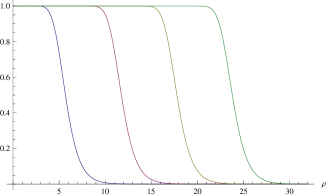
Figure 7: Configurations of the magnetic flux $-\frac{2}{m^{2}}F_{12}=1-e^{-\psi}$ for $\nu=9,36,81,144$ of which radiuses are estimated to be $mR=6,12,18,24$ respectively.

A profile of the domain-wall is almost invariant with various values of $\nu$. For large $\nu$, therefore, a contribution to the total energy $T_{\rm bag}$ form the domain-wall can be negligible.

Since a vortex configuration for large $\nu$ drastically changes around the domain-wall at $r\approx R\gg 1/m$, we expect that the approximation for $r\ll R_{\rm in}$ in Eq.(2.43) is applicable for $r=R-\epsilon<R$ with $\epsilon={\cal O}(1/m)$ as

$${\cal O}(1)\approx\psi(R-\epsilon)\approx-2\nu\log\left(m(R-\epsilon)\right)+2D_{\nu}\approx 2\nu\log\left(\frac{R_{\rm in}}{R}\right),$$ (4.8)

and similarly the asymptotic behavior in Eq.(2.55) is applicable for $r=R+\epsilon$

$${\cal O}(1)\approx\psi(R+\epsilon)\approx C_{\nu}K_{0}(m(R+\epsilon))\approx C_{\nu}\sqrt{\frac{\pi}{2mR}}e^{-mR}.$$ (4.9)

Inserting $R=R_{\rm BPS}=2\sqrt{\nu}/m$, these estimations give large-$\nu$ behaviors of $C_{\nu}$ and $D_{\nu}$ as

$$C_{\nu}\approx{\cal O}(1)\times\nu^{\frac{1}{4}}e^{2\sqrt{\nu}},\quad D_{\nu}\approx\frac{\nu}{2}\left(\log\nu+{\cal O}(1)\right).$$ (4.10)

We also estimate $S_{\nu}$ as

$$S_{\nu}=\frac{m^{2}}{2}\int\frac{d^{2}x}{2\pi}(1-e^{-\psi})^{2} \approx \frac{1}{4\pi}\times\pi(mR)^{2}+\frac{1}{4\pi}\times{\cal O}(1)\times 2\pi mR+{\cal O}(R^{0})$$ (4.11)

$$\approx \nu-\beta\,\sqrt{\nu}+{\cal O}(\nu^{0}).$$

Not that the term proportional to $\sqrt{\nu}$ comes from contribution of surface of the vortex and the coefficient $\beta$ must be positive due to Eq.(2.64). The above estimations for large $\nu$ will become important clues to modify the approximations using the $\nu$-expansion.

4.2 (Global) Padé approximations

Let us assume that we know only a finite series of order $n$,

$$E_{n}[F(\nu)]=\sum_{k=0}^{n}f_{k}\nu^{k},$$ (4.12)

as a part of a certain infinite series $F(\nu)$ and it behaves as almost an alternating series like $F(\nu)=|f_{0}|-|f_{1}|\nu+|f_{2}|\nu^{2}-...$, and it seems to have a small radius of convergence $\nu\approx\nu_{\rm c}$. To get a good approximation for $\nu>\nu_{\rm c}$ with such a series, it is powerful to use the Padé approximation which replace the series by some rational functions, with $n=m+l$,

$$E_{n}[F(\nu)]=P_{(m,l)}[F(\nu)]+{\cal O}(\nu^{m+l+1}).$$ (4.13)

where a Padé approximant of $F(\nu)$ is given by

$$P_{(m,l)}[F(\nu)]=\frac{\displaystyle a_{0}+\sum_{n=1}^{m}a_{n}\nu^{n}}{\displaystyle 1+\sum_{n=1}^{l}b_{n}\nu^{n}},$$ (4.14)

where coefficients of these rational functions are determined so that they satisfies

$$\frac{d^{k}F(\nu)}{d\nu^{k}}\Big{|}_{\nu=0}=\frac{d^{k}}{d\nu^{k}}P_{(m,l)}[F(\nu)]\Big{|}_{\nu=0}\quad{\rm for~{}}k=0,1,\cdots,m+l.$$ (4.15)

Here the two sets $\{a_{n}\}$ and $\{b_{n}\}$ are determined uniquely from the finite set $\{f_{0},f_{2},\cdots,f_{n+m}\}$.

There is arbitrariness in a choice of $(m,l)$ for the order $n$. The approximant $P_{(m,l)}[F(\nu)]$ behaves for large $\nu$ as

$$P_{(m,l)}[F(\nu)]\approx\frac{a_{m}}{b_{l}}\nu^{m-l}.$$ (4.16)

Note that if we fix $p=m-l$ to remove that arbitrariness, then $n$ is restricted so that $n-p=2l$. In the case of $p=1$ for example, we arrange the Padé approximants for all of the order $n$ as

$$P_{(1,0)}[F(\nu)],\quad\sqrt{P_{(2,0)}[F(\nu)^{2}]},\quad P_{(2,1)}[F(\nu)],\quad\sqrt{P_{(4,2)}[F(\nu)^{2}]},\cdots.$$ (4.17)

4.2.1 $\widehat{P}_{n}[S_{\nu}]$

The series expansion for $S_{\nu}$ seems to be almost alternative series, and according to configurations for the finite series $E_{n}[S_{\nu}]$ shown in the left panel of Fig.4 we guess that the radius of convergence is around $|\nu|\approx 0.5$ which implies, for instance, that the function $S_{\nu}$ has a singularity at $\nu\approx-0.5$. The Padé approximation can avoid such a singularity and enlarge the radius of convergence. Let us take the following rational functions $P_{n}[S_{\nu}]$ with respect to $\nu$, as Padé approximants of the order $n$ for $S_{\nu}$,

$$P_{2}[S_{\nu}] = P_{(2,1)}[S_{\nu}]=\frac{\nu^{2}}{1+1.5626\nu},$$

$$P_{3}[S_{\nu}] = P_{(3,1)}[S_{\nu}]=\frac{\nu^{2}+0.189609\nu^{3}}{1+1.75221\nu},$$

$$P_{4}[S_{\nu}] = P_{(3,2)}[S_{\nu}]=\frac{\nu^{2}+1.05188\nu^{3}}{1+2.61449\nu+1.34739\nu^{2}},$$

$$P_{5}[S_{\nu}] = P_{(4,2)}[S_{\nu}]=\frac{\nu^{2}+1.34536\nu^{3}+0.0556454\nu^{4}}{1+2.90796\nu+1.86162\nu^{2}},$$

$$P_{6}[S_{\nu}] = P_{(4,3)}[S_{\nu}]=\frac{\nu^{2}+1.94979\nu^{3}+0.69144\nu^{4}}{1+3.5124\nu+3.44191\nu^{2}+0.814411\nu^{3}}.$$ (4.18)

Here we have fixed arbitrariness on choice of the Padé approximants $P_{(m,n)}[S_{\nu}]$ so that all coefficients of the above are positive. As a result poles and zeros of these functions turn out to sit only on the negative real axis of $\nu$ as shown in Fig.8 and the rational functions $P_{n}[S_{\nu}]$ have poles around $\nu\approx-0.5$ in common.

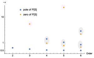
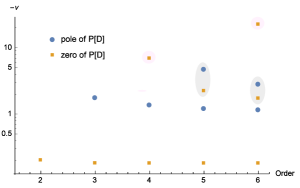
Figure 8: Poles and Zeros for $P_{n}[S_{\nu}]/\nu^{2}$ in the left panel, and for $P_{n}[D_{\nu}]/\nu$ in right panel. We observe common poles $\nu\approx-0.5$ for $P_{n}[S_{\nu}]$ and $\nu\approx-1$ for $P_{n}[D]$ and a common zero $\nu\approx-0.2$ for $P_{n}[D]$. A pair of a pole and an adjacent zero do not change a large-$\nu$ behavior remarkably.

Actually these functions give good approximations in a wider range of $\nu$ as shown in Fig.9.

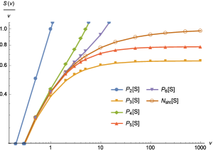
Figure 9: Profiles of $P_{n}[S_{\nu}]$ in the left panel and their errors from numerical data of $S_{\nu}$ calculated by the shooting method, $|P_{n}[S_{\nu}]/N_{\rm sht}[S_{\nu}]-1|$ in the right panel.

Note that these rational functions behave as

$$P_{2n}[S_{\nu}]={\cal O}(\nu),\quad P_{2n+1}[S_{\nu}]={\cal O}(\nu^{2}),\quad{\rm for~{}large~{}}\nu,$$ (4.19)

and $P_{2n}[S_{\nu}]$ give comparatively good approximations even for large $\nu$. This property can be understood if we take account of the behavior of $S_{\nu}$ for large $\nu$ shown in Eq.(4.11). Extra zeros $\nu\approx-5.27$ of $P_{3}[S_{\nu}]$ and $\nu\approx-23.4$ of $P_{5}[S_{\nu}]$ shown in Fig.8 can be regarded as disturbances for large-$\nu$ behaviors.

Let us consider the large-$\nu$ behavior more seriously. The large-$\nu$ behavior in Eq.(4.11) does not always mean that the function $S_{\nu}$ has a branch cut. For an example, a function $\sqrt{\nu}\tanh(\sqrt{\nu})$ has no branch cut anywhere although it behaves $\sqrt{\nu}$ for large $\nu\in\mathbb{R}_{>0}$. Here, we just assume existence of a branch cut. For instance, a function

$$\widehat{P}_{1}[S_{\nu}]=\nu-\nu\sqrt{\frac{1}{1+2\nu}}$$ (4.20)

has a branch point at $\nu=-1/2$ and desirable behaviors as

$$\widehat{P}_{1}[S_{\nu}]=\left\{\begin{array}[]{cc}\nu^{2}+{\cal O}(\nu^{3})&{\rm for~{}}\nu\ll 1/2\\ \nu-\sqrt{\frac{\nu}{2}}+{\cal O}({\sqrt{\nu}}^{-1})&{\rm for~{}}\nu\gg 1/2\end{array}\right.\,,$$ (4.23)

and consequently it works as a quite good approximation for the full range of $\nu$ as shown in Fig.4. The Padé approximation taking account of informations for large $\nu$ is called the global Padé approximation [24]. Note that an expansion of the following quantity is also alternative series due to the singularity,

$$\left(1-\frac{S_{\nu}}{\nu}\right)^{2} = 1-2\nu+4.12521\nu^{2}-8.60125\nu^{3}$$ (4.24)

$$\quad+18.0239\nu^{4}-37.857\nu^{5}+79.5748\nu^{6}+{\cal O}(\nu^{7}),$$

Let us apply the Padé approximation to the above series or its squared quantity. According to Eq.(4.11), the above quantity behaves as ${\cal O}(\nu^{-1})$ for large $\nu$ and this property fixes the arbitrariness of Padé approximants completely. Addition to $\widehat{P}_{1}[S_{\nu}]$ in the above, then, we obtain the following functions as the global Padé approximants of $S_{\nu}$,

$$\widehat{P}_{2}[S_{\nu}] = \nu-\nu\sqrt[4]{\frac{1}{1+4\nu+3.74958\nu^{2}}},$$

$$\widehat{P}_{3}[S_{\nu}] = \nu-\nu\sqrt{\frac{1+0.80192\nu}{1+2.80192\nu+1.47863\nu^{2}}},$$

$$\widehat{P}_{4}[S_{\nu}] = \nu-\nu\sqrt[4]{\frac{1+0.697034\nu}{1+4.69703\nu+6.53772\nu^{2}+2.31356\nu^{3}}},$$

$$\widehat{P}_{5}[S_{\nu}] = \nu-\nu\sqrt{\frac{1+1.11774\nu+0.064997\nu^{2}}{1+3.11774\nu+2.17527\nu^{2}+0.0904502\nu^{3}}},$$

$$\widehat{P}_{6}[S_{\nu}] = \nu-\nu\sqrt[4]{\frac{1+1.81492\nu+0.525555\nu^{2}}{1+5.81492\nu+11.5348\nu^{2}+8.60739\nu^{3}+1.63522\nu^{4}}},$$

which behave for large $\nu$ as

$$\widehat{P}_{n}[S_{\nu}]=\nu-\beta_{n}\sqrt{\nu}+{\cal O}\left(\frac{1}{\sqrt{\nu}}\right),$$ (4.26)

with coefficients for $n=1,2,\cdots$,

$$\{\beta_{n}\}=\{0.707107,0.718628,0.736437,0.740872,0.847699,0.75294,\cdots\}.\qquad$$ (4.27)

At this stage we do not know whether $\beta_{n}$ converges to a true value of $\beta$. As we see in Fig.10, the global Padé approximation works well and $\widehat{P}_{6}[S_{\nu}]$ has a quite small errors less than $10^{-3}$ in the full range of $\nu$.

Figure 10: Errors $|\widehat{P}_{n}[S_{\nu}]/N_{\rm sht}[S_{\nu}]-1|$ of Global Padé approximations $\hat{P}_{n}[S_{\nu}]$ for $S_{\nu}$. Distortion of a profile with $n=6$, at $\nu=1/20$ is consistent to errors of $N_{\rm sht}[S_{\nu}]$ itself shown in Fig.5.

Even for small $\nu$, the global Padé approximants $\widehat{P}_{n}[S_{\nu}]$ give the best result as shown in Fig.11 and the best approximant $\widehat{P}_{6}[S_{\nu}]$ gives

$$\widehat{P}_{6}[S_{1}] = 0.4153585\dots,\qquad\left|\widehat{P}_{6}[S_{1}]/N_{\rm sht}[S_{1}]-1\right|\approx 1.3\times 10^{-5}.$$ (4.28)

Figure 11: Errors of $S_{1}$ in the left panel, and $S_{5}$ in the right panel.

These are the satisfactory values enough as results with the small winding-number expansion.

4.2.2 $\widehat{P}_{n}[D_{\nu}]$

The $\nu$-expansion of $D_{\nu}$ given in Eq.(3.18) also seems to be almost an alternating series and have a finite radius of convergence as shown in Fig.2. Hence let us consider Padé approximations of $E_{n}[D_{\nu}]$. We can fix arbitrariness of the Pad’e approximation by requiring that all coefficients are positive as,

$$P_{3}[D_{\nu}] = \frac{0.115932\nu+0.652038\nu^{2}}{1+0.569826\nu},\quad$$

$$P_{4}[D_{\nu}] = \frac{0.115932\nu+0.67104\nu^{2}+0.0960493\nu^{3}}{1+0.733739\nu},\quad$$

$$P_{5}[D_{\nu}] = \frac{0.115932\nu+0.706900\nu^{2}+0.297736\nu^{3}}{1+1.04306\nu+0.176257\nu^{2}}$$

$$P_{6}[D_{\nu}] = \frac{0.115932\nu+0.728018\nu^{2}+0.419974\nu^{3}+0.0174966\nu^{4}}{1+1.22522\nu+0.309917\nu^{2}},$$ (4.30)

which have a pole $\nu\approx-1$ in common as seen in Fig.8. As shown in Fig.12 $P_{n}[D_{\nu}]$ give comparatively good approximations.

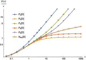
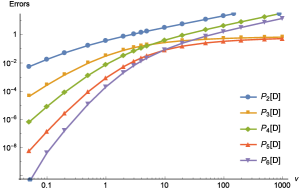
Figure 12: Profiles and errors of $P_{n}[D_{\nu}]$

To get better approximations, let us apply the Padé approximation not to $D_{\nu}$ it self, but to $\exp(2nD_{\nu}/\nu)$ with $n=1,2,4$, then we obtain

$$\widehat{P}_{2}[D_{\nu}] = \frac{\nu}{2}\log\left(\frac{0.853276+\nu}{0.676695}\right),$$

$$\widehat{P}_{3}[D_{\nu}] = \frac{\nu}{2}\log\left(\frac{\sqrt{0.708551+1.66078\nu+\nu^{2}}}{0.667557}\right),$$

$$\widehat{P}_{4}[D_{\nu}] = \frac{\nu}{2}\log\left(\frac{0.654559+1.60982\nu+\nu^{2}}{0.519101+0.668311\nu}\right),$$

$$\widehat{P}_{5}[D_{\nu}] = \frac{\nu}{2}\log\left(\frac{\sqrt[4]{0.511978+2.40006\nu+4.25790\nu^{2}+3.38280\nu^{3}+\nu^{4}}}{0.670835}\right),$$

$$\widehat{P}_{6}[D_{\nu}] = \frac{\nu}{2}\log\left(\frac{2.17939+5.34930\nu+4.17049\nu^{2}+\nu^{3}}{1.72838+2.21671\nu+0.676831\nu^{2}}\right).$$ (4.31)

These functions have the same behavior for large $\nu$ as Eq.(4.10),

$$\widehat{P}_{n}[D_{\nu}]\approx\frac{\nu}{2}\log\left(\frac{\nu}{\alpha_{n}}\right),\quad\alpha_{n}<e/4\approx 0.679570.$$ (4.32)

Hence, as shown in Fig.13 and Fig.14, these give quite good approximations and errors of $\widehat{P}_{6}[D_{\nu}]$ are less than $10^{-3}$ in the full range of $\nu$.

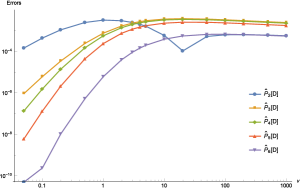
Figure 13: Errors in global Padé approximations for $D_{\nu}$.

The best approximant we obtained gives

$$\widehat{P}_{6}[D_{1}]=0.5053639\dots,\qquad|\widehat{P}_{6}[D_{1}]/N_{\rm sht}[D_{1}]-1|\approx 6.1\times 10^{-6},$$

$$2\exp(-2\widehat{P}_{6}[D_{1}])=0.727908\dots,$$ (4.33)

which reproduces the numerical result presented by de Vega and Schaposnik. This value with the similar accuracy was also obtained analytically in Ref.[25]. @

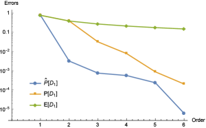
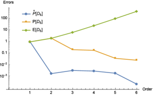
Figure 14: Errors of $D_{1}$ in the left panel, and $D_{5}$ in the right panel.

4.2.3 $\widehat{P}_{n}[C_{\nu}]$

The $\nu$-expansion of $C_{\nu}$ in Eq.(3.13) gives a quite good approximation for $C_{\nu}$, at least for $\nu=1$ and we do not know whether the radius of convergence is larger than one or not. In this stage, therefore, it is not useful to apply the (ordinary) Padé approximation to $E_{n}[C_{\nu}]$. Once we take account of the large-$\nu$ behavior of $C_{\nu}$ given in Eq.(4.10), however, we notice that there exists a singularity at the infinity and we have to remove this at the first stage.

Let us consider the following function

$${\widetilde{C}}_{\nu}\equiv\frac{\sqrt{\nu}}{2}\sinh(2\sqrt{\nu})$$ (4.34)

which has an infinite number of zeros on a negative real axis of $\nu$ and regular everywhere except for an essential singularity at the infinity. The nearest next zero to the origin is $\nu=-\pi^{2}/4\approx-2.47$. It is, therefore, natural to assume that a quantity $F_{\nu}\equiv(C_{\nu}/{\widetilde{C}}_{\nu})^{4}$ has an infinite number of poles (and zeros) on the negative real axis of $\nu$. Actually we find that an expansion of $F_{\nu}$ gives an almost alternative series as,

$$F_{\nu}=\left(\frac{C_{\nu}}{{\widetilde{C}}_{\nu}}\right)^{4} = 1-0.248268\nu+0.020833\nu^{2}+0.034017\nu^{3}$$ (4.35)

$$\quad-0.0342630\nu^{4}+0.0226871\nu^{5}+{\cal O}(\nu^{6}).$$

According to Eq.(4.10), $F_{\nu}$ must behave for large $\nu$ as

$$F_{\nu}=\frac{{\rm const.}}{\nu}+{\cal O}(\nu^{-2}),$$ (4.36)

which means that we removed the singularity at the infinity in success. Next, let us apply the Padé approximation to the series in Eq.(4.35) or its squared quantity, satisfying the property Eq.(4.36). We obtain,

$$\widehat{P}_{1}[C_{\nu}] = {\widetilde{C}}_{\nu},\quad\widehat{P}_{2}[C_{\nu}]={\widetilde{C}}_{\nu}\sqrt[4]{\frac{1}{1+0.248268\nu}},$$

$$\widehat{P}_{3}[C_{\nu}] = {\widetilde{C}}_{\nu}\sqrt[8]{\frac{1}{1+0.496535\nu+0.143244\nu^{2}}},$$

$$\widehat{P}_{4}[C_{\nu}] = {\widetilde{C}}_{\nu}\sqrt[4]{\frac{1+0.712165\nu}{1+0.960432\nu+0.217611\nu^{2}}},$$

$$\widehat{P}_{5}[C_{\nu}] = {\widetilde{C}}_{\nu}\sqrt[8]{\frac{1+0.600743\nu}{1+1.09728\nu+0.441534\nu^{2}+0.0481954\nu^{3}}},$$

$$\widehat{P}_{6}[C_{\nu}] = {\widetilde{C}}_{\nu}\sqrt[4]{\frac{1+0.709639\nu+0.0702914\nu^{2}}{1+0.957906\nu+0.287275\nu^{2}+0.017348\nu^{3}}}.$$ (4.38)

where we added $\widehat{P}_{1}[C_{\nu}]$ to the above although it does not satisfy Eq.(4.36). We observe the large-$\nu$ behaviors of them except for $\widehat{P}_{1}[C_{\nu}]$ as

$$\widehat{P}_{n}[C_{n}]\approx\omega_{n}\sqrt[4]{\nu}e^{2\sqrt{\nu}}$$ (4.39)

with coefficients

$$\{\omega_{2},\omega_{3},\cdots\}=\{{0.354169},{0.318735},{0.336252},{0.342689},{0.354693},\cdots\}.$$ (4.40)

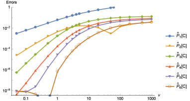
Figure 15: Errors of global Padé approximants $\widehat{P}_{n}[C_{\nu}]$ for $C_{\nu}$.

In Fig.15, we observe that these functions give nice approximants in the full range of $\nu$ and modify $E_{n}[C_{\nu}]$ as shown in Fig.6. Resultantly, even for $C_{1}$, we succeeded in reproducing the numerical result $C_{1}=1.7079$ given by de Vega and Schaposnik as

$$\widehat{P}_{6}[C_{1}]=1.7078629\dots,\quad\left|\frac{\widehat{P}_{6}[C_{1}]}{N_{\rm sht}[C_{1}]}-1\right|=7.2\times 10^{-7}.$$ (4.41)

5 Summary and Discussion

We considered the small winding-number expansion (the $\nu$-expansion) of the solution of the Taubes equation by extending the winding number, which is a topological quantum number, to be a real number larger than $-1$. We confirmed that the $\nu$-expansion is useful to give good approximations of axially-symmetric vortex solutions in most of the range allowed for the winding number. Finally we found that for the scalar charge $C_{1}$ the best approximate value in terms of the $\nu$-expansion with the help of the Padé approximation is $\widehat{P}_{6}[C_{1}]=1.7078629\dots$, which coincides with a value $N_{\rm sht}[C_{1}]=1.707864175$, obtained numerically by the shooting method. We judged that the result given by de Vega and Schaposnik is correct, and Tong’s conjecture giving $C_{1}=8^{\frac{1}{4}}\approx 1.68$ from superstring theory perspective is incorrect as a vortex solution in the Abelian-Higgs model. Their numerical similarity might suggest a certain universality.

The Abelian-Higgs model of critical coupling is just the simplest toy model to test and establish usefulness of the $\nu$-expansion. The idea of the $\nu$-expansion is rather simple and more straightforward than the strategy taken by de Vega & Schaposnik. As for BPS states of vortices in further complicated systems like non-Abelian gauge-Higgs models or of separated (parallel) multi-vortices, therefore, it is expected that the $\nu$-expansion can be straightforwardly applied to their analytical approximations. Since it is difficult to apply the shooting method to such complicated systems, we guess that the role of the $\nu$-expansion will become more important there. The $\nu$-expansion is also expected to be powerful to analyze dependence on dimensionless parameters of solutions, like dependence on the number $N$ and a ratio of two gauge couplings of $U(N)=[U(1)\times SU(N)]/\mathbb{Z}_{N}$ for an $U(N)$ vortex.

We expect that the $\nu$-expansion can be applied to systems of non-critical coupling, although it might not be a straightforward extension. Our final goal is to establish a systematic tool to study the dynamics of vortices quantitatively without taking the critical coupling limit. Since in the $\nu$-expansion vortices are treated as singular particles (strings) in a three(four)-dimensional spacetime, it will become possible to treat vortices of arbitrary shapes and discuss their dynamics analytically and quantitatively if we can consider such an extended $\nu$-expansion.

Appendix A Inequalities

A.1 Uniqueness of the solution

Let us show the uniqueness of the solution $f(\vec{x})$ of the following $d$-dimensional partial differential equation defined by a strictly increasing function ${\cal W}(f)$ with respect to $f$ and a source term $J$ as

$$-{\partial}_{i}^{2}f(\vec{x})+{\cal W}(f(\vec{x}))=J(\vec{x}),$$ (A.1)

where we require that $f(\vec{x})$ vanishes at the spatial infinity. Note that if there exists a region $\Sigma_{f}$ with its boundary ${\partial}\Sigma_{f}$ for a certain scalar function $f(\vec{x})$ so that $f(\vec{x})$ satisfies

$$f(\vec{x})<0~{}{\rm for~{}}\vec{x}\in\Sigma,\qquad f(\vec{x})=0~{}{\rm for~{}}\vec{x}\in\partial\Sigma,$$ (A.2)

which gives $\vec{n}\cdot\vec{\partial}f(\vec{x})\geq 0$ with a normal vector $\vec{n}$ of ${\partial}\Sigma$ and then Stokes’ theorem tells us the following inequality

$$\int_{\Sigma_{f}}d^{d}x{\partial}^{2}_{i}f(\vec{x})=\int_{{\partial}\Sigma_{f}}d\vec{S}\cdot\vec{\partial}f(\vec{x})\geq 0.$$ (A.3)

If we assume that there exist different two solutions $f_{1}(\vec{x}),f_{2}(\vec{x})$ for Eq.(A.1), then there exists the region $\Sigma_{\delta f}$ for a difference $\delta f=f_{1}-f_{2}$(or $f_{2}-f_{1}$) and we can derive inconsistency as,

$$0\leq\int_{\Sigma_{\delta f}}d^{d}x{\partial}_{i}^{2}\delta f(\vec{x})=\int_{\Sigma_{\delta f}}d^{d}x\left\{{\cal W}(f_{1}(\vec{x}))-{\cal W}(f_{2}(\vec{x}))\right\}<0.$$ (A.4)

Therefore, if there exist a solution of Eq.(A.1), then it must be unique.

Furthermore, let us consider a solution $f(\vec{x})$ with ${\cal W}(0)=0$ and $J(\vec{x})\geq 0$,

$$-{\partial}_{i}^{2}f(\vec{x})+{\cal W}(f(\vec{x}))\geq 0.$$ (A.5)

If there exist a region $\Sigma_{f}$ for this function $f$ where ${\cal W}(f)<0$, then we find inconsistency again

$$0\leq\int_{\Sigma_{f}}d^{d}x{\partial}^{2}_{i}f(\vec{x})\leq\int_{\Sigma_{f}}d^{d}x{\cal W}(f(\vec{x}))<0.$$ (A.6)

Such a solution $f(\vec{x})$ must be, therefore, positive semidefinite everywhere.

A.2 Sequence of sets of upper and lower bounds

Here let us modify the inequality Eq.(2.37) for $\nu>0$.

$${\cal I}_{0}:\infty>\psi>0,\quad 0>P\equiv r\frac{{\partial}\psi}{{\partial}r}>-2\nu,$$ (A.7)

to obtain a stronger set of upper and lower bounds of them.

By integrating Taubes equation and $P=r\psi^{\prime}$, we find relations between $P$ and $\psi$ using integrals as, with $Y=(r/R_{\rm in})^{2\nu}$ and setting $m=1$,

$$\psi = \Psi[P]\equiv\lim_{\epsilon\to 0}\left\{-2\nu\log\left(\frac{\epsilon}{R_{\rm in}}\right)+\int_{\epsilon}^{r}\frac{ds}{s}P(s)\right\}=-\log Y+\int_{0}^{r}\frac{ds}{s}(P(s)+2\nu),$$

$$P = {\cal P}[\psi]\equiv-2\nu+\int_{0}^{r}ds\,s\left(1-e^{-\psi(s)}\right).$$ (A.8)

Let us assume that the following set of inequalities ${\cal I}_{n}$

$${\cal I}_{n}:f_{n}^{\rm M}>\psi>f_{n}^{\rm m},\quad g_{n}^{\rm M}>P>g_{n}^{\rm m},\qquad{\rm for~{}all~{}}r\in\mathbb{R}_{>0}.$$ (A.9)

with some given functions $f_{n}^{\rm M,m},g_{n}^{\rm M,m}$ satisfying

$$\cdots\geq f_{n-1}^{\rm M}\geq f_{n}^{\rm M}>f_{n}^{\rm m}\geq f_{n-1}^{\rm m}\geq\cdots\geq f_{0}^{\rm m}=0,$$

$$0=g_{0}^{\rm M}\geq\cdots\geq g_{n-1}^{\rm M}\geq g_{n}^{\rm M}>g_{n}^{\rm m}\geq g_{n-1}^{\rm m}\geq\cdots\geq g_{0}^{\rm m}=-2\nu.$$ (A.10)

Using these inequalities, we can construct an another set of inequalities as

$$\Psi[g_{n}^{\rm M}]>\psi>\Psi[g_{n}^{\rm m}],\quad{\cal P}[f_{n}^{\rm M}]>P>{\cal P}[f_{n}^{\rm m}].$$ (A.11)

Therefore we obtain a set of stronger lower and upper bounds as ${\cal I}_{n+1}$ by

$$g_{n+1}^{\rm M}={\rm min}\left[g_{n}^{\rm M},{\cal P}[f_{n}^{\rm M}]\right],\quad g_{n+1}^{\rm m}={\rm max}\left[g_{n}^{\rm m},{\cal P}[f_{n}^{\rm m}]\right],$$

$$f_{n+1}^{\rm M}={\rm min}\left[f_{n}^{\rm M},\Psi[g_{n}^{\rm M}]\right],\quad f_{n+1}^{\rm m}={\rm max}\left[f_{n}^{\rm m},\Psi[g_{n}^{\rm m}]\right].$$ (A.12)

Consistency of these inequalities requires that $g_{n+1}^{\rm M}>g_{n+1}^{\rm m}$ and $f_{n+1}^{\rm M}>f_{n+1}^{\rm m}$ which reduce to, non-trivial inequalities

$$0=g_{0}^{\rm M}>{\cal P}[f_{n}^{\rm m}],\quad\Psi[g_{n}^{\rm M}]>f_{0}^{\rm m}=0.$$ (A.13)

This couple of inequalities turns out to give lower and upper bounds for $R_{\rm in}$ as follows.

The initial set of inequalities ${\cal I}_{0}$ gives

$${\cal I}_{1} : \infty>\psi>{\rm max}[0,-\log Y],\quad\min\left[\frac{r^{2}}{2}-2\nu,0\right]>P>-2\nu,$$ (A.14)

and therefore we find the followings are required

$$0>{\max}\,{\cal P}[f_{1}^{\rm m}]\quad \to \quad 2\nu>\int_{0}^{R_{\rm in}}drr\left(1-\left(\frac{r}{R_{\rm in}}\right)^{2\nu}\right)=\frac{\nu R_{\rm in}^{2}}{2(1+\nu)},$$

$$0<\min\Psi[g_{1}^{\rm M}]\quad \to \quad 0<\frac{r^{2}}{4}-\log Y\Big{|}_{r=2\sqrt{\nu}}=\nu\log\left(\frac{R_{\rm in}^{2}e}{4\nu}\right),$$ (A.15)

and that is, $R_{\rm in}$ must satisfy

$$2\sqrt{\nu+1}>R_{\rm in}>2\sqrt{\frac{\nu}{e}},$$ (A.16)

otherwise a function $\psi$ can not satisfy the set of inequalities ${\cal I}_{0}$ and thus blows up at large $r$. With $R_{\rm in}$ satisfying the above set of inequalities, the next set of inequalities ${\cal I}_{2}$ can be consistently obtained as

$${\cal I}_{2} : {\rm max}[0,-\log Y]<\psi<\left\{\begin{array}[]{cc}\frac{r^{2}}{4}-\log Y&{\rm for~{}}r\leq 2\sqrt{\nu}\\ \nu\log\left(\frac{R_{\rm in}^{2}e}{4\nu}\right)&{\rm for~{}}r>2\sqrt{\nu}\end{array}\right.\,,$$ (A.22)

$$\min\left[\frac{r^{2}}{2}-2\nu,0\right]>P>\left\{\begin{array}[]{cc}-2\nu+\frac{r^{2}}{2}\left(1-\frac{Y}{1+\nu}\right)&{\rm for~{}}r\leq R_{\rm in}\\ -2\nu+\frac{\nu R_{\rm in}^{2}}{2(1+\nu)}&{\rm for~{}}r>R_{\rm in}\end{array}\right.\,.\qquad\quad$$

In principle, you can calculate ${\cal I}_{3},{\cal I}_{4},\dots,$ sequentially as you like.

Appendix B Some Integrals

Since the modified Bessel function of the second kind is a two dimensional Green’s function, we can find the following relations

$$\int d^{2}xK_{0}(m|\vec{x}-\vec{x}_{1}|)K_{0}(m|\vec{x}-\vec{x}_{2}|)$$ (B.1)

$$= \frac{2\pi}{-\partial^{2}+m^{2}}K_{0}(m|\vec{x}_{1}-\vec{x}_{2}|)$$

$$= \left(\frac{2\pi}{-\partial^{2}+m^{2}}\right)^{2}\delta^{2}(\vec{x}_{1}-\vec{x}_{2})=-\frac{\partial}{\partial m^{2}}\frac{4\pi^{2}}{-\partial^{2}+m^{2}}\delta^{2}(\vec{x}_{1}-\vec{x}_{2})$$

$$= -2\pi\frac{\partial}{\partial m^{2}}K_{0}(m|\vec{x}_{1}-\vec{x}_{2}|)=\frac{\pi}{m}|\vec{x}_{1}-\vec{x}_{2}|K_{1}(m|\vec{x}_{1}-\vec{x}_{2}|)$$

By using the integral formulas

$$K_{0}(x)=\int_{0}^{\infty}\frac{dt}{2t}e^{-\frac{x}{2}\left(t+\frac{1}{t}\right)},\quad I_{0}(x)=\int_{0}^{2\pi}\frac{d\theta}{2\pi}e^{x\cos\theta},$$ (B.2)

one can calculate the following definite integrals,

$$= \int_{0}^{\infty}drrI_{0}(r)K_{0}(r)^{3}=\int\frac{d^{2}x}{2\pi}e^{x_{1}}K_{0}(|\vec{x}|)^{3}$$ (B.3)

$$= \int\frac{d^{2}x}{2\pi}\frac{dt_{1}dt_{2}dt_{3}}{8t_{1}t_{2}t_{3}}e^{x_{1}-(t_{1}+t_{2}+t_{3})-\frac{(x_{1}^{2}+x_{2}^{2})}{4}\left(\frac{1}{t_{1}}+\frac{1}{t_{2}}+\frac{1}{t_{3}}\right)}$$

$$= \int_{0}^{\infty}\frac{dt_{1}dt_{2}dt_{3}}{4t_{1}t_{2}t_{3}\left(\frac{1}{t_{1}}+\frac{1}{t_{2}}+\frac{1}{t_{3}}\right)}e^{-(t_{1}+t_{2}+t_{3})+\left(\frac{1}{t_{1}}+\frac{1}{t_{2}}+\frac{1}{t_{3}}\right)^{-1}}$$

$$= \frac{1}{4}\int_{0}^{\infty}\frac{du_{1}du_{2}}{(1+u_{1})(1+u_{2})(u_{1}+u_{2})}=\frac{\pi^{2}}{16}$$

with $t_{1}=su_{1},t_{2}=su_{2},t_{3}=s$,

$$= \int\frac{d^{2}xd^{2}y}{4\pi^{2}}I_{0}(|\vec{x}|)K_{0}(|\vec{x}|)K_{0}(|\vec{x}-\vec{y}|)K_{0}(|\vec{y}|)^{2}$$ (B.4)

$$= \frac{1}{4}\int_{0}^{\infty}\frac{dt_{1}dt_{2}dt_{3}dt_{4}}{t_{1}t_{2}+(t_{1}+t_{2})(t_{3}+t_{4})}e^{-(t_{1}+t_{2}+t_{3}+t_{4})+\left(\frac{1}{t_{4}}+\frac{1}{t_{3}+(1/t_{1}+1/t_{2})^{-1}}\right)^{-1}}$$

$$= \frac{11\pi^{2}}{432},$$

$$= \int_{0}^{\infty}drrK_{0}(r)^{3}=\int_{0}^{\infty}\frac{dt_{1}dt_{2}dt_{3}}{4t_{1}t_{2}t_{3}\left(\frac{1}{t_{1}}+\frac{1}{t_{2}}+\frac{1}{t_{3}}\right)}e^{-(t_{1}+t_{2}+t_{3})}$$ (B.5)

$$= \frac{1}{4}\int_{0}^{\infty}\frac{du_{1}du_{2}}{(1+u_{1}+u_{2})(u_{1}+u_{2}+u_{1}u_{2})}$$

$$= \frac{1}{36}\left\{\psi^{(1)}\left(\frac{1}{3}\right)+\psi^{(1)}\left(\frac{1}{6}\right)-\frac{8\pi^{2}}{3}\right\}\approx 0.585977$$

where $\psi^{(1)}(x)=d^{2}\log\Gamma(x)/dx^{2}$ is the digamma function, and

$${\begin{minipage}[h]{52.03227pt} \includegraphics[width=433.62pt,keepaspectratio={true}]{v4.eps} \end{minipage}}=\int_{0}^{\infty}drrK_{0}(r)^{4}=\frac{7}{8}\zeta(3)\approx 1.051800.$$ (B.6)

References

- [1] M. F. Atiyah, N. J. Hitchin, V. G. Drinfeld and Y. .I. Manin, “Construction of Instantons,” Phys. Lett. A 65, 185 (1978).
- [2] V. L. Ginzburg and L. D. Landau, “On the Theory of superconductivity,” Zh. Eksp. Teor. Fiz. 20 (1950) 1064.
- [3] A. A. Abrikosov, “On the Magnetic properties of superconductors of the second group,” Sov. Phys. JETP 5 (1957) 1174 [Zh. Eksp. Teor. Fiz. 32 (1957) 1442].
- [4] H. B. Nielsen and P. Olesen, “VORTEX-LINE MODELS FOR DUAL STRINGS,” Nucl. Phys. B 61, 45 (1973).
- [5] H. J. de Vega and F. A. Schaposnik, “A Classical Vortex Solution Of The Abelian Higgs Model,” Phys. Rev. D 14, 1100 (1976).
- [6] L. Jacobs and C. Rebbi, “Interaction Energy Of Superconducting Vortices,” Phys. Rev. B 19, 4486 (1979).
- [7] D. Cabra, C. von Reichenbach, F. A. Schaposnik and M. Trobo, “Topologically nontrivial sectors in the Abelian Higgs model with massless fermions,” Phys. Rev. D 44, 3293 (1991).
- [8] A. Vilenkin and E. P. S. Shellard, “Cosmic strings and other topological defects ,” Cambridge, UK: Univ. Pr. (1994) 537 p
- [9] N. S. Manton and P. Sutcliffe, “Topological solitons,” Cambridge, UK: Univ. Pr. (2004) 493 p
- [10] J. M. Speight, “Static intervortex forces,” Phys. Rev. D 55, 3830 (1997) [arXiv:hep-th/9603155].
- [11] D. Tong, “NS5-branes, T-duality and worldsheet instantons,” JHEP 0207, 013 (2002) [arXiv:hep-th/0204186].
- [12] N. S. Manton and J. M. Speight, “Asymptotic interactions of critically coupled vortices,” Commun. Math. Phys. 236, 535 (2003) [arXiv:hep-th/0205307].
- [13] A. Gonzalez-Arroyo and A. Ramos, “Expansion for the solutions of the Bogomolny equations on the torus,” JHEP 0407, 008 (2004) [arXiv:hep-th/0404022].
- [14] C. H. Taubes, “Arbitrary N-Vortex Solutions to the First Order Landau-Ginzburg Equations,” Commun. Math. Phys. 72 (1980) 277.
- [15] M. Eto, T. Fujimori, T. Nagashima, M. Nitta, K. Ohashi and N. Sakai, “Multiple Layer Structure of Non-Abelian Vortex,” Phys. Lett. B 678, 254 (2009) [arXiv:0903.1518 [hep-th]].
- [16] H. Y. Chen and N. S. Manton, “The Kahler potential of Abelian Higgs vortices,” J. Math. Phys. 46 (2005) 052305 [hep-th/0407011].
- [17] T. M. Samols, “Vortex scattering,” Commun. Math. Phys. 145 (1992) 149.
- [18] N. S. Manton and S. M. Nasir, “Conservation laws in a first order dynamical system of vortices,” Nonlinearity 12 (1999) 851 [hep-th/9809071].
- [19] M. Eto, T. Fujimori, M. Nitta, K. Ohashi and N. Sakai, “Higher Derivative Corrections to Non-Abelian Vortex Effective Theory,” Prog. Theor. Phys. 128 (2012) 67 [arXiv:1204.0773 [hep-th]].
- [20] S. B. Bradlow, “Vortices in holomorphic line bundles over closed Kahler manifolds,” Commun. Math. Phys. 135 (1990) 1.
- [21] S. Bolognesi, “Domain walls and flux tubes,” Nucl. Phys. B 730 (2005) 127 [hep-th/0507273].
- [22] S. Bolognesi, “Large N, Z(N) strings and bag models,” Nucl. Phys. B 730 (2005) 150 [hep-th/0507286].
- [23] S. Bolognesi, C. Chatterjee, S. B. Gudnason and K. Konishi, “Vortex zero modes, large flux limit and Ambjorn-Nielsen-Olesen magnetic instabilities,” JHEP 1410 (2014) 101 [arXiv:1408.1572 [hep-th]].
- [24] S. Winitzki, “Uniform approximations for transcendental functions,” in Computational Science and Its Applications–ICCSA, vol. 2667 of Lecture Notes in Computer Science, pp. 780-789, Springer, Berlin, Germany, 2003.
- [25] G. S. Lozano, E. F. Moreno and F. A. Schaposnik, “Nielsen-Olesen vortices in noncommutative space,” Phys. Lett. B 504 (2001) 117 [hep-th/0011205].