A Cut Discontinuous Galerkin Method for the Laplace-Beltrami Operator

Abstract.

We develop a discontinuous cut finite element method (CutFEM) for the Laplace-Beltrami operator on a hypersurface embedded in $\mathbb{R}^{d}$. The method is constructed by using a discontinuous piecewise linear finite element space defined on a background mesh in $\mathbb{R}^{d}$. The surface is approximated by a continuous piecewise linear surface that cuts through the background mesh in an arbitrary fashion. Then a discontinuous Galerkin method is formulated on the discrete surface and in order to obtain coercivity, certain stabilization terms are added on the faces between neighboring elements that provide control of the discontinuity as well as the jump in the gradient. We derive optimal a priori error and condition number estimates which are independent of the positioning of the surface in the background mesh. Finally, we present numerical examples confirming our theoretical results.

KEY WORDS. surface PDE, Laplace-Beltrami, discontinuous Galerkin, cut finite element method

1. Introduction

1.1. Background

Recently there has been a rapid development of so-called cut finite element methods (CutFEM), which provide a technology for discretization of both the geometry of the computational domain and the partial differential equations (PDE) which we seek to solve. The basic idea in CutFEM is to represent the geometry of the domain on a fixed background mesh which is also used to construct the finite element space. The geometric representation of surfaces consists of elementwise smooth surfaces that are allowed to cut through the background mesh in an arbitrary fashion. The active background mesh then consists of all elements that are cut by the domain and the finite element space used in the computation is the restriction to the active mesh. The variational formulation of the PDE is defined on the cut elements. Boundary and interface conditions are enforced weakly. In order to obtain a stable method, independent of the position of the geometry in the background mesh, and to handle the cut elements in the analysis, certain stabilization terms are added that provide control of the local variation of the discrete functions. Further stabilization may be necessary to control for instance convection or to establish an inf-sup condition. CutFEM can be used to handle problems in the bulk domain, on surfaces, and coupled bulk-surface problems.

1.2. Earlier Work

While the development of standard finite element methods on triangulated surfaces for the numerical approximation of surface PDEs was already initiated by the seminal paper by Dziuk [13], CutFEM-type methods for surface PDEs have been introduced only recently. Olshanskii et al. [32] proposed the first discretization of the Laplace-Beltrami operator based on restricting continuous piecewise linear finite element functions from the ambient space to the surface. The matrix properties of the resulting system were investigated in Olshanskii and Reusken [31] showing that diagonal preconditioning can cures the discrete system from being severely ill-conditioned. As an alternative, stabilization techniques based on face stabilization and full gradient stabilization were introduced and analyzed by Burman et al. [6] and Deckelnick et al. [10], respectively. Face stabilization techniques were also used in Burman et al. [7] to develop a cut finite element method for stationary convection problems on surface, while Olshanskii et al. [33] employed streamline diffusion techniques. For evolving surface problems using CutFEM-type techniques, we refer to Olshanskii et al. [34] and Hansbo et al. [25]. Higher order methods can be found in Grande and Reusken [19] and adaptive methods including a posteriori error estimates were presented by Demlow and Olshanskii [12] and Chernyshenko and Olshanskii [9].

For bulk problems we mention the following contributions: Interface problems were considered in Hansbo and Hansbo [22] with similar techniques being used in Hansbo et al. [23] and Massing et al. [29] to develop overlapping mesh methods. Face-based so-called ghost penalties were then employed to solve the Poisson boundary problem [2], the Stokes boundary problem [3, 30] and Stokes interface problems [24, 37]. Alternative CutFEM schemes for the Stokes interface problem can be found in Groß and Reusken [21] where the pressure space were enriched in the vicinity of the interface, and in Heimann et al. [26], Sollie et al. [36] which are based on unfitted discontinuous Galerkin methods using cell-merging techniques problems to obtain stable and well-conditioned numerical schemes. Higher order discontinuous Galerkin with extended element stabilization for an elliptic problem were investigated by Johansson and Larson [27]. For coupled surface-bulk problems, see Burman et al. [8], Gross et al. [20], and Massing et al. [28] for implementation issues. We refer to the overview article Burman et al. [5] on cut finite element methods and the references therein. Finally, we want to mention Dziuk and Elliott [14] for a recent and comprehensive overview on methods for surface PDEs.

1.3. New Contributions

In this paper we develop a stable cut discontinuous Galerkin method for the Laplace-Beltrami operator on a hypersurface in $\mathbb{R}^{d}$. Discontinuous Galerkin methods generally provide excellent conservation properties and advantageous flexibility in terms of mesh refinement and local space enrichment and additionally exhibit good stability properties for convection-diffusion problems and problems involving discontinuous coefficients. Extending the results from Burman et al. [6], this paper is to the best of our knowledge the first step in developing CutFEM-type discontinuous Galerkin method for surface problems. For triangulated surfaces a discontinuous Galerkin method was proposed and analyzed in Dedner et al. [11]. The analysis of the cut discontinuous Galerkin method on surfaces however poses additional challenges and thus requires different technical tools.

We consider discontinuous piecewise linear elements on a background mesh consisting of simplices in $\mathbb{R}^{d}$. The discrete surface is continuous and is on each element given by a plane that cuts through the element. Such a surface may, e.g., conveniently be constructed by taking the zero level set of a continuous piecewise linear approximation of the distance function. We assume that the discrete surface converges to the exact surface in such a way that the error in position and normal is $O(h^{2})$ and $O(h)$, respectively. On the piecewise linear surface we formulate a discontinuous Galerkin method.

In order to prove basic stability results the formulation must be stabilized and we use consistent terms that provide control of the variation of the finite element functions over the faces in the background mesh. This is achieved by controlling the jump in the function as well as the gradient across interior faces in the active mesh. Essentially, the stabilization terms enable control of functions on an element in terms of neighboring elements, which allows us to handle the presence of small and deteriorated surface elements.

Two technical estimates are critical to our analysis. First, an inverse estimate of the co-normal fluxes at edges in terms of the tangent gradient and the stabilization terms and secondly, a discrete Poincaré estimate for discontinuous piecewise linear functions that provides control of the $L^{2}$ norm on the active mesh in terms of the tangent gradient and the stabilization terms. These results extend the corresponding results in Burman et al. [6] to discontinuous piecewise polynomials and also provide certain improvements in the details of the proof. Based on the stability results we derive a priori estimates of the error in the energy and $L^{2}$ norm that takes both the approximation of the solution and the aproximation of the geometry into account. Furthermore, again using the stabilization, we prove an optimal upper bound for the condition number. We emphasize that all our results are completely independent of the relative position of the discrete surface in the background mesh and only information available from the discrete surface is used in the definition of the method.

1.4. Outline

In Section 2 we present the model problem and formulate the numerical method, while in Section 3, estimates related to the error resulting from the approximation of the hypersurface are collected. Section 4 is devoted to the construction of an interpolation operator and the formulation of the necessary interpolation estimates. Afterwards, we develop stability estimates for the proposed numerical method in Section 5, including certain Poincaré estimates for finite element spaces on thin domains. We also prove novel inverse estimates for the co-normal flux accounting for irregular surface geometry discretizations which are typical in CutFEM methods. The core of Section 6 derives a priori error estimates based on a Strang Lemma approach, followed by providing bounds for condition number in Section 7. Finally, the numerical studies presented Section 8 serves to corroborate our theoretical findings and to illustrate the importance of the employed stabilization techniques.

2. Model Problem and Finite Element Method

2.1. Preliminaries

In what follows, $\Gamma$ denotes a compact and oriented $C^{k}$-hypersurface, $k\geqslant 2$ without boundary which is embedded in ${{\mathbb{R}}}^{d}$ and equipped with a normal field $n:\Gamma\to\mathbb{R}^{d}$ of class $C^{k-1}$. We let $\rho\in C^{k}(U_{\delta_{0}}(\Gamma))$ be the signed distance function induced by the normal field $n$ and uniquely defined on the tubular neighborhood $U_{\delta_{0}}(\Gamma)=\{x\in\mathbb{R}^{d}:\operatorname{dist}(x,\Gamma)<\delta_{0}\}$ for some $\delta_{0}>0$, see Gilbarg and Trudinger [18]. For such a tubular neighborhood, $p(x)$ denotes the closest point projection given by

$$p(x)=x-\rho(x)n(p(x))$$ (2.1)

which maps $x\in U_{\delta_{0}}(\Gamma)$ to the unique point $p(x)\in\Gamma$ such that $|p(x)-x|=\operatorname{dist}(x,\Gamma)$. The closest point projection allows to extend any function on $\Gamma$ to its tubular neighborhood $U_{\delta_{0}}(\Gamma)$ using the pull back

$$u^{e}(x)=u\circ p(x)$$ (2.2)

In particular, we can smoothly extend the normal field $n_{\Gamma}$ to the tubular neighborhood $U_{\delta_{0}}(\Gamma)$. On the other hand, for any subset $\widetilde{\Gamma}\subseteq U_{\delta_{0}}(\Gamma)$ such that $p:\widetilde{\Gamma}\to\Gamma$ is bijective, a function $w$ on $\widetilde{\Gamma}$ can be lifted to $\Gamma$ by the push forward

$$(w^{l}(x))^{e}=w^{l}\circ p=w\quad\text{on }\widetilde{\Gamma}$$ (2.3)

A function $u:\Gamma\to\mathbb{R}$ is of class $C^{l}(\Gamma)$, $l\leqslant k$ if there exists an extension $\overline{u}\in C^{l}(U)$ with $\overline{u}|_{\Gamma}=u$ for some $d$-dimensional neighborhood $U$ of $\Gamma$. Then the tangent gradient $\nabla_{\Gamma}$ on $\Gamma$ is defined by

$$\nabla_{\Gamma}u={P}_{\Gamma}\nabla\overline{u}$$ (2.4)

with $\nabla$ the ${{\mathbb{R}}}^{d}$ gradient and ${P}_{\Gamma}={P}_{\Gamma}(x)$ the orthogonal projection of $\mathbb{R}^{d}$ onto the tangent plane of $\Gamma$ at $x\in\Gamma$ given by

$${P}_{\Gamma}=I-n_{\Gamma}\otimes n_{\Gamma}$$ (2.5)

where $I$ is the identity matrix. It can easily been shown that the definition (2.4) is independent of the extension $\overline{u}$. We let $\|w\|^{2}_{\Gamma}=(w,w)_{\Gamma}$ denote the $L^{2}(\Gamma)$ norm on $\Gamma$ and introduce the Sobolev $H^{m}(\Gamma)$ space as the subset of $L^{2}$ functions for which the norm

$$\|w\|^{2}_{m,\Gamma}=\sum_{k=0}^{m}\|D^{P,k}_{\Gamma}w\|_{\Gamma}^{2},\quad m=0,1,2$$ (2.6)

is defined. Here, the $L^{2}$ norm for a matrix is based on the pointwise Frobenius norm, $D^{P,0}_{\Gamma}w=w$ and the derivatives $D^{P,1}_{\Gamma}={P}_{\Gamma}\nabla w,D^{P,2}_{\Gamma}w={P}_{\Gamma}(\nabla\otimes\nabla w){P}_{\Gamma}$ are taken in a weak sense. Finally, for any function space $V$ defined on $\Gamma$, we denote the space consisting of extended functions by $V^{e}$ and correspondingly, we use the notation $V^{l}$ to refer to the lift of a function space $V$ defined on $\widetilde{\Gamma}$.

2.2. The Continuous Problem

We consider the following problem: find $u:\Gamma\rightarrow{{\mathbb{R}}}$ such that

$$-\Delta_{\Gamma}u=f\quad\text{on $\Gamma$}$$ (2.7)

where $\Delta_{\Gamma}$ is the Laplace-Beltrami operator on $\Gamma$ defined by

$$\Delta_{\Gamma}=\nabla_{\Gamma}\cdot\nabla_{\Gamma}$$ (2.8)

and $f\in L^{2}(\Gamma)$ satisfies $\int_{\Gamma}f=0$. The corresponding weak statement takes the form: find $u\in H^{1}(\Gamma)/\mathbb{R}$ such that

$$a(u,v)=l(v)\quad\forall v\in H^{1}(\Gamma)/\mathbb{R}$$ (2.9)

where

$$a(u,v)=(\nabla_{\Gamma}u,\nabla_{\Gamma}v)_{\Gamma},\quad l(v)=(f,v)_{\Gamma}$$ (2.10)

and $(v,w)_{\Gamma}=\int_{\Gamma}vw$ is the $L^{2}$ inner product. It follows from the Lax-Milgram lemma that this problem has a unique solution. For smooth surfaces we also have the elliptic regularity estimate

$$\|u\|_{2,\Gamma}\lesssim\|f\|_{\Gamma}$$ (2.11)

Here and throughout the paper we employ the notation $\lesssim$ to denote less or equal up to a positive constant that is always independent of the mesh size. The binary relations $\gtrsim$ and $\sim$ are defined analogously.

2.3. The Cut Finite Element Space

Let $\widetilde{\mathcal{T}}_{h}$ be a quasi uniform mesh, with mesh parameter $0<h\leq h_{0}$, into shape regular simplices of a open and bounded domain $\Omega$ in $\mathbb{R}^{d}$ containing $U_{\delta_{0}}(\Gamma$). On $\widetilde{\mathcal{T}}_{h}$, let $\rho_{h}$ be an continuous, piecewise linear approximation of the distance function $\rho$ and define the discrete surface $\Gamma_{h}$ as the zero level set of $\rho_{h}$; that is

$$\Gamma_{h}=\{x\in\Omega:\rho_{h}(x)=0\}$$ (2.12)

We note that $\Gamma_{h}$ is a polygon with flat faces and we let $n_{h}$ be the piecewise constant exterior unit normal to $\Gamma_{h}$. We assume that:

• $\Gamma_{h}\subset U_{\delta_{0}}(\Gamma)$ and that the closest point mapping $p:\Gamma_{h}\rightarrow\Gamma$ is a bijection for $0<h\leq h_{0}$.

• The following estimates hold

  $$\|\rho\|_{L^{\infty}(\Gamma_{h})}\lesssim h^{2},\qquad\|n^{e}-n_{h}\|_{L^{\infty}(\Gamma_{h})}\lesssim h$$ (2.13)

These properties are, for instance, satisfied if $\rho_{h}$ is the Lagrange interpolant of $\rho$. For the mesh $\widetilde{\mathcal{T}}_{h}$, we define active background mesh

$$\mathcal{T}_{h} =\{T\in\widetilde{\mathcal{T}}_{h}:T\cap\Gamma_{h}\neq\emptyset\}$$ (2.14)

and its set of interior faces by

$$\mathcal{F}_{h} =\{F=T^{+}\cap T^{-}:T^{+},T^{-}\in\mathcal{T}_{h}\}$$ (2.15)

The face normals $n^{+}_{F}$ and $n^{-}_{F}$ are then given by the unit normal vectors which are perpendicular on $F$ and are pointing exterior to $T^{+}$ and $T^{-}$, respectively. The corresponding collection of geometric entities for the surface approximation $\Gamma_{h}$ are denoted by

$$\mathcal{K}_{h} =\{K=\Gamma_{h}\cap T:T\in\mathcal{T}_{h}\}$$ (2.16)

$$\mathcal{E}_{h} =\{E=K^{+}\cap K^{-}:K^{+},K^{-}\in\mathcal{K}_{h}\}$$ (2.17)

To each interior edge $E$ we associate the normals $n^{\pm}_{E}$ given by the unique unit vector which is coplanar to the surface element $K^{\pm}$, perpendicular to $E$ and points outwards with respect to $K^{\pm}$. Note that while the two normals $n_{F}^{\pm}$ only differ by a sign, the normals $n_{E}^{\pm}$ do lie in genuinely different planes. The various set of geometric entities are illustrated in Figure 1.

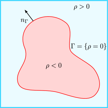
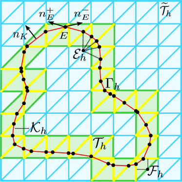
Figure 1. Domain set-up

We observe that the active background mesh $\mathcal{T}_{h}$ gives raise to a discrete or approximate $h$-tubular neighborhood of $\Gamma_{h}$, which we denote by

$$N_{h}=\cup_{T\in\mathcal{T}_{h}}T$$ (2.18)

Note that for all elements $T\in\mathcal{T}_{h}$ there is a neighbor $T^{\prime}\in\mathcal{T}_{h}$ such that $T$ and $T^{\prime}$ share a face.

Finally, let

$$V_{h}=\bigoplus_{T\in\mathcal{T}_{h}}P_{1}(T)$$ (2.19)

be the space of discontinuous piecewise linear polynomials defined on $\mathcal{T}_{h}$ and define the subspace

$$V_{h,0}=\{v\in V_{h}:\lambda_{\Gamma_{h}}(v)=0\}$$ (2.20)

consisting of those $v\in V_{h}$ with zero average $\lambda_{\Gamma_{h}}(v)=\int_{\Gamma_{h}}v$. Note that $V_{h,0}$ can be considered as the discrete version of $H^{1}(\Gamma)/\mathbb{R}$.

2.4. Discontinuous Galerkin Method

Before we formulate the cut discontinuous Galerkin method for the Laplace-Beltrami problem (2.7), we introduce the notation of average and jump first. As the co-normal vectors $n_{E}^{\pm}$ are generally not collinear, the average flux for a vector-valued, piecewise continuous function $\sigma$ on $\mathcal{K}_{h}$ is defined by

$$\langle{\sigma}\rangle|_{E} =\sigma_{E}^{+}\cdot n^{+}_{E}-\sigma_{E}^{-}\cdot n^{-}_{E}$$ (2.21)

while for any, possibly vector-valued, piecewise continuous function $w$ on $\mathcal{K}_{h}$, the jump across an interior edge $E\in\mathcal{E}_{h}$ is defined by

$$[w]|_{E} =w_{E}^{+}-w_{E}^{-}$$ (2.22)

with $w(x)^{\pm}=\lim_{t\rightarrow 0^{+}}w(x-tn_{E}^{\pm})$. Similarly, the jump across an interior face $F\in\mathcal{F}_{h}$ is given by

$$[w]|_{F} =w_{F}^{+}-w_{F}^{-}.$$ (2.23)

Next, we define the bilinear form $A_{h}(\cdot,\cdot)$ by

$$A_{h}(v,w)=a_{h}(v,w)+j_{h}(v,w)\quad\forall v,w\in V_{h}$$ (2.24)

with

$$a_{h}(v,w) =\sum_{K\in\mathcal{K}_{h}}(\nabla_{\Gamma_{h}}v,\nabla_{\Gamma_{h}}w)_{K}$$

$$\qquad-\sum_{E\in\mathcal{E}_{h}}(\langle{\nabla v}\rangle,[w])_{E}-\sum_{E\in\mathcal{E}_{h}}([v],\langle{\nabla w}\rangle)_{E}$$

$$\qquad+\sum_{E\in\mathcal{E}_{h}}\beta_{E}h^{-1}([v],[w])_{E}$$ (2.25)

$$j_{h}(v,w) =\sum_{F\in\mathcal{F}_{h}}\beta_{F}h^{-2}([v],[w])_{F}+\gamma(n_{F}\cdot[\nabla v],n_{F}\cdot[\nabla w])_{F}$$ (2.26)

where $\beta_{E},\beta_{F},\gamma$ are positive parameters. The right hand side is given by linear form

$$l_{h}(v)=(f^{e},v)_{\Gamma_{h}}$$ (2.27)

Then the cut discontinuous Galerkin finite element method for the Laplace-Beltrami problem (2.7) takes the form: find $u_{h}\in V_{h,0}$ such that

$$A_{h}(u_{h},v)=l_{h}(v)\quad\forall v\in V_{h,0}$$ (2.28)

We conclude this section by introducing suitable norms for the forthcoming stability and error analysis. Here and throughout this work, any norm $\|\cdot\|_{\mathcal{P}_{h}}$ involving a collection of geometric entities $\mathcal{P}_{h}$ is defined in the usual way, i.e., by summing over all entities: $\|\cdot\|_{\mathcal{P}_{h}}^{2}=\sum_{P\in\mathcal{P}_{h}}\|\cdot\|_{P}^{2}$. For the discrete energy norm associated to the weak formulation (2.28) we chose

$$|\mspace{-1.0mu}|\mspace{-1.0mu}|v|\mspace{-1.0mu}|\mspace{-1.0mu}|_{h}^{2} =\|\nabla_{\Gamma_{h}}v\|^{2}_{\mathcal{K}_{h}}+\|h^{-1/2}[v]\|^{2}_{\mathcal{E}_{h}}+\|h^{-1}[v]\|^{2}_{\mathcal{F}_{h}}+\|n_{F}\cdot[\nabla v]\|^{2}_{\mathcal{F}_{h}}$$ (2.29)

and for the function space $(H^{2}(\Gamma))^{e}+V_{h}$, we define

$$|\mspace{-1.0mu}|\mspace{-1.0mu}|v|\mspace{-1.0mu}|\mspace{-1.0mu}|_{\ast,h}^{2}=|\mspace{-1.0mu}|\mspace{-1.0mu}|v|\mspace{-1.0mu}|\mspace{-1.0mu}|_{h}^{2}+\|h^{1/2}\langle{\nabla_{\Gamma_{h}}v}\rangle\|_{\mathcal{E}_{h}}^{2}$$ (2.30)

For convenience, the part of the energy norm associated with the face terms is summarized by the notation

$$|\mspace{-1.0mu}|\mspace{-1.0mu}|v|\mspace{-1.0mu}|\mspace{-1.0mu}|^{2}_{\mathcal{F}_{h}}=\|h^{-1}[v]\|^{2}_{\mathcal{F}_{h}}+\|n_{F}\cdot[\nabla v]\|^{2}_{\mathcal{F}_{h}}$$ (2.31)

Although it is not obvious from the definition, we will later prove in that the discrete energy norm (2.29) indeed defines a norm on $V_{h,0}$, see Corollary 5.27.

Remark 2.1.

We point that thanks to inverse estimate (4.8), the edge-based penalty term appearing in (2.25) can be controlled by its face-based counterpart in the stabilization form (2.26). More precisely it holds

$$\|h^{-1/2}[u]\|_{\mathcal{E}_{h}}\lesssim\|h^{-1}[u]\|_{\mathcal{F}_{h}}$$ (2.32)

and consequently, one might simplify formulation (2.25) by setting $\beta_{E}=0$ at the expanse of possibly requiring a larger value for $\beta_{F}$.

2.5. Lifted Discontinuous Galerkin Form

The mismatch of the smooth surface $\Gamma$ and its discrete counterpart $\Gamma_{h}$ gives raise to a geometric variational crime in the proposed discretization scheme which must be accounted for in the forthcoming a priori analysis. An important instrument in assessing the error introduced by this variational crime will be the following lifted version of the bilinear form (2.25):

$$a_{h}^{l}(v,w) =\sum_{K^{l}\in\mathcal{K}^{l}_{h}}(\nabla_{\Gamma}v,\nabla_{\Gamma}w)_{K^{l}}$$ (2.33)

$$\qquad-\sum_{E^{l}\in\mathcal{E}^{l}_{h}}(\langle{\nabla v}\rangle,[w])_{E^{l}}-\sum_{E^{l}\in\mathcal{E}^{l}_{h}}([v],\langle{\nabla w}\rangle)_{E^{l}}$$

$$\qquad+\sum_{E^{l}\in\mathcal{E}^{l}_{h}}\beta_{E}h^{-1}([v],[w])_{E^{l}}$$ (2.34)

where, referring to the notation in Section 2.4, the average $\langle\cdot\rangle$ is taken with respect to $n_{E^{l}}^{\pm}(x)\in T_{x}K^{l,\pm}$; that is the unique co-normal vector which points outwards $K^{l,\pm}$ and is orthogonal to both the surface $n_{\Gamma}(x)$ and the tangential space $T_{x}E^{l,\pm}$. With the definition of the lifted discontinuous Galerkin form, it is clear that the solution $u$ of problem (2.7) satisfies the following weak problem:

$$a_{h}^{l}(u,v)=l(v)\quad\forall v\in V_{h}^{l}$$ (2.35)

For $v\in H^{2}(\Gamma)+V_{h}^{l}$, the natural energy norm associated with this weak form is given by

$$|\mspace{-1.0mu}|\mspace{-1.0mu}|v|\mspace{-1.0mu}|\mspace{-1.0mu}|_{\ast}^{2} =\|\nabla_{\Gamma}v\|^{2}_{\mathcal{K}_{h}^{l}}+\|h^{-1/2}[v]\|^{2}_{\mathcal{E}_{h}^{l}}+\|h^{1/2}\langle\nabla_{\Gamma}v\rangle\|^{2}_{\mathcal{E}_{h}^{l}}$$ (2.36)

3. Domain Perturbation Related Estimates

The aim of this section is to collect the appropriate geometric estimates which are necessary to quantify the error introduced by the geometric variational crime, i.e., the piecewise linear approximation of the smooth surface $\Gamma$. While developing face and edge-related estimates simultaneously, we essentially follow the presentations in Dziuk [13], Olshanskii et al. [32], Dziuk and Elliott [14] and include without detailed proofs those results which are well known. Here and throughout the remaining work, we write $(\cdot,\cdot)_{\mathbb{R}^{d}}$ and $\|\cdot\|_{\mathbb{R}^{d}}$ to denote the standard scalar product and its associate norm in $\mathbb{R}^{d}$.

3.1. Gradient of Lifted and Extended Functions

Derivatives of extend and lifted functions can easily be computed by the chain rule, once the derivative of the closest point projection is known. Using the fact that $\nabla\rho=n_{\Gamma}$, the derivative of the closest point projection computes to

$$Dp=I-n_{\Gamma}\otimes n_{\Gamma}-\rho\nabla\otimes\nabla\rho$$ (3.1)

where $\mathcal{H}=\nabla\otimes\nabla\rho=\nabla n_{\Gamma}$ denotes the Hessian of the signed distance function. The symmetry of the Hessian and the projection ${P}_{\Gamma}$ together with simple fact that $0=\nabla\|n_{\Gamma}\|_{\mathbb{R}^{d}}^{2}=2\nabla n_{\Gamma}^{T}n_{\Gamma}$ implies that $\mathcal{H}n_{\Gamma}=0$ and $(n_{\Gamma}\otimes n_{\Gamma})\mathcal{H}=0$ and therefore that $\mathcal{H}{P}_{\Gamma}=\mathcal{H}={P}_{\Gamma}\mathcal{H}$. This allows to rewrite 3.1 as

$$Dp={P}_{\Gamma}(I-\rho\mathcal{H})={P}_{\Gamma}-\rho\mathcal{H}$$ (3.2)

and thus

$$Dv^{e}=D(v\circ p)=DvDp=DvP_{\Gamma}(I-\rho\mathcal{H})$$ (3.3)

Exploiting the self-adjointness of ${P}_{\Gamma}$, ${P}_{\Gamma_{h}}$, and $\mathcal{H}$, we have for any vector $a\in\mathbb{R}^{d}$

$$(\nabla_{\Gamma_{h}}v^{e},a)_{\mathbb{R}^{d}} =(\nabla v^{e},{P}_{\Gamma_{h}}a)_{\mathbb{R}^{d}}$$

$$=Dv^{e}{P}_{\Gamma_{h}}a=Dv{P}_{\Gamma}(I-\rho\mathcal{H}){P}_{\Gamma_{h}}a=(\nabla v,{P}_{\Gamma}(I-\rho\mathcal{H}){P}_{\Gamma_{h}}a$$ (3.4)

$$=({P}_{\Gamma_{h}}(I-\rho\mathcal{H}){P}_{\Gamma}\nabla v,a)_{\mathbb{R}^{d}}$$ (3.5)

that is

$$\nabla_{\Gamma_{h}}v^{e}=B^{T}\nabla_{\Gamma}v$$ (3.6)

where we introduced the invertible linear mapping

$$B=P_{\Gamma}(I-\rho H)P_{\Gamma_{h}}:T_{x}(K)\to T_{p(x)}(\Gamma)$$ (3.7)

which maps the tangential space of $K$ at $x$ to the tangential space of $\Gamma$ at $p(x)$. Setting $v=w^{l}$ and using the identity $(w^{l})^{e}=w$, we immediately get that

$$\nabla_{\Gamma}w^{l}=B^{-T}\nabla_{\Gamma_{h}}w$$ (3.8)

for any elementwise differentiable function $w$ on $\Gamma_{h}$ lifted to $\Gamma$. From its definition (3.7), it is easy to derive norm bounds for operators involving $B$ once $\mathcal{H}$ can be controlled. We recall from [18, Lemma 14.7] that for $x\in U_{\delta_{0}}(\Gamma)$, the Hessian $\mathcal{H}$ admits a representation

$$\mathcal{H}(x)=\sum_{i=1}^{d}\frac{\kappa_{i}^{e}}{1+\rho(x)\kappa_{i}^{e}}a_{i}^{e}\otimes a_{i}^{e}$$ (3.9)

where $\kappa_{i}$ are the principal curvatures with corresponding principal curvature vectors $a_{i}$. Thus

$$\|\mathcal{H}\|_{L^{\infty}(U_{\delta_{0}}(\Gamma))}\lesssim 1$$ (3.10)

for $\delta_{0}>0$ small enough and as an almost immediate consequence, we have the following estimates summarized in

Lemma 3.1.

It holds

$$\|B\|_{L^{\infty}(\Gamma_{h})}\lesssim 1,\quad\|B^{-1}\|_{L^{\infty}(\Gamma)}\lesssim 1,\quad\|P_{\Gamma}-BB^{T}\|_{L^{\infty}(\Gamma)}\lesssim h^{2}$$ (3.11)

Proof.

The proof is standard, see Dziuk and Elliott [14], and only sketched here for completeness. The first two bounds follow directly from (3.7) and  (3.10) together with the assumption $\|\rho\|_{L^{\infty}(\Gamma_{h})}\lesssim h^{2}$. Similarly, it follows that ${P}_{\Gamma}-BB^{T}={P}_{\Gamma}-{P}_{\Gamma}{P}_{\Gamma_{h}}{P}_{\Gamma}+O(h^{2}).$ An easy calculation now shows that ${P}_{\Gamma}-{P}_{\Gamma}{P}_{\Gamma_{h}}{P}_{\Gamma}={P}_{\Gamma}({P}_{\Gamma}-{P}_{\Gamma_{h}})^{2}{P}_{\Gamma}$ from which the desired bound follows by observing that ${P}_{\Gamma}-{P}_{\Gamma_{h}}=(n-n_{h})\otimes n+n_{h}\otimes(n-n_{h})$ and thus $\|({P}_{\Gamma}-{P}_{\Gamma_{h}})^{2}\|_{L^{\infty}(\Gamma_{h})}\lesssim\|n-n_{h}\|_{L^{\infty}(\Gamma_{h})}^{2}\lesssim h^{2}$ ∎

3.2. Change of the Integration Domain

Next, we derive estimates for the change of the Riemannian measure when surface and edge integrals are lifted from the discrete surface to the continuous surface and vice versa. For this purpose, we define the quotient of measures $|B|_{d-1}$ and $|B|_{d-2}$ by

$$\,\mathrm{d}K^{l}=|B|_{d-1}\,\mathrm{d}K,\quad\,\mathrm{d}E^{l}=|B|_{d-2}\,\mathrm{d}E$$ (3.12)

where $\,\mathrm{d}K$ and $\,\mathrm{d}E$ denotes the measure on $K\in\mathcal{K}_{h}$ and $E\in\mathcal{E}_{h}$, respectively, while the corresponding measures on the lifted entities $K^{l}\in\mathcal{K}_{h}^{l}$ and $E^{l}\in\mathcal{E}_{h}^{l}$ are denoted by $\,\mathrm{d}K^{l}$ and $\,\mathrm{d}E^{l}$, respectively. Picking an element $K$ and one of its boundary edges $E$ together with its outer co-normal $n_{E}$, we can assume (after some rigid motion) that $K\subset\mathbb{R}^{d-1}\times\{0\}$ and $E\subset\mathbb{R}^{d-2}\times\{0,0\}$ and that $n_{K}=e_{d}$ and $n_{E}=e_{d-1}$. In this coordinate system, we have $\,\mathrm{d}K=\,\mathrm{d}x_{1}\dots\,\mathrm{d}x_{d-1}$ and $\,\mathrm{d}E=\,\mathrm{d}x_{1}\dots\,\mathrm{d}x_{d-2}$.

Recall that for any smooth parametrized $k$-dimensional sub-manifold $M\subset\mathbb{R}^{d}$ together with a smooth parametrization $p:U\subset\mathbb{R}^{k}\to\mathbb{R}^{d}$ satisfying $p(U)=M$, the integral $\int_{M}f\,\mathrm{d}M$ of a function $f:M\to\mathbb{R}$ is given by

$$\int_{M}f\,\mathrm{d}M=\int_{U}f(p(x))\sqrt{\det(g_{ij}(x))}\,\mathrm{d}x,$$ (3.13)

where $g_{ij}=(\partial_{i}p,\partial_{j}p)_{\mathbb{R}^{d}}$ $i,j=1,\dots,k$ is the first fundamental form of $M$ in local coordinates. Considering the cases $M=K^{l}$, $U=K$ and $M=E^{l}$ and $U=E$ with the closest point projection $p$ as parametrization, we see that $|B|_{d-1}$ and $|B|_{d-2}$ are precisely given by the $d-1$ and $d-2$ volumes

$$|B|_{d}=\sqrt{\det((g_{ij}))_{i,j=1}^{d-1}}$$ (3.14)

$$|B|_{d-2}=\sqrt{\det((g_{ij}))_{i,j=1}^{d-2}}$$ (3.15)

Instead of calculating these volumes exactly, we derive a simple asymptotic representation in $h$. Combining the representation (3.2) of $Dp$ with the fact that the choice of our coordinate system implies

$$n_{\Gamma}^{i}=(n_{\Gamma},e_{i})_{\mathbb{R}^{d}}\lesssim h,\quad i=1,\dots,d-1,\text{ and thus}\quad n_{\Gamma}^{d}\sim 1+O(h^{2})$$ (3.16)

allows us to derive an asymptotic expression for the coefficients $g_{ij}$ for $i,j=1,\dots,d-1$:

$$g_{ij} =((P_{\Gamma}-\rho\mathcal{H})e_{i},(P_{\Gamma}-\rho\mathcal{H})e_{i})_{\mathbb{R}^{d}}$$ (3.17)

$$=(P_{\Gamma}e_{i},P_{\Gamma}e_{i})_{\mathbb{R}^{d}}+O(h^{2})$$ (3.18)

$$=\delta_{ij}-n_{\Gamma}^{i}n_{\Gamma}^{j}+O(h^{2})$$ (3.19)

$$\sim\delta_{ij}+O(h^{2}).$$ (3.20)

Consequently, $\sqrt{\det(g_{ij})}\sim\sqrt{1+O(h^{2})}\sim 1+O(h^{2})$ and thus

$$|B|_{d}\sim 1+O(h^{2})$$ (3.21)

$$|B|_{d-1}\sim 1+O(h^{2})$$ (3.22)

which leads directly to the bounds summarized in the next Lemma.

Lemma 3.2.

The following estimates hold

$$\|1-|B|_{d-1}\|_{L^{\infty}(\mathcal{K}_{h})} \lesssim h^{2}, \qquad\||B|_{d}\|_{L^{\infty}(\mathcal{K}_{h})} \lesssim 1, \qquad\||B|_{d}^{-1}\|_{L^{\infty}(\mathcal{K}_{h})} \lesssim 1$$ (3.23)

$$\|1-|B|_{d-2}\|_{L^{\infty}(\mathcal{E}_{h})} \lesssim h^{2}, \qquad\||B|_{d-2}\|_{L^{\infty}(\mathcal{E}_{h})} \lesssim 1, \qquad\||B|_{d}^{-1}\|_{L^{\infty}(\mathcal{E}_{h})} \lesssim 1$$ (3.24)

We point out that estimates similar to (3.24) were derived in the finite volume context in Giesselmann and Müller [17] and used in Dedner et al. [11].

Next, we note that by combining the estimates for the operator norms (3.11) and for the metric distortion factors (3.23)–(3.24), the following norm equivalences can be obtained:

Lemma 3.3.

Let $v\in L^{2}(\mathcal{P}_{h})$ and $w\in L^{2}(\mathcal{P}_{h}^{l})$ for $\mathcal{P}_{h}\in\{\mathcal{K}_{h},\mathcal{E}_{h}\}$. Then it holds

$$\|v^{l}\|_{\mathcal{P}_{h}^{l}}\sim\|v\|_{\mathcal{P}_{h}},\qquad\|w\|_{\mathcal{P}_{h}^{l}}\sim\|w^{e}\|_{\mathcal{P}_{h}}$$ (3.25)

If in addition $v\in H^{1}(\mathcal{K}_{h})$ and $w\in H^{1}(\mathcal{K}_{h}^{l})$ the following equivalences are satisfied

$$\|\nabla_{\Gamma}v^{l}\|_{\mathcal{K}_{h}^{l}}\sim\|\nabla_{\Gamma_{h}}v\|_{\mathcal{K}_{h}},\qquad\|\nabla_{\Gamma}w\|_{\mathcal{K}_{h}^{l}}\sim\|\nabla_{\Gamma_{h}}w^{e}\|_{\mathcal{K}_{h}}$$ (3.26)

Before we proceed, let us note that the measure quotients  (3.14)–(3.22) can be equivalently expressed using the exterior product of the tangential vectors $\partial_{i}p$, $i=1,\dots,d-1$ and the surface normal $n_{\Gamma}$. More precisely,

$$|B|_{d-1} =\|\partial_{1}p\wedge\ldots\wedge\partial_{d-1}p\|$$ (3.27)

$$|B|_{d-2} =\|\partial_{1}p\wedge\ldots\partial_{d-2}p\wedge n_{\Gamma}\|$$ (3.28)

where for given vectors $v_{1},\dots,v_{d-1}\in\mathbb{R}^{d}$ the outer product $v_{1}\wedge\ldots\wedge v_{d-1}$ is the unique vector satisfying

$$\det(v_{1},\ldots,v_{d-1},w)=(v_{1}\wedge\ldots\wedge v_{d-1},w)_{\mathbb{R}^{d}}\quad\forall w\in\mathbb{R}^{d}.$$ (3.29)

With this in mind we can now easily estimate the deviation of the lifted co-normal vector $n_{E}^{l}$ from the co-normal vector $n_{E^{l}}$ associated with the lifted edge $E^{l}$.

Lemma 3.4.

It holds

$$\|B^{l}n_{E}^{l}-|B|_{d-2}n_{E^{l}}\|_{L^{\infty}(E^{l})}\lesssim h^{2},$$ (3.30)

Proof.

Expanding the scaled co-normal and lifted discrete co-normal vectors in the standard orthonormal basis $e_{1},\ldots,e_{d}$, it suffices to show that the resulting expansion coefficients satisfy the estimates

$$(B^{l}n_{E}^{l}-|B|_{d-2}^{l}n_{E^{l}},e_{i})_{\mathbb{R}^{d}}\lesssim h^{2}\quad i=1,\ldots,d.$$ (3.31)

To compute $(B^{l}n_{E}^{l},e_{i})_{\mathbb{R}^{d}}$, we simply calculate

$$(B^{l}n_{E}^{l},e_{i})_{\mathbb{R}^{d}} =({P}_{\Gamma}(I-\rho\mathcal{H})e_{d-1},e_{i})_{\mathbb{R}^{d}}=({P}_{\Gamma}e_{d-1},e_{i})_{\mathbb{R}^{d}}+O(h^{2})$$ (3.32)

$$=\delta_{d-1,i}-n_{\Gamma}^{d-1}n_{\Gamma}^{i}+O(h^{2})$$ (3.33)

$$=\begin{cases}O(h^{2}),\quad i=1,\ldots d-2\\ 1+O(h^{2}),\quad i=d-1\\ -n_{\Gamma}^{d-1}n_{\Gamma}^{d}+O(h^{2}),\quad i=d\end{cases}$$ (3.34)

Now turning to $-(|B|_{d-2}^{l}n_{E^{l}},e_{i})_{\mathbb{R}^{d}}$, we observe that due to (3.28), the fact that $-n_{E}^{l}$ is pointing inwards and $n_{E}\perp\partial_{1}p,\ldots,\partial_{d-2}p,n_{\Gamma}$, we have

$$-|B|_{d-2}n_{E^{l}}=\partial_{1}p\wedge\dots\wedge\partial_{d-2}p\wedge n_{\Gamma},$$ (3.35)

and therefore by definition of the exterior product (3.29)

$$-(|B|_{d-2}n_{E^{l}},e_{i})_{\mathbb{R}^{d}} =\det(Dpe_{1},\ldots,Dpe_{d-2},n_{\Gamma},e_{i})$$ (3.36)

$$=\det({P}_{\Gamma}e_{1},\ldots,{P}_{\Gamma}e_{d-2},n_{\Gamma},e_{i})+O(h^{2})$$ (3.37)

$$=\det(e_{1},\ldots,e_{d-2},n_{\Gamma},e_{i})+O(h^{2})$$ (3.38)

$$=\begin{cases}0+O(h^{2}),\quad i=1,\ldots,d-2,\\ -n_{\Gamma}^{d}+O(h^{2})=-1+O(h^{2}),\quad i=d-1,\\ n_{\Gamma}^{d-1}+O(h^{2})\quad i=d.\end{cases}$$ (3.39)

Now adding (3.34) and (3.39) we arrive at the desired estimate by observing that $n_{\Gamma}^{d-1}-n_{\Gamma}^{d-1}n_{\Gamma}^{d}=n_{\Gamma}^{d-1}(1-n_{\Gamma}^{d})=n_{\Gamma}^{d-1}\cdot O(h^{2})$. ∎

The previous lemma roughly states that push-forwarding a properly scaled discrete co-normal vector results in a good approximation of the co-normal vector field along the lifted edge. As a result we can prove the final lemma of this section.

Lemma 3.5.

For $v\in H^{1}(\Gamma)^{e}+V_{h}$ it holds

$$|\mspace{-1.0mu}|\mspace{-1.0mu}|v^{l}|\mspace{-1.0mu}|\mspace{-1.0mu}|_{\ast}\lesssim|\mspace{-1.0mu}|\mspace{-1.0mu}|v|\mspace{-1.0mu}|\mspace{-1.0mu}|_{\ast,h}$$ (3.40)

Proof.

We only sketch the proof. Recalling the norm definitions (2.29) and (2.36) and the norm equivalences from Lemma 3.5, it remains to show that

$$\|\langle{\nabla_{\Gamma}v^{l}}\rangle\|_{E^{l}}\sim\|\langle{\nabla v}\rangle\|_{E}$$ (3.41)

where the mean incorporates the co-normal of the lifted edge $E^{l}$ and the discrete edge $E$, respectively. Lifting the $\langle{\nabla_{\Gamma_{h}}v}\rangle$ to $\Gamma$, equivalence (3.41) can easily proven as in (6.16)–(6.18) by using the previous lemma to bound the deviation of the lifted discrete co-normal flux from the co-normal flux of the lifted edges. ∎

4. Approximation Properties

Before we turn to the stability and a priori analysis in the next two sections, we here collect some standard inequalities and establish the appropriate interpolation estimates which will be frequently used throughout the remaining work.

4.1. Useful Inequalities

First, we recall the following trace inequality for $v\in H^{1}(\mathcal{T}_{h})$

$$\|v\|_{\partial T}\lesssim h^{-1/2}\|v\|_{T}+h^{1/2}\|\nabla v\|_{T}\quad\forall\,T\in\mathcal{T}_{h}$$ (4.1)

If the intersection $\Gamma\cap T$ does not coincide with a boundary face of the mesh then the corresponding inequality

$$\|v\|_{\Gamma\cap T}\lesssim h^{-1/2}\|v\|_{T}+h^{1/2}\|\nabla v\|_{T}\quad\forall\,T\in\mathcal{T}_{h}$$ (4.2)

holds whenever the surface $\Gamma$ is reasonably resolved by the background mesh, i.e. the mesh size is chosen in accordance with the local curvature, see Hansbo et al. [23] for a proof. Correspondingly, since the skeleton $\mathcal{F}_{h}$ consists of shape-regular faces, we have

$$\|v\|_{E\cap F}\lesssim h^{-1/2}\|v\|_{F}+h^{1/2}\|\nabla v\|_{F}\quad\forall\,E\in\mathcal{E}_{h},\;\forall\,F\in\mathcal{F}_{h}$$ (4.3)

and if we iterate using 4.1 we see that for $v\in H^{2}(\mathcal{T}_{h})$

$$\|v\|_{E\cap F}\lesssim h^{-1}\|v\|_{T}+\|\nabla v\|_{T}+h\|\nabla\otimes\nabla v\|_{T}\quad\forall\,E\in\mathcal{E}_{h},\;\forall\,F\in\mathcal{F}_{h}$$ (4.4)

In the following, we will also need the some well-known inverse estimates for $v_{h}\in V_{h}$:

$$\|\nabla v_{h}\|_{T}\lesssim h^{-1}\|v_{h}\|_{T}\quad\forall\,T\in\mathcal{T}_{h}$$ (4.5)

$$\|v_{h}\|_{\partial T}\lesssim h^{-1/2}\|v_{h}\|_{T},\qquad\|\nabla v_{h}\|_{\partial T}\lesssim h^{-1/2}\|\nabla v_{h}\|_{T}\quad\forall\,T\in\mathcal{T}_{h}$$ (4.6)

and the following “cut versions” (note that $K\cap T\not\subseteq\partial T$, $E\cap F\not\subseteq\partial F$):

$$\|v_{h}\|_{K\cap T} \lesssim h^{-1/2}\|v_{h}\|_{T}, \qquad\|\nabla v_{h}\|_{K\cap T} \lesssim h^{-1/2}\|\nabla v_{h}\|_{T} \quad\forall\,K\in\mathcal{K}_{h},\;\forall\,T\in\mathcal{T}_{h}$$ (4.7)

$$\|v_{h}\|_{E\cap F} \lesssim h^{-1/2}\|v_{h}\|_{F}, \qquad\|\nabla v_{h}\|_{E\cap F} \lesssim h^{-1/2}\|\nabla v_{h}\|_{F} \quad\forall\,E\in\mathcal{E}_{h},\;\forall\,F\in\mathcal{F}_{h}$$ (4.8)

which are an immediate consequence of similar inverse estimates presented in Hansbo et al. [23].

4.2. Interpolation Operators

Next, we recall from Scott and Zhang [35] that for $v\in H^{m}(\mathcal{T}_{h})$, the standard Scott-Zhang interpolant $I_{h}:L^{2}(N_{h})\rightarrow V_{h}$ satisfies the local interpolation estimates

$$\|v-I_{h}v\|_{k,T} \lesssim h^{l-k}|v|_{l,\omega(T)}, \quad 0\leqslant k\leqslant l\leqslant\min\{2,m\}\quad \forall\,T\in\mathcal{T}_{h}$$ (4.9)

$$\|v-I_{h}v\|_{l,F} \lesssim h^{l-k-1/2}|v|_{l,\omega(F)}, \quad 0\leqslant k\leqslant l-1/2\leqslant\min\{2,m\}-1/2\quad \forall\,F\in\mathcal{F}_{h}$$ (4.10)

where $\omega(T)$ denotes the patch of all elements sharing a vertex with $T$. The patch $\omega(F)$ is defined analoguously. Before we introduce a suitable interpolation operator $I_{h}:H^{m}(\Gamma)\to V_{h}$, we note that by the coarea-formula (cf. Evans and Gariepy [16])

$$\int_{U_{\delta}}f(x)\,dx=\int_{-\delta}^{\delta}\left(\int_{\Gamma(r)}f(y,r)\,\mathrm{d}\Gamma_{r}(y)\right)\,\mathrm{d}r$$

the extension operator $v^{e}$ defines a bounded operator $H^{m}(\Gamma)\ni v\mapsto v^{e}\in H^{m}(U_{\delta}\Gamma))$ satisfying the stability estimate

$$\|v^{e}\|_{k,U_{\delta}(\Gamma)}\lesssim\delta^{1/2}\|v\|_{k,\Gamma},\qquad 0\leqslant k\leqslant m$$ (4.11)

for $0<\delta\leqslant\delta_{0}$ where the hidden constant depends only on the curvature of $\Gamma$. With the help of the extension operator, we construct an interpolation operator $I_{h}:H^{m}(\Gamma)\to V_{h}$ by setting $I_{h}v=I_{h}v^{e}$ where we the liberty of using the same symbol. Choosing $\delta_{0}\sim h$, it follows directly from combining the interpolation estimate (4.10) and the stability estimate (4.11) that the following lemma holds:

Lemma 4.1.

Setting $e_{I}=v^{e}-I_{h}v^{e}$ then for $v\in H^{2}(\Gamma)$, it holds that

$$\sum_{F\in\mathcal{F}}\bigl{(}h^{-2}\|e_{I}\|_{F}^{2}+\|\nabla e_{I}\|_{F}^{2}+h^{2}\|\nabla\otimes\nabla e_{I}\|_{F}^{2}\bigr{)}\lesssim h^{2}\|v\|_{2,\Gamma}^{2}$$ (4.12)

The interpolation operator satisfies the following interpolation error estimate with respect to the discrete energy norm

Lemma 4.2.

For $v\in H^{2}(\Gamma)$, it holds that

$$|\mspace{-1.0mu}|\mspace{-1.0mu}|v^{e}-I_{h}v^{e}|\mspace{-1.0mu}|\mspace{-1.0mu}|_{\ast,h}+|\mspace{-1.0mu}|\mspace{-1.0mu}|v^{e}-I_{h}v^{e}|\mspace{-1.0mu}|\mspace{-1.0mu}|_{\mathcal{F}_{h}} \lesssim h\|v\|_{2,\Gamma}$$ (4.13)

Proof.

By definition

$$|\mspace{-1.0mu}|\mspace{-1.0mu}|v^{e}-I_{h}v^{e}|\mspace{-1.0mu}|\mspace{-1.0mu}|_{\ast,h}^{2} =(\nabla_{\Gamma_{h}}(v^{e}-I_{h}v^{e}),\nabla_{\Gamma_{h}}(v^{e}-I_{h}v^{e}))_{\mathcal{K}_{h}}$$

$$\quad+h\|\nabla_{\Gamma_{h}}(v^{e}-I_{h}v^{e})\cdot n_{E,h}\|_{\mathcal{E}_{h}}^{2}+h^{-1}\|v^{e}-I_{h}v^{e}\|_{\mathcal{E}_{h}}$$ (4.14)

$$=I+II+III$$ (4.15)

which we estimate next.
Term I. Successively employing the trace inequality (4.1), the interpolation estimate (4.9) and the stability bound (4.11) with $\delta_{0}\sim h$, it follows that

$$I =\sum_{T\in\mathcal{T}_{h}}(\nabla_{\Gamma_{h}}(v^{e}-I_{h}v^{e}),\nabla_{\Gamma_{h}}(v^{e}-I_{h}v^{e}))_{\Gamma_{h}\cap T}$$ (4.16)

$$\lesssim\sum_{T\in\mathcal{T}_{h}}\|\nabla(v^{e}-I_{h}v^{e})\|^{2}_{T\cap\Gamma_{h}}$$ (4.17)

$$\lesssim\sum_{T\in\mathcal{T}_{h}}\bigl{(}h^{-1}\|\nabla(v^{e}-I_{h}v^{e})\|^{2}_{T}+h\|\nabla\otimes\nabla(v^{e}-I_{h}v^{e})\|^{2}_{T}\bigr{)}$$ (4.18)

$$\lesssim\sum_{T\in\mathcal{T}_{h}}h\|v^{e}\|^{2}_{2,\omega(T)}$$ (4.19)

$$\lesssim h\|v^{e}\|^{2}_{2,U_{\delta_{0}}(\Gamma)}$$ (4.20)

$$\lesssim h^{2}\|v\|^{2}_{2,\Gamma}$$ (4.21)

Term II. To estimate the second contribution, we employ the trace inequaltiy (4.3) to pass from $E$ to $F$ which in combination with (4.10) and (4.11) gives

$$II \lesssim\sum_{E\in\mathcal{E}_{h}}h||\nabla_{\Gamma_{h}}(v^{e}-I_{h}v^{e})\|_{E}^{2}$$ (4.22)

$$\lesssim\sum_{E\in\mathcal{E}_{h}}\bigl{(}||\nabla(v^{e}-I_{h}v^{e})\|_{F}^{2}+h^{2}||\nabla\otimes\nabla(v^{e}-I_{h}v^{e})\|_{F}^{2}\bigr{)}$$ (4.23)

$$\lesssim h^{2}\|v\|^{2}_{2,\Gamma}$$ (4.24)

Term III. Applying the same reasoning as for the estimate of Term II, we obtain

$$III\lesssim\sum_{E\in\mathcal{E}_{h}}h^{-1}\|e_{I}\|_{E}\lesssim\sum_{F\in\mathcal{F}_{h}}\big{(}h^{-2}\|e_{I}\|_{F}^{2}+\|\nabla e_{I}\|_{F}^{2}\bigr{)}\lesssim h^{2}\|v\|^{2}_{2,\Gamma}$$ (4.25)

To estimate the remaining term $|\mspace{-1.0mu}|\mspace{-1.0mu}|e_{I}|\mspace{-1.0mu}|\mspace{-1.0mu}|_{\mathcal{F}_{h}}$, we simply apply the previous Lemma 4.1 to arrive at the desired bound. ∎

We conclude this section by briefly reviewing the the Oswald interpolator, cf. Burman et al. [4], which will be of particular use in establishing discrete Poincaré-type estimates in Section 5.2. By construction, $\mathcal{O}_{h}:\mathcal{P}_{dc}^{k}(\mathcal{T})\to\mathcal{P}_{c}^{k}(\mathcal{T}_{h})$, with $\mathcal{P}_{dc}^{k}(\mathcal{T}_{h})$ and $\mathcal{P}_{c}^{k}(\mathcal{T}_{h})$ denoting the space of discontinuous and continuous piecewise polynonials of order $k$. Therefore the Oswald interpolator can be thought of as a certain “smoothing operator” and the following lemma shows how the fluctuation $Id-\mathcal{O}_{h}$ can be controlled in terms of jumps on the faces.

Lemma 4.3.

For $v\in\mathcal{P}_{dc}^{k}(\mathcal{T}_{h})$, it holds that

$$\|\mathcal{O}_{h}(v)\|_{T} \lesssim\|v\|_{\omega(T)}$$ (4.26)

$$\|v-\mathcal{O}_{h}(v)\|_{T}^{2} \lesssim\sum_{F\in\mathcal{F}_{h}(T)}h\|[v]\|_{F}^{2}$$ (4.27)

where $\mathcal{F}_{h}(T)$ denotes the set of all faces $F\in\mathcal{F}_{h}$ with $F\cap T\neq\emptyset$.

A proof can be found in e.g. Burman et al. [4], together with the construction of the Oswald interpolator and a summary of some of its important properties.

5. Stability Estimates

In this section, we demonstrate that the bilinear form $a_{h}(\cdot,\cdot)+j_{h}(\cdot,\cdot)$ defined in Section 2.4 is both stable and coercive with respect to its associated energy norm. The proof of the coercivity result is based on a special discrete Poincaré inequality which shows that for discrete functions, various $L^{2}$ norms can be controlled by merely the tangential gradient and the semi-norm induced by stabilization form $j_{h}(\cdot,\cdot)$. As a major instrument in establishing such Poincaré inequalities, we start by reviewing certain geometric covering relations of the active background mesh and a certain stabilization mechanism provided by the bilinear form $j_{h}(\cdot,\cdot)$.

5.1. Fat Intersection Covering and Ghost Penalties

Since the surface geometry is represented on fixed background mesh, the active background mesh $\mathcal{T}_{h}$ might contain elements which barely intersects the discretized surface $\Gamma_{h}$. Such “small cut elements” typically prohibit the application of a whole set of well-known estimates, such as interpolation estimates and inverse inequalities, which typically rely on certain scaling properties. As a partial replacement for the lost scaling properties we here recall from Burman et al. [6] the concept of fat intersection coverings of $\mathcal{T}_{h}$.

In Burman et al. [6] it was proved that the active background mesh fulfills a fat intersection property which roughly states that for every element in $\mathcal{T}_{h}$ there is close-by element which has a significant intersection with $\Gamma_{h}$. More precisely, let $x$ be a point on $\Gamma$ and let $B_{\delta}(x)=\{y\in\mathbb{R}^{d}:|x-y|<\delta\}$ and $D_{\delta}=B_{\delta}(x)\cap\Gamma$. We define the sets of elements

$$\mathcal{K}_{\delta,x}=\{K\in\mathcal{K}_{h}:\overline{K}^{l}\cap D_{\delta}(x)\neq\emptyset\},\qquad\mathcal{T}_{\delta,x}=\{T\in\mathcal{T}_{h}:T\cap\Gamma_{h}\in\mathcal{K}_{\delta,x}\}$$ (5.1)

With $\delta\sim h$ we use the notation $\mathcal{K}_{h,x}$ and $\mathcal{T}_{h},x$. For each $\mathcal{T}_{h}$, $h\in(0,h_{0}]$ there is a set of points $\mathcal{X}_{h}$ on $\Gamma$ such that $\{\mathcal{K}_{h,x},x\in\mathcal{X}_{h}\}$ and $\{\mathcal{T}_{h,x},x\in\mathcal{X}_{h}\}$ are coverings $\mathcal{T}_{h}$ and $\mathcal{K}_{h}$ with the following properties:

• The number of set containing a given point $y$ is uniformly bounded

  $$\#\{x\in\mathcal{X}_{h}:y\in\mathcal{T}_{h,x}\}\lesssim 1\quad\forall\,y\in\mathbb{R}^{d}$$ (5.2)

  for all $h\in(0,h_{0}]$ with $h_{0}$ small enough.

• The number of elements in the sets $\mathcal{T}_{h,x}$ is uniformly bounded

  $$\#\mathcal{T}_{h,x}\lesssim 1\quad\forall\,x\in\mathcal{X}_{h}$$ (5.3)

  for all $h\in(0,h_{0}]$ with $h_{0}$ small enough, and each element in $\mathcal{T}_{h,x}$ shares at least one face with another element in $\mathcal{T}_{h,x}$.

• $\forall\,h\in(0,h_{0}]$ with $h_{0}$ small enough, and $\forall\,x\in\mathcal{X}_{h}$, $\exists T_{x}\in\mathcal{T}_{h,x}$ that has a large (fat) intersection with $\Gamma_{h}$ in the sense that

  $$|T_{x}|\sim h|T_{x}\cap\Gamma_{h}|=h|K_{x}|\quad\forall\,x\in\mathcal{X}_{h}$$ (5.4)

To make use of the fat intersection property, we will need the following lemma which describes how to the control of discrete functions on potentially small cut elements can be transferred to their close-by neighbors with large intersection by using the face-based stabilization terms appearing in $j_{h}(\cdot,\cdot)$.

Lemma 5.1.

Let $v$ be a discontinuous, piecewise linear function defined on a quasi-uniform mesh $\mathcal{T}_{h}$ consisting of element $\{T\}$ and consider a the macro-element $\mathcal{M}=T_{1}\cup T_{2}$ formed by any two elements $T_{1}$ and $T_{2}$ sharing a face $F$. Then

$$\|v\|_{T_{1}}^{2} \lesssim\|v\|_{T_{2}}^{2}+h\|[u]\|_{F}^{2}+h^{3}\|n_{F}\cdot[\nabla v]\|_{F}^{2}$$ (5.5)

$$\|\nabla v\|_{T_{1}}^{2} \lesssim\|\nabla v\|_{T_{2}}^{2}+h^{-1}\|[v]\|_{F}^{2}+h\|n_{F}\cdot[\nabla v]\|_{F}^{2}$$ (5.6)

with the hidden constant only depending on the quasi-uniformness parameter.

Proof.

A proof of the first estimate can be found in Massing et al. [29]. Setting $v=\nabla w$ in (5.5), the second inequality follows directly from the first one once the following face base inverse estimate is established:

$$\|[\nabla v]\|_{F}^{2}\lesssim\|n_{F}\cdot[\nabla v]\|_{F}^{2}+h^{-2}\|[v]\|_{F}^{2}$$ (5.7)

To prove (5.7), rewrite $\nabla v=n_{F}\cdot\nabla v+P_{F}\nabla v$ with $P_{F}=Id-n_{F}\otimes n_{F}$ and observe that the face tangential part of the gradient satisfies $\|[P_{F}\nabla u]\|_{F}^{2}\lesssim h^{-2}\|[u]\|_{F}^{2}$. ∎

5.2. Discrete Poincaré Estimates

Next, we derive a discrete Poincaré estimate showing that for $v\in V_{h}$ the $L^{2}$ norm on the active background mesh can be controlled by the tangential surface gradient and the semi-norm induced by $j_{h}(\cdot,\cdot)$. While the final Poincaré estimate bears resemblance to estimates presented in Brenner [1], there are two major differences. First, the active background mesh and thus the domain $N_{h}$ varies with the mesh size, and second, the full $\mathbb{R}^{d}$ gradient of $v\in V_{h}$ is not available in our surface method. We start with the following lemma.

Lemma 5.2.

For $v\in V_{h}$, the following estimate holds

$$h^{-1}\|v-\lambda_{\Gamma_{h}}(v)\|^{2}_{N_{h}}\lesssim\|\nabla_{\Gamma_{h}}v\|_{\Gamma_{h}}^{2}+h\|\nabla v\|_{N_{h}}^{2}+h^{-2}\|[v]\|^{2}_{\mathcal{F}_{h}}$$ (5.8)

for $0<h\leq h_{0}$ with $h_{0}$ small enough.

Proof.

Without loss of generality we can assume that $\lambda_{\Gamma_{h}}(v)=0$. Apply (5.5) and (4.6) to obtain

$$\|v\|_{N_{h}}^{2} \lesssim\sum_{x\in\mathcal{X}_{h}}\|v\|_{\mathcal{T}_{h,x}}^{2}$$ (5.9)

$$\lesssim\sum_{x\in\mathcal{X}_{h}}\|v\|_{T_{x}}^{2}+h\|[v]\|_{\mathcal{F}_{h}}^{2}+h^{3}\|n_{F}\cdot[\nabla v]\|_{\mathcal{F}_{h}}^{2}$$ (5.10)

$$\lesssim\sum_{x\in\mathcal{X}_{h}}\|v\|_{T_{x}}^{2}+h\|[v]\|_{\mathcal{F}_{h}}^{2}+h^{2}\|\nabla v\|_{N_{h}}^{2}$$ (5.11)

Thus it is sufficient to estimate the first term in (5.11). For $v\in V_{h}$, we define a piecewise constant version satisfying $\overline{v}|_{T}=\tfrac{1}{|T|}\int_{T}v\,\mathrm{d}x$. Clearly $\|v-\overline{v}\|_{T}\lesssim h\|\nabla v\|_{T}$. Adding and subtracting $\overline{v}$ gives

$$\sum_{x\in\mathcal{X}_{h}}\|v\|_{T_{x}}^{2} \lesssim\sum_{x\in\mathcal{X}_{h}}\|v-\overline{v}\|_{T_{x}}^{2}+\sum_{x\in\mathcal{X}_{h}}\|\overline{v}\|_{T_{x}}^{2}$$ (5.12)

$$\lesssim h^{2}\|\nabla v\|_{N_{h}}^{2}+\sum_{x\in\mathcal{X}_{h}}h\|\overline{v}\|_{K_{x}}^{2}$$ (5.13)

$$\lesssim h^{2}\|\nabla v\|_{N_{h}}^{2}+h\|v\|_{\Gamma_{h}}^{2}+h\|v-\overline{v}\|_{\Gamma_{h}}^{2}$$ (5.14)

$$\lesssim h^{2}\|\nabla v\|_{N_{h}}^{2}+h\|v\|_{\Gamma_{h}}^{2}$$ (5.15)

It remains to estimate the last term in (5.15). To apply a Poincaré estimate on the surface $\Gamma$, we introduce a smoothed version $\widetilde{v}=\mathcal{O}_{h}(v)\in H^{1}(\Gamma)$ of $v$. Then

$$h\|v\|_{\Gamma_{h}}^{2} \lesssim h\|\widetilde{v}\|_{\Gamma_{h}}^{2}+h\|v-\widetilde{v}\|_{\Gamma_{h}}^{2}\lesssim h\|\widetilde{v}\|_{\Gamma_{h}}^{2}+\|v-\widetilde{v}\|_{N_{h}}^{2}\lesssim h\|\widetilde{v}^{l}\|_{\Gamma}^{2}+h\|[v]\|_{\mathcal{F}_{h}}^{2}$$ (5.16)

where we used the inverse estimate (4.7) to pass from $\Gamma_{h}$ to $N_{h}$ and the fluctation control (4.27) for the Oswald interpolator. Now applying a standard Poincaré estimate to the first term yields

$$h\|\widetilde{v}^{l}\|_{\Gamma}^{2}\lesssim h\lambda_{\Gamma}(\widetilde{v}^{l})^{2}+h\|\nabla_{\Gamma}\widetilde{v}^{l}\|_{\Gamma}^{2}=I+II.$$ (5.17)

which we estimate next.
Term I. Since $\lambda_{\Gamma_{h}}(v)=0$, the first term can be considered as the error of the mean value which can be bounded by

$$I =h\left(\lambda_{\Gamma}(\widetilde{v}^{l})-\lambda_{\Gamma_{h}}({v})\right)^{2}\lesssim\dfrac{h}{|\Gamma_{h}|}\left(\int_{\Gamma_{h}}|\widetilde{v}-v|^{2}\,\mathrm{d}\Gamma+\int_{\Gamma_{h}}(1-c)^{2}\widetilde{v}^{2}\,\mathrm{d}\Gamma\right)$$ (5.18)

with $c=|\Gamma_{h}||\Gamma|^{-1}|B|$. We note that $\|1-c\|^{2}_{L^{\infty}(\Gamma)}\lesssim h^{4}$ thanks to (3.23). Then

$$I \lesssim h\|\widetilde{v}-v\|_{\Gamma_{h}}^{2}+h^{5}\|\widetilde{v}\|_{\Gamma_{h}}^{2}\lesssim\|\widetilde{v}-v\|_{N_{h}}^{2}+h^{4}\|\widetilde{v}\|_{N_{h}}^{2}\lesssim h\|[v]\|_{\mathcal{F}_{h}}^{2}+h^{4}\|v\|_{N_{h}}^{2}$$ (5.19)

where the estimates  (4.27) and (4.26) for the Oswald interpolator were used in the last step.
Term II. To estimate the second term, apply the inverse estimates (4.7) and  (4.5) to obtain

$$II\lesssim h\|\nabla_{\Gamma_{h}}\widetilde{v}\|_{\Gamma_{h}}^{2} \lesssim h\|\nabla_{\Gamma_{h}}v\|_{\Gamma_{h}}^{2}+h\|\nabla_{\Gamma_{h}}(v-\widetilde{v})\|_{\Gamma_{h}}^{2}$$ (5.20)

$$\lesssim h\|\nabla_{\Gamma_{h}}v\|_{\Gamma_{h}}^{2}+\|\nabla(\widetilde{v}-v)\|_{N_{h}}^{2}$$ (5.21)

$$\lesssim h\|\nabla_{\Gamma_{h}}v\|_{\Gamma_{h}}^{2}+h^{-2}\|\widetilde{v}-v\|_{N_{h}}^{2}$$ (5.22)

$$\lesssim h\|\nabla_{\Gamma_{h}}v\|_{\Gamma_{h}}^{2}+h^{-1}\|[v]\|_{\mathcal{F}_{h}}^{2}$$ (5.23)

Collecting all terms and dividing by $h$, we see that

$$h^{-1}\|v\|_{N_{h}}^{2}\lesssim\|\nabla_{\Gamma_{h}}v\|_{\Gamma_{h}}^{2}+h\|\nabla v\|_{N_{h}}^{2}+h^{-2}\|[v]\|_{\mathcal{F}_{h}}^{2}+h^{3}\|v\|_{N_{h}}^{2}$$ (5.24)

which gives the desired estimates since the last term can be absorbed into the left-hand side for $h$ small enough. ∎

The next lemma describes how the full gradient $\nabla v$ on $N_{h}$ can be eliminated from (5.8). The main idea is to apply the previous lemma to $\nabla v$ to show that the $h^{1/2}$-scaled, full gradient can be controlled in terms of the tangential gradient and the face stabilization (2.26).

Lemma 5.3.

For $v\in V_{h}$, the following estimate holds

$$h\|\nabla v\|_{N_{h}}^{2}\lesssim h^{2}\|\nabla_{\Gamma_{h}}v\|_{\Gamma_{h}}^{2}+|\mspace{-1.0mu}|\mspace{-1.0mu}|v|\mspace{-1.0mu}|\mspace{-1.0mu}|_{\mathcal{F}_{h}}^{2}$$ (5.25)

An immediate consequence is

Corollary 5.1.

Let $h\in(0,h_{0}]$ with $h_{0}$ small enough. Then the following estimate holds:

$$h^{-1}\|v-\lambda_{\Gamma_{h}}(v)\|^{2}_{N_{h}}\lesssim\|\nabla_{\Gamma_{h}}v\|^{2}_{\Gamma_{h}}+|\mspace{-1.0mu}|\mspace{-1.0mu}|v|\mspace{-1.0mu}|\mspace{-1.0mu}|^{2}_{\mathcal{F}_{h}}\quad\forall v\in V_{h}.$$ (5.26)

As a result, $|\mspace{-1.0mu}|\mspace{-1.0mu}|\cdot|\mspace{-1.0mu}|\mspace{-1.0mu}|_{h}$ defines a norm on $V_{h,0}$ which satisfies the discrete Poincaré estimates

$$h^{-1}\|v\|^{2}_{N_{h}}\lesssim|\mspace{-1.0mu}|\mspace{-1.0mu}|v|\mspace{-1.0mu}|\mspace{-1.0mu}|^{2}_{h}$$ (5.27)

$$\|v\|^{2}_{\Gamma_{h}}\lesssim|\mspace{-1.0mu}|\mspace{-1.0mu}|v|\mspace{-1.0mu}|\mspace{-1.0mu}|^{2}_{h}$$ (5.28)

where the second version is obtained from the first using the inverse estimate (4.8).

Proof.

(Lemma 5.3) Choosing $a=\lambda_{\Gamma_{h}}(\nabla v)$, the previous lemma gives

$$h\|\nabla v\|_{\mathcal{T}_{h}}^{2} \lesssim h\|a\|_{\mathcal{T}_{h}}^{2}+h\|\nabla v-a\|_{\mathcal{T}_{h}}^{2}$$ (5.29)

$$\lesssim h\|a\|_{\mathcal{T}_{h}}^{2}+\|[\nabla u]\|_{\mathcal{F}_{h}}^{2}$$ (5.30)

It remains to estimate the first term $h\|a\|_{\mathcal{T}_{h}}^{2}$. Clearly,

$$h\|a\|_{\mathcal{T}_{h}}^{2}\lesssim h^{2}\|a\|_{\Gamma_{h}}^{2}$$ (5.31)

and since $\|{P}_{\Gamma}a\|_{\Gamma_{h}}\lesssim\|a\|_{\Gamma}$ by a finite dimensionality argument, we obtain

$$\|a\|_{\Gamma_{h}}\lesssim\|a\|_{\Gamma}\lesssim\|{P}_{\Gamma}a\|_{\Gamma}\lesssim\|{P}_{\Gamma}a\|_{\Gamma_{h}} \lesssim\|{P}_{\Gamma_{h}}a\|_{\Gamma_{h}}+\|({P}_{\Gamma_{h}}-{P}_{\Gamma})a\|_{\Gamma_{h}}$$ (5.32)

$$\lesssim\|{P}_{\Gamma_{h}}a\|_{\Gamma_{h}}+h\|a\|_{\Gamma_{h}}$$ (5.33)

We can kick-back $h\|a\|_{\Gamma_{h}}$ and absorb it on the left-hand side whenever $h\leqslant h_{0}$ for some $h_{0}$ small enough. Consequently,

$$h^{2}\|a\|_{\Gamma_{h}}\lesssim h^{2}\|{P}_{\Gamma_{h}}a\|_{\Gamma_{h}}^{2}$$ (5.34)

Now using the boundedness of ${P}_{\Gamma_{h}}$ and the inverse inequality (4.7), it follows that

$$h^{2}\|{P}_{\Gamma_{h}}a\|_{\Gamma_{h}}^{2} \lesssim h^{2}\|{P}_{\Gamma_{h}}\nabla v\|_{\Gamma_{h}}^{2}+h^{2}\|{P}_{\Gamma_{h}}(a-\nabla v)\|_{\Gamma_{h}}^{2}$$

$$\lesssim h^{2}\|\nabla_{\Gamma_{h}}v\|_{\Gamma_{h}}^{2}+h\|a-\nabla v\|_{\mathcal{T}_{h}}^{2}$$

$$\lesssim h^{2}\|\nabla_{\Gamma_{h}}v\|_{\Gamma_{h}}^{2}+\|[\nabla v]\|_{\mathcal{F}_{h}}^{2}$$ (5.35)

Collecting (5.31), (5.34) and (5.35) and using (5.7), we conclude that

$$h\|a\|_{\mathcal{T}_{h}}^{2} \lesssim h^{2}\|\nabla_{\Gamma_{h}}v\|_{\Gamma_{h}}^{2}+\|[\nabla u]\|_{\mathcal{F}_{h}}^{2}$$ (5.36)

$$\lesssim h^{2}\|\nabla_{\Gamma_{h}}v\|_{\Gamma_{h}}^{2}+\|[n_{F}\cdot\nabla u]\|_{\mathcal{F}_{h}}^{2}+h^{-2}\|[u]\|_{\mathcal{F}_{h}}^{2}$$ (5.37)

which in combination with  (5.30) yields the desired inequality. ∎

5.3. Coercivity and Continuity

Lemma 5.4.

The following estimate holds

$$h\|n_{E}\cdot\nabla_{\Gamma_{h}}v\|^{2}_{\mathcal{E}_{h}}\lesssim\|\nabla_{\Gamma_{h}}v\|^{2}_{\Gamma_{h}}+|\mspace{-1.0mu}|\mspace{-1.0mu}|v|\mspace{-1.0mu}|\mspace{-1.0mu}|_{\mathcal{F}_{h}}^{2}$$ (5.38)

for $0<h\leq h_{0}$ with $h_{0}$ small enough.

Proof.

We start with observing that since both $n_{\Gamma_{h}}$ and $\nabla v$ are piecewise constant functions on $\mathcal{T}_{h}$ so is $\nabla_{\Gamma_{h}}v$. Then successively employing the inverse estimates (4.8),(4.6)

$$h\|n_{E}\cdot\nabla_{\Gamma_{h}}v\|^{2}_{\mathcal{E}_{h}} \lesssim h^{-1}\|\nabla_{\Gamma_{h}}v\|^{2}_{\mathcal{T}_{h}}$$ (5.39)

$$\lesssim h^{-1}\sum_{x\in\mathcal{X}_{h}}\|\nabla_{\Gamma_{h}}v\|^{2}_{\mathcal{T}_{x,h}}$$ (5.40)

$$\lesssim h^{-1}\sum_{x\in\mathcal{X}_{h}}\|\nabla_{\Gamma_{h}}v\|^{2}_{T_{x}}+\|[\nabla_{\Gamma_{h}}v]\|_{\mathcal{F}_{h}}^{2}$$ (5.41)

$$\lesssim\sum_{x\in\mathcal{X}_{h}}\|\nabla_{\Gamma_{h}}v\|^{2}_{K_{x}}+\|[\nabla_{\Gamma_{h}}v]\|_{\mathcal{F}_{h}}^{2}$$ (5.42)

where in the last to steps we applied Lemma 5.1, Eq. 5.5 to $\nabla_{\Gamma_{h}}$ and the fat intersection covering property as defined in Section 5.1. Since the first term in (5.42) is bounded by $\|\nabla_{\Gamma_{h}}v\|_{\Gamma_{h}}^{2}$, it only remains to estimate the second term. Denoting with $\left\{\!\!\left\{{v}\right\}\!\!\right\}|_{F}=\tfrac{1}{2}(v^{+}_{T}+v^{-}_{T})$ the mean value of any piecewise smooth function or operator accross $F$, standard identities for the jump-operator and the boundedness of ${P}_{\Gamma_{h}}$ give

$$\|[\nabla_{\Gamma_{h}}v]\|_{\mathcal{F}_{h}}^{2}\lesssim\|[{P}_{\Gamma_{h}}]\left\{\!\!\left\{{\nabla v}\right\}\!\!\right\}\|_{\mathcal{F}_{h}}^{2}+\|\left\{\!\!\left\{{{P}_{\Gamma_{h}}}\right\}\!\!\right\}[\nabla v]\|_{\mathcal{F}_{h}}^{2}\lesssim\|[{P}_{\Gamma_{h}}]\left\{\!\!\left\{{\nabla v}\right\}\!\!\right\}\|_{\mathcal{F}_{h}}^{2}+\|[\nabla v]\|_{\mathcal{F}_{h}}^{2}=I+II$$ (5.43)

To conclude the proof we need to estimate $[{P}_{\Gamma_{h}}]$. But as in the proof of Lemma 3.1, we see that

$$\|[{P}_{\Gamma_{h}}]\|_{L^{\infty}(F)}^{2}=\|[{P}_{\Gamma_{h}}-{P}_{\Gamma}]\|_{L^{\infty}(F)}^{2}\lesssim h^{2}$$ (5.44)

and hence by Lemma 5.3 we arrive at the final estimate

$$I\lesssim\sum_{T\in\mathcal{T}_{h}}h^{2}\|\nabla v\|_{\partial T}^{2}\lesssim h\|\nabla v\|_{N_{h}}^{2}\lesssim h^{2}\|\nabla_{\Gamma_{h}}v\|_{\Gamma_{h}}^{2}+|\mspace{-1.0mu}|\mspace{-1.0mu}|v|\mspace{-1.0mu}|\mspace{-1.0mu}|_{\mathcal{F}_{h}}^{2}$$ (5.45)

∎

Before we turn to the main stability result, we quickly note as an immediate consequence that

$$|\mspace{-1.0mu}|\mspace{-1.0mu}|v|\mspace{-1.0mu}|\mspace{-1.0mu}|_{\ast,h}\sim|\mspace{-1.0mu}|\mspace{-1.0mu}|v|\mspace{-1.0mu}|\mspace{-1.0mu}|_{h}\quad\forall\,v\in V_{h}$$ (5.46)

Proposition 5.1.

The discrete bilinear form $A_{h}(\cdot,\cdot)$ is both coercive and stable with respect to the discrete energy-norm (2.29), that is it satisfies

$$|\mspace{-1.0mu}|\mspace{-1.0mu}|v|\mspace{-1.0mu}|\mspace{-1.0mu}|_{h}^{2}\lesssim A_{h}(v,v)\quad\forall v\in V_{h}$$ (5.47)

and

$$A_{h}(v,w)\lesssim|\mspace{-1.0mu}|\mspace{-1.0mu}|v|\mspace{-1.0mu}|\mspace{-1.0mu}|_{h}\,|\mspace{-1.0mu}|\mspace{-1.0mu}|w|\mspace{-1.0mu}|\mspace{-1.0mu}|_{h}\quad\forall v,w\in V_{h}$$ (5.48)

whenever $\beta_{E}$, $\beta_{F}$ and $\gamma$ are chosen large enough.

Proof.

(5.47): Starting from the definition of $A_{h}$ and applying Cauchy’s inequality with $\epsilon$, we have

$$A_{h}(v,v) \gtrsim\|\nabla_{\Gamma_{h}}v\|^{2}_{\mathcal{K}_{h}}-\epsilon\|h^{1/2}\langle n_{E}\cdot\nabla v\rangle\|_{\mathcal{E}_{h}}^{2}+(\beta_{E}-\epsilon^{-1})\|h^{-1/2}[v]\|_{\mathcal{E}_{h}}^{2}+|\mspace{-1.0mu}|\mspace{-1.0mu}|v|\mspace{-1.0mu}|\mspace{-1.0mu}|_{\mathcal{F}_{h}}^{2}$$ (5.49)

and employing Lemma 5.4, we immediately see that

$$A_{h}(v,v) \gtrsim\|\nabla_{\Gamma_{h}}v\|^{2}_{\mathcal{K}_{h}}+\|h^{-1/2}[v]\|_{\mathcal{E}_{h}}^{2}+|\mspace{-1.0mu}|\mspace{-1.0mu}|v|\mspace{-1.0mu}|\mspace{-1.0mu}|_{\mathcal{F}_{h}}^{2}$$

when choosing $\epsilon$ small and $\beta_{E}$ large enough.
(5.48): Follows directly from the Cauchy-Schwarz inequality and the norm equivalence (5.46). ∎

6. A Priori Error Estimates

The goal of this section is to formulate and prove the main a priori estimates for the proposed cut discontinuous Galerkin method. We proceed in two steps. First, an abstract Strang-type lemma is established which reveals that the overall error can be attributed to two sources, namely an interpolation error and a quadrature error caused by the mismatch of the smooth surface and its discrete counterpart. Then the quadrature error is bounded using the geometric estimates from Section 3.

6.1. Strang’s Lemma

Recalling the definition of the lifted discontinuous Galerkin form (2.34), we can state

Lemma 6.1.

With $u$ the solution of (2.7) and $u_{h}$ the solution of (2.28) it holds

$$|\mspace{-1.0mu}|\mspace{-1.0mu}|u^{e}-u_{h}|\mspace{-1.0mu}|\mspace{-1.0mu}|_{\ast,h} \leq|\mspace{-1.0mu}|\mspace{-1.0mu}|u^{e}-I_{h}u^{e}|\mspace{-1.0mu}|\mspace{-1.0mu}|_{\ast,h}$$ (6.1)

$$\qquad+\sup_{v\in V_{h}}|\mspace{-1.0mu}|\mspace{-1.0mu}|v|\mspace{-1.0mu}|\mspace{-1.0mu}|_{h}^{-1}\Big{(}a_{h}(I_{h}u^{e},v)-a_{h}^{l}(I_{h}^{l}u^{e},v^{l})\Big{)}$$

$$\qquad+\sup_{v\in V_{h}}|\mspace{-1.0mu}|\mspace{-1.0mu}|v|\mspace{-1.0mu}|\mspace{-1.0mu}|_{h}^{-1}\Big{(}l(v^{l})-l_{h}(v)\Big{)}$$

Proof.

Let $e_{h}=I_{h}u^{e}-u_{h}$. Thanks to triangle inequality $|\mspace{-1.0mu}|\mspace{-1.0mu}|u^{e}-u_{h}|\mspace{-1.0mu}|\mspace{-1.0mu}|_{\ast,h}\leqslant|\mspace{-1.0mu}|\mspace{-1.0mu}|u^{e}-I_{h}u^{e}|\mspace{-1.0mu}|\mspace{-1.0mu}|_{\ast,h}+|\mspace{-1.0mu}|\mspace{-1.0mu}|e_{h}|\mspace{-1.0mu}|\mspace{-1.0mu}|_{\ast,h}$ and the equivalences of the discrete energy norms (5.46) for $v\in V_{h}$, it is enough to estimate $|\mspace{-1.0mu}|\mspace{-1.0mu}|e_{h}|\mspace{-1.0mu}|\mspace{-1.0mu}|_{h}$. We have

$$|\mspace{-1.0mu}|\mspace{-1.0mu}|e_{h}|\mspace{-1.0mu}|\mspace{-1.0mu}|_{h}^{2} \lesssim A_{h}(I_{h}u^{e}-u_{h},e_{h})$$ (6.2)

$$=A_{h}(I_{h}u^{e},e_{h})-l_{h}(e_{h})$$ (6.3)

$$=A_{h}(I_{h}u^{e},e_{h})-a_{h}^{l}(u,e_{h}^{l})+l(e_{h}^{l})-l_{h}(e_{h})$$ (6.4)

$$=\Big{(}a_{h}(I_{h}u^{e},e_{h})-a_{h}^{l}(I_{h}^{l}u^{e},e_{h}^{l})\Big{)}+\Big{(}l(e_{h}^{l})-l_{h}(e_{h})\Big{)}$$ (6.5)

$$\qquad-a_{h}^{l}(u-I_{h}^{l}u^{e},e_{h}^{l})+j_{h}(I_{h}u^{e},e_{h})$$

$$=I+II+III+IV$$ (6.6)

The bounds for first two terms are immediate:

$$I \leq|\mspace{-1.0mu}|\mspace{-1.0mu}|e_{h}|\mspace{-1.0mu}|\mspace{-1.0mu}|_{h}\sup_{v\in V_{h}}|\mspace{-1.0mu}|\mspace{-1.0mu}|v|\mspace{-1.0mu}|\mspace{-1.0mu}|_{h}^{-1}\Big{(}a_{h}(I_{h}u^{e},v)-a_{h}^{l}(I_{h}^{l}u,v^{l})\Big{)}$$ (6.7)

$$II \leq|\mspace{-1.0mu}|\mspace{-1.0mu}|e_{h}|\mspace{-1.0mu}|\mspace{-1.0mu}|_{h}\sup_{v\in V_{h}}|\mspace{-1.0mu}|\mspace{-1.0mu}|v|\mspace{-1.0mu}|\mspace{-1.0mu}|_{h}^{-1}\Big{(}l(v^{l})-l_{h}(v)\Big{)}$$ (6.8)

Thanks to (3.40) and (5.46), we also have

$$III \leq|\mspace{-1.0mu}|\mspace{-1.0mu}|u-I_{h}^{l}u^{e}|\mspace{-1.0mu}|\mspace{-1.0mu}|_{\ast}\,|\mspace{-1.0mu}|\mspace{-1.0mu}|e_{h}^{l}|\mspace{-1.0mu}|\mspace{-1.0mu}|_{\ast}\lesssim|\mspace{-1.0mu}|\mspace{-1.0mu}|u^{e}-I_{h}u^{e}|\mspace{-1.0mu}|\mspace{-1.0mu}|_{\ast,h}\,|\mspace{-1.0mu}|\mspace{-1.0mu}|e_{h}|\mspace{-1.0mu}|\mspace{-1.0mu}|_{h}$$ (6.9)

$$IV =j_{h}(I_{h}u^{e}-u^{e},e_{h})\leq|\mspace{-1.0mu}|\mspace{-1.0mu}|u^{e}-I_{h}u^{e}|\mspace{-1.0mu}|\mspace{-1.0mu}|_{\mathcal{F}_{h}}|\mspace{-1.0mu}|\mspace{-1.0mu}|e_{h}|\mspace{-1.0mu}|\mspace{-1.0mu}|_{\mathcal{F}_{h}}$$ (6.10)

Collecting the estimates and dividing by $|\mspace{-1.0mu}|\mspace{-1.0mu}|e_{h}|\mspace{-1.0mu}|\mspace{-1.0mu}|_{h}$ concludes the proof. ∎

6.2. Quadrature Error Estimates

Next, we show how the abstract quadrature error appearing in Strang’s lemma can be bounded in terms of the mesh size and the discrete energy norm.

Lemma 6.2.

The following estimates hold

$$|a_{h}^{l}(v^{l},w^{l})-a_{h}(v,w)| \lesssim h^{2}|\mspace{-1.0mu}|\mspace{-1.0mu}|v|\mspace{-1.0mu}|\mspace{-1.0mu}|_{h}|\mspace{-1.0mu}|\mspace{-1.0mu}|w|\mspace{-1.0mu}|\mspace{-1.0mu}|_{h}\quad\forall v,w\in V_{h}$$ (6.11)

$$|l(v^{l})-l_{h}(v)| \lesssim h^{2}|\mspace{-1.0mu}|\mspace{-1.0mu}|v|\mspace{-1.0mu}|\mspace{-1.0mu}|_{h}\quad\forall v\in V_{h}$$ (6.12)

Proof.

(6.11): After lifting the bilinear $a_{h}(\cdot,\cdot)$ from $\Gamma_{h}$ to $\Gamma$, each of its contribution can be estimated by successively employing the bounds for determinants (3.23)–(3.24), the operator norm estimates (3.11), and the norm equivalences (3.25)–(3.26). In doing so we obtain for each $K\in\mathcal{K}_{h}$

$$(\nabla_{\Gamma}v^{l},\nabla_{\Gamma}w^{l})_{K^{l}}-(\nabla_{\Gamma_{h}}v,\nabla_{\Gamma_{h}}w)_{K}$$

$$\qquad=(\nabla_{\Gamma}v^{l},\nabla w^{l})_{K^{l}}-((\nabla_{\Gamma_{h}}v)^{l},(\nabla_{\Gamma_{h}}w)^{l}|B|_{d}^{-1})_{K^{l}}$$ (6.13)

$$\qquad=(({P}_{\Gamma}-|B|_{d-1}^{-1}BB^{T})\nabla_{\Gamma}v^{l},\nabla_{\Gamma}w^{l})_{K^{l}}$$ (6.14)

$$\qquad\lesssim h^{2}\|\nabla_{\Gamma}v^{l}\|_{K^{l}}\|\nabla_{\Gamma}w^{l}\|_{K^{l}}$$ (6.15)

Keeping the estimate for the lifted discrete co-normal (3.30) in mind, each edge contribution gives

$$(\langle n_{E}\cdot\nabla_{\Gamma}v^{l}\rangle,[w^{l}])_{E^{l}}-(\langle n_{h,E}\cdot\nabla_{\Gamma_{h}}v\rangle,[w])_{E}$$

$$\qquad=(\langle n_{E}\cdot\nabla_{\Gamma}v^{l}\rangle,[w^{l}])_{E^{l}}-(\langle(n_{h,E}\cdot B^{T}\nabla_{\Gamma}v^{l}\rangle,[w^{l}])_{E}$$ (6.16)

$$\qquad=(\langle(n_{E}-|B|_{d-2}^{-1}Bn_{h,E})\cdot\nabla_{\Gamma}v^{l}\rangle,[w^{l}])_{E^{l}}$$ (6.17)

$$\qquad\lesssim h^{2}\|h^{1/2}\langle\nabla_{\Gamma}v^{l}\rangle\|_{E^{l}}\|h^{-1/2}[w^{l}]\|^{2}_{E^{l}}$$ (6.18)

$$\qquad\lesssim h^{2}\|h^{1/2}\langle\nabla_{\Gamma_{h}}v\rangle\|_{E}\|h^{-1/2}[w]\|^{2}_{E}$$ (6.19)

and similarly

$$(h^{-1}[v^{l}],[w^{l}])_{E^{l}}-(h^{-1}[v],[w])_{E}$$

$$\qquad=(h^{-1}(1-|B|_{d-2}^{-1})[v^{l}],[w^{l}])_{E^{l}}$$ (6.20)

$$\qquad\lesssim h^{2}\|h^{-1/2}[v]\|^{2}_{E}\|h^{-1/2}[w]\|^{2}_{E}$$ (6.21)

(6.12): For the right hand side we have

$$l(w^{l})-l_{h}(w) =(f,w^{l})_{\Gamma}-(f^{e},w)_{\Gamma_{h}}$$ (6.22)

$$=(f,w^{l}(1-|B|_{d}^{-1}))_{\Gamma}$$ (6.23)

$$\lesssim h^{2}\|w^{l}\|_{\Gamma}$$ (6.24)

$$\lesssim h^{2}|\mspace{-1.0mu}|\mspace{-1.0mu}|w|\mspace{-1.0mu}|\mspace{-1.0mu}|_{h}$$ (6.25)

where in last step, the Poincaré inequality (5.28) was used after passing from $\Gamma$ to $\Gamma_{h}$. ∎

6.3. Error Estimates

Finally, we can state and prove the main a priori estimates.

Theorem 6.1.

The following a priori error estimates hold

$$|\mspace{-1.0mu}|\mspace{-1.0mu}|u^{e}-u_{h}|\mspace{-1.0mu}|\mspace{-1.0mu}|_{\ast,h} \lesssim h\|f\|_{\Gamma}$$ (6.26)

$$\|u^{e}-u_{h}\|_{{\Gamma_{h}}} \lesssim h^{2}\|f\|_{\Gamma}$$ (6.27)

Proof.

(6.26): Combining Strang’s Lemma 6.1, the interpolation error estimate (4.13), the quadrature estimates in Lemma 6.2, and finally the elliptic regularity estimate (2.11) the proof follows immediately.

(6.27): Since the average $\lambda_{\Gamma}(u_{h}^{l})=|\Gamma|^{-1}\int_{\Gamma}u_{h}^{l}$ is not equal to zero we decompose the error as follows

$$e=u-u_{h}^{l}=\underbrace{u-(u_{h}^{l}-\lambda_{\Gamma}(u_{h}^{l}))}_{\tilde{e}}+\underbrace{\lambda_{\Gamma_{h}}(u_{h})-\lambda_{\Gamma}(u_{h}^{l})}_{e_{c}}$$ (6.28)

where the first term has average zero on $\Gamma$ and the second term is the error in the average.

To estimate $\tilde{e}$ we let $\phi\in H^{1}(\Gamma)/\mathbb{R}$ be the solution to the dual problem $(\nabla_{\Gamma}v,\nabla_{\Gamma}\phi)_{\Gamma}=(\tilde{e},v)_{\Gamma}\;\forall v\in H^{1}(\Gamma)/\mathbb{R}$. Then we have the elliptic regularity estimate $\|\phi\|_{H^{2}(\Gamma)}\lesssim\|\tilde{e}\|_{\Gamma}$. Exploiting the fact that $[\phi]|_{E}^{l}=[n_{E}^{l}\cdot\nabla_{\Gamma}\phi]_{E}^{l}=0$ by regularity and setting $v=\tilde{e}$ and we obtain

$$\|\tilde{e}\|^{2}_{\Gamma} =a_{h}^{l}(\tilde{e},\phi)$$ (6.29)

$$=a_{h}^{l}(e,\phi)$$ (6.30)

$$=a_{h}^{l}(e,\phi-(I_{h}\phi)^{l})+a_{h}^{l}(e,(I_{h}\phi)^{f}$$ (6.31)

$$\lesssim|\mspace{-1.0mu}|\mspace{-1.0mu}|e|\mspace{-1.0mu}|\mspace{-1.0mu}|_{\ast}\,|\mspace{-1.0mu}|\mspace{-1.0mu}|\phi-(I_{h}\phi^{e})^{l}|\mspace{-1.0mu}|\mspace{-1.0mu}|_{\ast}+|a_{h}^{l}(e,(I_{h}\phi^{e})^{l}|$$ (6.32)

$$\lesssim h|\mspace{-1.0mu}|\mspace{-1.0mu}|e|\mspace{-1.0mu}|\mspace{-1.0mu}|_{\ast}\,\|\phi\|_{H^{2}(\Gamma)}+|a_{h}^{l}(e,(I_{h}\phi)^{l}|$$ (6.33)

$$\lesssim h^{2}\|f\|_{\Gamma}\|\tilde{e}\|_{\Gamma}+|a_{h}^{l}(e,(I_{h}\phi)^{l}|$$ (6.34)

where we added and subtracted an interpolant and estimated the first term using the interpolation estimate (4.13) followed by the elliptic regularity estimate for the dual solution. To estimate the second term on the right hand side we note that we have the identity

$$a(e,v^{l}) =a(u,v^{l})-a(u_{h}^{l},v)$$ (6.35)

$$=l(v^{l})-l_{h}(v)+a_{h}(u_{h},v)-a(u_{h}^{l},v^{l})\qquad\forall v\in V_{h}$$ (6.36)

Thus using the quadrature estimates (6.11)) and (6.12)) we obtain

$$|a_{h}^{l}(e,(I_{h}\phi^{e})^{l})| \lesssim h^{2}\Big{(}\|f\|_{\Gamma}+|\mspace{-1.0mu}|\mspace{-1.0mu}|u_{h}|\mspace{-1.0mu}|\mspace{-1.0mu}|_{h}\Big{)}|\mspace{-1.0mu}|\mspace{-1.0mu}|I_{h}\phi^{e}|\mspace{-1.0mu}|\mspace{-1.0mu}|_{h}\lesssim h^{2}\|f\|_{\Gamma}\|e\|_{\Gamma}$$ (6.37)

where at last we used the stability $|\mspace{-1.0mu}|\mspace{-1.0mu}|u_{h}|\mspace{-1.0mu}|\mspace{-1.0mu}|_{h}\lesssim\|f^{e}\|_{\Gamma_{h}}\lesssim\|f\|_{\Gamma}$ of the method and the energy norm stability of the interpolant together with energy stability of the solution to the dual problem. Together estimates (6.33) and (6.37) give the estimate

$$\|\tilde{e}\|_{\Gamma}\lesssim h^{2}\|f\|_{\Gamma}$$ (6.38)

To conclude the proof, we note that error in the average $e_{c}$ can be exactly estimated as the last term in (5.18), yielding

$$\|e_{c}\|\lesssim|\lambda_{\Gamma}(u_{h}^{l})-\lambda_{\Gamma_{h}}(u_{h})|\lesssim h^{2}\|u_{h}\|_{\Gamma_{h}}\lesssim h^{2}\|f\|_{\Gamma}$$ (6.39)

∎

7. Condition Number Estimate

Next, we show that the condition number of the stiffness matrix associated with the bilinear form (2.28) can be bounded by $O(h^{-2})$ independently of the position of the surface $\Gamma$ relative to the background mesh $\mathcal{T}_{h}$.

Let $\{\phi_{i}\}_{i=1}^{N}$ be the standard piecewise linear basis functions associated with $\mathcal{T}_{h}$ and thus $v_{h}=\sum_{i=1}^{N}V_{i}\phi_{i}$ for $v_{h}\in V_{h}$ and expansion coefficients $V=\{V_{i}\}_{i=1}^{N}\in\mathbb{R}^{N}$. The stiffness matrix $\mathcal{A}$ is given by the relation

$$(\mathcal{A}V,W)_{\mathbb{R}^{N}}=A_{h}(v_{h},w_{h})\quad\forall\,v_{h},w_{h}\in V_{h}$$ (7.1)

Recalling the definition of $V_{h}$ and proposition 5.1, the stiffness matrix $\mathcal{A}$ clearly is a bijective linear mapping $\mathcal{A}:\widehat{\mathbb{R}}^{N}\to\ker(\mathcal{A})^{\perp}$ where we set $\widehat{\mathbb{R}}^{N}=\mathbb{R}^{N}/\ker(\mathcal{A})$ to factor out the one-dimensional kernel given by $\ker{\mathcal{A}}=\operatorname{span}\{(1,\ldots,1)^{\top}\}$. The operator norm and condition number of the matrix $\mathcal{A}$ are then defined by

$$\|\mathcal{A}\|_{\mathbb{R}^{N}}=\sup_{V\in\widehat{\mathbb{R}}^{N}\setminus\boldsymbol{0}}\dfrac{\|\mathcal{A}V\|_{\mathbb{R}^{N}}}{\|V\|_{N}}\quad\text{and}\quad\kappa(\mathcal{A})=\|\mathcal{A}\|_{\mathbb{R}^{N}}\|\mathcal{A}^{-1}\|_{\mathbb{R}^{N}}$$ (7.2)

respectively. Following the approach in Ern and Guermond [15], a bound for the condition number can be derived by combining the well-known estimate

$$h^{d/2}\|V\|_{\mathbb{R}^{N}}\lesssim\|v_{h}\|_{L^{2}(N_{h})}\lesssim h^{d/2}\|V\|_{\mathbb{R}^{N}}$$ (7.3)

which holds for any quasi-uniform mesh $\mathcal{T}_{h}$, with the Poincaré-type estimate (5.27) and the following inverse estimate:

Lemma 7.1.

Let $v\in V_{h,0}$ then the following inverse estimate holds

$$|\mspace{-1.0mu}|\mspace{-1.0mu}|v|\mspace{-1.0mu}|\mspace{-1.0mu}|_{h}\lesssim h^{-3/2}\|v\|_{N_{h}}$$ (7.4)

Proof.

First, we note that employing the standard inverse estimates (4.6), we obtain

$$|\mspace{-1.0mu}|\mspace{-1.0mu}|v|\mspace{-1.0mu}|\mspace{-1.0mu}|_{\mathcal{F}_{h}}^{2}\lesssim h^{-3}\|v\|_{N_{h}}^{2}$$ (7.5)

Now, since $\nabla v|_{T}$ is constant, an application of the inverse estimates (4.7) and (4.5) gives

$$\|{P}_{\Gamma_{h}}\nabla v\|_{\mathcal{K}_{h}}^{2}\lesssim\|\nabla v\|_{\mathcal{K}_{h}}^{2}\lesssim h^{-1}\|\nabla v\|_{N_{h}}^{2}\lesssim h^{-3}\|v\|_{N_{h}}^{2}$$ (7.6)

Similarly, recalling (4.8), the co-normal flux and edge-related jump terms can be bounded via

$$\|n_{E}\cdot\nabla_{\Gamma_{h}}v\|_{\mathcal{E}_{h}}^{2}\lesssim h^{-1}\|\nabla v\|_{\mathcal{F}_{h}}^{2}\lesssim h^{-2}\|\nabla v\|_{N_{h}}^{2}\lesssim h^{-3}\|v\|_{N_{h}}^{2}$$ (7.7)

$$h^{-1}\|[v]\|_{\mathcal{E}_{h}}^{2}\lesssim h^{-2}\|v\|_{\mathcal{F}_{h}}^{2}\lesssim h^{-3}\|v\|_{N_{h}}^{2}$$ (7.8)

which concludes the proof. ∎

We are now in the position to prove the main result of this section:

Theorem 7.1.

The condition number of the stiffness matrix satisfies the estimate

$$\kappa(\mathcal{A})\lesssim h^{-2}$$ (7.9)

where the hidden constant depends only on the quasi-uniformness parameters.

Proof.

We need to bound $\|\mathcal{A}\|_{\mathbb{R}^{N}}$ and $\|\mathcal{A}^{-1}\|_{\mathbb{R}^{N}}$. To derive a bound for $\|\mathcal{A}\|_{\mathbb{R}^{N}}$, we first observe that for $w\in V_{h}$,

$$|\mspace{-1.0mu}|\mspace{-1.0mu}|w|\mspace{-1.0mu}|\mspace{-1.0mu}|_{h}\lesssim h^{-3/2}\|w\|_{\Omega_{h}}\lesssim h^{(d-3)/2}\|W\|_{\mathbb{R}^{N}}$$ (7.10)

where we successively used the inverse estimate (7.4) and equivalence (7.3). Consequently,

$$\|\mathcal{A}V\|_{\mathbb{R}^{N}} =\sup_{W\in\mathbb{R}^{N}}\frac{(\mathcal{A}V,W)_{\mathbb{R}^{N}}}{\|W\|_{\mathbb{R}^{d}}}=\sup_{w\in V_{h}}\frac{A_{h}(v,w)}{|\mspace{-1.0mu}|\mspace{-1.0mu}|w|\mspace{-1.0mu}|\mspace{-1.0mu}|_{h}}\frac{|\mspace{-1.0mu}|\mspace{-1.0mu}|w|\mspace{-1.0mu}|\mspace{-1.0mu}|_{h}}{\|W\|_{\mathbb{R}^{N}}}\lesssim h^{(d-3)/2}|\mspace{-1.0mu}|\mspace{-1.0mu}|v|\mspace{-1.0mu}|\mspace{-1.0mu}|_{h}\lesssim h^{d-3}|V|_{N}$$ (7.11)

and thus by the definition of the operator norm, we have $\|\mathcal{A}\|_{\mathbb{R}^{N}}\lesssim h^{d-3}$. Next we turn to the estimate of $\|\mathcal{A}^{-1}\|_{\mathbb{R}^{N}}$. Starting from (7.3) and combining the Poincaré inequality (5.27) with the stability estimates (5.47)–(5.48) and a Cauchy Schwarz inequality, we arrive at the following chain of estimates:

$$\|V\|^{2}_{\mathbb{R}^{N}}\lesssim h^{-d}\|v\|^{2}_{\Omega_{h}}\lesssim h^{1-d}|\mspace{-1.0mu}|\mspace{-1.0mu}|v|\mspace{-1.0mu}|\mspace{-1.0mu}|_{h}^{2}\lesssim h^{1-d}A_{h}(v,v)=h^{1-d}(V,\mathcal{A}V)_{\mathbb{R}^{N}}\lesssim h^{1-d}\|V\|_{\mathbb{R}^{N}}\|\mathcal{A}V\|_{\mathbb{R}^{N}}$$ (7.12)

and hence $\|V\|_{\mathbb{R}^{N}}\lesssim h^{1-d}\|\mathcal{A}V\|_{\mathbb{R}^{N}}$. Now setting $V=\mathcal{A}^{-1}W$ we conclude that $\|\mathcal{A}^{-1}\|_{\mathbb{R}^{N}}\lesssim h^{1-d}$ and combining estimates for $\|\mathcal{A}\|_{\mathbb{R}^{N}}$ and $\|\mathcal{A}^{-1}\|_{\mathbb{R}^{N}}$ the theorem follows. ∎

8. Numerical Results

We conclude this paper with two numerical studies. First, we corroborate the theoretical a priori estimates presented in Section 6.3 with two convergence experiments. The second study serves to illustrate the effect of the different stabilization terms in (2.26) on the sensitivity of the condition number with respect to the surface positioning in the background mesh.

8.1. Convergence Rate

To examine the theoretically expected convergence rates, we consider two numerical examples for the Laplace-Beltrami-type problem

$$-\Delta_{\Gamma}u+u=f\quad\text{on }\Gamma$$ (8.1)

with given analytical reference solution $u$ and surface $\Gamma=\{x\in\mathbb{R}^{3}:\phi(x)=0\}$ defined by a known smooth scalar function $\phi$ with $\nabla\phi(x)\neq 0\,\forall x\in\Gamma$. The corresponding right-hand side $f$ can be computed using the following representation of the Laplace-Beltrami operator

$$\Delta_{\Gamma}u=\Delta u-n_{\Gamma}\cdot\nabla\otimes\nabla u\,n_{\Gamma}-\textrm{tr}(\nabla n_{\Gamma})\nabla u\cdot n_{\Gamma}$$ (8.2)

For the first test example we chose

$$\left\{\begin{aligned} u_{1}&=\sin\left(\dfrac{\pi x}{2}\right)\sin\left(\dfrac{\pi y}{2}\right)\sin\left(\dfrac{\pi z}{2}\right)\\ \phi_{1}&=x^{2}+y^{2}+z^{2}-1\end{aligned}\right.$$ (8.3)

while in the second example, we consider the problem defined by

$$\left\{\begin{aligned} u_{2}&=xy-5y+z+xz\\ \phi_{2}&=(x^{2}-1)^{2}+(y^{2}-1)^{2}+(z^{2}-1)^{2}+(x^{2}+y^{2}-4)^{2}+(x^{2}+z^{2}-4)^{2}\\ &\quad+(y^{2}+z^{2}-4)^{2}-16\end{aligned}\right.$$ (8.4)

Starting from a structured mesh $\widetilde{\mathcal{T}}_{0}$ for $\Omega=[-a,a]^{3}$ with $a$ large enough such $\Gamma\subseteq\Omega$, a sequence of meshes $\{\mathcal{T}_{k}\}_{k=0}^{5}$ is generated for each test case by successively refining $\widetilde{\mathcal{T}}_{0}$ and extracting the corresponding active background mesh as defined by (2.14). Based on the manufactured exact solutions, the experimental order of convergence (EOC) is then calculated by

$$\text{EOC}(k)=\dfrac{\log(E_{k-1}/E_{k})}{\log(2)}$$

where $E_{k}$ denotes the error of the numerical solution $u_{k}$ measured in a specified norm and computed at refinement level $k$. In our convergence studies, both $\|\cdot\|_{H^{1}(\Gamma_{h})}$ and $\|\cdot\|_{L^{2}(\Gamma_{h})}$ as well as $\|\cdot\|_{L^{\infty}(N_{h})}$ are used to compute $E_{k}$. For the two test cases, the resulting errors for the sequence of refined meshes are summarized in Table 1 and Table 2, respectively. The observed EOC confirms the first-order and second-order convergences rates as predicted by Theorem 6.1. Additionally, we observe an optimal, second-order convergence in the $L^{\infty}(N_{h})$-norm. Repeating the convergence study with $\beta_{E}=0$, $\beta_{F}=500$ and $\gamma$ as before yields almost identical error reduction rates for the simplified version of (2.25) described in Remark 2.1 (see Table 2). The computed solutions are visualized in Figure 2.

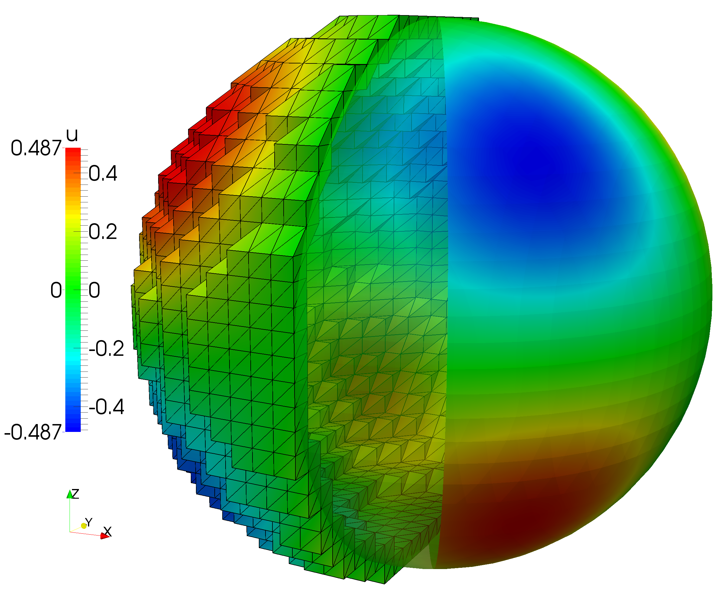
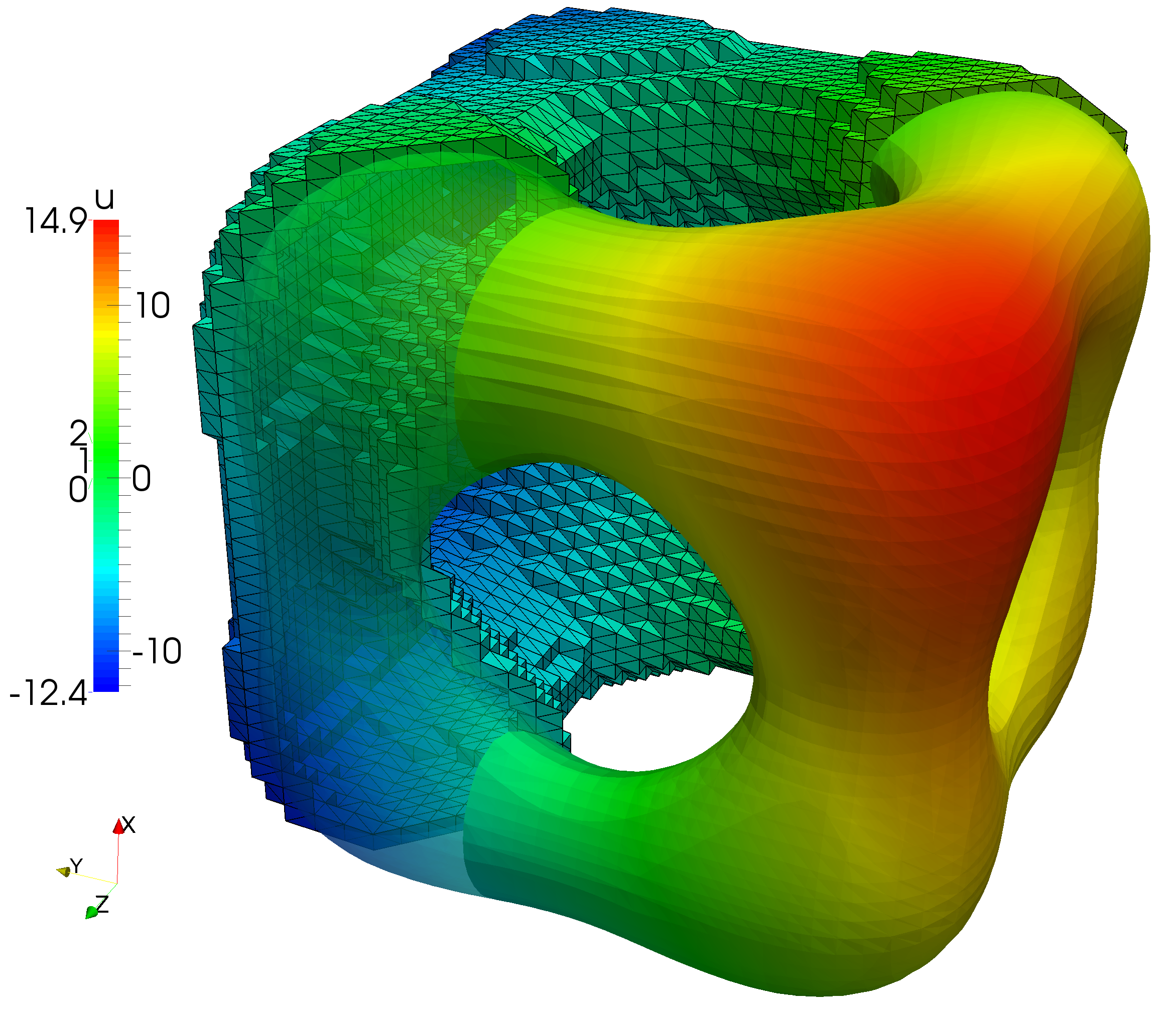
Figure 2. Computed solutions for example 1 (left) and example 2 (right). The left part of each solution plot shows the approximation $u_{h}$ as computed on the active mesh $\mathcal{T}_{h}$ while the right part displays $u_{h}$ restricted to the surface mesh $\mathcal{K}_{h}$.

Level $k$	$\|u_{k}-u\|_{H^{1}(\Gamma_{h})}$		EOC	$\|u_{k}-u\|_{L^{2}(\Gamma_{h})}$		EOC	$\|u_{k}-u\|_{L^{\infty}(N_{h})}$		EOC
$0$	$1.27$	$\cdot 10^{0}$	–	$2.49$	$\cdot 10^{-1}$	–	$1.44$	$\cdot 10^{-1}$	–
$1$	$6.87$	$\cdot 10^{-1}$	$0.89$	$7.28$	$\cdot 10^{-2}$	$1.78$	$5.10$	$\cdot 10^{-2}$	$1.50$
$2$	$3.73$	$\cdot 10^{-1}$	$0.88$	$1.93$	$\cdot 10^{-2}$	$1.91$	$1.35$	$\cdot 10^{-2}$	$1.92$
$3$	$1.74$	$\cdot 10^{-1}$	$1.10$	$4.81$	$\cdot 10^{-3}$	$2.01$	$3.70$	$\cdot 10^{-3}$	$1.86$
$4$	$8.65$	$\cdot 10^{-2}$	$1.01$	$1.20$	$\cdot 10^{-3}$	$2.01$	$9.42$	$\cdot 10^{-4}$	$1.97$
$5$	$4.34$	$\cdot 10^{-2}$	$0.99$	$3.01$	$\cdot 10^{-4}$	$1.99$	$2.39$	$\cdot 10^{-4}$	$1.98$

Table 1. Convergence rates for example 1 with $\beta_{E}=\beta_{F}=50$ and $\gamma=0.01$.

Level $k$	$\|u_{k}-u\|_{H^{1}(\Gamma_{h})}$		EOC	$\|u_{k}-u\|_{L^{2}(\Gamma_{h})}$		EOC	$\|u_{k}-u\|_{L^{\infty}(N_{h})}$		EOC
$0$	$2.21$	$\cdot 10^{1}$	–	$1.48$	$\cdot 10^{1}$	–	$4.56$	$\cdot 10^{0}$	–
$1$	$7.33$	$\cdot 10^{0}$	$1.59$	$1.84$	$\cdot 10^{0}$	$3.01$	$8.54$	$\cdot 10^{-1}$	$2.42$
$2$	$3.12$	$\cdot 10^{0}$	$1.23$	$5.41$	$\cdot 10^{-1}$	$1.77$	$2.26$	$\cdot 10^{-1}$	$1.92$
$3$	$1.61$	$\cdot 10^{0}$	$0.95$	$1.16$	$\cdot 10^{-1}$	$2.22$	$5.38$	$\cdot 10^{-2}$	$2.07$
$4$	$7.65$	$\cdot 10^{-1}$	$1.07$	$2.86$	$\cdot 10^{-2}$	$2.02$	$1.28$	$\cdot 10^{-2}$	$2.07$
$5$	$3.78$	$\cdot 10^{-1}$	$1.02$	$7.18$	$\cdot 10^{-3}$	$2.00$	$3.32$	$\cdot 10^{-3}$	$1.95$

Level $k$	$\|u_{k}-u\|_{H^{1}(\Gamma_{h})}$		EOC	$\|u_{k}-u\|_{L^{2}(\Gamma_{h})}$		EOC	$\|u_{k}-u\|_{L^{\infty}(N_{h})}$		EOC
$0$	$2.20$	$\cdot 10^{1}$	–	$1.49$	$\cdot 10^{1}$	–	$4.59$	$\cdot 10^{0}$	–
$1$	$7.22$	$\cdot 10^{0}$	$1.61$	$1.80$	$\cdot 10^{0}$	$3.05$	$8.20$	$\cdot 10^{-1}$	$2.48$
$2$	$3.09$	$\cdot 10^{0}$	$1.22$	$5.38$	$\cdot 10^{-1}$	$1.74$	$2.23$	$\cdot 10^{-1}$	$1.88$
$3$	$1.62$	$\cdot 10^{0}$	$0.93$	$1.16$	$\cdot 10^{-1}$	$2.22$	$5.27$	$\cdot 10^{-2}$	$2.08$
$4$	$7.64$	$\cdot 10^{-1}$	$1.09$	$2.85$	$\cdot 10^{-2}$	$2.02$	$1.25$	$\cdot 10^{-2}$	$2.07$
$5$	$3.78$	$\cdot 10^{-1}$	$1.02$	$7.14$	$\cdot 10^{-3}$	$2.00$	$3.29$	$\cdot 10^{-3}$	$1.93$

Table 2. Convergence rates for example 2 with $\beta_{E}=\beta_{F}=50$ (top) and $\beta_{E}=0$, $\beta_{F}=500$ (bottom) and $\gamma=0.01$ in both cases.

8.2. Condition Number Tests

Finally, we numerically examine the mesh-size dependency of the condition number of our proposed method and study how the positioning of the surface in the background mesh affects the condition number.

Let $\{\mathcal{T}_{k}\}_{k=0}^{3}$ be a sequence of successively refined tessellations of $\Omega=[-1.6,1.6]^{3}$ with mesh size $h=3.2/5\cdot 2^{-k}$. On each refinement level $k$, we generate a family of surfaces $\{\Gamma_{\delta}\}_{0\leqslant\delta\leqslant 1}$ by translating the unit-sphere $S^{2}=\{x\in\mathbb{R}^{3}:\|x\|=1\}$ along the diagonal $(h,h,h)$; that is, $\Gamma_{\delta}=S^{2}+\delta_{0}(h,h,h)$ with $\delta\in[0,1]$. For $\delta=l/500$, $l=0,\ldots,500$, we compute the condition number $\kappa_{\delta}(\mathcal{A})$ as the ratio of the absolute value of the largest (in modulus) and smallest (in modulus), non-zero eigenvalue. For each refinement level $k$, the resulting condition numbers are plotted in Figure 3 as a function of $\delta$. We observe that the position of $\Gamma$ relative to the background mesh $\mathcal{T}_{k}$ has very little effect on the condition number when the stabilization parameters $\beta_{F}$ and $\gamma$ are chosen sufficiently large. In contrast, the condition number is highly sensitive and clearly unbounded as a function of $\delta$ if we set either penalty parameter in (2.26) to $0$ as the corresponding plots in Figure 3 reveal. Finally, scaling the largest computed condition number on each refinement level $k$ with $k^{-2}$ confirms the theoretically proven $O(h^{-2})$ bound, see Table 3.

To further elucidate the importance of the various stabilization terms in (2.26), we conduct a second numerical experiment inspired by the results presented in Olshanskii and Reusken [31]. Olshanskii and Reusken [31] show that diagonal preconditioning yields robust condition number bounds and cures the discrete system from being severely ill-conditioned when a continuous piecewise linear ansatz space is used, see also Figure 3. Thus, no stabilization is needed and $\gamma$, as the only relevant penalty parameter in the continuous case, can be set to $0$. Repeating the same experiment for our proposed cut discontinuous Galerkin method with either penalty parameter $\beta_{F}$ or $\gamma$ deactivated shows that the same conclusion is not true if discontinuous finite element functions are employed. The reason lies in the construction of the approximation space by restricting the finite element space defined on the background mesh to the surface. For each element $T\in\mathcal{T}_{h}$, restricting the shape functions defined on $T$ to the surface part $K=\Gamma_{h}\cap T$ clearly yields a set of locally linearly dependent functions on $K$. With the basis functions stretching over several elements, this effect is usually counteracted in the case of continuous finite element functions, since curvature effects lead to different linear dependencies on each element. Thus the resulting set of finite element functions on $\mathcal{K}_{h}$ is usually only “nearly” linearly dependent and therefore a well-conditioned system can be obtained by means of proper preconditioning. However, in the discontinuous case, restricting the finite element basis on $\mathcal{T}_{h}$ to the surface produces a globally linearly dependent set of discrete functions, even in the presence of highly curved surfaces, as interelement continuity is imposed only weakly via (2.26). We also observe that if we enforce nearly inter-element continuity of the discrete functions by choosing a very large penalty parameter, e.g., $\beta_{F}=5e6$, diagonal preconditioning yields robust, albeit large, bounds for the condition number, see Figure 3.

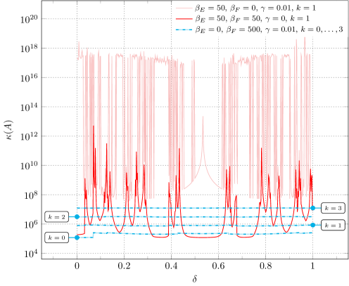
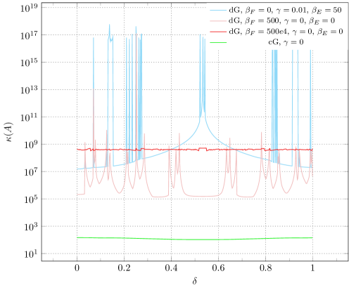
Figure 3. Condition numbers plotted as a function of the position parameter $\delta$. Top: With either $\beta_{F}=0$ or $\gamma=0$, the condition number is highly sensitive to the surface positioning in the background mesh. With both penalties activated, the condition number is robust and the edge-based penalty term $\beta_{E}$ can be omitted. Bottom: Diagonally preconditioned surface CutFEMs. For an unstabilized continuous Galerkin (cG) method, preconditioning gives robust condition numbers while for our discontinuous CutFEM (dG), the preconditioned system is still highly dependent on the surface position if either $\beta_{F}=0$ and $\gamma=0$.

$k$	1	2	3	4
$k^{-2}\max_{\delta}\{\kappa_{\delta}(\mathcal{A})\}$	7370.36	7167.30	7205.85	6271.44

Table 3. Maximum of scaled condition numbers for each refinement level $k$.

References

- Brenner [2003] S. C. Brenner. Poincaré–Friedrichs inequalities for piecewise functions. SIAM J. Numer. Anal., 41(1):306–324, 2003.
- Burman and Hansbo [2012] E. Burman and P. Hansbo. Fictitious domain finite element methods using cut elements: II. A stabilized Nitsche method. Appl. Numer. Math., 62(4), 2012.
- Burman and Hansbo [2013] E. Burman and P. Hansbo. Fictitious domain methods using cut elements: III. A stabilized Nitsche method for Stokes’ problem. ESAIM, Math. Model. Num. Anal., page 19, 2013.
- Burman et al. [2006] E. Burman, M.A. Fernández, and P. Hansbo. Continuous interior penalty finite element method for Oseen’s equations. SIAM J. Numer. Anal., 44(3):1248–1274, 2006.
- Burman et al. [2015a] E. Burman, S. Claus, P. Hansbo, M.G. Larson, and A. Massing. Cutfem: discretizing geometry and partial differential equations. Internat. J. Numer. Meth. Engng, 2015a. doi: 10.1002/nme.4823.
- Burman et al. [2015b] E. Burman, P. Hansbo, and M. G. Larson. A stabilized cut finite element method for partial differential equations on surfaces: The Laplace–Beltrami operator. Comput. Methods Appl. Mech. Engrg., 285:188–207, 2015b.
- Burman et al. [2015c] E. Burman, P. Hansbo, M. G. Larson, and S. Zahedi. Stabilized cut finite element methods for convection problems on surfaces. In preparation, 2015c.
- Burman et al. [2015d] E. Burman, P. Hansbo, M.G. Larson, and S. Zahedi. Cut finite element methods for coupled bulk-surface problems. Numer. Math., 2015d. doi: 10.1007/s00211-015-0744-3.
- Chernyshenko and Olshanskii [2015] A. Y. Chernyshenko and M. A. Olshanskii. An adaptive octree finite element method for PDEs posed on surfaces. Comput. Methods Appl. Mech. Engrg., 291:146–172, August 2015.
- Deckelnick et al. [2014] K. Deckelnick, C. M. Elliott, and T. Ranner. Unfitted finite element methods using bulk meshes for surface partial differential equations. SIAM J. Numer. Anal., 52(4):2137–2162, 2014.
- Dedner et al. [2013] A. Dedner, P. Madhavan, and B. Stinner. Analysis of the discontinuous Galerkin method for elliptic problems on surfaces. IMA J. Numer. Anal., 33(3):952–973, 2013.
- Demlow and Olshanskii [2012] A. Demlow and M. A. A Olshanskii. An adaptive surface finite element method based on volume meshes. SIAM J. Numer. Anal., 50(3):1624–1647, 2012.
- Dziuk [1988] G. Dziuk. Finite elements for the Beltrami operator on arbitrary surfaces. In Partial differential equations and calculus of variations, volume 1357 of Lecture Notes in Math., pages 142–155. Springer, Berlin, 1988.
- Dziuk and Elliott [2013] G. Dziuk and C. M. Elliott. Finite element methods for surface PDEs. Acta Numer., 22:289–396, 2013.
- Ern and Guermond [2006] A. Ern and J. L. Guermond. Evaluation of the condition number in linear systems arising in finite element approximations. ESAIM: Math. Model. Num. Anal., 40(1):29–48, 2006.
- Evans and Gariepy [1992] L. C. Evans and R. F. Gariepy. Measure Theory and Fine Properties of Functions. Studies in Advanced Mathematics. CRC Press, Boca Raton, FL, 1992.
- Giesselmann and Müller [2014] J. Giesselmann and T. Müller. Geometric error of finite volume schemes for conservation laws on evolving surfaces. Numer. Math., 128(3):489–516, 2014.
- Gilbarg and Trudinger [2001] D. Gilbarg and N. S. Trudinger. Elliptic Partial Differential Equations of Second Order. Classics in Mathematics. Springer-Verlag, Berlin, 2001.
- Grande and Reusken [2014] J. Grande and A. Reusken. A higher-order finite element method for partial differential equations on surfaces. Preprint 401, IGPM, RWTH Aachen University., 2014.
- Gross et al. [2015] S. Gross, M. A. Olshanskii, and A. Reusken. A trace finite element method for a class of coupled bulk-interface transport problems. ESAIM: Math. Model. Numer. Anal., 2015. doi: 10.1051/m2an/2015013.
- Groß and Reusken [2007] Sven Groß and Arnold Reusken. An extended pressure finite element space for two-phase incompressible flows with surface tension. J. Comput. Phys., 224(1):40–58, 2007.
- Hansbo and Hansbo [2002] A. Hansbo and P. Hansbo. An unfitted finite element method, based on Nitsche’s method, for elliptic interface problems. Comput. Methods Appl. Mech. Engrg., 191(47-48):5537–5552, 2002.
- Hansbo et al. [2003] A. Hansbo, P. Hansbo, and Mats G. Larson. A finite element method on composite grids based on Nitsche’s method. ESAIM: Math. Model. Num. Anal., 37(3):495–514, 2003.
- Hansbo et al. [2014] P. Hansbo, M. G. Larson, and S. Zahedi. A cut finite element method for a Stokes interface problem. Appl. Numer. Math., 85:90–114, 2014.
- Hansbo et al. [2015] P. Hansbo, M. G. Larson, and S. Zahedi. Characteristic cut finite element methods for convection–diffusion problems on time dependent surfaces. Comput. Methods Appl. Mech. Engrg., 293:431–461, 2015.
- Heimann et al. [2013] F. Heimann, C. Engwer, O. Ippisch, and P. Bastian. An unfitted interior penalty discontinuous Galerkin method for incompressible Navier–Stokes two–phase flow. Internat. J. Numer. Methods Fluids, 71(3):269–293, 2013.
- Johansson and Larson [2013] A. Johansson and M.G. Larson. A high order discontinuous Galerkin Nitsche method for elliptic problems with fictitious boundary. Numer. Math., 123(4), 2013.
- Massing et al. [2013] A. Massing, M.G. Larson, and A. Logg. Efficient implementation of finite element methods on non-matching and overlapping meshes in 3d. SIAM J. Sci. Comput., 35(1):C23–C47, 2013.
- Massing et al. [2014a] A. Massing, M. G. Larson, A. Logg, and M. E. Rognes. A stabilized Nitsche overlapping mesh method for the Stokes problem. Numer. Math., 128(1):73–101, 2014a.
- Massing et al. [2014b] A. Massing, M.G. Larson, A. Logg, and M.E. Rognes. A stabilized Nitsche fictitious domain method for the Stokes problem. J. Sci. Comput., 61(3):604–628, 2014b. doi: 10.1007/s10915-014-9838-9.
- Olshanskii and Reusken [2010] M. A. Olshanskii and A. Reusken. A finite element method for surface PDEs: matrix properties. Numer. Math., 114(3):491–520, 2010.
- Olshanskii et al. [2009] M. A. Olshanskii, A. Reusken, and J. Grande. A finite element method for elliptic equations on surfaces. SIAM J. Numer. Anal., 47(5):3339–3358, 2009.
- Olshanskii et al. [2014a] M. A. Olshanskii, A. Reusken, and X. Xu. A stabilized finite element method for advection–diffusion equations on surfaces. IMA J. Numer. Anal., 34(2):732–758, 2014a.
- Olshanskii et al. [2014b] M. A. Olshanskii, A. Reusken, and X. Xu. An Eulerian space-time finite element method for diffusion problems on evolving surfaces. SIAM J. Numer. Anal., 52(3):1354–1377, 2014b.
- Scott and Zhang [1990] R. Scott and S. Zhang. Finite element interpolation of nonsmooth functions satisfying boundary conditions. Math. Comp., 54(190):483–493, 1990.
- Sollie et al. [2011] W. E. H. Sollie, O. Bokhove, and J. J. W. van der Vegt. Space–time discontinuous Galerkin finite element method for two-fluid flows. J. Comput. Phys., 230(3):789–817, 2011.
- Wang and Chen [2015] Qiuliang Wang and Jinru Chen. A new unfitted stabilized Nitsche’s finite element method for Stokes interface problems. Comput. Math. Appl., 2015.