Abstract

We compute the pion quark Generalised Parton Distribution H and quark Double Distributions in a coupled Bethe-Salpeter and Dyson-Schwinger approach in terms of quark flavors or isospin states. We use analytic expressions inspired by the numerical resolution of Dyson-Schwinger and Bethe-Salpeter equations. We obtain an analytic expression for the pion Generalised Parton Distribution at a low scale. Our model fulfils most of the required symmetry properties and compares very well to experimental pion form factor or valence parton distribution function experimental data. In addition, we have highlighted limitations of the so-called impulse approximation, which breaks symmetries when computing the valence parton distribution function. Doing so, we introduced new terms which were neglected before. Finally, we also shed light on a specific property of the pion GPD: Polyakov soft pion theorem.

1 Introduction

Generalised Parton Distributions (GPDs) were introduced in the 1990 [1, 2, 3] and since then have been deeply studied both theoretically (see e.g. the reviews [4, 5, 6]) and experimentally. New results from Jefferson Laboratory facilities (JLab) on Deep-Virtual Compton Scattering (DVCS) on a proton target have recently been presented [7, 8]. Several phenomenological parametrisations have been developed in order to fit the proton GPDs [9, 10, 11, 12, 13, 14]. Yet until now, none of them has been fully derived from QCD dynamics only.

In order to generate the parton structure of hadron in a dynamical way, one can turn to the Dyson-Schwinger (DS) and Bethe-Salpeter (BS) equations. Those equations are coupled and can be solved using specific truncation schemes. In the following, we focus on the pion GPD, which is simpler to compute in the present framework than the proton one. The pion GPD inspired many theoretical studies [15, 16, 17, 18, 19, 20] in spite of the restricted set of existing experimental data, related to the valence Parton Distribution Function (PDF) [21] and the form factors [22, 23]. Our approach to the pion GPD is detailed in the first section. The second section deals with the restoration of the symmetry under the exchange $x\leftrightarrow 1-x$ in the forward case.

2 GPD Computations

The pion quark GPD $H^{q}(x,\xi,t)$ is formally defined as:

$$H(x,\xi,t)=\frac{1}{2}\int\frac{\textrm{d}z^{-}}{2\pi}\,e^{ixP^{+}z^{-}}\left\langle P+\frac{\Delta}{2}\left|\bar{q}\left(-\frac{z}{2}\right)\gamma^{+}q\left(\frac{z}{2}\right)\right|P-\frac{\Delta}{2}\right\rangle_{z^{+}=0,z_{\perp}=0},$$ (1)

where $t=\Delta^{2}$ and $\xi=-\frac{\Delta^{+}}{2P^{+}}$. In our approach [24, 25], we define the pion GPD by the set of its Mellin moments $\mathcal{M}_{n}(\xi,t)$:

$$\mathcal{M}_{n}(\xi,t)=\int\textrm{d}x~{}x^{n}H(x,\xi,t).$$ (2)

These moments are computed in the triangle diagram approximation illustrated on figure 1.

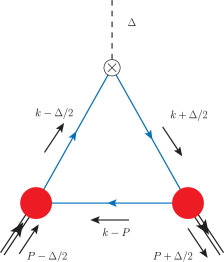
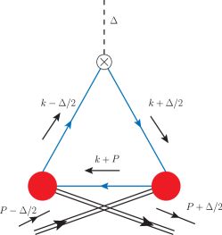
Figure 1: Mellin moments computed in the triangle approximation for the pion valence dressed quarks. Left panel: quark case. Right Panel: anti-quark case.

Consequently, the inserted operators, depicted on figure 1 by a cross, are the local twist-two quark operators arising from the operator product expansion. They can be computed as:

$$2(P\cdot n)^{m+1}\mathcal{M}_{m}(\xi,t) = \textrm{Tr}\int\frac{\mathrm{d}^{4}k}{(2\pi)^{4}}\,(k\cdot n)^{m}i\Gamma_{\pi}(k-\frac{\Delta}{2},P-\frac{\Delta}{2})~{}S(k-\frac{\Delta}{2})$$ (3)

$$i\gamma\cdot n~{}S(k+\frac{\Delta}{2})~{}i\bar{\Gamma}_{\pi}(k+\frac{\Delta}{2},P+\frac{\Delta}{2})~{}S(k-P),$$

where the Bethe-Salpeter vertices $\Gamma_{\pi}$ and propagator $S$ are taken as:

$$S(p) = \big{[}-i\gamma\cdot p+M\big{]}\Delta_{M}(p^{2}),$$ (4)

$$\Delta_{M}(s) = \frac{1}{s+M^{2}},$$ (5)

$$\Gamma_{\pi}(k,p) = i\gamma_{5}\frac{M}{f_{\pi}}M^{2\nu}\int_{-1}^{+1}\mathrm{d}z\,\rho_{\nu}(z)\ \left[\Delta_{M}(k_{+z}^{2})\right]^{\nu};$$ (6)

$$\rho_{\nu}(z) = R_{\nu}(1-z^{2})^{\nu}.$$ (7)

These functional forms have been introduced in Ref. [26] and allow one to fit the numerical solutions of the Dyson-Schwinger and Bethe-Salpeter equations. Here we will fit a single free parameter, $M$, the second one, $\nu$, being fixed to 1. This value of $\nu$ is the one giving back the pion asymptotic Distribution Amplitude (DA). From that point, the GPD can be analytically reconstruct from its Mellin using the so-called Double Distributions (DDs). Indeed, performing the computation, it is possible to identify the two DDs $F^{q}(\beta,\alpha,t)$ and $G^{q}(\beta,\alpha,t)$ which are related to the pion GPD through the Radon transform:

$$H_{\pi}^{q}(x,\xi,t)=\int_{-1}^{1}\textrm{d}\beta\int^{1-|\beta|}_{-1+|\beta|}\textrm{d}\alpha\Big{(}F^{q}(\beta,\alpha,t)+G^{q}(\beta,\alpha,t)\Big{)}\delta(x-\beta-\xi\alpha).$$ (8)

It is then possible to get an algebraic formula for the GPD. The result is plotted on figure 2.

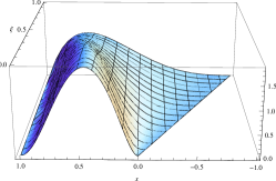
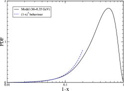
Figure 2: Left Panel: reconstruction of the GPD when $t\rightarrow 0$. Support and continuity properties are well illustrated on this plot. Right Panel: PDF large-$x$ behaviour, which fits the one predicted in the pertubative case.

Being able to compute algebraically the GPD provides us a significant advantage to check the different intrinsic properties that the model should respect. Due to the property of the algebraic DDs identified from our calculations, it is possible to conclude that the support property of the valence GPD, the continuity on the lines $x=\pm\xi$ and the parity in $\xi$ are fulfilled by our GPD model. Moreover, the DD formalism ensure the polynomiality property by construction. Finally, one can check that the resulting PDF gets the same large-$x$ behaviour than the one predicted by perturbation theory.

3 Soft Pion theorem

In Ref. [27], it has been shown that, it was possible to relate the pion DA to the pion GPD. In the kinematic limit when $t\rightarrow 0$ and $\xi\rightarrow 1$, one actually gets:

$$H^{u}(x,1,0)=\frac{1}{2}\varphi_{\pi}\left(\frac{1+x}{2}\right),$$ (9)

where $\varphi_{\pi}$ is the pion DA. The algebraic model coming from equations (4)-(7) have been developed in order to describe $\varphi_{\pi}$. And indeed, when computed in Ref. [26], it leads to the asymptotic pion DA. Therefore, one could expect that, due to the soft pion theorem, when $\xi$ goes to $1$ and $t$ vanishes, the algebraic GPD model tend to the pion asymptotic DA. It is not the case due to a specific feature of the algebraic model. Indeed, working only with the building blocks of the solution of the DS-BS equations leads to a violation of the Axial-Vector Ward-Takashi identity (AVWTI), which gives in the chiral limit:

$$P^{\mu}\Gamma_{5\mu}^{i}(k,P)=\frac{\tau^{i}}{2}\left(S^{-1}(k-\frac{P}{2})i\gamma_{5}+i\gamma_{5}S^{-1}(k+\frac{P}{2})\right),$$ (10)

where $P$ is the total momentum entering the axial-vector vertex, $k$ the relative one, and the $\tau^{i}$ the Pauli matrices. When computed consistently in the rainbow ladder truncation scheme, the full solution of the DS-BS equation fulfils the AVWTI. Therefore, inserting the reduction formula:

$$2f_{\pi}\Gamma_{\pi}(k;p) \stackrel{{\scriptstyle p\simeq 0}}{{\propto}} p^{\mu}\Gamma_{5\mu}(k,p)\,,$$ (11)

$$2r_{\pi}\Gamma_{\pi}(k;p) \stackrel{{\scriptstyle p^{2}\simeq 0}}{{\propto}} p^{2}\Gamma_{5}(k,p)\,,$$ (12)

allows one to write the triangle diagram in terms of axial-vector and pseudo-scalar vertices. Then, as shown in Ref. [28], most of the gluon ladders coming from the insertion of the AVWTI compensate each others, leading to the pion DA. Consequently, in the rainbow ladder truncation scheme, the soft pion theorem is automatically fulfilled providing that the Dyson-Schwinger and Bethe-Salpeter equations are solved consistently with the AVWTI.

4 Additionnal contributions

If it is possible to recover the soft pion theorem through a triangle diagram computation, such an approximation still has its own limitations. Focusing on the forward limit (i.e. $t=0$ and $\xi=0$), the PDF $q_{\pi}^{\textrm{Tr}}(x)$ can be written as:

$$q_{\pi}^{\textrm{Tr}}(x)=\frac{72}{25}\Big{(}(30-15x+8x^{2}-2x^{3})x^{3}\log x +(3+2x^{2})(1-x)^{4}\log(1-x)$$ (13)

$$+(3+15x+5x^{2}-2x^{3})x(1-x)\Big{)}.$$

If this PDF is in agreement with the pertubative prediction at large $x$, it suffers a significant drawback, as it is not symmetric with respect to the $x\leftrightarrow 1-x$ exchange. The small asymmetry is due to the fact that contributions have been neglected, due to the triangle approximation. Indeed, it has been shown in Ref. [29], that one has to add new terms in order to fulfil the $x\leftrightarrow 1-x$ symmetry:

$$\vbox{\hbox{\includegraphics[width=65.04034pt]{MellinMomentsGPD.eps}}}\simeq\vbox{\hbox{\includegraphics[width=65.04034pt]{MellinMomentsTriangle.eps}}}+\vbox{\hbox{\includegraphics[width=65.04034pt]{MellinMomentsAdditional1.eps}}}+\vbox{\hbox{\includegraphics[width=65.04034pt]{MellinMomentsAdditional2.eps}}},$$ (14)

where:

$$\vbox{\hbox{\includegraphics[width=86.72267pt]{SquareVertex.eps}}}=-\frac{1}{2}(k\cdot n)^{m}n^{\mu}\frac{\partial\Gamma_{\pi}^{q}}{\partial k^{\mu}}\left(k,P\right).$$ (15)

It is then possible to compute and additional component to the PDF $q_{\pi}^{\textrm{ad}}(x)$:

$$q_{\pi}^{\textrm{ad}}(x)=\frac{72}{25}\Bigg{(}-\left(2x^{3}+4x+9\right)(x-1)^{3}\log(1-x) +x^{3}(2x((x-3)x+5)-15)\log(x)$$

$$-x(x-1)(2x-1)((x-1)x-9)\Bigg{)}.$$ (16)

Then summing the different contributions, one gets the total PDF $q_{\pi}^{\textrm{tot}}(x)$:

$$q_{\pi}^{\textrm{tot}}(x) = q_{\pi}^{\textrm{Tr}}(x)+q_{\pi}^{\textrm{ad}}(x)$$ (17)

$$= \frac{72}{25}\Bigg{(}x^{3}(x(2x-5)+15)\log(x)-\left(2x^{2}+x+12\right)(x-1)^{3}\log(1-x)$$

$$-2x(x-1)((x-1)x+6)\Bigg{)},$$

which fulfils the $x\leftrightarrow 1-x$ symmetry as shown on figure 3.This analysis has also led to a new GPD Ansatz described in Ref. [28, 30].

Figure 3: Contributions to the PDF and their sum.

5 Conclusion

We have developed a new GPD model. It is based on algebraic building blocks of solutions of the Dyson-Schwinger and Bethe-Salpeter equations. Within this procedure, our model fulfils most of the required theoretical constraints. In addition, our model is in good agreement with available experimental data. Computations has been done analytically up to the end, allowing one to identify limitations of the triangle diagram approximation, and thus to improve it. We have also emphasised the key-role of the AVWTI in the realisation of the soft pion theorem. Future models of pion GPDs will therefore have to deal with those additional constraints.

6 Acknowledgement

I thank my collaborators L. Chang, H. Moutarde, C.D. Roberts, J. Rodriguez-Quintero, F. Sabatié and P.C. Tandy with whom this work has been done. I also thank A. Besse, P. Fromholz, P. Kroll, J-Ph. Landsberg, C. Lorcé, B. Pire and S. Wallon for valuable discussions. This work is partly supported by the Commissariat à l’Energie Atomique, the Joint Research Activity ”Study of Strongly Interacting Matter” (acronym HadronPhysics3, Grant Agreement n.283286) under the Seventh Framework Programme of the European Community, by the GDR 3034 PH-QCD ”Chromodynamique Quantique et Physique des Hadrons”, the ANR-12-MONU-0008-01 ”PARTONS”.

References

- [1] Dieter Mueller, D. Robaschik, B. Geyer, F.M. Dittes, and J. Hořeǰsi. Wave functions, evolution equations and evolution kernels from light ray operators of QCD. Fortsch.Phys., 42:101–141, 1994, hep-ph/9812448.
- [2] Xiang-Dong Ji. Deeply virtual Compton scattering. Phys.Rev., D55:7114–7125, 1997, hep-ph/9609381.
- [3] A.V. Radyushkin. Nonforward parton distributions. Phys.Rev., D56:5524–5557, 1997, hep-ph/9704207.
- [4] M. Diehl. Generalized parton distributions. Phys.Rept., 388:41–277, 2003, hep-ph/0307382.
- [5] A.V. Belitsky and A.V. Radyushkin. Unraveling hadron structure with generalized parton distributions. Phys.Rept., 418:1–387, 2005, hep-ph/0504030.
- [6] Michel Guidal, Hervé Moutarde, and Marc Vanderhaeghen. Generalized Parton Distributions in the valence region from Deeply Virtual Compton Scattering. Rept.Prog.Phys., 76:066202, 2013, 1303.6600.
- [7] M. Defurne, M. Amaryan, K.A. Aniol, M. Beaumel, H. Benaoum, et al. The E00-110 experiment in Jefferson Lab’s Hall A: Deeply Virtual Compton Scattering off the Proton at 6 GeV. 2015, 1504.05453.
- [8] H.S. Jo et al. Cross sections for the exclusive photon electroproduction on the proton and Generalized Parton Distributions. 2015, 1504.02009.
- [9] S.V. Goloskokov and P. Kroll. Vector meson electroproduction at small Bjorken-x and generalized parton distributions. Eur.Phys.J., C42:281–301, 2005, hep-ph/0501242.
- [10] M. Guidal, M.V. Polyakov, A.V. Radyushkin, and M. Vanderhaeghen. Nucleon form-factors from generalized parton distributions. Phys.Rev., D72:054013, 2005, hep-ph/0410251.
- [11] Kresimir Kumerički and Dieter Mueller. Deeply virtual Compton scattering at small and the access to the GPD H. Nucl.Phys., B841:1–58, 2010, 0904.0458.
- [12] C. Mezrag, H. Moutarde, and F. Sabatié. Test of two new parameterizations of the Generalized Parton Distribution . Phys.Rev., D88:014001, 2013, 1304.7645.
- [13] Maxim V. Polyakov and Marc Vanderhaeghen. Taming Deeply Virtual Compton Scattering. 2008, 0803.1271.
- [14] Gary R. Goldstein, J. Osvaldo Gonzalez Hernandez, and Simonetta Liuti. Flexible Parametrization of Generalized Parton Distributions from Deeply Virtual Compton Scattering Observables. Phys.Rev., D84:034007, 2011, 1012.3776.
- [15] B.C. Tiburzi and G.A. Miller. Generalized parton distributions and double distributions for q anti-q pions. Phys.Rev., D67:113004, 2003, hep-ph/0212238.
- [16] L. Theussl, S. Noguera, and V. Vento. Generalized parton distributions of the pion in a Bethe-Salpeter approach. Eur.Phys.J., A20:483–498, 2004, nucl-th/0211036.
- [17] F. Bissey, J.R. Cudell, J. Cugnon, J.P. Lansberg, and P. Stassart. A Model for the off forward structure functions of the pion. Phys.Lett., B587:189–200, 2004, hep-ph/0310184.
- [18] A. Van Dyck, T. Van Cauteren, and Jan Ryckebusch. Support of generalized parton distributions in Bethe-Salpeter models of hadrons. Phys.Lett., B662:413–416, 2008, 0710.2271.
- [19] T. Frederico, E. Pace, B. Pasquini, and G. Salme. Pion Generalized Parton Distributions with covariant and Light-front constituent quark models. Phys.Rev., D80:054021, 2009, 0907.5566.
- [20] Alexander E. Dorokhov, Wojciech Broniowski, and Enrique Ruiz Arriola. Generalized Quark Transversity Distribution of the Pion in Chiral Quark Models. Phys.Rev., D84:074015, 2011, 1107.5631.
- [21] Matthias Aicher, Andreas Schafer, and Werner Vogelsang. Soft-gluon resummation and the valence parton distribution function of the pion. Phys.Rev.Lett., 105:252003, 2010, 1009.2481.
- [22] S.R. Amendolia et al. A Measurement of the Space - Like Pion Electromagnetic Form-Factor. Nucl.Phys., B277:168, 1986.
- [23] G.M. Huber et al. Charged pion form-factor between Q**2 = 0.60-GeV**2 and 2.45-GeV**2. II. Determination of, and results for, the pion form-factor. Phys.Rev., C78:045203, 2008, 0809.3052.
- [24] C. Mezrag, H. Moutarde, J. Rodríguez-Quintero, and F. Sabatié. Towards a Pion Generalized Parton Distribution Model from Dyson-Schwinger Equations. 2014, 1406.7425.
- [25] C. Mezrag. Modeling the pion Generalized Parton Distribution. 2015, 1501.03699.
- [26] Lei Chang, I.C. Cloet, J.J. Cobos-Martinez, C.D. Roberts, S.M. Schmidt, et al. Imaging dynamical chiral symmetry breaking: pion wave function on the light front. Phys.Rev.Lett., 110:132001, 2013, 1301.0324.
- [27] Maxim V. Polyakov. Hard exclusive electroproduction of two pions and their resonances. Nucl.Phys., B555:231, 1999, hep-ph/9809483.
- [28] C. Mezrag, L. Chang, H. Moutarde, C.D. Roberts, J. Rodríguez-Quintero, et al. Sketching the pion’s valence-quark generalised parton distribution. Phys.Lett., B741:190–196, 2014, 1411.6634.
- [29] Lei Chang, Cédric Mezrag, Hervé Moutarde, Craig D. Roberts, Jose Rodriguez-Quintero, et al. Basic features of the pion valence-quark distribution function. Phys.Lett., B737:23–29, 2014, 1406.5450.
- [30] L. Chang, C. Mezrag, H. Moutarde, C.D. Roberts, J. Rodríguez-Quintero, et al. DSE inspired model for the pion’s valence dressed-quark GPD. 2015, 1503.08645.