Solar neutrinos and neutrino physics

Abstract

Solar neutrino studies triggered and largely motivated the major developments in neutrino physics in the last 50 years. Theory of neutrino propagation in different media with matter and fields has been elaborated. It includes oscillations in vacuum and matter, resonance flavor conversion and resonance oscillations, spin and spin-flavor precession, etc. LMA MSW has been established as the true solution of the solar neutrino problem. Parameters $\theta_{12}$ and $\Delta m^{2}_{21}$ have been measured; $\theta_{13}$ extracted from the solar data is in agreement with results from reactor experiments. Solar neutrino studies provide a sensitive way to test theory of neutrino oscillations and conversion. Characterized by long baseline, huge fluxes and low energies they are a powerful set-up to search for new physics beyond the standard $3\nu$ paradigm: new neutrino states, sterile neutrinos, non-standard neutrino interactions, effects of violation of fundamental symmetries, new dynamics of neutrino propagation, probes of space and time. These searches allow us to get stringent, and in some cases unique bounds on new physics. We summarize the results on physics of propagation, neutrino properties and physics beyond the standard model obtained from studies of solar neutrinos.

1 Introduction

“If the oscillation length is large… from the point of view of detection possibilities an ideal object is the Sun.” This statement from Pontecorvo’s 1967 paper Pontecorvo:1967fh published before release of the first Homestake experiment results Davis:1968cp can be considered as the starting point for the solar neutrino studies of new physics.

Observation of the deficit of signal in the Homestake experiment was the first indication of existence of oscillations. This result had triggered vast experimental chapt3 and theoretical developments in neutrino physics. On theoretical side, various non-standard properties of neutrinos have been introduced and new effects in propagation of neutrinos have been proposed. These include:

1. Neutrino spin-precession in the magnetic fields of the Sun due to large magnetic moments of neutrinos Cisneros:1970nq ; Okun:1986na : electromagnetic properties of neutrinos have been studied in details.

2. Neutrino decays: Among various possibilities (radiative, $3\nu$ decay, etc.) the decay into light scalar, e.g., Majoron, is less restricted Bahcall:1972my ; Berezhiani:1987gf .

3. The MSW effect: The resonance flavor conversion inside the Sun required neutrino mass splitting in the range $\Delta m^{2}=(10^{-7}-10^{-4})~{}\text{eV}^{2}$ and mixing $\sin^{2}2\theta>10^{-3}$ w1a ; w1b ; w2 ; ms1a ; ms1b ; ms2 . This was the first correct estimation of the neutrino mass and mixing intervals. With adding more information three regions of $\Delta m^{2}$ and $\sin^{2}2\theta$ have been identified: the so called SMA, LMA and LOW solutions.

4. “Just-so” solution: vacuum oscillations with nearly maximal mixing and oscillation length comparable with distance between the Sun and the Earth have been proposed Glashow:1987jj .

5. Oscillations and flavor conversion due to non-standard neutrino interactions of massless neutrinos w1a ; w1b ; Roulet:1991sm ; Guzzo:1991hi .

6. Resonant spin-flavor precession Lim:1987tk ; Akhmedov:1988uk , which employs matter effect on neutrino spin precession in the magnetic fields. The effect is similar to the MSW conversion.

7. Oscillation and conversion in matter due to violation of the equivalence principle Gasperini:1988zf , Lorentz violating interactions Kostelecky:2003cr , etc.

In turn, these proposals led to detailed elaboration of theory of neutrino propagation in different media as well as to model-building which explains non-standard neutrino properties.

Studies of the solar neutrinos and results of KamLAND experiment Eguchi:2002dm ; Araki:2004mb ; Abe:2008aa led to establishing the LMA MSW solution as the solution of the solar neutrino problem. Other proposed effects are not realized as the main explanation of the data. Still they can be present and show up in solar neutrinos as sub-leading effects. Their searches allow us to get bounds on corresponding neutrino parameters. Thus, the Sun can be used as a source of neutrinos for exploration of non-standard neutrino properties.

In this review we summarize implications of results from the solar neutrino studies for neutrino physics, the role of solar neutrinos in establishing the $3\nu$ mixing paradigm, in searches for new physics beyond the standard model. The paper is organized as follows. In Sec. 2 physics of the LMA MSW solution of the solar neutrino problem is described. We discuss properties of this solution and dependence of the observables on neutrino parameters. In Sec. 3 determination of the neutrino masses and mixing using solar neutrinos is described. We outline status of the solution and summarize existing open questions. Sec. 4 is devoted to possible manifestations of sub-leading effects due to physics beyond the standard model. Bounds on parameters of this new physics are presented.

2 Propagation and flavor evolution of the solar neutrinos. LMA MSW solution

2.1 Evolution. Three phases

Evolution of the flavor neutrino states, $\nu_{f}\equiv(\nu_{e},\nu_{\mu},\nu_{\tau})^{T}$, is described by the equation

$$i\frac{d\nu_{f}}{dx}=H\nu_{f}=(H_{0}+V)\nu_{f}\,,$$ (1)

where $H$ is the total Hamiltonian, $H_{0}\approx M^{\dagger}M/2p$ is the Hamiltonian in vacuum, $M$ is the mass matrix of neutrinos (the term proportional to the neutrino momentum $p$ is omitted here), and $V=\mathop{\mathrm{diag}}(V_{e},0,0)$ is the diagonal matrix of matter potentials with $V_{e}=\sqrt{2}G_{F}n_{e}$ w1a ; w1b . Here $G_{F}$ is the Fermi constant and $n_{e}$ is the number density of electrons.

The flavor evolution is described in terms of the instantaneous eigenstates of the Hamiltonian in matter $\nu_{m}\equiv(\nu_{1m},\nu_{2m},\nu_{3m})^{T}$. These eigenstates are related to the flavor states by the mixing matrix in matter, $U^{m}$:

$$\nu_{f}=U^{m}\nu_{m}\,.$$ (2)

The matrix $U^{m}$ is determined via diagonalization of the Hamiltonian:

$$U^{m\dagger}HU^{m}=H^{\text{diag}}=\mathop{\mathrm{diag}}(H_{1m},H_{2m},H_{3m})\,,$$ (3)

where $H_{im}$ are the eigenvalues of the Hamiltonian. In vacuum $\nu_{im}$ coincide with the mass eigenstates: $\nu_{im}=\nu_{i}$, and $H_{im}\approx m_{i}^{2}/2p$.

The physical picture of neutrino propagation and flavor evolution is the following:

• Neutrino state produced as $\nu_{e}$ in the central regions of the Sun propagates as the system of eigenstates of the Hamiltonian, $\nu_{im}$. Admixtures of the eigenstates are determined by the mixing in matter in the production region. The eigenstates propagate independently of each other and transform into corresponding mass eigenstates when arriving at the surface of the Sun: $\nu_{im}\to\nu_{i}$.

• The mass eigenstates propagate without changes to the surface of the Earth. The coherence between these states is lost and oscillations are irrelevant.

• Entering the Earth the mass states $\nu_{i}$ split (decomposed) into the eigenstates in matter of the Earth and oscillate propagating inside the Earth to a detector.

We will discuss these three phases in the next section.

2.2 Propagation inside the Sun. Adiabatic flavor conversion

The picture of flavor transitions in the Sun is simple. In the LMA case the solution of the evolution equation (1) is trivial due to large mixing and relatively slow (adiabatic) change of density on the way of neutrinos. Namely, in the Sun the condition of smallness of the density gradient, i.e., the adiabaticity condition,

$$d\equiv n_{e}\left(\frac{dn_{e}}{dx}\right)^{-1}>l_{m}\,,$$ (4)

is satisfied. Here $l_{m}=2\pi/\Delta_{m}$ is the oscillation length in matter and $\Delta_{m}\equiv H_{im}-H_{jm}$ is the difference of eigenvalues of the Hamiltonian. According to Eq. (4), a system characterized by the eigenlength $l_{m}$ has time to adjust itself to the change of external conditions determined by the scale of density change, $d$. Then with high accuracy the solution of Eq. (1) is given by the first order adiabatic perturbation theory which we call the adiabatic solution ms2 ; Bethe:1986ej ; Messiah:1986fc .

The adiabatic solution can be written immediately using the physical picture outlined in Sec. 2.1. The state of electron neutrino produced in the central regions of the Sun can be decomposed in terms of the eigenstates in matter as

$$\nu_{e}=\sum_{i}U^{m}_{ei}(n_{e}^{0})~{}\nu_{im}(n_{e}^{0})\,,$$ (5)

where $U^{m}_{ei}(n_{e}^{0})$ are the elements of mixing matrix in the production point with density $n_{e}^{0}$. The adiabatic evolution means that transitions between the eigenstates in the course of propagation are negligible and the eigenstates evolve independently of each other. So, the evolution is reduced to (i) change of $\nu_{jm}$ flavor content and (ii) appearance of the phase factors

$$\nu_{jm}(t_{0})\to e^{i\phi_{j}(t)}\nu_{jm}(t)\,,$$ (6)

where the phases equal

$$\phi_{j}(t)=\int_{0}^{t}dzH_{jm}(z)\,.$$ (7)

The flavor content of the eigenstate in matter changes according to change of mixing:

$$\nu_{jm}(t)=U_{\alpha j}^{m\dagger}(t)\nu_{\alpha}\,,$$ (8)

and $U_{\alpha j}^{m}(t)=U_{\alpha j}^{m}(n(t))$ follows the density change. Thus, admixtures of the eigenstates are conserved being fixed by (5), but flavors of the eigenstates do change.

At the surface of the Sun we have $\nu_{jm}(t_{s})=\nu_{j}$ and the neutrino state becomes

$$\nu(t_{s})=\sum_{j}U^{m}_{ej}(n^{0})e^{i\phi_{j}(t_{s})}\nu_{j}\,.$$ (9)

Due to loss of coherence the phases are irrelevant.

The strongest change of flavors of the eigenstates (8) occurs when neutrinos cross the resonance layer centered at the resonance density given by the resonance condition ms1a ; ms1b ; ms2 :

$$V_{e}(n^{\text{res}})=\cos 2\theta\frac{\Delta m^{2}}{2E}\,.$$ (10)

The width of the layer is proportional to mixing: $n^{\text{res}}\tan 2\theta$. The strongest change of flavor of whole the state is realized when the initial density is much larger and final density is much smaller than the resonance density. Resonance manifests itself via dependence of $U^{m}_{ej}(n^{0})$ on energy, and it corresponds to maximal mixing. The resonance condition is satisfied inside the Sun for $E>2~{}\text{MeV}$.

2.3 From the Sun to the Earth

The wave functions (wave packets) of the eigenstates are determined by processes of production of neutrinos. Sizes of the wave packets are different for different components of the solar neutrino spectrum ($pp$, ${}^{7}\text{Be}$, ${}^{8}\text{B}$, etc.). On the way from the production point in the Sun to the Earth two effects happen: (i) the wave packets (WP) of different eigenstates shift with respect to each other and eventually separate in space due to different group velocities; (ii) each WP spreads in space due to presence of different momenta in it.

The first effect leads to loss of the propagation coherence (for low energy neutrinos this happens already inside the Sun). Restoration of coherence in a detector Kiers:1995zj would require extremely long coherence time of detection process, or equivalently, unachievable energy resolution: $\Delta E/E<l_{\nu}/L_{\text{Earth}}\sim 2.5\times 10^{-6}\,(E/10~{}\text{MeV})$, where $L_{\text{Earth}}$ is the distance from the Sun to the Earth.

The spread is proportional to square of absolute value of mass, $m^{2}$. It is much bigger than the original size of the packet for two heavier neutrinos even for hierarchical spectrum. Although the spread is smaller than separation, and in any case, it does not affect the coherence condition kersten .

Thus, incoherent fluxes of the mass eigenstates arrive at the Earth. According to Eq. (9) their weights (admixtures) are given by moduli squared of the mixing elements at the production point $|U^{m}_{ej}(n_{e}^{0})|^{2}$. Therefore the probability to find $\nu_{e}$ in the moment $t_{E}$ of the arrival equals

$$P_{ee}=|\langle\nu_{e}|\nu(t_{E})\rangle|^{2}=\sum_{j}|U^{m}_{ej}(n^{0})|^{2}|U_{ej}|^{2}\,.$$ (11)

In the standard parametrization of the mixing matrix

$$U^{m}_{e1} =\cos\theta_{13}^{m}\cos\theta_{12}^{m}\,,$$ (12)

$$U^{m}_{e2} =\cos\theta_{13}^{m}\sin\theta_{12}^{m}\,,$$

$$|U^{m}_{e3}| =|\sin\theta_{13}^{m}|\,,$$

and in (11) the mixing angles in matter should be taken in the production point: $\theta_{12}^{m}=\theta_{12}^{m}(n^{0})$, $\theta_{13}^{m}=\theta_{13}^{m}(n^{0})$. In terms of the mixing angles the probability $P_{ee}$ equals

$$P_{ee}=c_{13}^{2}c_{13}^{m2}P_{2}^{ad}+s_{13}^{2}s_{13}^{m2}\,,$$ (13)

where

$$P_{2}^{\text{ad}} =s_{12}^{2}+\cos 2\theta_{12}\cos^{2}\theta_{12}^{m}$$ (14)

$$=\frac{1}{2}(1+\cos 2\theta_{12}\cos 2\theta_{12}^{m})\,.$$ (15)

The 1-2 mixing angle $\theta_{12}^{m}$ is determined by

$$\cos 2\theta_{12}^{m}=\frac{\cos 2\theta_{12}-c_{13}^{2}\epsilon_{12}}{\sqrt{(\cos 2\theta_{12}-c_{13}^{2}\epsilon_{12})^{2}+\sin^{2}2\theta_{12}}}$$ (16)

with

$$\epsilon_{12}\equiv\frac{2V_{e}E}{\Delta m^{2}_{21}}\,.$$ (17)

The first term in (14) gives the asymptotic ($E\to\infty$) value of probability which corresponds to the non-oscillatory transition, so that $P_{ee}\geq c_{13}^{2}c_{13}^{m2}s_{12}^{2}$; the second term describes effect of residual oscillations; the last term in (13) is the contribution of the decoupled third state $\nu_{3}$.

The 1-3 mixing in matter in the production point can be estimated as Goswami:2004cn

$$\sin^{2}\theta_{13}^{m}=\sin^{2}\theta_{13}(1+2\epsilon_{13})+\mathcal{O}(s_{13}^{2}\epsilon_{13}^{2},s_{13}^{4}\epsilon_{13})\,,$$ (18)

where

$$\epsilon_{13}\equiv\frac{2V_{e}(n_{e}^{0})E}{\Delta m^{2}_{31}}\,.$$ (19)

The correction in (18) can be as large as $12\%$.

Nature has selected the simplest (adiabatic) solution of the solar neutrino problem. If the adiabaticity is broken, the probability would acquire an additional term Haxton:1986dm ; Parke:1986jy

$$\Delta P_{ee}\approx-P_{12}c_{13}^{2}c_{13}^{m2}\cos 2\theta_{12}^{m}\cos 2\theta_{12}\,,$$ (20)

where $P_{12}$ is the probability of transition between the eigenstates during propagation Haxton:1986dm ; Parke:1986jy . If initial density is above the resonance one, so that $\cos 2\theta_{12}^{m}<0$, the correction is positive, which means that adiabaticity violation weakens suppression of the original $\nu_{e}$-flux.

Corrections to the leading order adiabatic approximation (adiabaticity violation effect) equal

$$\frac{\Delta P_{ee}}{P_{ee}}\approx\frac{\gamma^{2}\cos 2\theta_{12}}{4\sin^{2}\theta_{12}}\,,\qquad\gamma=\frac{2\dot{\theta}_{m}}{H_{2m}-H_{1m}}\,,$$ (21)

where $\gamma$ is the adiabaticity parameter. For $E=10~{}\text{MeV}$ the correction is about $10^{-8}$ deHolanda:2004fd , i.e., negligible.

For small mixing the jump probability $P_{12}$ is given by the Landau-Zener formula Parke:1986jy , and the precise formula valid also for large mixing angles has been obtained in Petcov:1987zj . Adiabaticity violation can be realized if, e.g., hypothetical very light sterile neutrino exists, which mixes very weakly with the electron neutrino (see Sec. 4.1).

2.4 Oscillations in matter of the Earth

Evolution in the Earth is more complicated than in the Sun ms4 ; Bouchez:1986kb ; Cribier:1986ak . Neutrino detectors are situated underground and therefore oscillations in the Earth are present all the times. The oscillation lengths range from 10 km for low energy $pp$-neutrinos to about 300 km for high energy ${}^{8}\text{B}$-neutrinos. For high energies, oscillations in the Earth during the day can be neglected, whereas for low energies the oscillations are present during a part of day, but the effect is very small due to smallness of mixing in matter.

Crossing the Earth surface the neutrino mass eigenstates split into the eigenstates of Hamiltonian in matter of the Earth, $\nu_{km}$,

$$\nu_{j}\to\tilde{U}_{jk}^{m}\,\nu_{km}\,,$$ (22)

and start to oscillate. Here $\tilde{U}^{m}$ is the mixing matrix of the mass states in matter. So, oscillations in the Earth are purely matter effect. Probability to detect the electron neutrino is given by

$$P_{ee}=\sum_{j}|U^{m}_{ej}(n^{0}_{e})|^{2}P_{je}\,,$$ (23)

where $P_{je}$ are the probabilities of oscillation transitions $\nu_{j}\to\nu_{e}$. During the day $P_{je}\approx|U_{ej}|^{2}$.

The matter effect of the Earth on the 1-3 mixing is very small, so that $P_{3e}\approx s_{13}^{2}$. Therefore the unitarity condition, $\sum_{j}P_{je}=1$, becomes $P_{1e}+P_{2e}=1-s_{13}^{2}$. With this and the parametrization (12) the Eq. (23) gives

$$P_{ee}=P_{1e}^{E}c_{13}^{m2}\cos 2\theta_{12}^{m}+c_{13}^{2}c_{13}^{m2}\sin^{2}\theta_{12}^{m}+s_{13}^{2}s_{13}^{m2}.$$ (24)

So, the Earth matter effect is described by single oscillation probability $P_{1e}^{E}$. For solar neutrino energies the low density limit is realized when

$$\epsilon_{12}=0.035\left(\frac{E}{10~{}\text{MeV}}\right)\ll 1\,.$$ (25)

(Here $V_{e}$ is taken for the surface density). In the lowest order in $V_{e}(x)$ or $\epsilon_{12}$ and for arbitrary density profile the probability equals $P_{1e}^{E}=c_{13}^{2}c_{12}^{2}-F_{\text{reg}}$, where the regeneration factor is given by Ioannisian:2004jk ; Akhmedov:2004rq

$$F_{\text{reg}}=\frac{1}{2}c_{13}^{4}\sin^{2}2\theta_{12}\int_{0}^{L}dxV_{e}(x)\sin\phi^{m}_{x\to L}\,.$$ (26)

Here $\phi^{m}_{x\to L}$ is the phase acquired from a given point of trajectory $x$ to a detector:

$$\phi^{m}_{x\to L}=\int_{x}^{L}dy\Delta^{m}_{21}(y)\,,$$ (27)

and the difference of eigenvalues equals

$$\Delta^{m}_{21}(y)=\frac{\Delta m^{2}_{21}}{2E}\sqrt{\left[\cos 2\theta_{12}-c_{13}^{2}\epsilon_{12}(y)\right]^{2}+\sin^{2}2\theta_{12}}\,.$$ (28)

During the day, when effect of oscillations inside the Earth can be neglected: $P_{1e}=U_{e1}^{2}=c_{13}^{2}c_{12}^{2}$. Then according to (24) and (26) the difference of probabilities with and without oscillations in the Earth (the day-night asymmetry) equals

$$P-P_{0}=-c_{13}^{2}\cos 2\theta_{12}^{m}F_{\text{reg}}\\ =-\frac{1}{2}c_{13}^{6}\sin^{2}2\theta_{12}\cos 2\theta_{12}^{m}\int_{0}^{L}dxV_{e}(x)\sin\phi^{m}_{x\to L}\,.$$ (29)

It is proportional to $c_{13}^{6}$ (see Blennow:2003xw ; Minakata:2010be ), so that non-zero 1-3 mixing reduces effect by about $7\%$.

Some insight into the results can be obtained in the constant density approximation:

$$F_{\text{reg}}=\sin^{2}2\theta_{12}\left(\frac{c_{13}^{4}V_{e}}{\Delta^{m}_{21}}\right)\sin^{2}\frac{1}{2}\Delta^{m}_{21}L\,.$$ (30)

Oscillations in the Earth reduce $P_{1e}^{E}$. Consequently, for high energy part of the spectrum with $\cos 2\theta_{12}^{m}<0$ the effect is positive, thus leading to regeneration of the $\nu_{e}$ flux, whereas for low energies one has $\cos 2\theta_{12}^{m}>0$, and the oscillations in the Earth further suppress the $\nu_{e}$ flux. The regeneration effect approximately linearly increases with the neutrino energy.

Equivalently, the result (29) can be obtained using adiabatic perturbation theory deHolanda:2004fd . Next order approximation in $\epsilon_{21}$ has been obtained in Ioannisian:2004vv .

Propagation in the Earth can be computed explicitly taking into account that the matter density profile consists of several layers with slowly changing density in which propagation is adiabatic and density jumps at the borders of the layers where adiabaticity is broken maximally. The latter is accounted by matching conditions of no flavor change.

Study of the Earth matter effect provides complete (integrated) check of the solution of the solar neutrino problem, since all the phases of evolution are involved.

The salient feature of this picture is that the third eigenstate essentially decouples from evolution of rest of the system in all the phases. That is, any interference effect of $\nu_{3}$ or $\nu_{3m}$ with two other eigenstates is averaged out at the integration over energy, or equivalently due to separation of the corresponding wave packets.

2.5 Averaging and attenuation

Observable effects are determined by the $\nu_{e}$ survival probability integrated over energy with resolution function of a detector, over the kinematic distribution (in the case of $\nu-e$ scattering) and over the energy profile of neutrino lines (e.g., the ${}^{7}\text{Be}$-neutrino line). This integration leads to the attenuation effect Ioannisian:2004jk according to which a detector with the energy resolution $\Delta E$ can not “see” remote structures of the density profile for which distance to the detector is larger than the attenuation length $\lambda_{\text{att}}\sim 1/\Delta E$. In the core due to larger density the oscillations proceed with larger depth. However, this increase is not seen in boron neutrinos due to the attenuation. In contrast, for the ${}^{7}\text{Be}$-neutrinos the energy resolution is given by the width of the line and $\lambda_{\text{att}}$ turns out to be bigger than the distance to the core. So, detectors of ${}^{7}\text{Be}$-neutrinos can in principle “see” the core.

The probabilities should be averaged over the production region in the Sun. In the first approximation this can be accounted by the effective initial densities $n_{e}^{0}\to\bar{n}_{e}^{0}$ deHolanda:2004fd .

2.6 Energy profile of the effect

Flavor conversion is described by $P_{ee}(E,t)$ (24) which depends on neutrino energy and time. The time dependence is due to oscillations in the Earth since the effect depends on the zenith angle of trajectory of neutrino. The main dependence on energy is in $\theta_{12}^{m}(n_{0})$, and much weaker one is in $\theta_{13}^{m}(n_{0})$ and $P_{1e}$.

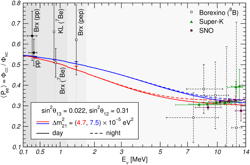
Figure 1: Dependence of the probabilities $P_{ee}$ integrated over the day and night time periods, for $\Delta m^{2}_{21}$ determined from the global fit of the solar neutrino data only (red) and from the global fit of all oscillation data (blue). Also shown are the results from different experiments. We use abbreviations “Brx” for Borexino and “KL” for KamLAND.

Fig. 1 shows dependence of the probabilities $P_{ee}(E)$ integrated over the day and the night times. At low energies neglecting the $\nu_{e}$ regeneration one has

$$P_{ee}\approx c_{13}^{4}(1-0.5\sin^{2}2\theta_{12})-0.5c_{13}^{6}\cos 2\theta_{12}\sin^{2}2\theta_{12}\epsilon_{12}\,.$$ (31)

With decrease of energy: $P_{ee}\to P_{ee}^{\text{vac}}$. For the best fit value of the 1-2 mass splitting deviations of the probability (31) from its vacuum values are $6\%$ for the ${}^{7}\text{Be}$-neutrinos and $2\%$ for the $pp$-neutrinos with $E=0.3~{}\text{MeV}$.

At high energies the matter effect dominates and

$$P_{ee}=c_{13}^{4}\sin^{2}\theta_{12}+c_{12}^{2}F_{\text{reg}}+\frac{1}{4}\cos 2\theta_{12}\sin^{2}2\theta_{12}\epsilon_{12}^{-2}\,.$$ (32)

The intermediate energy region between the vacuum and matter dominated limits is actually the region where the resonance turn on (turn off). The middle of this region (before averaging) corresponds to the MSW resonance at maximal densities in the Sun. Value of $\theta_{12}$ determines sharpness of the transition, that is, the size of transition region. The larger $\theta_{12}$ the bigger the size of the region. Integration over the neutrino production region in the Sun smears the transition, thus reducing the sensitivity to $\theta_{12}$.

As follows from Fig. 1 almost all experimental points are within $1\sigma$ from the prediction. Larger deviations can be seen in the intermediate region.

2.7 Scaling

The conversion probability of solar neutrinos obeys certain scaling which allows to understand various features of the LMA MSW solution as well as effects of new physics. The survival probability averaged over the oscillations on the way to the Earth (related to loss of propagation coherence) is function three dimensionless parameters:

$$P_{ee}=P_{ee}(\epsilon_{12},\epsilon_{13},\phi_{E})\,.$$ (33)

Here

$$\phi_{E}\approx\frac{\Delta m^{2}_{21}L}{2E}$$ (34)

is the phase of oscillations in the Earth and $\epsilon_{12}$, $\epsilon_{13}$ are defined in Eqs. (17), (19) correspondingly.

Several important properties follow immediately:

1. The probability is invariant with respect to rescaling

   $$\Delta m^{2}_{21}\to b\Delta m^{2}_{21}\,,\quad\Delta m^{2}_{31}\to b\Delta m^{2}_{31}\,,\quad E\to bE\,.$$ (35)

2. The adiabatic probability does not depend on distance and any spatial scale of the density profile. So, the only dependence on distance is in the phase $\phi_{E}$. If oscillations in the Earth are averaged, then whole the probability, $P_{ee}=P_{ee}(\epsilon_{12},\epsilon_{13})$, is scale invariant. This happens for practically all values of the zenith angle. In this case $P_{ee}$ is invariant with respect to rescaling

   $$\Delta m^{2}_{21}\to a\Delta m^{2}_{21}\,,\quad\Delta m^{2}_{31}\to a\Delta m^{2}_{31}\,,\quad V_{e}\to aV_{e}\,.$$ (36)

   In particular, if $a=-1$, $P_{ee}$ is invariant with respect to change of the signs of mass squared differences and potentials. Since the oscillation probability in the Earth (the regeneration factor) does not change under $\phi_{E}\to-\phi_{E}$, the invariance with respect to simultaneous change of signs of $\Delta m^{2}$ and potential (Eq. (36) with $a=-1$) holds also for the non-averaged probability (33).

3. If $|\Delta m^{2}_{31}|$ is kept fixed, the scaling (36) is broken by the 1-3 oscillations.

4. The dependence of the probability on $\epsilon_{13}$ is weak, and if neglected,

   $$P_{ee}\approx P_{ee}(\epsilon_{12})=P_{ee}\left(\frac{2V_{e}E}{\Delta m^{2}_{21}}\right)$$ (37)

   depends on one combination of the parameters only.

We will use these properties in the following discussion.

3 Determination of the neutrino parameters

The conversion effect of the solar neutrinos depends mainly on $\sin^{2}\theta_{12}$ and $\Delta m^{2}_{21}$. In the approximation $\sin^{2}\theta_{13}=0$ the problem is reduced to $2\nu$ problem. Due to low neutrino energies the 1-3 mixing, being small in vacuum, is not enhanced substantially in matter. Consequently, corrections to the $2\nu$ approximation are proportional to $\sin^{2}\theta_{13}$.

With increase of experimental accuracy dependence of the probability on the 1-3 mixing becomes visible. It is mainly via dependence of the elements of PMNS matrix $U_{e1}$ and $U_{e2}$ on $\cos^{2}\theta_{13}$.

Dependence of the probability on $\Delta m^{2}_{31}$ is via the matter correction to the 1-3 mixing (18). This correction is about $0.3\%$ at 10 MeV, that is, an order of magnitude smaller than correction due to the non-zero 1-3 mixing itself.

Similarly, the sensitivity of solar neutrinos to the 1-3 mass hierarchy (the sign of $\Delta m^{2}_{31}$) is low. According to Eq. (18) in the case of inverted mass hierarchy the correction to the $\sin^{2}\theta_{13}$ is negative. Consequently, the survival probability increases at high energies by about $0.5\%$ in comparison with the NH case.

Solar neutrinos are insensitive to the 2-3 mixing. The reason is that only the electron neutrinos are produced in the Sun, and $\nu_{\mu}$ and $\nu_{\tau}$ can not be distinguished at the detection.

Solar neutrino fluxes do not depend on the CP-violation phase $\delta$ Minakata:1999ze . Indeed, in the standard parametrization $|U_{ei}|$ do not contain $\delta$. In matter the propagation can be considered in the propagation basis, $\nu_{\text{prop}}$, defined as $\nu_{f}=U_{23}\Gamma_{\delta}\nu_{\text{prop}}$, where $U_{23}$ is the matrix of rotation in the ($\nu_{\mu}$, $\nu_{\tau}$) plane and $\Gamma_{\delta}\equiv\mathop{\mathrm{diag}}(1,1,e^{i\delta})$. In this basis the CP phase is eliminated from evolution, whereas $\nu_{e}$ is unchanged. As a result, the amplitude of probability, $A_{ee}$, does not depend on $\delta$.

3.1 The 1-2 mixing and mass splitting

The angle $\theta_{12}$ determines the energy dependence of the effect (24) (shape of the energy profile) via $\theta_{12}^{m}$ both in the Sun and the Earth. The oscillation phase is relevant only for oscillations in the Earth for a small range of zenith angles near horizon. Also in the first approximation the dependence of the probability on $\Delta m^{2}_{31}$ can be neglected. Then the whole the picture is determined by $\Delta m^{2}_{21}$ in combination with energy: $\Delta m^{2}_{21}/E$. This means that with change of $\Delta m^{2}_{21}$ the profile shifts in the energy scale by the same amount without change of its shape. In particular, with decrease of $\Delta m^{2}_{21}$ the same feature of the profile (e.g., the upturn) will show up at lower energies. Since dependence of the profile on $E$ is weak at large and small energies, it is the position of the transition region with respect to the solar neutrino spectrum that determines $\Delta m^{2}_{21}$.

Also the $\nu_{e}$ regeneration effect in the Earth depends on $\Delta m^{2}_{21}$: according to (26) $F_{\text{reg}}\propto 1/\Delta m^{2}_{21}$.

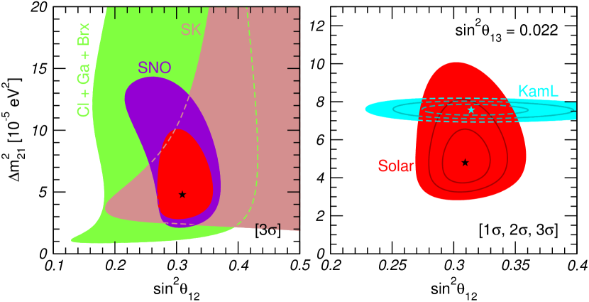
Figure 2: Allowed regions of $\theta_{12}$ and $\Delta m^{2}_{21}$ from the global fit of the solar neutrino data (red) as well as KamLAND (blue), for $\theta_{13}$ fixed to the best fit of the reactor experiments. In the lefts panel shown are also regions restricted by individual experiments.

In Fig. 2 we show result of the global fit of the solar neutrino data in the ($\theta_{12}$, $\Delta m^{2}_{21}$) plane, for $\theta_{13}$ fixed to the best fit value from the reactor experiments. In the left panel we show the regions restricted by individual solar neutrino experiments, whereas in the right panel we compare the solar and KamLAND allowed regions. The preferred value of $\theta_{12}$ from the analysis of solar data slightly increases as $\theta_{13}$ increases. Compared to the solar neutrino analysis KamLAND gives about $2\sigma$ larger $\Delta m^{2}_{21}$ but practically the same value of $\theta_{12}$.

3.2 The 1-2 mass ordering

Solar neutrinos allow to fix the sign of $\Delta m^{2}_{21}$ for the standard value of $V_{e}$. The sign determines the resonance channel (neutrino or antineutrino) and the mixing in matter. The facts that due to smallness of the 1-3 mixing the problem is reduced approximately to the $2\nu$-problem and that suppression of signal averaged over the oscillations at high energies is stronger than $1/2$, selects $\Delta m^{2}_{21}>0$. That corresponds to the normal ordering (hierarchy) when the electron flavor is mostly present in the lightest state.

For both signs of $\Delta m^{2}_{21}$ consideration and formulas are the same and the only difference is the value of $\theta_{12}^{m}(n_{e}^{0})$ in the production point. For high energies when density at production is much bigger than the resonance one $n_{e}^{0}\gg n^{res}(E)$, one has $\cos 2\theta_{12}^{m}\approx-1$ ($+1$) for normal (inverted) ordering. Correspondingly, the ratio of probabilities in the NH and IH cases equals $\tan^{2}\theta_{12}\approx 1/2$. Thus, for inverted ordering the suppression would weaken with increase of energy.

According to Eq. (30) with change of the sign of $\Delta m^{2}_{21}$ the Earth matter effect (regeneration factor) flip the sign.

3.3 The 1-3 mixing

If $s_{13}^{4}$ terms in the probability (13) are neglected, dependence on the 1-3 appears as an overall normalization which can be absorbed (at least partially) in uncertainties of neutrino fluxes. In contrast, degeneracy of the 1-2 and 1-3 mixings is absent since $\sin^{2}\theta_{12}$ and $\sin^{2}\theta_{13}$ enter the probability $P_{ee}$ in different combinations in the vacuum and matter dominated energy regions. According to (31) and (32) these combinations are

$$s_{13}^{2}\approx\frac{1}{2}-\frac{P^{h}}{2s_{12}^{2}}\,,\qquad s_{13}^{2}\approx\frac{1}{2}-\frac{P^{l}}{2-\sin^{2}2\theta_{12}}\,.$$ (38)

The SNO and SK results on the one hand side, and Borexino (${}^{7}\text{Be}$-, $pp$-neutrinos), and to a large extent Ga-Ge results on the other depend on different combinations of angles $\theta_{12}$ and $\theta_{13}$. Fig. 3 shows the allowed region in the plane $\sin^{2}\theta_{12}-\sin^{2}\theta_{13}$. The left panel illustrates how the low and high energy data restrict the allowed region. Also shown is the result of global fit of all solar neutrino data which gives smaller $\Delta m^{2}_{21}$ and the best fit value $\sin^{2}\theta_{13}=0.017$. The latter coincides with the earlier result in Ref. Goswami:2004cn .

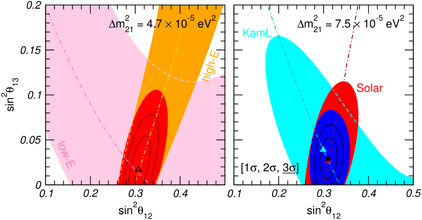
Figure 3: Allowed regions of mixing angles $\theta_{12}$ and $\theta_{13}$ from the global fit of the solar neutrino data only (left) and the solar plus KamLAND data (right).

Instead of low energy solar neutrino data one can use the KamLAND antineutrino result (vacuum oscillations with small matter corrections). Result of the combined fit of the solar and KamLAND data in assumption of the CPT invariance is shown in Fig. 3 (right). KamLAND data shift the 1-3 mixing to bigger value: $\sin^{2}\theta_{13}=0.028$. The present solar neutrino accuracy on $\theta_{13}$ is much worse than the one from the reactor experiments, but it can be substantially improved in future by SNO+, JUNO, Hyper-Kamiokande.

3.4 Tests of theory of neutrino oscillations and conversion

3.4.1 Determination of the matter potential

As discussed in the previous sections, the MSW effect plays central role in the solution of the solar neutrino problem. It is therefore important to experimentally verify all the aspects of this effect, and in particular, value of matter potential. To this end, we follow the approach of Ref. Fogli:2003vj and allow for an overall rescaling of the matter potential:

$$V_{e}\to a_{\textsc{msw}}V_{e}\,.$$ (39)

Note that such a modification of the matter term can be regarded as a special case of non-standard neutrino interactions Gonzalez-Garcia:2013usa , which we will describe in detail in Sec. 4.2.

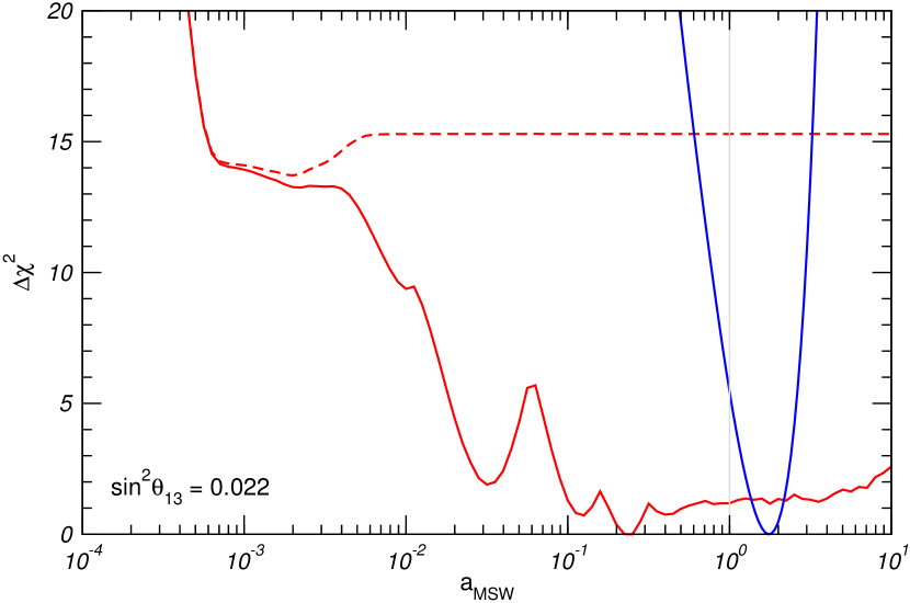
Figure 4: Determination of the matter potential from the solar (red) and solar+KamLAND (blue) neutrino data, as a function of the scaling parameter $a_{\textsc{msw}}$. We fix $\sin^{2}\theta_{13}=0.022$ and $\Delta m^{2}_{31}\to\infty$, and marginalize over $\Delta m^{2}_{21}$ and $\theta_{12}$. The dashed red line is obtained neglecting the Earth matter effect.

In order to determine the preferred value and allowed range of $a_{\textsc{msw}}$, we perform a fit of the solar neutrino data only (Fig. 4, red line) and a combined fit of the solar and KamLAND neutrino data (blue line). We fix for simplicity $\sin^{2}\theta_{13}=0.022$ but allow $\theta_{12}$ and $\Delta m^{2}_{21}$ to vary freely. We find $0.84\leq a_{\textsc{msw}}\leq 3.08$ at the $3\sigma$ level (see Fig. 4, blue line), with best-fit value $a_{\textsc{msw}}=1.66$. The standard value $a_{\textsc{msw}}=1$ is well within the allowed region, although slightly disfavored by the data ($\Delta\chi^{2}=5$). As we will see in Sec. 4.2, this is related to the tension between solar and KamLAND data in the determination of $\Delta m^{2}_{21}$, which can be alleviated by a non-standard matter potential.

Inclusion of the KamLAND data is essential for determination of $a_{\textsc{msw}}$. Indeed, as long as scaling (37) is realized ($P_{ee}$ depends only on the combination $V_{e}/\Delta m^{2}_{21}$), a rescaling of the matter potential $V_{e}$ can be compensated by the same rescaling of $\Delta m^{2}_{21}$. This is clearly reflected by the dashed red line in Fig. 4, for which the Earth matter effect has been “switched off”.

According to Fig. 4, scaling (37) is broken in the range $3\times 10^{-3}\lesssim a_{\textsc{msw}}\lesssim 0.3$ by the effect of non-averaged oscillations in the Earth, which for small $\Delta m^{2}_{21}$ depend on $L$. This is seen as wiggles of the red solid line. Violation of scaling at $a_{\textsc{msw}}\lesssim 5\times 10^{-3}$ corresponds to the breaking of adiabaticity in the Sun, so that formula for $P_{ee}$ becomes invalid. In this range $l_{\nu}>0.1R_{\text{sun}}$. The sharp increase of $\Delta\chi^{2}$ at $a_{\textsc{msw}}\sim 5\times 10^{-4}$ (very small $\Delta m^{2}_{21}$) occurs when $l_{\nu}\sim R_{\text{sun}}$.

Thus, the solar neutrinos alone give only the lower bound $a_{\textsc{msw}}>5\times 10^{-3}$, and can not fix $V_{e}$ and $\Delta m^{2}_{21}$. The precise matter-independent determination of $\Delta m^{2}_{21}$ provided by KamLAND fixes the issue.

According to Fig. 4 at $a_{\textsc{msw}}\sim 1$ the Earth matter effect reduces $\chi^{2}$ by $\Delta\chi^{2}\sim 14$, i.e., the effect is seen at about $4\sigma$, when all the data (in particular, SNO) are included.

3.4.2 Oscillation phase

Results of global analysis of the solar neutrino data can be compared with results from non-solar experiments which have different environment, type of neutrino, energy, etc. This comparison provides important possibility to test the theory of oscillations and to search for new physics.

As an example, suppose that for some geometrical reasons, non-locality, etc., the phase in the oscillation formula differs from the standard one by a factor $\xi$:

$$\phi\to\xi\phi$$ (40)

as it was advocated in some publications earlier. This means that $\Delta m^{2}_{21}$ extracted from the corresponding measurements would be different by a factor $1/\xi$. If the factor $\xi$ does not appear in the Hamiltonian, one can establish existence of $\xi\neq 1$ using $\Delta m^{2}_{21}$ from the adiabatic conversion result which does not depend on the phase. The fact that $\Delta m^{2}_{21}$ obtained from solar neutrino data and KamLAND are close to each other allows to restrict $\xi$.

Comparing results from KamLAND measurement and solar neutrino experiments one can search for effects of CPT violation, presence of non-standard interactions, etc.

3.5 Status of the LMA MSW. Open issues

LMA MSW gives good description of all existing solar neutrino data with their present accuracy and no statistically significant deviation are found. The LMA solution reproduces all the observed features including the directly measured $pp$-neutrino flux Bellini:2014uqa , as well as the Day-night asymmetry: $(2-4)\%$ for the boron neutrinos Renshaw:2013dzu and the value consistent with zero for ${}^{7}\text{Be}$-neutrinos Bellini:2011yj . Pulls of different measurements with respect to predictions for the best-fit values of oscillation parameters extracted from the solar neutrino data can be seen in Fig. 1. There is certain redundancy of measurements from different experiments which provides consistency checks of the results.

Realization of the KamLAND experiment Suzuki:2014woa was motivated by the solar neutrinos studies, namely by a possibility to test the LMA solution. Although historically by measuring $\Delta m^{2}_{21}$ KamLAND has uniquely selected the LMA solution, now the solar neutrino experiments alone can do this due to new measurements by Borexino, which validated the solution at low energies, and due to higher accuracy of other results.

There are a few open issues which motivate further detailed studies. Three following facts are most probably related:

1. The “upturn” of the spectrum (the ratio of the measured spectrum to the SSM one) towards low energies is not observed. According to the LMA solution the suppression should weaken with decrease of energy is not observed (see fig. 1). The increase should be for all energies (if oscillations in the Earth are not included) but the strongest change is expected in the range $(2-6)~{}\text{MeV}$. With oscillations in the Earth also the upturn towards high energies is expected. No one experiment has showed the upturn. The SNO experimental points even turn down at low energies.

2. For the best fit values from the global solar neutrino fit, one expects the D-N asymmetry $A_{\textsc{dn}}\equiv 2(N-D)/(N+D)=2.8\%$. For values of $\Delta m^{2}_{21}$ from global fit of all oscillation data (dominated by KamLAND) the asymmetry equals $A_{\textsc{dn}}=1.8\%$. Super-Kamiokande gives larger value: $A_{DN}=(3.2\pm 1.1\pm 0.5)\%$ Renshaw:2013dzu , and even larger asymmetry, $4.2\%$, has been obtained from separate day and night measurements. This can be simply statistical fluctuation. Especially in view of the observed energy and zenith angle dependencies of the asymmetry.

3. The 1-2 mass splitting extracted from the global fit of the solar neutrino data $\Delta m^{2}_{21}=(4.7^{+1.6}_{-1.1})\times 10^{-5}~{}\text{eV}^{2}$ is about $2\sigma$ smaller than the value measured by KamLAND (antineutrino channel) as well as the global fit value of all oscillation data Gonzalez-Garcia:2014bfa $\Delta m^{2}_{21}=(7.50_{-0.17}^{+0.19})\times 10^{-5}~{}\text{eV}^{2}$. Notice that the bump in the spectrum of reactor antineutrinos at $(4-6)~{}\text{MeV}$ uncovered recently Seo:2014jza ; Zhan:2015aha leads to a decrease of $\Delta m^{2}_{21}$ extracted from KamLAND data by about $0.1\times 10^{-5}~{}\text{eV}^{2}$, and therefore to an insignificant reduction of the disagreement Maltoni15 . With the decrease of $\Delta m^{2}_{21}$ the upturn and regeneration peak shift to lower energies, which leads to weaker distortion of the spectrum at low energies and larger D-N asymmetry.

4. The value of potential extracted from the solar neutrino data is larger by a factor 1.6 than the standard potential. This is directly related to difference of $\Delta m^{2}_{21}$ extracted from the solar and KamLAND data (Sec. 3.4).

Solar neutrino studies motivated calibration experiments with radiative sources. The latter led to Gallium anomaly – about $2\sigma$ deficit of signal which implies new physics unrelated to the solar neutrinos (and has value by itself). Impact of the Gallium calibration on results of solar neutrino experiments is not strong if it is related to cross-section uncertainties in the energy range of calibration sources.

3.6 Theoretical and phenomenological implications

Measured oscillation parameters have important implications for fundamental theory, though there is no unique interpretation. The observed 1-2 mixing is large but not maximal. The deviation of the measured value $\sin^{2}\theta_{12}=0.304^{+0.013}_{-0.012}$ is about $15\sigma$ below $\sin^{2}\theta_{12}=0.5$ and it is substantially larger than $\sin^{2}\theta_{C}=0.050$. The value of $\sin^{2}\theta_{12}$ is in between of $\sin^{2}(\pi/4-\theta_{C})=0.281$ and $\sin^{2}\theta_{12}=1/3$, where the first number corresponds to the Quark Lepton Complementarity (QLC) Minakata:2004xt and the second one to the Tri-bimaximal (TBM) mixing Harrison:2002er . In turn, QLC implies a kind of quark-lepton unification (symmetry), and probably, the Grand Unification (GU). TBM indicates toward geometric origins of mixing and certain flavor symmetry which is realized in the residual symmetries approach Lam:2008sh ; Lam:2008rs ; Grimus:2009pg .

Measured value of $\Delta m^{2}_{21}$ gives the lower bound on the mass $m_{2}\geq\sqrt{\Delta m^{2}_{21}}=0.007~{}\text{eV}$. Comparing $\Delta m^{2}_{21}$ with $\Delta m^{2}_{31}$ one finds that neutrinos have the weakest mass hierarchy (if any) among all other leptons and quarks in the case of normal mass ordering: $m_{2}/m_{3}\geq\sqrt{\Delta m^{2}_{21}/\Delta m^{2}_{31}}$ $=0.18$. In the case of inverted mass hierarchy $\Delta m^{2}_{21}$ determines degeneracy of two heavy mass states $\Delta m/m_{2}\geq\Delta m^{2}_{21}/2\Delta m^{2}_{31}=1.5\times 10^{-2}$, which implies certain flavor symmetry. If neutrinos are Majorana particles, their masses fix the effective scale of new physics responsible for the neutrino mass generation. For the $D=5$ Weinberg operator generating such a mass, we obtain the value new physics scale $\Lambda=v_{\text{EW}}^{2}/\sqrt{\Delta m^{2}_{21}}\sim 10^{16}~{}\text{GeV}$ which coincides essentially with the GU scale.

There is a number of phenomenological consequences of the solar neutrino results:

1. Supernova (SN) neutrinos: in outer regions of a collapsing star the MSW conversion produces significant flavor changes of fluxes. The conversion occurs in the adiabatic regime. Due to the 1-2 mass splitting and mixing the SN neutrinos oscillate in the matter of the Earth leading to the observable effects (see, e.g., Ref. Dighe:1999bi ).

2. The Early Universe: equilibration of the lepton asymmetries in different flavors occurs due to oscillations with large mixings Lunardini:2000fy ; Dolgov:2002ab .

3. Neutrinoless double beta decay: contribution from the second mass state to the effective Majorana mass of the electron neutrino gives the dominant contribution in the case of normal mass hierarchy: $m_{ee}^{(2)}\approx\sin^{2}\theta_{12}\sqrt{\Delta m^{2}_{21}}$ $=(2-3)~{}\text{meV}$. In the case of inverted hierarchy $m_{ee}\approx m_{ee}^{(1,2)}\propto c_{13}^{2}|\cos^{2}\theta_{12}+\sin^{2}\theta_{12}e^{i\phi}|$, and numerically $m_{ee}^{(1,2)}\approx(18-50)$ meV depending on value of the Majorana phase $\phi$.

4. CP-violation effects are proportional to $\sin 2\theta_{12}$, and $\Delta m^{2}_{21}$ determines the $L/E$ scale for oscillation experiments which are sensitive to the CP phase.

4 Solar neutrinos and physics beyond $3\nu$ framework

Apart from masses and mixing a number of non-standard neutrino properties have been considered which lead to new effects in propagation of neutrinos, and consequently, to suppression of the solar $\nu_{e}$ flux. After establishing LMA MSW solution, these effects can show up as subleading effects. Their searches in solar neutrinos allow to put bounds on standard neutrino properties.

As far as propagation is concerned, effects of new physics can be described by adding new terms, $H_{\textsc{np}}$, to the Hamiltonian in Eq. (1): $H\to H_{\textsc{lma}}+H_{\textsc{np}}$. In the following sections we will use the approximation of the third mass dominance, $\Delta m^{2}_{31}\to\infty$ or decoupling of $\nu_{3}$, according to which the evolution of 3 neutrinos (in certain basis) is reduced to the evolution of a $2\nu$ system described by an effective Hamiltonian $H^{(2)}=H_{\textsc{lma}}^{(2)}+H_{\textsc{np}}^{(2)}$ with

$$H_{\textsc{lma}}^{(2)}=\frac{\Delta m^{2}_{21}}{4E}\begin{pmatrix}-\cos 2\theta_{12}&\sin 2\theta_{12}\\ \hphantom{+}\sin 2\theta_{12}&\cos 2\theta_{12}\end{pmatrix}+\sqrt{2}G_{F}n_{e}\begin{pmatrix}c_{13}^{2}&0\\ 0&0\end{pmatrix}.$$ (41)

In addition, new physics can affect production and interactions of neutrinos, which we will discuss separately for each specific case.

4.1 Sterile neutrinos

Sterile neutrinos, singlets of the standard model symmetry group, can manifest themselves through mixing with ordinary neutrinos, with non-trivial implications for the oscillation patterns. The most general neutrino mass matrix which generates such a mixing with $n$ sterile neutrinos has in the basis $\nu_{f}=(\nu_{e},\nu_{\mu},\nu_{\tau},\nu_{s1},\dots,\nu_{sn})^{T}$ a form

$$\mathcal{M}_{\nu}=\begin{pmatrix}0&m_{D}\\ m_{D}^{T}&m_{N}\end{pmatrix},$$ (42)

where $m_{D}$ is a generic $3\times n$ matrix and $m_{N}$ is a $n\times n$ symmetric matrix. Then the Hamiltonian in vacuum equals $H_{0}=\mathcal{M}_{\nu}\mathcal{M}_{\nu}^{\dagger}/2E$. The diagonal matrix of the matter potentials appearing in (1) is now $V=\mathop{\mathrm{diag}}(V_{e}+V_{n},V_{n},V_{n},0,\dots,0)$ with $V_{n}=-(1/\sqrt{2})G_{F}n_{n}$ and $n_{n}$ being the number density of neutrons.

From a phenomenological point of view, three different regimes can be identified, depending on whether the mass-squared splitting involving the sterile neutrinos, $\Delta m^{2}_{\text{as}}$, is much smaller, comparable, or much larger than $\Delta m^{2}_{21}$.

4.1.1 $\Delta m^{2}_{\text{as}}\ll\Delta m^{2}_{21}$: quasi-Dirac case

This was realized in the “Just-so” solution of the solar neutrino problem. For very small Majorana masses, $|m_{N}|\ll|m_{D}|$, the eigenvalues of Eq. (42) form pairs of almost degenerate states. This situation is referred as “quasi-Dirac” limit. The presence of extra mass-squared splittings can distort the neutrino oscillation patterns, and due to very big baseline (the Sun-Earth distance) the solar neutrino experiments have high sensitivity to small values of $|m_{N}|$. For $\Delta m^{2}_{\text{as}}<10^{-9}~{}\text{eV}^{2}$ the evolution inside the Sun is practically unaffected by the presence of the sterile neutrinos (the oscillations into sterile neutrinos are suppressed in matter), and the main effect is due to vacuum oscillations $\nu_{a}\to\nu_{s}$ on the way from the Sun to the Earth.

In order not to spoil the accurate description of solar oscillations data the Majorana mass should satisfy the upper bound $|m_{N}|\lesssim 10^{-9}~{}\text{eV}$ (normal ordering) or $|m_{N}|\lesssim 10^{-10}~{}\text{eV}$ (inverted ordering) deGouvea:2009fp ; Donini:2011jh . The bound corresponds to the maximal active sterile mixing and $\Delta m^{2}_{\text{as}}\approx 2m_{D}m_{N}=(10^{-11}-10^{-9})~{}\text{eV}^{2}$.

4.1.2 $\Delta m^{2}_{\text{as}}\lesssim\Delta m^{2}_{21}$

Originally, this possibility has been motivated by relatively low $Ar$- production rate in the Homestake experiment and absense of spectral upturn deHolanda:2003tx ; deHolanda:2010am . An extra sterile state has been added to the three active ones, $\nu_{f}=(\nu_{s},\nu_{e},\nu_{\mu},\nu_{\tau})^{T}$, and correspondingly, new mass state $\nu_{0}$: $\nu_{m}=(\nu_{0},\nu_{1},\nu_{2},\nu_{3})^{T}$. The $4\times 4$ mixing matrix is parametrized as $U=U_{\text{PMNS}}\,U_{01}(\alpha)$ deHolanda:2003tx . The value of new mixing angle is assumed to be very small: $\sin^{2}2\alpha\sim 10^{-3}$ and the new mass splitting equals $\Delta m^{2}_{01}\sim 0.2\Delta m^{2}_{21}~{}\text{eV}^{2}$. The diagonal matrix of the matter potentials in the flavor basis is $V=\mathop{\mathrm{diag}}(0,V_{e}+V_{n},V_{n},V_{n})$.

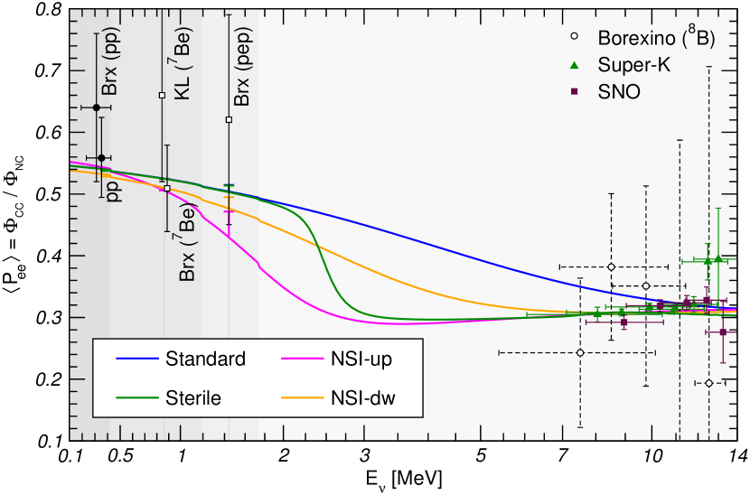
Figure 5: Impact of new physics on solar neutrino survival probability. We fix $\sin^{2}\theta_{13}=0.022$. We plot standard oscillations ($\sin^{2}\theta_{12}=0.31$, $\Delta m^{2}_{21}=7.5\times 10^{-5}~{}\text{eV}^{2}$), one extra sterile neutrino ($\sin^{2}\theta_{12}=0.31$, $\Delta m^{2}_{21}=7.5\times 10^{-5}~{}\text{eV}^{2}$, $\sin^{2}2\alpha=0.005$, $\Delta m^{2}_{01}=1.2\times 10^{-5}~{}\text{eV}^{2}$) and non-standard interactions with up-type ($\sin^{2}\theta_{12}=0.30$, $\Delta m^{2}_{21}=7.25\times 10^{-5}~{}\text{eV}^{2}$, $\varepsilon_{D}^{u}=-0.22$, $\varepsilon_{N}^{u}=-0.30$) and down-type ($\sin^{2}\theta_{12}=0.32$, $\Delta m^{2}_{21}=7.35\times 10^{-5}~{}\text{eV}^{2}$, $\varepsilon_{D}^{d}=-0.12$, $\varepsilon_{N}^{d}=-0.16$) quarks. See text for details. We use abbreviations “Brx” for Borexino and “KL” for KamLAND.

In such a model, the neutrinos propagating inside the Sun encounter two resonances: one is associated with the 1-2 mass splitting, as in the standard case, and another one with the 0-1 mass splitting. With parameters $\alpha$ and $\Delta m^{2}_{01}$ defined above the new resonance modifies the survival probability leading to the dip at the intermediate energies, $E\sim 3~{}\text{MeV}$, thus suppressing the upturn (see Fig. 5). This alleviates the tension between solar and KamLAND data.

4.1.3 $\Delta m^{2}_{\text{as}}\gg\Delta m^{2}_{21}$

In this limit (see Refs. Palazzo:2011rj ; Kopp:2013vaa for latest discussions) all the $\Delta m^{2}_{ij}$ other than $\Delta m^{2}_{21}$ can be assumed to be infinite, and in certain propagation basis the neutrino evolution is described by the sum of $H_{\textsc{lma}}^{(2)}$ in Eq. (41) and

$$H_{\textsc{np}}^{(2)}=\sqrt{2}G_{F}\frac{n_{n}}{4}\begin{pmatrix}-\xi_{D}&~{}\xi_{N}e^{-i\delta_{12}}\\ \hphantom{-}\xi_{N}e^{i\delta_{12}}&~{}\xi_{D}\end{pmatrix},$$ (43)

where $\xi_{D}$, $\xi_{N}$ are combinations of the mixing matrix elements $U_{\alpha i}$ (explicit expressions can be found in App. C of Ref. Kopp:2013vaa ).

The new physics term (43) proportional to $V_{n}$, is induced by the decoupling of heavy neutrino states. In general, the matter term (43) and the usual one with $V_{e}$ do not commute with each other as well as with the vacuum term. The phase $\delta_{12}$ appearing in $H_{\textsc{np}}^{(2)}$ originates from the phases of the general $(3+n)$ mixing matrix, and it cannot be eliminated by a redefinition of the fields. This phase does not produce CP-violation asymmetry but affects neutrino propagation in matter.

The relevant conversion probabilities can be written as

$$P_{ee} =\tilde{C}_{e}-\eta_{e}^{2}P_{\text{osc}}^{(2)}\,,$$ (44)

$$P_{ae} =\tilde{C}_{a}-\eta_{e}\left(\xi_{D}P_{\text{osc}}^{(2)}+\xi_{N}P_{\text{int}}^{(2)}\right),$$

where $P_{\text{osc}}^{(2)}\equiv|S_{21}^{(2)}|^{2}$ and $P_{\text{int}}^{(2)}\equiv\mathop{\mathrm{Re}}\big{(}S_{11}^{(2)}S_{21}^{(2)\star}\big{)}$ and the matrix $S^{(2)}$ is the solution of the evolution equation with the effective Hamiltonian $H^{(2)}$. The coefficients $\tilde{C}_{e}$, $\tilde{C}_{a}$, and $\eta_{e}$ are functions of $U_{\alpha i}$ Kopp:2013vaa . The formulas (44) are valid for any number of sterile neutrinos. Sterile neutrinos affect the oscillation probabilities in two different ways:

1. the mixing of $\nu_{e}$ with the “heavy” states leads to a suppression of the energy-dependent part of the conversion probabilities, in analogy with $\theta_{13}$ effects in the standard case;

2. the mixing of the sterile states with $\nu_{1,2}$ leads to overall disappearance of active neutrinos, so that $P_{ee}+P_{\mu e}+P_{\tau e}\neq 1$.

Phenomenologically, the most relevant effect is the second one, since the precise NC measurement performed by SNO confirms that the total flux of active neutrinos from the Sun is compatible with the expectations of the Standard Solar Model. Hence the fraction of sterile neutrinos which can be produced in solar neutrino oscillations is limited by the precision of the solar flux predictions, in particular of the Boron flux. An updated fit of the solar and KamLAND data in the context of (3+1) oscillations, with the simplifying assumption $U_{e3}=U_{e4}=0$, yields $|U_{s1}|^{2}+|U_{s2}|^{2}<0.1$ at the 95% CL.

Concerning the first effect, the mixing of $\nu_{e}$ with “heavy” eigenstates has similar implications as in the standard case except that now there are “more” heavy states. This allows to put a bound on $\eta_{e}$ which is very similar to the one on $|U_{e3}|^{2}$ in $3\nu$ one, but instead of being interpreted as a bound on $|U_{e3}|^{2}$ it becomes a bound on the sum $\sum_{i\geq 3}|U_{ei}|^{2}$. For example, for (3+1) models a bound $|U_{e3}|^{2}+|U_{e4}|^{2}<0.077$ at 95% CL can be derived from the analysis of solar and KamLAND data, as shown in Ref. Kopp:2013vaa . Additional bounds have been obtained by Borexino Bellini:2013uui .

4.2 Non-standard interactions

In the presence of physics Beyond the Standard Model, new interactions may arise between neutrinos and matter. They can lead to effective four-fermion operators of the form

$$\mathcal{L}_{\text{NSI}}=-2\sqrt{2}G_{F}\varepsilon_{\alpha\beta}^{fP}(\bar{\nu}_{\alpha}\gamma^{\mu}\nu_{\beta})(\bar{f}\gamma_{\mu}Pf)\,,$$ (45)

where $f$ denotes a charged fermion, $P\in\{L,R\}$ are the left and right projection operators and $\varepsilon_{\alpha\beta}^{fP}$ parametrize the strength of the non-standard interactions.

The non-standard interactions (NSI) were introduced to obtain oscillations w1a ; w1b or MSW conversion Roulet:1991sm ; Guzzo:1991hi without neutrino masses. NSI could provide an alternative solution of the solar neutrino problem. They can modify the LMA MSW solution, and inversely, be restricted by solar neutrinos Friedland:2004pp ; Palazzo:2009rb ; Bolanos:2008km ; Miranda:2004nb ; Guzzo:2004ue .

NSI affect neutrino propagation: the matter term, $V$, in the evolution equation (1) includes an extra contribution from NSI

$$V_{\alpha\beta}=V_{e}\delta_{\alpha e}\delta_{\beta e}+\sqrt{2}G_{F}\sum_{f}n_{f}\,\varepsilon_{\alpha\beta}^{f},$$ (46)

where $\varepsilon_{\alpha\beta}^{f}=\varepsilon_{\alpha\beta}^{fL}+\varepsilon_{\alpha\beta}^{fR}$. Hermiticity requires that $\varepsilon_{\beta\alpha}^{f}=\varepsilon_{\alpha\beta}^{f*}$, so that the diagonal entries $\varepsilon_{\alpha\alpha}^{f}$ must be real. The new physics part of the Hamiltonian equals

$$H_{\textsc{np}}^{(2)}=\sqrt{2}G_{F}\sum_{f}n_{f}\begin{pmatrix}-\varepsilon_{D}^{f\hphantom{*}}&\varepsilon_{N}^{f}\\ \hphantom{+}\varepsilon_{N}^{f*}&\varepsilon_{D}^{f}\end{pmatrix},$$ (47)

where $\varepsilon_{D}^{f}$ and $\varepsilon_{N}^{f}$ are linear combinations of the original parameters, $\varepsilon_{\alpha\beta}^{f}$, and their explicit expressions can be found in Ref. Gonzalez-Garcia:2013usa .

Neglecting matter effect on the 1-3 mixing one obtains that the $\nu_{e}$ probability $P_{ee}$  can be written as $P_{ee}=c_{13}^{4}P_{\text{surv}}^{(2)}+s_{13}^{4}$, where $P_{\text{surv}}^{(2)}\equiv|S_{11}^{(2)}|^{2}$ should be calculated using the Hamiltonian $H^{(2)}$.

In the specific case of NSI with electrons ($f=e$) both the standard and the non-standard (Eq. (47)) terms scale with the same matter density profile $n_{e}$. This implies that large enough positive value of $\varepsilon_{D}^{e}$ can “flip the sign” of the matter term, so that the resonance will be realized for the inverted 1-2 hierarchy, $\Delta m^{2}_{21}<0$, in contrast to the usual case. There is therefore an unresolvable degeneracy between the sign of $\Delta m^{2}_{21}$ and that of the matter potential: only their relative sign can be determined by oscillation experiments. For NSI with up-quarks ($f=u$) or down-quarks ($f=d$) this ambiguity is only approximate, however present data are unable to resolve it. As a consequence, in the presence of NSI the sign of $\Delta m^{2}_{21}$ can no longer be determined uniquely.

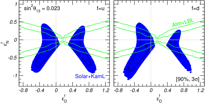
Figure 6: Allowed regions of parameters of the non-standard neutrino interaction (see text).

With new interactions the evolution inside the Sun is still adiabatic, and so the results are determined by the mixing at the production point. The latter is affected by NSI, and now also the off-diagonal elements of the Hamiltonian depend on matter potential. This means that at large values of the potential mixing is not suppressed: in asymptotics, $E\to\infty$, one has

$$\cos 2\theta_{m}\approx-\frac{c_{13}^{2}-2r_{f}\varepsilon_{D}^{f}}{\sqrt{(2r_{f}\varepsilon_{D}^{f}-c_{13}^{2})^{2}+(2r_{f}\varepsilon_{N}^{f})^{2}}},$$ (48)

where $r_{f}\equiv n_{f}/n_{e}$. According to Eq. (48), $\cos 2\theta_{m}>-1$, and therefore suppression at high energies for the same vacuum mixing is always weaker than without NSI. The mixing at the exit from the Sun coincides with the vacuum mixing. In the limit of very low energies $P_{ee}$ approaches the vacuum value as in the standard case. The strongest modification appears in the intermediate energy region. In general, the probability is given by (13) with

$$\cos 2\theta_{m}\approx-\frac{A}{\sqrt{A^{2}+(2r_{f}\varepsilon_{N}^{f}+\sin 2\theta_{12}\epsilon_{12}^{-1})^{2}}},$$ (49)

where $A\equiv-\cos 2\theta_{12}\epsilon_{12}^{-1}+c_{13}^{2}-2r_{f}\varepsilon_{D}^{f}$. The absolute minimum is achieved when the second term in denominator of (49) is zero, i.e.

$$\varepsilon_{N}^{f}=-\frac{\sin 2\theta_{12}}{2r_{f}\epsilon_{12}}.$$ (50)

This corresponds to zero the off-diagonal elements of Hamiltonian (47). For $E=3~{}\text{MeV}$ we obtain $\varepsilon_{N}^{f}=-0.3$.

In Fig. 5 we plot the $P_{ee}$ survival probability for non-standard interactions with up-quarks and down-quarks. As can be seen, the presence of NSI allows to considerably flatten the spectrum above $3~{}\text{MeV}$, in analogy with the similar effect produced by light sterile neutrinos. Moreover, NSI can also generate large day-night asymmetries: $(4-5)\%$ at $10~{}\text{MeV}$ for both cases, $f=u$ and $f=d$. The flattening and larger asymmetry remove the tension with KamLAND data.

The NSI and sterile neutrino cases can be distinguished by the slower increase of the NSI probability as the energy decreases. The sharp increase for the sterile case is related to small $\nu_{e}-\nu_{s}$ mixing (narrow resonance). The two possibilities can be distinguished, e.g., by precise measurements of the $pep$ neutrino flux and well as the day-night asymmetry at high energies.

The NSI provide a very good fit to solar neutrino data, even in the limit of $\Delta m^{2}_{21}=0$. This is mainly due to the lack of experimental data below $5~{}\text{MeV}$, where the transition between the MSW and the vacuum-dominated regime takes place. It is therefore not possible to obtain a precise determination of both vacuum oscillation and non-standard interaction parameters using only solar data. On the other hand, KamLAND measurement of $\Delta m^{2}_{21}$, being only marginally affected by matter effects, is rather stable under the presence of NSI. A combined fit of both solar and KamLAND data is therefore able to constraint both sets of parameters with good accuracy. In Fig. 6 we show the results of such a combined fit for NSI with $f=u$ (left) and $f=d$ (right), limited for simplicity to the case of real $\varepsilon_{N}^{f}$. The presence in both cases of two disconnected regions is related to the ambiguity in the determination of the sign of $\Delta m^{2}_{21}$ discussed above. Namely, the left-side regions include the standard solution $\varepsilon_{D}^{f}=\varepsilon_{N}^{f}=0$ $\Delta m^{2}_{21}>0$, the right-side regions (slightly disfavored for $f=d$) correspond to $\Delta m^{2}_{21}<0$.

In Fig. 6 the best fit points (stars) for solar+KamLAND are $\varepsilon_{D}^{d}=-0.12$ and $\varepsilon_{N}^{d}=-0.16$ for NSI with down-type quarks, and $\varepsilon_{D}^{u}=-0.22$ and $\varepsilon_{N}^{u}=-0.30$ for NSI with up-type quarks. These values are somewhat in tension with the atmospheric and LBL experiments bounds, and probably hard to accommodate within BSM models, although some possibility has been discussed Farzan:2015doa . As shown in Ref. Gonzalez-Garcia:2013usa , atmospheric and long-baseline data are insensitive to $\varepsilon_{D}^{f}$ but more restrictive for $\varepsilon_{N}^{f}$, and can therefore provide complementary information.

In addition to propagation effects, the presence of NSI can also affect the neutrino cross-sections relevant for neutrino detection. For example, in Ref. Agarwalla:2012wf stringent bounds on NSI with electrons were derived from the Borexino data by studying the elastic scattering in the ${}^{7}\text{Be}$ energy window.

4.3 Large magnetic moments

Electromagnetic interactions of neutrinos are due to neutrino dipole moments (see review Giunti:2014ixa ). The Dirac neutrino in the Standard Model has a very tiny magnetic moment, $\mu_{\nu}=3\times 10^{-19}\,(m_{\nu}/\text{eV})\,\mu_{B}$ Ref. Fujikawa:1980yx . Experimental evidence for a larger value of $\mu_{\nu}$ would therefore testify for the presence of some new physics physics.

Following the formalism of Ref. Grimus:2000tq , we describe the interaction of Dirac or Majorana neutrinos with the electromagnetic field in terms of an effective Hamiltonian in the flavor basis:

$$\mathcal{H}_{\text{em}}=\begin{cases}\hphantom{-}\dfrac{1}{2}\bar{\nu}_{R}\lambda\sigma^{\alpha\beta}\nu_{L}F_{\alpha\beta}+\text{h.c.}&\text{(Dirac),}\\[8.53581pt] -\dfrac{1}{4}\bar{\nu}_{L}^{T}C^{-1}\lambda\sigma^{\alpha\beta}\nu_{L}F_{\alpha\beta}+\text{h.c.}&\text{(Major.),}\end{cases}$$ (51)

where $C$ is the charge-conjugation operator and $\nu_{L(R)}^{T}=(\nu_{e},\nu_{\mu},\nu_{\tau})_{L(R)}$ is the vector of left-handed (right-handed) flavor states. The matrix $\lambda$ can be decomposed into the sum of two Hermitian matrices:

$$\lambda=\mu-id\,,\quad\mu=(\lambda+\lambda^{\dagger})/2\,,\quad d=i(\lambda-\lambda^{\dagger})/2\,.$$ (52)

Here $\mu$ describes the neutrino magnetic moments, while $d$ the electric dipole moments. The off-diagonal elements of these matrices link together states of opposite helicity and different flavors, and thus correspond to the transition moments Schechter:1981hw . For the Majorana neutrinos the CPT conservation implies that $\mu$ and $d$ are anti-symmetric imaginary matrices, so that their diagonal elements vanish and only transition moments are possible.

Bounds on the elements of the matrix $\lambda$ can be presented in terms of the collective quantity $|\Lambda|=\sqrt{\mathop{\mathrm{Tr}}(\lambda^{\dagger}\lambda)/2}$. For what concerns solar neutrinos, two effects of neutrino electromagnetic properties have been considered: neutrino spin-flavor precession and additional contribution to the neutrino-electron scattering cross-section.

4.3.1 Spin-flavor precession

The evolution of neutrino states under the combined influence of matter effects and strong magnetic fields, can be described by equation Lim:1987tk ; Akhmedov:1988uk ; Minakata:1988gm ; Grimus:2000tq :

$$i\frac{d}{dz}\begin{pmatrix}\varphi_{-}\\[5.69054pt] \varphi_{+}\end{pmatrix}=\begin{pmatrix}\dfrac{M^{\dagger}M}{2E}+V_{L}&-B_{+}\lambda^{\dagger}\\ -B_{-}\lambda&\dfrac{MM^{\dagger}}{2E}+V_{R}\end{pmatrix}\begin{pmatrix}\varphi_{-}\\[5.69054pt] \varphi_{+}\end{pmatrix},$$ (53)

where $\varphi_{+}$ and $\varphi_{-}$ denote the vectors of neutrino flavor states corresponding to positive and negative helicities, respectively. We have assumed that neutrino propagate along the $z$ direction, so that $B_{\pm}=B_{x}\pm iB_{y}$ are the components of the magnetic field perpendicular to the neutrino trajectory. Here $V_{L}=\mathop{\mathrm{diag}}(V_{e}+V_{n},V_{n},V_{n})$ is the standard matter potential for neutrino states; for Dirac neutrinos we have $V_{R}=0$, while for Majorana neutrinos we have $V_{R}=-V_{L}$.

The joint evolution of flavor and spin states induced by the existence of magnetic transition moments leads to the phenomenon of spin-flavor precession Lim:1987tk ; Akhmedov:1988uk ; Minakata:1988gm . The interplay of such mechanism and standard matter effects could be the source of the observed deficit of solar neutrinos, as long as $10^{-9}~{}\text{eV}^{2}\lesssim\Delta m^{2}_{21}\lesssim 10^{-7}~{}\text{eV}^{2}$ Miranda:2001hv ; Akhmedov:2002mf . However, the evidence for much larger $\Delta m^{2}_{21}$ provided by KamLAND, which is practically insensitive to small neutrino magnetic moment, ruled out this mechanism. Conversely, we can now use the precise determination of the oscillation parameters to set bounds on neutrino electromagnetic properties, by requiring that the accurate description of solar neutrino data is not spoiled by spin-flavor precession effects, and by the fact that no antineutrino coming from the sun is detected. For example, in Ref. Miranda:2004nz the bound $|\Lambda|\lesssim\text{few}\times 10^{-12}\,\mu_{B}$ for $\theta_{13}=0$ was derived, under the assumption that neutrinos are Majorana particles and that turbulent random magnetic fields exists in the Sun.

As can be seen in Eq. (53), in the presence of non-vanishing magnetic moment the evolution of the neutrino system mixes together positive and negative helicities, so that a conversion between them becomes possible. If neutrinos are Majorana particles this implies that neutrinos can convert into anti-neutrinos, which may result in the observation of a flux of anti-neutrinos coming from the Sun. Searches for $\bar{\nu}_{e}$ signal have been performed by both Borexino Bellini:2010gn and KamLAND Eguchi:2003gg , so far with negative results.

As shown in Ref. Miranda:2001hv , the large value of $\Delta m^{2}_{21}$, as measured by KamLAND, implies that a neutrino magnetic moment below $10^{-11}~{}\text{eV}^{2}$ has practically no effect on the evolution of solar neutrinos, given a characteristic solar magnetic field of the order of 80 kG.

4.3.2 Neutrino-electron cross-section

In the presence of magnetic moments extra term arises in the elastic neutrino-electron cross-section due to photon exchange:

$$\frac{d\sigma_{\text{em}}}{dT}=\frac{\alpha^{2}\pi}{m_{e}^{2}\mu_{B}^{2}}\left(\frac{1}{T}-\frac{1}{E}\right)\Big{(}\lVert\lambda\varphi_{-}^{\text{det}}\rVert^{2}+\lVert\lambda^{\dagger}\varphi_{+}^{\text{det}}\rVert^{2}\Big{)},$$ (54)

where $E$ is the neutrino energy, $T$ is the kinetic energy of the recoil electron, and the 3-vectors $\varphi_{-}^{\text{det}}$ and $\varphi_{+}^{\text{det}}$ denote the neutrino flavor amplitudes at the detector for negative and positive helicities.

In the case small precession effects in the Sun, the helicity of solar neutrinos is conserved, so that $\varphi_{+}^{\text{det}}=0$ and $\varphi_{-}^{\text{det}}$ can be calculated using the formalism introduced in Sec. 2. Following this formalism, in Ref. Grimus:2002vb a bound on Majorana transition moments was derived, $|\Lambda|\lesssim 6.3\times 10^{-10}\,\mu_{B}$ from the analysis of solar neutrino data alone, and $|\Lambda|\lesssim 2.0\times 10^{-10}\,\mu_{B}$ in combination with reactor antineutrino data. Such a bound can be improved by almost an order of magnitude after the inclusion of 3 years of Borexino data.

4.4 Neutrino decay

The existence of neutrino masses and flavour mixing implies that the heavier neutrino states decay into lighter ones, and are therefore unstable Bahcall:1972my . In the Standard Model, the neutrino lifetimes are much longer than the age of the Universe, hence well beyond the reach of present experiments. Observation of neutrino decay would therefore be a signal of New Physics.

In vacuum, the survival probability of an unstable state $\nu_{i}$ is described by an exponential factor $e^{-d_{i}L/E}$, where $E$ is the neutrino energy, $L$ is the traveled distance, and $d_{i}=m_{i}/\tau_{i}$ is the ratio of the neutrino mass and lifetime. Applying this to solar neutrinos and neglecting decay inside the Sun or across the Earth, we obtain

$$P_{e\alpha}=\sum_{i}P_{ei}^{S}P_{i\alpha}^{E}e^{-d_{i}L_{SE}/E},$$ (55)

where $P_{ei}^{S}$ and $P_{i\alpha}^{E}$ are the $\nu_{e}\to\nu_{i}$ and $\nu_{i}\to\nu_{\alpha}$ probabilities in the Sun and the Earth, respectively (see Sec. 2.2 and 2.4). If the decay daughter particles include lighter active neutrinos, they should be accounted for in the calculation of the event rates. Here we follow the approach of Refs. Berryman:2014qha ; Picoreti:2015ika and we ignore this possibility, thus assuming that decaying neutrinos simply “disappear”.

Due to the smallness of $\theta_{13}$ the impact of a nonzero $d_{3}$ on solar neutrino data is very small Berryman:2014qha . Indeed, from a global fit of the solar neutrino data we find that for $\sin^{2}\theta_{13}=0.022$ the values $d_{3}\gg 10^{-10}~{}\text{eV}^{2}$ (complete $\nu_{3}$ decay) are disfavored with respect to $d_{3}\ll 10^{-13}~{}\text{eV}^{2}$ (stable $\nu_{3}$ state) by $\Delta\chi^{2}=0.55$ only. Hence, no bound can be set on $d_{3}$ from the present data. On the other hand, from the same analysis we find $d_{1}=m_{1}/\tau_{1}<1.3\times 10^{-13}~{}\text{eV}^{2}$ and $d_{2}=m_{2}/\tau_{2}<1.2\times 10^{-12}~{}\text{eV}^{2}$ at the $3\sigma$ level, in a good agreement with the results of Refs. Berryman:2014qha ; Picoreti:2015ika . The global best fit point occurs for $d_{i}=0$, and the determination of the $\theta_{12}$ range is practically unaffected by the enlargement of the parameter space.

4.5 Violation of fundamental symmetries

Violation of fundamental symmetries (VFS) at the Planck mass scale is expected in theories attempting to unify gravity with quantum physics. Neutrinos, whose masses are generated by some physics close to the GUT/Planck scales, could be most sensitive to this violation. New effects in neutrino propagation may arise due to violations of the equivalence principle Gasperini:1988zf , neutrino couplings to space-time torsion fields DeSabbata:1981ek , violation of Lorentz invariance Coleman:1997xq and of CPT symmetry Colladay:1996iz . The impact of VFS on neutrino propagation can be accounted by the inclusion of extra terms in the Hamiltonian:

$$H_{\textsc{np}}^{(2)}=\frac{1}{2}\sigma^{\pm}E^{n}\begin{pmatrix}-\varphi_{D}&~{}\varphi_{N}\\ \hphantom{+}\varphi_{N}^{*}&~{}\varphi_{D}\end{pmatrix},$$ (56)

where $n$ is the energy power scaling, $\varphi_{D}$ and $\varphi_{N}$ parametrize the strength of the VFS effects, and $\sigma^{\pm}$ accounts for a possible relative sign between neutrinos and antineutrinos. We have ($n=1$, $\sigma^{+}=\sigma^{-}$) in the case of violation of the equivalence principle or violation of Lorentz invariance, ($n=0$, $\sigma^{+}=\sigma^{-}$) for neutrino couplings to space-time torsion fields, and ($n=0$, $\sigma^{+}=-\sigma^{-}$) for violation of CPT symmetry. $H_{\textsc{np}}$ does not involve matter or magnetic fields and therefore relevant also for propagation in vacuum.

The oscillation probabilities in the presence of VFS can be derived from the standard ones by just replacing the vacuum mixing and mass-squared splittings with effective quantities defined by diagonalizing the vacuum Hamiltonian. VFS can manifest itself through (A) deviation energy dependence of the oscillation length from $E^{-1}$, and (B) non-trivial dependence of the vacuum mixing parameters on the neutrino energy. So spectral information is necessary for searches of VFS.

Concerning solar neutrinos, a bound on the overall strength of VFS, $||\varphi||=\sqrt{|\varphi_{D}|^{2}+|\varphi_{N}|^{2}}$, can be estimated by requiring that the VFS term of Eq. (56) is not larger than the standard one, $||\varphi||E^{n}\lesssim\Delta m^{2}_{21}/E$. Using $\Delta m^{2}_{21}=\mathcal{O}(10^{-5}~{}\text{eV}^{2})$ and assuming a typical energy $E\approx 10~{}\text{MeV}$ (the scale at which spectral information is available from SK and SNO) we obtain $||\varphi||\lesssim 10^{-12}~{}\text{eV}$ for $n=0$ and $||\varphi||\lesssim 10^{-19}$ for $n=1$. Such estimations are consistent with results of numerical calculations.

4.6 Other new physics models

Practically any extension of the Standard Model, which leads to non-standard neutrino properties, produces observable effects in the neutrino oscillation pattern. The number of extensions which could be probed by solar neutrinos is therefore huge, and here we briefly mention few cases.

1. Mass Varying neutrinos were proposed in Ref. Fardon:2003eh to provide a theoretical framework for the otherwise unexplained closeness of values of the dark energy and dark matter densities today, even though their ratio varies in time as the third power of the cosmic scale factor. The model proposes that the dark energy and neutrino densities track each other, and that the neutrino mass is not a constant but rather a dynamical quantity arising from the minimization of an effective potential depending solely on the neutrino density itself.

   The phenomenological implications of this model for solar neutrinos were discussed in Ref. Cirelli:2005sg , where it was shown that the quality of the data fit is worse than in the standard case. A modification of the original model in which neutrino masses depend also on the density of visible matter was proposed in Kaplan:2004dq , and it was shown in Barger:2005mn that such a model is compatible with solar neutrino data.

2. The possible existence of other long-range forces beyond the electromagnetic and gravitational ones was first considered in Ref. Lee:1955vk . The phenomenological implications for solar neutrinos of a new leptonic force of this kind was discussed in Ref. GonzalezGarcia:2006vp . It was shown that such scenarios did not provide significant improvement of quality of the fit with respect to the standard LMA solution, and bounds on the strength and range of the new force were derived.

3. Non-standard decoherence effects are usually expected to be a possible manifestation of quantum gravity, for example in the presence of a “foamy” space-time fabric. The phenomenological implications of this mechanism for oscillating systems were first discussed in Ref. Ellis:1983jz . A concrete analysis applied to solar neutrinos was presented in Fogli:2007tx , where it was shown that the existence of non-standard sources of decoherence would induce extra smearing in the neutrino oscillation pattern and could therefore be detected experimentally. A fit to the available data showed no hint for such an effect, and stringent bounds on the new physics parameters were therefore derived.

4. The impact of extra dimensions on neutrino physics was first considered in ArkaniHamed:1998vp ; Dvali:1999cn . These models share with sterile neutrino models the idea that extra fermionic singlets may exist, but allow them to propagate into a higher-dimensional spacetime whereas active neutrinos are confined to a (3+1) brane. The applications for solar neutrinos were discussed in Dvali:1999cn ; Caldwell:2001dj ; Caldwell:2000zn ; Lukas:2000wn . The most distinctive property of such models is the presence of an infinite Kaluza-Klein tower of new neutrino eigenstates, which participate in the oscillation process and may therefore produce new MSW resonances.

5 Conclusion and Outlook

Solar neutrino studies triggered vast developments in neutrino physics. The solar neutrino problem has been uncovered, and eventually resolved in terms of the neutrino flavor conversion. Theory of neutrino propagation in different media has been elaborated which included the MSW effect (adiabatic flavor conversion), resonance enhancement of oscillations, neutrino spin precession, resonance spin-flavor precession, conversion in the presence of non-standard interactions, etc. Effects of propagation in different density profiles have been explored; among them the non-adiabatic conversion, parametric effects, in particular, parametric enhancement of neutrino oscillations, propagation in stochastic media, multi-layer media, etc.

Solar neutrinos played crucial role in establishing the standard $3\nu$ paradigm with mixing of 3 flavors. They provided determination of the 1-2 mixing and mass splitting, fixed the sign of $\Delta m^{2}_{21}$, i.e., determined the 1-2 mass hierarchy. They give independent measurements of $\theta_{13}$.

Physics beyond three neutrinos can show up in solar neutrinos as sub-leading effects. The bound have been obtained on NSI, magnetic moments of neutrinos, parameters of hypothetical sterile neutrinos, neutrino decay, Lorentz violation and CPT violation parameters. Some of these bounds are the best or competitive with bounds obtained from non-solar neutrino experiments. The Sun here appears as a source of neutrinos for various searches.

LMA MSW solution gives consistent description of all the data. The largest pulls are related to flat suppression of the flux at low energies instead of upturn and slightly larger DN asymmetry. Mixing parameters extracted from the solar neutrino data are in agreement with KamLAND results and consistent with the 1-3 mixing measurements at reactors. Although the $\Delta m^{2}_{21}$ determined from solar neutrinos is about $2\sigma$ smaller than from KamLAND. The difference is related to the absence of upturn and large D-N asymmetry. This can be just statistical fluctuation or indication of some new physics like contribution from NSI to the matter potential or existence of very light sterile neutrinos.

Measurements of $\Delta m^{2}_{21}$ and $\theta_{12}$ have crucial implications for the fundamental theory. They created new theoretical puzzle – large mixing with deviation from maximal mixing by about Cabibbo angle.

Two experimental results obtained in 2014: direct measurements of the $pp$-neutrino flux by Borexino and establishing at about $3\sigma$ level the Day-Night effect have accomplished the first phase of studies of solar neutrinos. The next phase is precision (at sub $\%$ level) measurements of neutrino signals. New opportunities are related to SNO+, JUNO, HK:

1. Accurate measurements of $pp$-, $pep$- and ${}^{7}\text{Be}$-neutrino fluxes will substantially contribute to global fits of the solar neutrino data and to further checks of the LMA solution.

2. Detailed studies of the Earth matter effects will be possible using the Hyper-Kamiokande detector with possible applications to the Earth tomography.

3. In combination with other measurements solar neutrino studies provide sensitive way to test theory of neutrino oscillations and flavor conversion in matter.

4. Searches for sub-leading effects will allow to put more stringent bounds on non-standard neutrino properties. In new phase of the field many small-size effects will be accessible and can not be neglected as before.

Detailed knowledge of solar neutrinos is needed for various low background experiments, in particular, for searches of the Dark matter and neutrinoless double beta decay. In future the solar neutrino fluxes will be accessible to the Dark Matter detectors Billard:2014yka .

References

- (1) B. Pontecorvo, Sov. Phys. JETP 26 (1968) 984 [Zh. Eksp. Teor. Fiz. 53 (1967) 1717].
- (2) R. Davis, Jr., D. S. Harmer and K. C. Hoffman, Phys. Rev. Lett. 20 (1968) 1205.
- (3) Livia Ludova, Experimental data on solar neutrinos, in this Topical Issue.
- (4) A. Cisneros, Astrophys. Space Sci. 10 (1971) 87.
- (5) L. B. Okun, M. B. Voloshin and M. I. Vysotsky, Sov. Phys. JETP 64 (1986) 446 [Zh. Eksp. Teor. Fiz. 91 (1986) 754].
- (6) J. N. Bahcall, N. Cabibbo and A. Yahil, Phys. Rev. Lett. 28 (1972) 316.
- (7) Z. G. Berezhiani and M. I. Vysotsky, Phys. Lett. B 199 (1987) 281.
- (8) L. Wolfenstein, Phys. Rev. D 17 (1978) 2369.
- (9) L. Wolfenstein, Phys. Rev. D 20 (1979) 2634.
- (10) L. Wolfenstein, in “Neutrino -78”, Purdue Univ. C3 (1978).
- (11) S. P. Mikheyev and A. Yu. Smirnov, Sov. J. Nucl. Phys. 42 (1985) 913.
- (12) S. P. Mikheyev and A. Yu. Smirnov, Nuovo Cim. C9 (1986) 17.
- (13) S. P. Mikheev and A. Yu. Smirnov, Sov. Phys. JETP 64 (1986) 4.
- (14) S. L. Glashow and L. M. Krauss, Phys. Lett. B 190 (1987) 199.
- (15) E. Roulet, Phys. Rev. D 44 (1991) 935.
- (16) M. M. Guzzo, A. Masiero and S. T. Petcov, Phys. Lett. B 260 (1991) 154.
- (17) C. S. Lim and W. J. Marciano, Phys. Rev. D 37 (1988) 1368.
- (18) E. K. Akhmedov, Phys. Lett. B 213 (1988) 64.
- (19) M. Gasperini, Phys. Rev. D 38 (1988) 2635.
- (20) V. A. Kostelecky and M. Mewes, Phys. Rev. D 69 (2004) 016005 [hep-ph/0309025].
- (21) K. Eguchi et al. [KamLAND Collaboration], Phys. Rev. Lett. 90 (2003) 021802 [hep-ex/0212021].
- (22) T. Araki et al. [KamLAND Collaboration], Phys. Rev. Lett. 94 (2005) 081801 [hep-ex/0406035].
- (23) S. Abe et al. [KamLAND Collaboration], Phys. Rev. Lett. 100 (2008) 221803 [arXiv:0801.4589 [hep-ex]].
- (24) H. A. Bethe, Phys. Rev. Lett. 56 (1986) 1305.
- (25) A. Messiah, In *Tignes 1986, Proceedings, ’86 massive neutrinos* 373.
- (26) K. Kiers, S. Nussinov and N. Weiss, Phys. Rev. D 53 (1996) 537 [hep-ph/9506271].
- (27) J. Kersten and A. Yu. Smirnov, in preparation.
- (28) S. Goswami and A. Yu. Smirnov, Phys. Rev. D 72 (2005) 053011 [hep-ph/0411359].
- (29) W. C. Haxton, Phys. Rev. Lett. 57 (1986) 1271.
- (30) S. J. Parke, Phys. Rev. Lett. 57 (1986) 1275.
- (31) P. C. de Holanda, W. Liao and A. Yu. Smirnov, Nucl. Phys. B 702 (2004) 307 [hep-ph/0404042].
- (32) S. T. Petcov, Phys. Lett. B 200 (1988) 373.
- (33) S. P. Mikheyev and A. Yu. Smirnov, Proc. of the 6th Moriond Workshop on massive Neutrinos in Astrophysics and Particle Physics, Tignes, Savoie, France Jan. 1986 (eds. O. Fackler and J. Tran Thanh Van) p. 355 (1986).
- (34) J. Bouchez, M. Cribier, J. Rich, M. Spiro, D. Vignaud and W. Hampel, Z. Phys. C 32 (1986) 499.
- (35) M. Cribier, W. Hampel, J. Rich and D. Vignaud, Phys. Lett. B 182 (1986) 89.
- (36) A. N. Ioannisian and A. Yu. Smirnov, Phys. Rev. Lett. 93 (2004) 241801 [hep-ph/0404060].
- (37) E. K. Akhmedov, M. A. Tortola and J. W. F. Valle, JHEP 0405 (2004) 057 [hep-ph/0404083].
- (38) M. Blennow, T. Ohlsson and H. Snellman, Phys. Rev. D 69 (2004) 073006 [hep-ph/0311098].
- (39) H. Minakata and C. Pena-Garay, Adv. High Energy Phys. 2012 (2012) 349686 [arXiv:1009.4869 [hep-ph]].
- (40) A. N. Ioannisian, N. A. Kazarian, A. Yu. Smirnov and D. Wyler, Phys. Rev. D 71 (2005) 033006 [hep-ph/0407138].
- (41) H. Minakata and S. Watanabe, Phys. Lett. B 468 (1999) 256 [hep-ph/9906530].
- (42) G. L. Fogli, E. Lisi, A. Marrone and A. Palazzo, Phys. Lett. B 583 (2004) 149 [hep-ph/0309100].
- (43) M. C. Gonzalez-Garcia and M. Maltoni, JHEP 1309 (2013) 152 [arXiv:1307.3092].
- (44) G. Bellini et al. [BOREXINO Collaboration], Nature 512 (2014) 7515, 383.
- (45) A. Renshaw et al. [Super-Kamiokande Collaboration], Phys. Rev. Lett. 112 (2014) 9, 091805 [arXiv:1312.5176 [hep-ex]].
- (46) G. Bellini et al. [Borexino Collaboration], Phys. Lett. B 707 (2012) 22 [arXiv:1104.2150 [hep-ex]].
- (47) A. Suzuki, Eur. Phys. J. C 74 (2014) 10, 3094 [arXiv:1409.4515 [hep-ex]].
- (48) M. C. Gonzalez-Garcia, M. Maltoni and T. Schwetz, JHEP 1411 (2014) 052 [arXiv:1409.5439 [hep-ph]].
- (49) S. H. Seo [RENO Collaboration], AIP Conf. Proc. 1666 (2015) 080002 [arXiv:1410.7987 [hep-ex]];
- (50) L. Zhan [Daya Bay Collaboration], arXiv:1506.01149 [hep-ex].
- (51) M. Maltoni and A. Yu. Smirnov, in preparation.
- (52) A. Gando et al. [KamLAND Collaboration], Phys. Rev. D 88 (2013) 3, 033001 [arXiv:1303.4667 [hep-ex]].
- (53) F. Capozzi, E. Lisi, A. Marrone, D. Montanino and A. Palazzo, arXiv:1601.07777 [hep-ph].
- (54) H. Minakata and A. Yu. Smirnov, Phys. Rev. D 70 (2004) 073009 [hep-ph/0405088].
- (55) P. F. Harrison, D. H. Perkins and W. G. Scott, Phys. Lett. B 530 (2002) 167 [hep-ph/0202074].
- (56) C. S. Lam, Phys. Rev. D 78 (2008) 073015 [arXiv:0809.1185 [hep-ph]];
- (57) C. S. Lam, Phys. Rev. Lett. 101 (2008) 121602 [arXiv:0804.2622 [hep-ph]].
- (58) W. Grimus, L. Lavoura and P. O. Ludl, J. Phys. G 36 (2009) 115007 [arXiv:0906.2689 [hep-ph]].
- (59) A. S. Dighe and A. Yu. Smirnov, Phys. Rev. D 62 (2000) 033007 [hep-ph/9907423].
- (60) C. Lunardini and A. Yu. Smirnov, Phys. Rev. D 64 (2001) 073006 [hep-ph/0012056],
- (61) A. D. Dolgov, S. H. Hansen, S. Pastor, S. T. Petcov, G. G. Raffelt and D. V. Semikoz, Nucl. Phys. B 632 (2002) 363 [hep-ph/0201287].
- (62) A. de Gouvea, W. C. Huang and J. Jenkins, Phys. Rev. D 80 (2009) 073007 [arXiv:0906.1611 [hep-ph]].
- (63) A. Donini, P. Hernandez, J. Lopez-Pavon and M. Maltoni, JHEP 1107 (2011) 105 [arXiv:1106.0064 [hep-ph]].
- (64) P. C. de Holanda and A. Yu. Smirnov, Phys. Rev. D 69 (2004) 113002 [hep-ph/0307266].
- (65) P. C. de Holanda and A. Yu. Smirnov, Phys. Rev. D 83 (2011) 113011 [arXiv:1012.5627 [hep-ph]].
- (66) A. Palazzo, Phys. Rev. D 83 (2011) 113013 [arXiv:1105.1705 [hep-ph]].
- (67) J. Kopp, P. A. N. Machado, M. Maltoni and T. Schwetz, JHEP 1305 (2013) 050 [arXiv:1303.3011 [hep-ph]].
- (68) G. Bellini et al. [Borexino Collaboration], Phys. Rev. D 88 (2013) 7, 072010 [arXiv:1311.5347 [hep-ex]].
- (69) A. Friedland, C. Lunardini and C. Pena-Garay, Phys. Lett. B 594 (2004) 347 [hep-ph/0402266],
- (70) A. Palazzo and J. W. F. Valle, Phys. Rev. D 80 (2009) 091301 [arXiv:0909.1535 [hep-ph]],
- (71) A. Bolanos, O. G. Miranda, A. Palazzo, M. A. Tortola and J. W. F. Valle, Phys. Rev. D 79 (2009) 113012 [arXiv:0812.4417 [hep-ph]],
- (72) O. G. Miranda, M. A. Tortola and J. W. F. Valle, JHEP 0610 (2006) 008 [hep-ph/0406280],
- (73) M. M. Guzzo, P. C. de Holanda and O. L. G. Peres, Phys. Lett. B 591 (2004) 1 [hep-ph/0403134].
- (74) Y. Farzan, arXiv:1505.06906 [hep-ph].
- (75) S. K. Agarwalla, F. Lombardi and T. Takeuchi, JHEP 1212 (2012) 079 [arXiv:1207.3492 [hep-ph]].
- (76) C. Giunti and A. Studenikin, arXiv:1403.6344 [hep-ph].
- (77) K. Fujikawa and R. Shrock, Phys. Rev. Lett. 45 (1980) 963.
- (78) W. Grimus and T. Schwetz, Nucl. Phys. B 587 (2000) 45 [hep-ph/0006028].
- (79) J. Schechter and J. W. F. Valle, Phys. Rev. D 24 (1981) 1883 [Phys. Rev. D 25 (1982) 283].
- (80) H. Minakata and H. Nunokawa, Phys. Rev. Lett. 63 (1989) 121.
- (81) O. G. Miranda, C. Pena-Garay, T. I. Rashba, V. B. Semikoz and J. W. F. Valle, Phys. Lett. B 521 (2001) 299 [hep-ph/0108145].
- (82) E. K. Akhmedov and J. Pulido, Phys. Lett. B 553 (2003) 7 [hep-ph/0209192].
- (83) O. G. Miranda, T. I. Rashba, A. I. Rez and J. W. F. Valle, Phys. Rev. D 70 (2004) 113002 [hep-ph/0406066].
- (84) G. Bellini et al. [Borexino Collaboration], Phys. Lett. B 696 (2011) 191 [arXiv:1010.0029 [hep-ex]].
- (85) K. Eguchi et al. [KamLAND Collaboration], Phys. Rev. Lett. 92 (2004) 071301 [hep-ex/0310047].
- (86) W. Grimus, M. Maltoni, T. Schwetz, M. A. Tortola and J. W. F. Valle, Nucl. Phys. B 648 (2003) 376 [hep-ph/0208132].
- (87) J. M. Berryman, A. de Gouvea and D. Hernandez, arXiv:1411.0308 [hep-ph].
- (88) R. Picoreti, M. M. Guzzo, P. C. de Holanda and O. L. G. Peres, arXiv:1506.08158 [hep-ph].
- (89) V. De Sabbata and M. Gasperini, Nuovo Cim. A 65 (1981) 479.
- (90) S. R. Coleman and S. L. Glashow, Phys. Lett. B 405 (1997) 249 [hep-ph/9703240].
- (91) D. Colladay and V. A. Kostelecky, Phys. Rev. D 55 (1997) 6760 [hep-ph/9703464].
- (92) R. Fardon, A. E. Nelson and N. Weiner, JCAP 0410 (2004) 005 [astro-ph/0309800].
- (93) M. Cirelli, M. C. Gonzalez-Garcia and C. Pena-Garay, Nucl. Phys. B 719 (2005) 219 [hep-ph/0503028].
- (94) D. B. Kaplan, A. E. Nelson and N. Weiner, Phys. Rev. Lett. 93 (2004) 091801 [hep-ph/0401099].
- (95) V. Barger, P. Huber and D. Marfatia, Phys. Rev. Lett. 95 (2005) 211802 [hep-ph/0502196].
- (96) T. D. Lee and C. N. Yang, Phys. Rev. 98 (1955) 1501.
- (97) M. C. Gonzalez-Garcia, P. C. de Holanda, E. Masso and R. Zukanovich Funchal, JCAP 0701 (2007) 005 [hep-ph/0609094].
- (98) J. R. Ellis, J. S. Hagelin, D. V. Nanopoulos and M. Srednicki, Nucl. Phys. B 241 (1984) 381.
- (99) G. L. Fogli, E. Lisi, A. Marrone, D. Montanino and A. Palazzo, Phys. Rev. D 76 (2007) 033006 [arXiv:0704.2568 [hep-ph]].
- (100) N. Arkani-Hamed, S. Dimopoulos, G. R. Dvali and J. March-Russell, Phys. Rev. D 65 (2002) 024032 [hep-ph/9811448].
- (101) G. R. Dvali and A. Yu. Smirnov, Nucl. Phys. B 563 (1999) 63 [hep-ph/9904211].
- (102) D. O. Caldwell, R. N. Mohapatra and S. J. Yellin, Phys. Rev. D 64 (2001) 073001 [hep-ph/0102279].
- (103) D. O. Caldwell, R. N. Mohapatra and S. J. Yellin, Phys. Rev. Lett. 87 (2001) 041601 [hep-ph/0010353].
- (104) A. Lukas, P. Ramond, A. Romanino and G. G. Ross, Phys. Lett. B 495 (2000) 136 [hep-ph/0008049].
- (105) J. Billard, L. E. Strigari and E. Figueroa-Feliciano, Phys. Rev. D 91 (2015) 9, 095023 [arXiv:1409.0050 [astro-ph.CO]].