Inflation in exponential scalar model and finite-time singularity induced instability

Abstract

We investigate how a Type IV future singularity can be included in the cosmological evolution of a well-known exponential model of inflation. In order to achieve this we use a two scalar field model, in the context of which the incorporation of the Type IV singularity can be consistently done. In the context of the exponential model we study, when a Type IV singularity is included in the evolution, an instability occurs in the slow-roll parameters, and in particular on the second slow-roll parameter. Particularly, if we abandon the slow-roll condition for both the scalars we shall use, then the most consistent description of the dynamics of the inflationary era is provided by the Hubble slow-roll parameters $\epsilon_{H}$ and $\eta_{H}$. Then, the second Hubble slow-roll parameter $\eta_{H}$, which measures the duration of the inflationary era, becomes singular at the point where the Type IV singularity is chosen to occur, while the Hubble slow-roll parameter $\epsilon_{H}$ is regular there. Therefore, this infinite singularity indicates that the occurrence of the finite-time singularity is responsible for the instability in the scalar field model we study. This sort of instability has it’s imprint on the dynamical system that can be constructed from the cosmological equations, with the dynamical system being unstable. Also the late-time evolution of the two scalar field system is studied, and in the context of the theoretical framework we use, late-time and early-time acceleration are described in a unified way. In addition, the instability due to the singularity mechanism we propose, is discussed in the context of other inflationary scalar potentials. Finally, we discuss the implications of such a singularity in the Hubble slow-roll parameters and we also critically discuss qualitatively, what implications could this effect have on the graceful exit problem of the exponential model.

I Introduction

One of the unavoidable features of many cosmological theoretical models is the appearance of cosmological singularities, which either signal the need for an alternative physical description or maybe can be viewed as the link between a classical and a quantum cosmological theory. In cosmology singularities are considered according to two alternative classification schemes, the one that uses the scale factor as a rule for the classification barrowsing1 ; barrowsing2 ; barrow ; Barrow:2015ora and another classification scheme that uses the scale factor, the effective energy density, the effective pressure and in some cases the Hubble rate in order to determine the type of the singularity Nojiri:2005sx ; ref5 . The most interesting singularities which are typical for quintessence/phantom dark energy evolution are finite time future cosmological singularities and they were firstly developed in barrowsing1 and in Nojiri:2005sx ; sergnoj respectively. The most severe, and rather unwanted types of singularities in every theoretical physics framework, are the crushing type singularities, like the initial singularity or for example the Big Rip Nojiri:2005sx ; ref5 . For these singularities, the Hawking-Penrose strong energy theorems hawkingpenrose are violated and therefore geodesics incompleteness occurs. These singularities are possibly indicators of the inability of the theoretical framework that predicts them, to fully describe the physical evolution consistently at the spacetime points that these occur. So probably these can be viewed as possible indicators of the compelling need of a more fundamental theory for the consistent description of the physical phenomena near these spacetime points. For some informative studies on this kind of singularities, see Virbhadra:1995iy ; Virbhadra:1998kd ; Virbhadra:2002ju and references therein. Also for insightful studies on the avoidance of the initial singularity see ellistsagas ; bounce . There exist however other types of singularities that can be characterized as ”mild” singularities, with mild indicating the fact that no geodesics incompleteness occurs at these spacetime singularities and also the Hawking-Penrose theorems, and even the weak energy theorems are not violated. One characteristic example of this type of singularities is the Type IV singularity, which can be viewed as a link between the classical and the quantum description (whatever it may be) of the theory under study. Some properties and also phenomenological-observational implications of Type IV singularities as applied mainly to inflation, were recently studied in noo1 ; noo2 ; noo3 ; noo4 .

Particularly, in Ref. noo3 , using standard reconstruction schemes for scalar-tensor theories Nojiri:2005pu ; Capozziello:2005tf ; Ito:2011ae , we incorporated a Type IV singularity in a model of $R^{2}$ inflation, by using two scalar fields. As we demonstrated, the second scalar field has no effect in the early-time dynamical evolution of the physical system and contributes only at late-times. The purpose of this paper is two fold: Firstly we shall demonstrate how we can consistently incorporate a Type IV singularity in a quite well known exponential scalar model of inflation barrowexp ; wettericg ; encyclopedia ; exponentialmodelofinflation ; sahni of the form $V(\varphi)=V_{0}e^{-\gamma\varphi}$, by using two scalar fields. Secondly, we shall demonstrate that a singularity occurs in the Hubble slow-roll parameters of the exponential scalar model with potential $V(\varphi)=V_{0}e^{-\gamma\varphi}$. Note that according to the Planck data planck the model we shall study is consistent to some extent to the measured observational data, but there is no exit from inflation for this model, so the instability we found can maybe have an impact on the graceful exit problem of the exponential model.

Using two scalar fields, we shall demonstrate that the theory has a source of instability for this scalar model. Particularly, the main reason behind this instability is the Type IV singularity. As we shall evince, owing to the Type IV singularity, the theory becomes unstable because the slow-roll parameters and specifically the second slow-roll parameter develops an infinite singularity at the Type IV singularity point. Then, by suitably choosing the time at which the Type IV singularity occurs, we can render the system unstable at any point we might wish. Note that the second slow-roll index measures how long the inflationary era is, while the first slow-roll parameter indicates if inflation occurs. In the context of the two scalar field model we will work on, the second scalar has a negligible effect at the early time evolution, apart from the instability that it causes via the Type IV singularity, and the early time evolution is solely governed by the canonical scalar field with scalar potential the exponential potential of the form $V(\varphi)=V_{0}e^{-\gamma\varphi}$. In addition, the second scalar will eventually control the late-time era, although this can be strongly model dependent. One of the important assumptions we shall make is that the canonical scalar field corresponding to the exponential potential $V(\varphi)=V_{0}e^{-\gamma\varphi}$, does not satisfy the slow-roll conditions, in contrast to the case studied in our previous study noo3 , in which the slow-roll conditions were determined by the potential. Therefore, in that case, the singularity did not modify or affect the slow-roll conditions, unless the time that the singularity occurs was chosen before the inflation ending time. The definition of the slow-roll parameter using the potential was described in detail in barrowslowroll and was firstly given in liddleslowroll . In contrast, the slow-roll condition can involve the Hubble rate, as was firstly done in copelandslowroll , and we adopt this approach in this paper. As we shall demonstrate, the singularity in the second slow-roll index is due to the appearance of the second derivative of the Hubble rate in it’s functional form. With regards to the dynamical system instability caused by a singularity there, we have to note that this sort of instability is somehow different from the infinite instabilities occurring in the effective equation of state of single scalar field models when the phantom divide is crossed. These instabilities were firstly pointed out in vikman and were studied in detail in Nojiri:2005pu ; ref2 . Finally, we demonstrate that in the context of the two scalars model we shall use, it is possible to unify the early-time with late-time acceleration.

This paper is organized as follows: In section II we present in brief the classification of finite time singularities and also the geometric background conventions we shall use throughout the rest of the paper. Moreover, we describe the basic features of the exponential scalar model, including the observational predictions that it implies. In addition, we present the two scalar field model and study it’s dynamical evolution by appropriately constraining the second scalar field. In section III we present in detail the two sources of instability and also we qualitatively discuss the potential implications that the instability could have on the graceful exit problem of the exponential potential. Finally, the late-time dynamics of the two scalars model is studied in section IV and in section V we present the implications of the Type IV singularities to other scalar models. The concluding remarks along with a discussion of the results follow at the end of the paper.

II Exponential two scalar model of inflation and Type IV singular evolution

As we already mentioned, the detailed classification of finite time singularities was firstly developed in Refs. Nojiri:2005sx ; sergnoj , and we now present in brief the essential features of this classification scheme.

• Type I (“The Big Rip Singularity”): This singularity occurs when the cosmic time approaches $t\to t_{s}$, where the following physical quantities behave as: the scale factor $a$, the effective energy density $\rho_{\mathrm{eff}}$ and finally the effective pressure $p_{\mathrm{eff}}$ diverge, that is, $a\to\infty$, $\rho_{\mathrm{eff}}\to\infty$, and $\left|p_{\mathrm{eff}}\right|\to\infty$. This singularity is of crushing type, and more details can be found in Refs. Nojiri:2005sx ; ref5

• Type II (“The Sudden Singularity”): This singularity occurs when the cosmic time approaches $t\to t_{s}$, where only the scale factor $a$ and the effective energy density $\rho_{\mathrm{eff}}$ tend to a finite value, that is, $a\to a_{s}$, $\rho_{\mathrm{eff}}\to\rho_{s}$, but the effective pressure diverges, $\left|p_{\mathrm{eff}}\right|\to\infty$. For details on this singularity, consult Refs. barrowsing2 ; barrow .

• Type III : This singularity occurs when the cosmic time approaches $t\to t_{s}$, where only the scale factor tends to a finite value, that is, $a\to a_{s}$, but the rest two physical quantities, that is, the effective pressure and the effective energy density, both diverge, that is, $\left|p_{\mathrm{eff}}\right|\to\infty$ and $\rho_{\mathrm{eff}}\to\infty$.

• Type IV : This singularity is not of the crushing type and it is the most ”mild” among the four types of finite time cosmological singularities. In this case, as $t\to t_{s}$, all the aforementioned quantities tend to finite values, that is, $a\to a_{s}$, $\rho_{\mathrm{eff}}\to\rho_{s}$, $\left|p_{\mathrm{eff}}\right|\to p_{s}$, and also the Hubble rate and it’s first derivative are finite. But the second or higher derivatives of the Hubble rate diverge as $t\to t_{s}$. For details on this type of singularity see Ref. Nojiri:2005sx .

Having presented the essentials of the finite time cosmological singularities classification, it is worth presenting also in brief the geometrical conventions we shall use in the rest of the paper. We shall assume that the background spacetime metric is a flat Friedmann-Robertson-Walker (FRW), with line element of the form,

$$ds^{2}=-dt^{2}+a(t)^{2}\sum_{i=1,2,3}\left(dx^{i}\right)^{2}\,,$$ (1)

where the parameter $a(t)$ stands for the scale factor. Also, the effective energy density $\rho_{\mathrm{eff}}$ and the effective pressure of the matter fluids $p_{\mathrm{eff}}$ for the FRW of the form (1) are related to the Hubble rate in the following way,

$$\rho_{\mathrm{eff}}\equiv\frac{3}{\kappa^{2}}H^{2}\,,\quad p_{\mathrm{eff}}\equiv-\frac{1}{\kappa^{2}}\left(2\dot{H}+3H^{2}\right)\,.$$ (2)

Originally, the finite-time future singularities were studied after dark energy era. However, recently it was realized that they are relevant and some of them maybe quite realistic also during or just after inflation. In our previous studies noo1 ; noo2 ; noo3 ; noo4 we incorporated a Type IV singularity in the cosmological (mainly inflationary) evolution of some scalar-tensor models using one scalar noo1 or two scalars noo2 ; noo3 . But in the case of the nearly $R^{2}$ inflation potential which we studied in noo3 , the use of two scalar fields was compelling, for reasons we explained in detail in noo3 . The same reasoning applies in the case we study in this paper too, therefore this incorporation can be realized by using two scalar fields (details on the reasoning why to use two scalar fields are presented in the appendix). Before going into the details of our model, we shall present in brief the exponential model of inflation barrowexp ; wettericg ; encyclopedia ; exponentialmodelofinflation ; sahni and we also describe when this model can be partially compatible with Planck data. Also we shall demonstrate why it is impossible to have a graceful exit from the inflationary era, regardless if we assume slow-roll or not.

The exponential model we shall be interested in, is a power-law model of inflation encyclopedia , in which, the action of the canonical scalar field is the following,

$$S=\int d^{4}x\sqrt{-g}\left\{\frac{1}{2\kappa^{2}}R-\frac{1}{2}\partial_{\mu}\varphi\partial^{\mu}\varphi-V(\varphi)\right\}\,,$$ (3)

with the scalar potential being of the following form,

$$V(\varphi)=V_{0}e^{-\sqrt{\frac{2}{q}}\kappa\varphi}\,,$$ (4)

and with $\kappa^{2}=8\pi G$, where $G$ is Newton’s constant. The exponential potential of Eq. (4), has been used in many cosmological contexts and for an incomplete list on this see barrowexp ; wettericg ; encyclopedia ; exponentialmodelofinflation ; sahni . As we shall present in detail later on, there exist two alternative descriptions for the slow-roll parameters, one that takes into account the potential barrowslowroll ; copelandslowroll , and the other one takes into account the Hubble rate only barrowslowroll ; liddleslowroll . By taking into account only the scalar potential, the slow-roll parameters are defined as follows, barrowslowroll ; copelandslowroll ; inflation ; inflationreview ,

$$\epsilon=\frac{1}{2\kappa^{2}}\left(\frac{V^{\prime}(\varphi)}{V(\varphi)}\right),{\,}{\,}{\,}\eta=\frac{1}{\kappa^{2}}\left(\frac{V^{\prime\prime}(\varphi)}{V(\varphi)}\right)\,.$$ (5)

The observational indices of inflation can be defined in terms of these slow-roll parameters, and we shall be interested in the spectral index of primordial curvature perturbations $n_{s}$ and the tensor-to-scalar ration $r$. These are given in terms of the slow-roll parameters in the following way inflation ; inflationreview ,

$$n_{s}\sim 1-6\epsilon+2\eta\,,\quad r=16\epsilon\,,\quad a_{s}\sim 16\epsilon\eta-24\epsilon^{2}-2\xi^{2}\,.$$ (6)

For the potential (4), the slow-roll indices read,

$$\epsilon=\frac{1}{q},{\,}{\,}{\,}\eta=\frac{2}{q}\,,$$ (7)

which are called in the literature ”potential slow-roll parameters” barrowslowroll , so we adopt this terminology too. The corresponding observational indices are easily calculated, and these read,

$$n_{s}\simeq 1-\frac{2}{q},{\,}{\,}{\,}r=\frac{16}{q}\,.$$ (8)

However, in this paper we shall not assume that the slow-roll approximation holds true, and therefore we need an alternative description for the corresponding slow-roll parameters that measure the inflationary dynamics. As was discussed in barrowslowroll , the slow-roll parameters of Eq. (7), when these are small, provide a necessary consistency condition for inflation to occur, but not a sufficient one. A much more superior definition of the slow-roll parameters barrowslowroll that encompass all the inflationary dynamics, are the Hubble slow-roll parameters $\epsilon_{H}$ and $\eta_{H}$ barrowslowroll ; copelandslowroll , which are defined in terms of the Hubble parameter as follows, barrowslowroll ; copelandslowroll ,

$$\epsilon_{H}=\frac{2}{\kappa^{2}}\left(\frac{H^{\prime}(\varphi)}{H(\varphi)}\right)^{2},{\,}{\,}{\,}\eta_{H}=\frac{2}{\kappa^{2}}\frac{H^{\prime\prime}(\varphi)}{H(\varphi)}\,,$$ (9)

where again we used the terminology of barrowslowroll . It is more convenient for the purposes of our analysis to express the Hubble slow-roll parameters in terms of time and following barrowslowroll , these are given by,

$$\epsilon_{H}=3\frac{\frac{\dot{\varphi}}{2}}{V(\varphi)+\frac{\dot{\varphi}}{2}},{\,}{\,}{\,}\eta_{H}=-3\frac{\ddot{\varphi}}{3H\dot{\varphi}}\,.$$ (10)

Using the following equations of motion for the canonical scalar field $\varphi$,

$$H^{2}=\frac{8\pi\kappa^{2}}{3}\left(\frac{\dot{\varphi}^{2}}{2}+V(\varphi)\right),{\,}{\,}{\,}\ddot{\varphi}+3H\dot{\varphi}+V^{\prime}(\varphi)=0\,,$$ (11)

the Hubble slow-roll parameters (10) can be written in the following way,

$$\epsilon_{H}=-\frac{\dot{H}}{H^{2}},{\,}{\,}{\,}\eta_{H}=-\frac{\ddot{H}}{2H\dot{H}}\,,$$ (12)

In the rest of the paper we will make use of the Hubble slow-roll parameters defined in Eq. (12), which are suitable for our analysis. Note that in our previous work, related to the $R^{2}$ inflation potential, we made use of the potential slow-roll parameters, but in that case, the graceful exit was guaranteed by the breaking of the slow-roll conditions, a very well known mechanism linde . For the potential (4), the Hubble slow-roll indices read,

$$\epsilon=\frac{1}{q},{\,}{\,}{\,}\eta=\frac{1}{q},$$ (13)

and the spectral index of primordial curvature perturbations reads sahni ,

$$n_{s}=1-\frac{1}{q-1}\,.$$ (14)

The latest Planck data indicate that the values of the aforementioned spectral indices are constrained as follows,

$$n_{s}=0.9644\pm 0.0049\,,\quad r<0.10\,,$$ (15)

so the scalar-to-tensor ratio is already excluded (see also sahni ), but the index $n_{s}$ can be compatible to the 2015 Planck data planck , if the parameter $q$ takes the following values,

$$0\lesssim q\lesssim 101\,,$$ (16)

so we choose $q=100$ for our analysis. Before we proceed, let us discuss the issue of graceful exit from inflation for the model (4). By looking at the potential slow-roll parameters and also at the Hubble slow-roll parameters, in both cases it is not possible to have graceful exit since these never become of order one, and also in the context of a single scalar field model, there is no alternative mechanism to trigger the graceful exit from inflation. We have to mention that in the literature there are two very popular mechanisms that can trigger the exit from inflation, with the first being related to tachyonic instabilities encyclopedia and in the context of the second mechanism, the graceful exit is triggered by a trace anomaly sergeitraceanomaly .

In this paper, we shall present a mechanism that renders the system dynamically unstable, with the instability being triggered by the Type IV singularity. This mechanism requires the use of two scalar fields, as we now demonstrate. In the appendix we provide the details on why it is very difficult to incorporate the Type IV singularity to the single scalar field exponential model with potential (4).

In order to incorporate the Type IV singularity in the cosmological model described partially by a canonical scalar field with scalar potential that of Eq. (4), we shall use a two scalar field scalar-tensor model. In principle, in the context of two or more scalar field models, there are much more options for a successful description-realization of various cosmologies. In addition, the two scalar field models can remedy certain inconsistencies that arise in the single scalar field models, mainly having to do with the effective equation of state (EoS) of the scalar field when the phantom divide crossing occurs Nojiri:2005pu ; Capozziello:2005tf ; vikman . Among the vast possibilities we can choose for the double scalar field model, we shall make a convenient choice that proves to be valuable from a phenomenological point of view.

Consider the following two scalar field action,

$$S=\int d^{4}x\sqrt{-g}\left\{\frac{1}{2\kappa^{2}}R-\frac{1}{2}\omega(\phi)\partial_{\mu}\phi\partial^{\mu}\phi-\frac{1}{2}\eta(\chi)\partial_{\mu}\chi\partial^{\mu}\chi-V(\phi,\chi)\right\}\,.$$ (17)

where as usual, $\omega(\phi)$ stands for the kinetic function of the non-canonical scalar field $\phi$, while $\eta(\chi)$ denotes the kinetic function of the second non-canonical scalar field $\chi$. Of course it is conceivable that when one of the functions $\omega(\phi)$ or $\eta(\chi)$ is negative, then the associated to this function scalar field becomes a phantom field, but as we shall see, by appropriately choosing the initial conditions of the scalar field $\chi$, the possibility of a phantom scalar field and consequently of partially phantom inflation Liu:2012iba is avoided. Notice however that this issue is strongly parameter and model dependent. Assuming that the scalar fields depend only on the cosmic time $t$, then for the FRW cosmological background (1), the FRW equations for the action (17) read,

$$\omega(\phi){\dot{\phi}}^{2}+\eta(\chi){\dot{\chi}}^{2}=-\frac{2}{\kappa^{2}}\dot{H}\,,\quad V(\phi,\chi)=\frac{1}{\kappa^{2}}\left(3H^{2}+\dot{H}\right)\,.$$ (18)

By choosing the generalized scalar potential $V(\phi,\chi)$ and the functions $\omega(\phi)$, $\eta(\chi)$ to satisfy the following relations,

$$\omega(t)+\eta(t)=-\frac{2}{\kappa^{2}}f^{\prime}(t)\,,\quad V(t,t)=\frac{1}{\kappa^{2}}\left(3f(t)^{2}+f^{\prime}(t)\right)\,,$$ (19)

we can find an explicit and quite general solution of Eqs. (18), which is of the form,

$$\phi=\chi=t\,,\quad H=f(t)\,.$$ (20)

Practically, what we just described is the scalar reconstruction method, and for further details and applications, the reader is referred to Nojiri:2005pu . Since this method provides us with much freedom for choosing the field kinetic functions, we choose these as follows,

$$\omega(\phi)=-\frac{2}{\kappa^{2}}\left\{f^{\prime}(\phi)-\sqrt{\alpha(\phi)^{2}+f^{\prime}(\phi)^{2}}\right\}\,,\quad\eta(\chi)=-\frac{2}{\kappa^{2}}\sqrt{\alpha(\chi)^{2}+f^{\prime}(\chi)^{2}}\,.$$ (21)

where the function $\alpha(x)$ is arbitrarily chosen and it’s explicit form will be specified shortly. The scalar potential can be specified in terms of an auxiliary function $\tilde{f}(\phi,\chi)$, which is defined to be equal to,

$$\tilde{f}(\phi,\chi)\equiv-\frac{\kappa^{2}}{2}\left(\int d\phi\omega(\phi)+\int d\chi\eta(\chi)\right)\,.$$ (22)

and is chosen to satisfy the following,

$$\tilde{f}(t,t)=f(t)\,.$$ (23)

Then, the scalar potential can be expressed in terms of the auxiliary function $\tilde{f}(\phi,\chi)$, as follows,

$$V(\phi,\chi)=\frac{1}{\kappa^{2}}\left(3{\tilde{f}(\phi,\chi)}^{2}+\frac{\partial\tilde{f}(\phi,\chi)}{\partial\phi}+\frac{\partial\tilde{f}(\phi,\chi)}{\partial\chi}\right)\,.$$ (24)

Notice that, the constraint (23) fixes the values of the integration constants that arise in Eq. (22). The two non-canonical scalar fields $\phi$ and $\chi$ satisfy the following equations of motion,

$$0=\omega(\phi)\ddot{\phi}+\frac{1}{2}\omega^{\prime}(\phi){\dot{\phi}}^{2}+3H\omega(\phi)\dot{\phi}+\frac{\partial\tilde{V}(\phi,\chi)}{\partial\phi}\,,\quad 0=\eta(\chi)\ddot{\chi}+\frac{1}{2}\eta^{\prime}(\chi){\dot{\chi}}^{2}+3H\eta(\chi)\dot{\chi}+\frac{\partial\tilde{V}(\phi,\chi)}{\partial\chi}\,.$$ (25)

In order to consistently incorporate a finite time cosmological singularity in the two scalar field cosmological evolution, the Hubble parameter is assumed to have the following general form,

$$H(t)=f_{1}(t)+f_{2}(t)\left(t_{s}-t\right)^{\alpha}\,,$$ (26)

where the parameter $\alpha$ actually determines the type of the finite time cosmological singularity, and it will be assumed to take non-integer values of the form,

$$\alpha=\frac{n}{2m+1}\,,$$ (27)

with $m$ and $n$ integer numbers, the values of which will be determined shortly. According to the classification of finite time cosmological singularities we presented previously, the values of $\alpha$ classify the cosmological singularities of the evolution model (26) in the following way,

• $\alpha<-1$ corresponds to the Type I singularity.

• $-1<\alpha<0$ corresponds to Type III singularity.

• $0<\alpha<1$ corresponds to Type II singularity.

• $\alpha>1$ corresponds to Type IV singularity.

Since we are interested in the Type IV singularity, for the rest of this paper it is assumed that $\alpha>1$, so the integers $m$ and $n$ appearing in (27), can be chosen in such a way so that $\alpha>1$. For the purposes of this paper, $\alpha$ is assumed to be equal to $\alpha=4/3$, for reasons that will become obvious soon.

A convenient choice for the function $\alpha(x)$ which appears in Eq. (21), is the following,

$$\alpha(x)=\sqrt{\left(f_{2}^{\prime}(x)\left(t_{s}-x\right)^{\alpha}+\alpha f_{2}(x)\left(t_{s}-x\right)^{\alpha-1}\right)^{2}-\left(H^{\prime}(x)\right)^{2}}\,.$$ (28)

and it is conceivable that the variable $x$ stands for the scalar fields $\phi$ or $\chi$. By using this form of $\alpha(x)$ and substituting it to Eq. (21), the kinetic functions of the non-canonical scalar fields become significantly simplified and are equal to,

$$\omega(\phi)=-\frac{2}{\kappa^{2}}f_{1}^{\prime}(\phi)\,,\quad\eta(\chi)=-\frac{2}{\kappa^{2}}\left(f_{2}^{\prime}(\chi)\left(t_{s}-\chi\right)^{\alpha}+\alpha f_{2}(\chi)\left(t_{s}-\chi\right)^{\alpha-1}\right)\,,$$ (29)

In addition, by using (28), the auxiliary function $\tilde{f}(\phi,\chi)$ of Eq. (22), becomes,

$$\tilde{f}(\phi,\chi)=f_{1}(\phi)+f_{2}(\chi)\left(t_{s}-\chi\right)^{\alpha}\,,$$ (30)

and consequently, the two scalar field potential $V(\phi,\chi)$ becomes,

$$V(\phi,\chi)=\frac{1}{\kappa^{2}}\left(3\left(f_{1}(\phi)+f_{2}(\chi)\left(t_{s}-\chi\right)^{\alpha}\right)^{2}+f_{1}^{\prime}(\phi)+f_{2}^{\prime}(\chi)\left(t_{s}-\chi\right)^{\alpha}+\alpha f_{2}(\chi)\left(t_{s}-\chi\right)^{\alpha-1}\right)\,.$$ (31)

Equipped with Eqs. (29) and (31), we can easily realize a singular evolution related to the scalar potential (4). Specifically, we choose the Hubble rate (26) to be equal to,

$$H(t)=\frac{c_{1}}{c_{2}+c_{3}t}+c_{4}\left(t_{s}-t\right)^{\alpha}\,,$$ (32)

with the parameters $c_{i}$, $i=1,...,4$, being for the moment arbitrary constants to be specified soon. Using Eq. (32), the function $\alpha(x)$ appearing in Eq. (28) becomes equal to,

$$\alpha(x)=\sqrt{c_{4}^{2}(t_{s}-x)^{-2+2\alpha}\alpha^{2}-\left(-\frac{c_{1}c_{3}}{(c_{2}+c_{3}x)^{2}}-c_{4}(t_{s}-x)^{-1+\alpha}\alpha\right)^{2}}\,.$$ (33)

and also the kinetic functions $\omega(\phi)$ and $\eta(\chi)$ of Eq. (29) become equal to,

$$\omega(\phi)=\frac{2c_{1}c_{3}}{\kappa^{2}(c_{2}+c_{3}\phi)^{2}}\,,\quad\eta(\chi)=-\frac{2c_{2}\alpha(t_{s}-\chi)^{-1+\alpha}}{\kappa^{2}}\,.$$ (34)

Notice that in principle, the scalar field $\chi$ can become a phantom scalar, and indeed this can be the case when $\alpha=4/3$. However, as we will demonstrate, the scalar field $\chi$ turns to phantom much more earlier than the inflationary era. In addition, in view of the choice (33), the auxiliary function $\tilde{f}(\phi,\chi)$ takes the following form,

$$\tilde{f}(\phi,\chi)=\frac{c_{1}}{c_{2}+c_{3}\phi}+c_{4}(t_{s}-\chi)^{\alpha}\,,$$ (35)

and therefore, the scalar potential of Eq. (31) reads,

$$V(\phi,\chi)=\frac{3c_{1}^{2}}{\kappa^{2}(c_{2}+c_{3}\phi)^{2}}-\frac{c_{1}c_{3}}{\kappa^{2}(c_{2}+c_{3}\phi)^{2}}-\frac{c_{4}\alpha(t_{s}-\chi)^{-1+\alpha}}{\kappa^{2}}+\frac{6c_{1}c_{4}(t_{s}-\chi)^{\alpha}}{\kappa^{2}(c_{2}+c_{3}\phi)}+\frac{3c_{4}^{2}(t_{s}-\chi)^{2\alpha}}{\kappa^{2}}\,.$$ (36)

In order to obtain the scalar potential of Eq. (4), we will transform the scalar field $\phi$ to a canonical scalar field $\varphi$, by making the transformation

$$\varphi\equiv\int^{\phi}d\phi\sqrt{\omega(\phi)}\,,$$ (37)

with $\omega(\phi)$ being of the form given in Eq. (34), which yields,

$$c_{2}+c_{3}\phi=e^{\kappa\sqrt{\frac{c_{3}}{2c_{1}}}\varphi}$$ (38)

By using the canonical scalar field $\varphi$, the action of Eq. (17) takes the following form,

$$S=\int d^{4}x\sqrt{-g}\left\{\frac{1}{2\kappa^{2}}R-\frac{1}{2}\partial_{\mu}\varphi\partial^{\mu}\varphi-\frac{1}{2}\left(\frac{2c_{2}\alpha(\chi-t_{s})^{-1+\alpha}}{\kappa^{2}}\right)\partial_{\mu}\chi\partial^{\mu}\chi-\tilde{V}(\varphi,\chi)\right\}\,.$$ (39)

with the scalar potential $\tilde{V}(\varphi,\chi)$ being equal to,

$$\tilde{V}(\varphi,\chi)=\left(\frac{3c_{1}^{2}}{\kappa^{2}}-\frac{c_{1}c_{3}}{\kappa^{2}}\right)e^{-2\kappa\sqrt{\frac{c_{3}}{2c_{1}}}\varphi}-\frac{c_{4}\alpha(t_{s}-\chi)^{-1+\alpha}}{\kappa^{2}}+\frac{6c_{1}c_{4}(t_{s}-\chi)^{\alpha}e^{-\kappa\sqrt{\frac{c_{3}}{2c_{1}}}\varphi}}{\kappa^{2}}+\frac{3c_{4}^{2}(t_{s}-\chi)^{2\alpha}}{\kappa^{2}}\,,$$ (40)

where, since $\alpha=4/3$, we used the following relation in Eq. (39),

$$(t_{s}-\chi)^{-1+\alpha}=-(\chi-t_{s})^{-1+\alpha}$$ (41)

It is obvious that the potential of Eq. (40) contains the scalar potential of Eq. (4), plus the potential of the second scalar field $\chi$. In order for the exponential potential of Eq. (40) to be identical to the scalar potential of Eq. (4), we must require that,

$$V_{0}=\frac{3c_{1}^{2}}{\kappa^{2}}-\frac{c_{1}c_{3}}{\kappa^{2}},{\,}{\,}{\,}\frac{c_{1}}{c_{3}}=q\,.$$ (42)

At this point we shall make a critical assumption for the dynamical evolution of the system of the two scalar fields $\varphi$ and $\chi$, described by the potential (40) and for a Hubble rate given in (32). Particularly, we require the following,

• The canonical scalar field $\varphi$ does not satisfy the slow-roll requirements.

• The non-canonical scalar field $\chi$ does not satisfy the slow-roll requirements too.

• The non-canonical scalar $\chi$ is assumed to have very small values at early times.

• The parameters $c_{i}$, $i=1,..,4$ are chosen in such a way, so that at early times the contribution of the scalar field $\chi$ to the potential $\tilde{V}(\varphi,\chi)$ given in Eq. (40) is negligible, and also the kinetic function of the scalar field $\chi$ is also negligible at early times.

• The Type IV singularity, which occurs at the time $t_{s}$, is chosen to appear at an early time $10^{-35}$sec, where it is usually assumed that inflation ends tasi .

By taking into account the requirements of the list above and combine these with the constraints (42), and also that we assumed $q=100$, we choose the parameters $c_{i}$, $i=1,..,4$ as follows,

$$c_{1}=10^{12},{\,}{\,}{\,}c_{2}=10^{-20},{\,}{\,}{\,}c3=10^{10},{\,}{\,}{\,}c_{4}=10^{-40}$$ (43)

Also we shall take $t_{s}$, to be equal to $t_{s}=10^{-35}$sec, which is the time that inflation ends in most theories. Of course inflation does not end in the present model for the moment, but as we describe soon, there is a mechanism that can potentially create a dynamical instability and this instability could be an indicator of graceful exit.

For the choice of the parameters (43), the Hubble rate is positive, as it can be seen in Fig. (1).

Figure 1: The Hubble rate $H(t)=\frac{c_{1}}{c_{2}+c_{3}t}+c_{4}\left(t_{s}-t\right)^{\alpha}$ as a function of the cosmic time with $c_{1}=10^{12}$, $c_{2}=10^{-20}$, $c_{3}=10^{10}$, $c_{4}=10^{-40}$, $t_{s}=10^{-35}$sec and $\alpha=4/3$.

Before continuing our analysis we need to discuss the issue of the physical units we shall adopt. For the purposes of our analysis, we shall adopt unit system for which $\hbar=c=1$, where $c$ is the speed of light. We shall choose to express every physical quantity in seconds. So the length $l$ is measured in seconds ($c=1$), time in seconds, mass is measured in sec^-1 (since $l=\hbar/mc=1/m$, when $c=1$). Therefore, the canonical scalar field is measured in sec^-1, the Hubble rate is measured in sec^-1, while the potential in sec^-4. Finally, the non-canonical scalar field is dimensionless, since $\kappa^{2}$ is measured in sec² and the derivative in sec^-1. In the following, we shall use these dimensions in our analysis and it is conceivable that all parameters can be expressed in these units.

For the values of the parameters (43), and by choosing a significantly small initial condition for the scalar field $\chi$ at early times (earlier than $t_{s}=10^{-35}$sec) the contribution of the scalar field to the potential $\tilde{V}(\varphi,\chi)$ of Eq. (40), is negligible. Also the kinetic term of the scalar field $\chi$ is also negligible at early times. We assume that the initial conditions for the scalar field $\chi$ at $t=0$ is,

$$\chi(0)=10^{-25},{\,}{\,}{\,}\chi^{\prime}(0)=10\,,$$ (44)

for reasons which will become clear when we discuss about the instability issue. Having all these considerations into mind, we conclude that at early times, the scalar field action is governed by the canonical scalar field $\varphi$, and is approximately equal to,

$$S=\int d^{4}x\sqrt{-g}\left\{\frac{1}{2\kappa^{2}}R-\frac{1}{2}\partial_{\mu}\varphi\partial^{\mu}\varphi-V(\varphi)\right\}\,,$$ (45)

with $V(\varphi)$ given in Eq. (4), since the term $+\frac{6c_{1}c_{4}(t_{s}-\chi)^{\alpha}e^{-\kappa\sqrt{\frac{c_{3}}{2c_{1}}}\varphi}}{\kappa^{2}}$, and also the rest $\chi$-dependent terms in Eq. (40), are negligible. In addition, as the cosmic time $t$ grows larger, the contribution of the second scalar field $\chi$ will eventually dominate the dynamics of the model, so that at late times, the scalar action is approximately equal to,

$$S\simeq\int d^{4}x\sqrt{-g}\left\{\frac{1}{2\kappa^{2}}R-\frac{1}{2}\partial_{\mu}\varphi\partial^{\mu}\varphi+\frac{1}{2}\left(\frac{2c_{2}\alpha(t_{s}-\chi)^{-1+\alpha}}{\kappa^{2}}\right)\partial_{\mu}\chi\partial^{\mu}\chi-\tilde{V}_{\chi}(\varphi,\chi)\right\}\,.$$ (46)

with $\tilde{V}_{\chi}(\varphi,\chi)$ being this time equal to,

$$\tilde{V}_{\chi}(\varphi,\chi)\simeq-\frac{c_{4}\alpha(t_{s}-\chi)^{-1+\alpha}}{\kappa^{2}}+\frac{6c_{1}c_{4}(t_{s}-\chi)^{\alpha}e^{-\kappa\sqrt{\frac{c_{3}}{2c_{1}}}\varphi}}{\kappa^{2}}+\frac{3c_{4}^{2}(t_{s}-\chi)^{2\alpha}}{\kappa^{2}}\,.$$ (47)

Depending on the dynamics and on which time we choose inflation to end, it is possible that the $\varphi$-dependent exponential in (47) can be either equal to one, or it can be approximately equal to zero. The qualitative picture in both cases is the same, but the quantitative picture is different, with the scalar field $\chi$ becoming dominant much more earlier in the case that the $\varphi$-dependent potential term is included in the analysis. So it is important to study both cases.

Before proceeding to the two mechanisms that can generate the instability of the system under study, we study numerically the dynamical evolution of the scalar field $\chi$, for the choice of parameters (43), in order to verify that our claims can be realized in the model of the two scalars. We will show that the scalar field $\chi$ provides a negligible contribution to the two scalar fields model action at early times, but can dominate the late-time evolution.

We intend to study in detail the dynamical evolution of the scalar field $\chi$, by solving numerically the following equation of motion,

$$\eta(\chi)\ddot{\chi}+\frac{1}{2}\eta^{\prime}(\chi){\dot{\chi}}^{2}+3H\eta(\chi)\dot{\chi}+\frac{\partial\tilde{V}(\phi,\chi)}{\partial\chi}=0$$ (48)

which governs the non slow-roll evolution of the scalar field $\chi$. Recall that the potential $V(\varphi,\chi)$ is approximately equal to,

$$V(\varphi,\chi)\simeq-\frac{c_{4}\alpha(t_{s}-\chi)^{-1+\alpha}}{\kappa^{2}}+\frac{6c_{1}c_{4}(t_{s}-\chi)^{\alpha}e^{-\kappa\sqrt{\frac{c_{3}}{2c_{1}}}\varphi}}{\kappa^{2}}+\frac{3c_{4}^{2}(t_{s}-\chi)^{2\alpha}}{\kappa^{2}}\,,$$ (49)

if the scalar field $\varphi$ is assumed to have quite large values at early times, so the term $+\frac{6c_{1}c_{4}(t_{s}-\chi)^{\alpha}e^{-\kappa\sqrt{\frac{c_{3}}{2c_{1}}}\varphi}}{\kappa^{2}}$ is neglected. We assume that the scalar field $\chi$ satisfies the initial condition (44), in conjunction with $\chi^{\prime}(0)\simeq 10$, and that the parameters are chosen as in Eq. (43).

Figure 2: The time dependence of the scalar field $\chi(t)$, with $c_{1}=10^{12}$, $c_{2}=10^{-20}$, $c_{3}=10^{10}$, $c_{4}=10^{-40}$, $t_{s}=10^{-35}$sec, $\alpha=4/3$ and for the initial conditions $\chi(0)\simeq 10^{-25}$, $\chi^{\prime}(0)\simeq 10$.

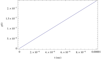
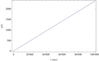
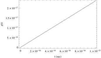
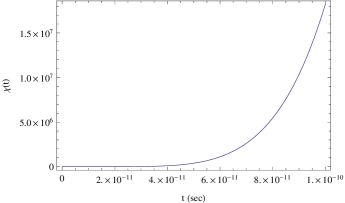
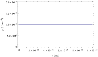
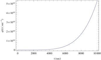
Also note that the present time in seconds is approximately $t_{p}\simeq 4.25\times 10^{17}$sec and also that $\kappa^{2}=8\pi G=2.0944\times 10^{-18}$GeV^-1, with $G$ denoting Newton’s constant. Using these, in Figs. 2 and 3, we present the time dependence of the scalar field $\chi$. As it is obvious, the scalar field $\chi$ is very small at early time, and remains small for a wide range of time, until present time where it grows large. After the present time era, it evolves larger and dominates the evolution. This qualitatively appealing behavior was also pointed out in noo3 , and we briefly address this issue in a later section.

Figure 3: The scalar field’s $\chi(t)$ evolution as a function of cosmic time $t$ with $c_{1}=10^{12}$, $c_{2}=10^{-20}$, $c_{3}=10^{10}$, $c_{4}=10^{-40}$, $t_{s}=10^{-35}$sec, $\alpha=4/3$ and for the initial conditions $\chi(0)\simeq 10^{-25}$, $\chi^{\prime}(0)\simeq 10$.

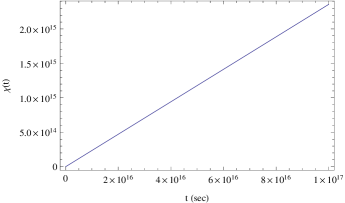
It is worth checking whether the inclusion of the $\varphi$-dependent potential term $\frac{6c_{1}c_{4}(t_{s}-\chi)^{\alpha}e^{-\kappa\sqrt{\frac{c_{3}}{2c_{1}}}\varphi}}{\kappa^{2}}$, in the scalar field $\chi$ potential results to a different behavior. In the most extreme case, the $\varphi$-dependent term will be of the form $\frac{6c_{1}c_{4}(t_{s}-\chi)^{\alpha}}{\kappa^{2}}$, which occurs if $\varphi$ is approximately equal to zero after inflation ends (assuming that our proposed mechanism ends inflation eventually). However, even including this term, the qualitative behavior remains the same, as it can be seen in Fig. 4, but the scalar field $\chi$ dominates to a great extent the evolution much more earlier in comparison to the other case.

Figure 4: The time dependence of the scalar field $\chi(t)$, with $c_{1}=10^{12}$, $c_{2}=10^{-20}$, $c_{3}=10^{10}$, $c_{4}=10^{-40}$, $t_{s}=10^{-35}$sec,$\alpha=4/3$ and for the initial conditions $\chi(0)\simeq 10^{-25}$, $\chi^{\prime}(0)\simeq 10$, including the $\varphi$-dependent term.

The same analysis can be performed for the kinetic function $\eta(\chi)$, which as we claimed previously, can be neglected at early times. Indeed, in Table 1, we have calculated the values of the kinetic function $\eta(\chi(t))$, for various time moments and also for the cases that the $\varphi$-dependent potential term is included (indicated by $\eta_{w}(\chi(t))$) or not (indicated by $\eta_{n}(\chi(t))$).

Time	$t\simeq 10^{-34}$	$t\simeq 10^{-15}$	$t\simeq 10^{-5}$	$t\simeq 10^{-4}$
$\eta(\chi_{n}(t))$	$3.48\times 10^{-13}$	$2.35\times 10^{-10}$	$4.110^{-7}$	$8.8\times 10^{-7}$
$\eta(\chi_{w}(t))$	$3.47\times 10^{-13}$	$2.2\times 10^{-10}$	$8.8\times 10^{11}$	$9.2\times 10^{13}$

Table 1: for the cases that the $\varphi$-dependent potential term is included (indicated by $\eta_{w}(\chi(t))$) or not (indicated by $\eta_{n}(\chi(t))$).

As it can be seen from Table (1), the behavior of the kinetic function is quite similar at early times in both cases, which are relevant for the inflationary era and in both cases the kinetic function is negligible and consequently the same applies for the kinetic term. The same analysis can be done for the potential of the scalar field $\chi(t)$, both for the cases that the $\varphi$-dependent term is kept in the potential or not. In Table 2, we present the values of the scalar field $\chi$ potential, with the $\varphi$-dependent term included in the potential (denoted as $\tilde{V}_{\chi}^{w}$) or not included (denoted as $\tilde{V}_{\chi}^{n}$).

Time	$t\simeq 10^{-34}$	$t\simeq 10^{-15}$	$t\simeq 10^{-5}$	$t\simeq 10^{-4}$
$\tilde{V}_{\chi}^{n}$	$1.5\times 10^{-13}$	$1.6\times 10^{-10}$	$3.5\times 10^{-7}$	$7.73\times 10^{-7}$
$\tilde{V}_{\chi}^{w}$	$3.46\times 10^{-13}$	$1.9\times 10^{-10}$	$8.8\times 10^{11}$	$9.2\times 10^{13}$

Table 2: The scalar field’s $\chi(t)$ scalar potential $\tilde{V}_{\chi}$ as a function of cosmic time $t$, with the $\varphi$-dependent term included in the potential (denoted as $\tilde{V}_{\chi}^{w}$) or not included (denoted as $\tilde{V}_{\chi}^{n}$)

As we can see in Table 2, the behavior of the potential for early times, in case that the $\varphi$-dependent term is included or not, is quite similar in both cases and also the potential is negligible at early times.

As a final task, we shall investigate the behavior of the potential (4), for the chosen values of the parameters (43). Since we assumed that the scalar field $\varphi$ does not evolve in a slow-roll way, it’s dynamical evolution is governed by the following non slow-roll equation of motion,

$$\ddot{\varphi}+3H\dot{\varphi}+\frac{\partial V(\varphi)}{\partial\varphi}=0\,,$$ (50)

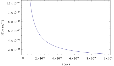
with $V(\varphi)$ given in Eq. (4) and notice that the difference between Eq. (50) and Eq. (25), is traced to the fact that the scalar field $\phi$ is non-canonical, while $\varphi$ is canonical. We solve numerically the dynamical evolution equation (50), and in Fig. 5, we plotted the behavior of the potential as a function of time, by choosing the initial conditions for the scalar field $\varphi$ to be $\varphi(0)=10^{20}$ (sec^-1), and $\varphi^{\prime}(0)=10^{-2}$ (sec^-2)

Figure 5: The time dependence of the scalar field potential $V(\varphi(t))$, with $c_{1}=10^{12}$, $c_{2}=10^{-20}$, $c_{3}=10^{10}$, $c_{4}=10^{-40}$, $t_{s}=10^{-35}$sec,$\alpha=4/3$ and for the initial conditions $\varphi(0)\simeq 10^{20}$ (sec^-1), $\varphi^{\prime}(0)\simeq 10^{-2}$ (sec^-2), including the $\varphi$-dependent term.

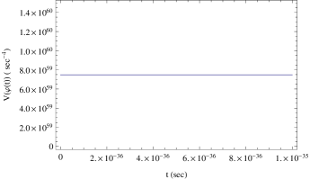
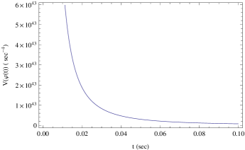
As it is obvious from Fig. 5, the scalar potential dominates at early times and also remains quite large until $t\simeq 10^{-1}$sec, from which point it rapidly decays, and therefore the second scalar field dominates the cosmological evolution. In order to see how rapid is the decay of the potential $V(\phi(t))$, in Table 3, we present some values of the scalar potential $V(\phi(t))$, for various time points. Notice that at $t=10^{-0.5}$sec, the potential decays quite rapidly and it is practically zero at $t=0$.

Time	$t\simeq 10^{-34}$	$t\simeq 10^{-1}$	$t\simeq 10^{-0.49}$	$t\simeq 10^{-0.48}$	$t\simeq 10^{-0.47}$
$V(\varphi(t))$	$7.4\times 10^{59}$	$8.5\times 10^{41}$	$2\times 10^{24}$	$516.3$	$4.5\times 10^{-39}$

Table 3: The scalar potential $V(\varphi(t))$ as a function of cosmic time $t$, for the initial conditions $\varphi(0)\simeq 10^{20}$ sec^-1, $\varphi^{\prime}(0)\simeq 10^{-2}$ sec^-2, and also with $c_{1}=10^{12}$, $c_{2}=10^{-20}$, $c_{3}=10^{10}$, $c_{4}=10^{-40}$, $t_{s}=10^{-35}$sec,$\alpha=4/3$.

An important remark is in order: The numerical analysis for the scalar field $\varphi$ evolution, showed that the scalar field $\varphi$ remains quite large for a wide range of time, therefore in the previous analysis of the scalar field evolution $\chi(t)$, the $\varphi$-dependent term can be safely neglected, since it is negligible ($\varphi\rightarrow\infty$). The behavior of the scalar field $\varphi(t)$ as a function of the cosmic time can be seen in Fig. 6.

Figure 6: The time dependence of the scalar field $\varphi(t)$, with $c_{1}=10^{12}$, $c_{2}=10^{-20}$, $c_{3}=10^{10}$, $c_{4}=10^{-40}$, $t_{s}=10^{-35}$sec,$\alpha=4/3$ and for the initial conditions $\varphi(0)\simeq 10^{20}$ (sec ^-1), $\varphi^{\prime}(0)\simeq 10$ (sec^-2).

Finally, we have to note that the results are quite model dependent and also strongly depend on the initial conditions and the values of the parameters. However, the focus in this paper was mainly to describe qualitatively the dynamical cosmological evolution and also to indicate that the system is dynamically unstable. This is the subject of the next section.

III Instability induced by Type IV singularity

Having described the qualitative behavior of the model, we come to the crucial part of our work, the instability of the system. As we demonstrated in the previous section, the two scalar field model with action (17) is described by the canonical scalar field action of Eq. (45), before and during the inflationary era, since the contribution of the second scalar field $\chi$ is negligible during this era. However, the dynamical cosmological evolution of the system is described by the Hubble rate (32). In practice, the parameters are chosen in such a way so that the term responsible for the singularity $\sim(-t+t_{s})^{\alpha}$, gives a very small contribution to the Hubble rate, which is mainly driven by the first term in (32). Since one of our main assumptions in this paper is that both scalar fields do not respect the slow-roll evolution requirements, we shall study the Hubble slow-roll parameters of Eq. (12), for the Hubble rate (32). A direct computation for the parameter $\epsilon_{H}$ yields,

$$\epsilon_{H}=\frac{\frac{c_{1}c_{3}}{(c_{2}+c_{3}t)^{2}}+c_{4}(-t+t_{s})^{-1+\alpha}\alpha}{\left(\frac{c_{1}}{c_{2}+c_{3}t}+c_{4}(-t+t_{s})^{\alpha}\right)^{2}},{\,},$$ (51)

while the parameter $\eta_{H}$ is equal to,

$$\eta_{H}=-\frac{\frac{2c_{1}c_{3}^{2}}{(c_{2}+c_{3}t)^{3}}+c_{4}(-t+t_{s})^{-2+\alpha}(-1+\alpha)\alpha}{2\left(\frac{c_{1}}{c_{2}+c_{3}t}+c_{4}(-t+t_{s})^{\alpha}\right)\left(-\frac{c_{1}c_{3}}{(c_{2}+c_{3}t)^{2}}-c_{4}(-t+t_{s})^{-1+\alpha}\alpha\right)}{\,}.$$ (52)

By looking Eq. (51), it is obvious that at early times, the contribution of the terms $c_{4}(-t+t_{s})^{-1+\alpha}\alpha$ and $c_{4}(-t+t_{s})^{\alpha}$ is negligible, compared to the other terms. We can also verify this numerically, since for $t=10^{-30}$sec, the term $c_{4}(-t+t_{s})^{-1+\alpha}\alpha$, is of the order $\sim 10^{-51}$, while the other term in the numerator of (51), namely $\frac{c_{1}c_{3}}{(c_{2}+c_{3}t)^{2}}$ is of the order $10^{62}$. Notice that we used the values for the parameters defined in Eq. (43). So practically we should neglect the aforementioned two terms at early times, and consequently the Hubble slow-roll parameter $\epsilon$ can be approximated by,

$$\epsilon_{H}\simeq\frac{\frac{c_{1}c_{3}}{(c_{2}+c_{3}t)^{2}}}{\left(\frac{c_{1}}{c_{2}+c_{3}t}\right)^{2}}=\frac{c_{3}}{c_{1}}{\,},$$ (53)

and by taking into account the identifications we made in Eq. (42), we obtain that the early time approximation of the Hubble slow-roll parameter $\epsilon_{H}$ for the Hubble rate (32) is $\epsilon_{H}\simeq\frac{1}{q}$, which is identical to the one we obtained in Eq. (13). Hence, this result also verifies our claim that the contribution of the slow-roll scalar $\chi$ at early times is practically zero. Notice also that at $t=t_{s}$, the Hubble slow-roll parameter is exactly $\epsilon=\frac{1}{q}$, without any approximation, since both the terms $c_{4}(-t+t_{s})^{-1+\alpha}\alpha$ and $c_{4}(-t+t_{s})^{\alpha}$, vanish, for the case of a Type IV singularity, which occurs for $\alpha>1$. Hence, although the Hubble slow-roll parameter $\epsilon$ is small and very well defined for a Type IV singularity, the same issue of the graceful exit from inflation persists, that is, inflation occurs, but never ends, the slow-roll parameter is constant.

III.0.1 Singular second Hubble slow-roll parameter and implications-Discussion on the results

Let us now investigate what happens with the second Hubble slow-roll parameter $\eta_{H}$, for the Hubble rate (32). As we can see in Eq. (52), in the case of a Type IV singularity at $t=t_{s}$, and when $1<\alpha<2$, the numerator of $\eta_{H}$ becomes divergent. This is very important, since this is an indication of instability in the exponential model. Moreover, the term responsible for the singularity, that is, $c_{4}(-t+t_{s})^{-2+\alpha}(-1+\alpha)\alpha$, is negligible for early cosmic times with $t>t_{s}$ and $t<t_{s}$, and only becomes important at exactly the singularity point $t=t_{s}$. The same applies for the corresponding term in the denominator, so at early times and for $t>t_{s}$ and for $t<t_{s}$, the second Hubble slow-roll parameter becomes, $\eta_{H}\simeq\frac{1}{q}$, but at $t=t_{s}$, $\eta_{H}\rightarrow\infty$. Recall that the second Hubble slow-roll parameter measures how long the inflationary era is.

So we have obtained a physically appealing resulting picture, according to which, at early times, the two field scalar model evolution is effectively identical to the one caused by a single scalar field with potential (4), and with slow-roll parameters that can be compatible with observations. In addition, the inflationary era ends violently at the point $t=t_{s}$ where a Type IV singularity occurs, at which point the second slow-roll parameter $\eta_{H}$ becomes divergent. Since the point $t_{s}$ can be arbitrarily chosen, this means that the inflationary evolution is unstable owing to this infinite singularity on the second Hubble slow-roll parameters at every point we may wish.

The critical question is, what does this instability indicates? Could it indicate somehow that this could be a possible mechanism for a graceful exit from inflation in this exponential scalar model? The quantitative answer to these questions is not a trivial task however, so we discuss here qualitatively, the implications of the instability and the possibility to connect the instability to the graceful exit solution.

This instability mechanism we propose for the ending of the inflationary era for the exponential model (4), is quite different in spirit in comparison to other existing mechanisms of ending of inflation, like tachyonic instabilities encyclopedia or via trace anomaly sergeitraceanomaly . Note that practically the singularity we found, indicates some instability of the dynamical cosmological system, but the qualitative description of this dynamical parameter $\eta_{H}$ is that it measures when inflation ends, and the singularity at $t=t_{s}$, definitely indicates strongly that the inflationary evolution is abruptly interrupted. So by having in mind that the only source of singularity is the second Hubble slow-roll index, it is rather tempting to ask if this instability could be actually indicate termination of the inflationary era. As we now demonstrate, this may be indeed occur.

In order to achieve this, we shall use the so-called slow-roll expansion, which is a generalization of the slow-roll approximation barrowslowroll . In fact, the slow-roll expansion is a more accurate approach towards finding the inflationary solution, in comparison to the standard slow-roll approach. The slow-roll expansion was introduced in barrowslowroll , and it is worth recalling in brief its basic features (for details see barrowslowroll ). Consider an inflationary solution that gives rise to a specific Hubble rate, $H(\varphi)$, where $\varphi$ is a canonical scalar field. Note that we shall for the moment adopt the notation of Ref. barrowslowroll , and we shall express all the quantities to be used as functions of the canonical scalar, and in the end we express all the parameters as functions of the cosmic time, implicitly through the variables $\epsilon_{H}$ and $\eta_{H}$. In the context of the Hubble slow-roll expansion, an attractor inflationary solution is assumed, to which all the solutions that can be obtained from the potential slow-roll approximation, tend asymptotically. Note that the attractor inflationary solution is very important for the analysis that follows. Then, the single scalar field Friedmann equation reads,

$$H^{2}(\varphi)=\frac{8\pi\kappa^{2}}{3}V(\varphi)\Big{(}1-\frac{1}{3}\epsilon_{H}(\varphi)\Big{)}^{-1}\,,$$ (54)

where $\epsilon_{H}$ is the Hubble slow-roll parameter appearing in (12), but expressed as a function of the scalar field $\varphi$. By using the binomial theorem, it is possible to obtain the following perturbative expansion barrowslowroll for the Friedmann equation (54),

$$H^{2}(\varphi)\simeq\frac{8\pi\kappa^{2}}{3}V(\varphi)\Big{(}1+\epsilon_{V}-\frac{4}{3}\epsilon_{V}^{2}+\frac{2}{3}\epsilon_{V}\eta_{V}$$ (55)

$$+\frac{32}{9}\epsilon_{V}^{3}+\frac{5}{9}\epsilon_{V}\eta_{V}^{2}-\frac{10}{3}\epsilon_{V}^{2}\eta_{V}+\frac{2}{9}\epsilon_{V}\xi^{2}_{V}+\mathcal{O}_{4}\Big{)}\,,$$

where we kept terms up to fourth order, and the parameters $\epsilon_{V},\eta_{V},\xi_{V}$ are defined in terms of the Hubble slow-roll parameters (12), as follows,

$$\eta_{V}=(3-\epsilon_{H})^{-1}\Big{(}3\epsilon_{H}+3\eta_{H}-\eta_{H}^{2}-\xi_{H}^{2}\Big{)},$$ (56)

$$\xi_{V}=(3-\epsilon_{H})^{-1}\Big{(}27\epsilon_{H}\eta_{H}+9\xi_{H}^{2}-9\epsilon_{H}\eta_{H}^{2}-12\eta_{H}\xi_{H}^{2}-3\sigma_{H}^{3}+3\eta_{H}^{2}\xi_{H}^{2}+\eta_{H}\sigma_{H}^{3}\Big{)}\,.$$

and also $\xi_{H}$ and $\sigma_{H}$ are given as functions of $\epsilon_{H}$ and $\eta_{H}$ below,

$$\xi_{H}^{2}=\epsilon_{H}\eta_{H}-\sqrt{\frac{1}{4\pi\kappa^{2}}}\sqrt{\epsilon_{H}}\eta_{H}^{\prime},\,\,\,\sigma_{H}^{3}=\xi_{H}^{2}(2\epsilon_{H}-\eta_{H})-\sqrt{\frac{1}{\kappa^{2}\pi}}\sqrt{\epsilon_{H}}\xi_{H}\xi_{H}^{\prime}\,.$$ (57)

Note that the prime denotes differentiation with respect to the scalar field $\varphi$ and also it is assumed that the solution $H(t)$ is the attractor of the theory. It is conceivable that the slow-roll approximation takes into account only the lowest order terms, while the expansion (55) provides a better approximation to the inflationary attractor $H(t)$, which continues to describe the inflationary era, until the slow-roll expansion breaks down. As was also stressed by the authors of barrowslowroll , the perturbative slow-roll expansion approximation breaks when the slow-roll parameters take large values, or if a singularity occurs. Using their example, for a potential of the form $\sim\varphi^{2}$, the expansion contains inverse powers of $\varphi$, and the inflationary era may end when the perturbative expansion is not valid anymore. This can occur definitely at the minimum of the potential at $\varphi=0$, where singularities appear in the expansion, but note that exit from inflation occurs earlier, owing to the fact that the expansion contains inverse powers of the scalar field $\varphi$.

The case we studied in this paper is perfectly described by what we just presented, that is, the exponential potential $\varphi$ drives the inflationary expansion until at some point a singularity occurs, so the solution is finally interrupted and the new attractor must be found. Practically this means that the inflationary attractor solution may be perfectly described by the perturbative slow-roll expansion solution, up to arbitrary order, until the perturbative expansion is violated, and the solutions exit from inflation. It is conceivable that the qualitative picture of our case goes as follows: The dynamical inflationary evolution is governed by the solution of the exponential scalar field, since the Type IV singular part of the Hubble rate (contribution of the second scalar), contributes very little to the dynamics. However, when the Type IV singularity time $t_{s}$ is reached, the second Hubble slow-roll parameter blows up and the expansion is not valid anymore, so this could indicate that inflation might end there.

Recall that the slow-roll expansion is constructed on the basic assumption that an attractor solution exists, before the exit from inflation. So as a final task, we shall prove that the solution $H(t)$, given in Eq. (32), can act as an attractor of the theory. Assuming that the attractor is,

$$H_{0}(t)=\frac{c_{1}}{c_{2}+c_{3}t}+c_{4}\left(t_{s}-t\right)^{\alpha}$$ (58)

and that the dynamics is governed by the canonical scalar field, we linearly perturb the system $H=H_{0}+\delta H$, so at first order we get barrowslowroll ,

$$-(\dot{H}_{0})^{2}\dot{\delta H}=48\pi\kappa^{4}H_{0}\delta H\,,$$ (59)

with the solution to the differential equation being of the following form,

$$\delta H=\delta H(t_{i})\exp\Big{(}-12\kappa^{2}\int_{t_{i}}^{t}\frac{H_{0}(t)}{(\dot{H}_{0}(t))^{2}}\Big{)}\,.$$ (60)

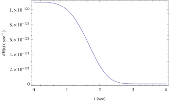
where $\delta H(t_{i})$, the value of the perturbation at some early time $t_{i}$. By choosing the values of the parameter we used in the previous sections, and also by choosing $\delta H(t_{i})$ to be very small, like for example $\delta H(t_{i})=10^{-120}$ ($sec^{-1}$), with $t_{i}=10^{-75}$sec, we can solve numerically the integral in Eq. (60). In Fig. 7, we plot the behavior of the perturbation $\delta H$ as a function of time, where can see that the perturbation vanishes eventually, in an exponential way. Note however that this may depend on the initial conditions at the initial time $t_{i}$, but the exponential decay is the resulting picture again. Hence, the solution (58), is the inflationary attractor of the theory, which is identical to the analytical expression that can result from the slow-roll expansion. However, at the Type IV singularity, the slow-roll expansion breaks down, and therefore this could indicate that the solution (58) is no longer the inflationary attractor. Recall again that there is a clear distinction between the slow-roll approximation and the slow-roll expansion. In the present case, the slow-roll expansion breaks down at second order.

Figure 7: The time dependence of the perturbation $\delta H(t)$, with $c_{1}=10^{12}$, $c_{2}=10^{-20}$, $c_{3}=10^{10}$, $c_{4}=10^{-40}$, $t_{s}=10^{-35}$sec,$\alpha=4/3$ and for the initial conditions $\delta H(10^{-75})=10^{-120}$ ($sec^{-1}$) .

Before closing this section, we need to note that if the singularity was Type III or even Type I, the Hubble slow-roll index $\epsilon_{H}$ would be singular at $t=t_{s}$, so practically we wouldn’t be able to even discuss about inflation, since the term $\sim(t-t_{s})^{\alpha-1}$, would make the Hubble slow-roll parameter $\epsilon_{H}$, quite large. In order to have a taste of how large, assume that $\alpha=-2$ (the Type I case according to our classification) then for $t\sim 10^{-30}$sec, this term would be of the order $10^{50}$, which is not negligible. Similar results hold true for the case of the Type III, and for the Type II singularity, but a full analysis is deferred to a future work, since this would require to change all the numerical values we assumed for the parameters and also we would have to change the initial conditions for the scalar fields.

In the next section with shall study the stability of the cosmological system of the two scalar fields when this is viewed as a dynamical system.

III.1 Cosmological dynamical system stability-Possible graceful exit from inflation via instabilities at the cost of phantom inflation

In this section we shall study the stability of the cosmological evolution caused by the two scalar fields, viewed as a dynamical system. Particularly, we shall be interested in the stability of the solution (20), which results from the reconstruction method we used for two scalar fields. The cosmological evolution is given in terms of the Hubble rate (32), and it is governed by the FRW equations of Eq. (18). In order to better study the system of cosmological equations as a dynamical system, we shall introduce the quantities $X_{\phi}$, $X_{\chi}$ and $\bar{Y}$, which are related to the scalar fields $\phi$ and $\chi$ as follows,

$$X_{\phi}=\dot{\phi}\,,\quad X_{\chi}=\dot{\chi}\,,\quad\bar{Y}=\frac{\tilde{f}(\phi,\chi)}{H}\,,$$ (61)

and in view of Eq. (61), the FRW equations (18) can be written as,

$$\frac{\mathrm{d}X_{\phi}}{\mathrm{d}N}=\frac{\omega^{\prime}(\phi)\left(X_{\phi}^{2}-1\right)}{2\omega(\phi)H}-3\left(X_{\phi}-\bar{Y}\right)$$

$$\frac{\mathrm{d}X_{\chi}}{\mathrm{d}N}=\frac{\eta^{\prime}(\chi)\left(X_{\chi}^{2}-1\right)}{2\eta(\chi)H}-3\left(X_{\chi}-\bar{Y}\right)$$

$$\frac{\mathrm{d}\bar{Y}}{\mathrm{d}N}=\frac{3X_{\phi}X_{\chi}\left(1-\bar{Y}^{2}\right)}{X_{\phi}+X_{\chi}}+\frac{\dot{H}}{H^{2}}\frac{X_{\phi}X_{\chi}+1-\bar{Y}(X_{\phi}+X_{\chi})}{X_{\phi}+X_{\chi}}\,.$$ (62)

Notice that the solution of Eq. (20), can be expressed in terms of the variables (61), as follows,

$$X_{\phi}=1\,,\quad X_{\chi}=1\,,\quad\bar{Y}=1\,.$$ (63)

By performing the following linear perturbations of the dynamical variables (61),

$$X_{\phi}=1+\delta X_{\phi}\,,\quad X_{\chi}=1+\delta X_{\chi}\,,\quad\bar{Y}=1+\delta\bar{Y}\,,$$ (64)

we obtain the following dynamical system which describes the evolution of the perturbations, namely,

$$\frac{\mathrm{d}}{\mathrm{d}N}\left(\begin{array}[]{c}\delta X_{\phi}\\ \delta X_{\chi}\\ \delta\bar{Y}\\ \end{array}\right)=\left(\begin{array}[]{ccc}-\frac{\omega^{\prime}(\phi)}{H\omega(\phi)}-3&0&3\\ 0&-\frac{\eta^{\prime}(\chi)}{H\eta(\chi)}-3&3\\ 0&0&-3-\frac{\dot{H}}{H^{2}}\\ \end{array}\right)\left(\begin{array}[]{c}\delta X_{\phi}\\ \delta X_{\chi}\\ \delta\bar{Y}\\ \end{array}\right)\,.$$ (65)

The eigenvalues corresponding to the matrix appearing in the dynamical system above, are equal to,

$$M_{\phi}=-\frac{\omega^{\prime}(\phi)}{H\omega(\phi)}-3\,,\quad{\,}M_{\chi}=-\frac{\eta^{\prime}(\chi)}{H\eta(\chi)}-3\,,\quad M_{\bar{Y}}=-3-\frac{\dot{H}}{H^{2}}\,.$$ (66)

Hence, by substituting the Hubble rate (32), we obtain,

$$M_{\phi}=-3-\frac{2c_{3}}{\left(\frac{c_{1}}{c_{2}+c_{3}t}+c_{4}(-t+t_{s})^{\alpha}\right)(c_{2}+c_{3}\phi)}\,,$$

$$M_{\chi}=-3-\frac{-1+\alpha}{\left(\frac{c_{1}}{c_{2}+c_{3}t}+c_{4}(-t+t_{s})^{\alpha}\right)(t_{s}-\chi)}\,,$$

$$M_{\bar{Y}}=-3+\frac{\frac{c_{1}c_{3}}{(c_{2}+c_{3}t)^{2}}+c_{4}(-t+t_{s})^{-1+\alpha}\alpha}{\left(\frac{c_{1}}{c_{2}+c_{3}t}+c_{4}(-t+t_{s})^{\alpha}\right)^{2}}\,,$$ (67)

From the theory of dynamical systems stability jost it is known that when all the eigenvalues are negative, the dynamical system is stable, so the evolution of perturbations (64) is stable. When one eigenvalue is positive and the other two negative, then the dynamical system is unstable, when two are positive and one negative, the system is stable, and when three eigenvalues are positive, then the dynamical system is unstable. Finally when one or more eigenvalues are zero, then we have a saddle point in the dynamical evolution of perturbations. As it is clear from Eq. (III.1), for the choice of the parameters as in Eq. (43) both $M_{\phi}$ and $M_{\bar{Y}}$ are negative, but for the eigenvalue $M_{\chi}$, it is always positive, if the value of $\chi(t)$ is larger from $t_{s}$. This however strongly depends on the initial conditions for the field $\chi(t)$. For the initial conditions we chose (44) in the previous sections, this is always true since $\chi(0)=10^{-25}$, and the scalar field $\chi(t)$ increases with time, as we evinced in a previous section. Therefore, in our case the dynamical system always develops an instability, with this feature probably indicating that the inflationary solution driven by the scalar field $\varphi$ at early times is not the final attractor of the system, at least for the initial conditions we chose. However, the full study of the cosmological dynamical system exceeds the purposes of this paper, since our aim is to qualitatively stress the fact that, the Type IV singularity in some way makes the system unstable and the inflationary solution of the system at early times is not the final attractor of the system.

Finally, we should note that if the initial conditions of the scalar field $\chi(t)$, were chosen to be smaller than the value of $t_{s}$, or if in our case $t_{s}$ is chosen to be larger than $10^{-25}$, so that $\chi(0)<t_{s}$, then it is possible that, as $\chi$ increases, at some point $t_{1}$ corresponding to the crossing point $t_{s}=\chi(t_{1})$, the eigenvalue $M_{\chi}$ becomes infinite. This infinity may also indicate an instability of the dynamical system, thus indicating an abrupt change of the final attractor solution of the scalar field $\varphi$. From a mathematical point of view, this dynamical system analysis is a difficult issue and should be scrutinized in order to come to rigid conclusions. From this brief study we keep only the result that the dynamical system of perturbations of the cosmological parameters $X_{\phi}$, $X_{\chi}$ and $\bar{Y}$, is unstable.

IV Late-time evolution of the two scalar field model

In the previous sections we thoroughly studied the early time behavior of the two scalar field model, but we did not address the late-time evolution study of the model. Here we study the late-time behavior of the two scalar model, in terms of the effective equation of state (EoS) of the model. Before getting into the detailed analysis, let us recall the essential features of the two scalar field model we used, assuming that the parameters are as these appear in Eq. (43). Firstly, we assumed that the Type IV singularity occurs at early times, specifically at $t=t_{s}$, and secondly, the two scalar fields are required not to obey the slow-roll conditions. As we evinced, for the choice of the variables as in Eq. (43) and also by assuming that the initial conditions of the scalar field $\chi$ are taken as in Eq. (44), we demonstrated that the scalar field $\chi$ has a negligible contribution to the cosmological evolution of the model at early times, but dominates the cosmological evolution at late times. As we now show, this behavior can also be seen by studying the EoS of the two scalars system. The EoS parameter $w_{eff}$ for the two scalar model is given by,

$$w_{\mathrm{eff}}=\frac{p}{\rho}=-1-\frac{2\dot{H}}{3H^{2}}\,.$$ (68)

By using the form of the Hubble rate given in Eq. (32), the EoS reads,

$$w_{\mathrm{eff}}=-1-\frac{2\left(-\frac{c_{1}c_{3}}{(c_{2}+c_{3}t)^{2}}-c_{4}(-t+t_{s})^{-1+\alpha}\alpha\right)}{3\left(\frac{c_{1}}{c_{2}+c_{3}t}+c_{4}(-t+t_{s})^{\alpha}\right)^{2}}\,.$$ (69)

The above relation (69) will be the starting point of our analysis. We shall investigate the behavior of the EoS at early and at late times. We start off with early time, in which case, the contribution of the terms $\sim c_{4}(-t+t_{s})^{-1+\alpha}\alpha$ and $c_{4}(-t+t_{s})^{\alpha}$ appearing in the numerator and the denominator of the fraction in Eq. (69), is negligible compared to the other terms. Also, when $t\simeq t_{s}$, these are identically zero, for the value of the parameter $\alpha$ we chose. Therefore, by neglecting these, the EoS at early times reads,

$$w_{\mathrm{eff}}\simeq-1+\frac{2c_{3}}{3c_{1}}\,,$$ (70)

which clearly describes quintessential acceleration, different from de Sitter though, since in our case $\frac{c_{3}}{c_{1}}=\frac{1}{q}$ (see Eq. (42)) and we took $q=100$, so it cannot be considered nearly de Sitter, but purely quintessential acceleration. Hence the inflationary era is a quintessence era, without the possibility of evolving into a phantom evolution. With regards to the late-time era, it is conceivable that as $t$ grows larger, approaching the present time era $t_{p}\simeq 4.25\times 10^{17}$sec, the terms $\sim c_{4}(-t+t_{s})^{-1+\alpha}\alpha$ and $c_{4}(-t+t_{s})^{\alpha}$ will start to dominate the evolution, therefore the EoS at late-time reads,

$$w_{\mathrm{eff}}\simeq-1+\frac{2(-t+t_{s})^{-1-\alpha}\alpha}{3c_{4}}\,,$$ (71)

and since $\alpha=4/3$ and also $t_{s}\ll t$, then,

$$(-t+t_{s})^{\alpha-1}\simeq(-t)^{\alpha-1}=-t^{\alpha-1}\,.$$ (72)

Consequently, the EoS (71) becomes at late times,

$$w_{\mathrm{eff}}\simeq-1-\frac{2t^{-1-\alpha}\alpha}{3c_{4}}\,.$$ (73)

The EoS (73) describes nearly phantom acceleration, with nearly meaning that the acceleration is slightly phantom. Indeed, since we chose $c_{4}=10^{-40}$, and also owing to the fact that we consider late times, when $t$ is of the order of the present time, that is $t\simeq 4\times 10^{17}$sec, then the EoS is approximately equal to $w_{\mathrm{eff}}\simeq-1.06545$. Note that observations indicate that the EoS at present time or in near future may crossed the phantom divide phantom , so this result is quite interesting.

In conclusion, in the context of the two scalar field model that realizes a Type IV singularity at early times, we were able to describe early and late-time acceleration in a unified way, by using the same theoretical framework. One interesting scenario that we did not address here is to study what is the impact on the two scalar field model we used, if the Type IV singularity occurs at late-time. However, this would require to change completely the constraints we used, so we hope to address this in the future.

V Type IV singularity as a source of instability for other scalar models-Universal description for non-slow-roll evolution

From all the previous sections it is conceivable that the instability in scalar models caused by a Type IV singularity, can be achieved if the slow-roll conditions for the scalar fields are not taken into account. Then, it is possible that the Hubble slow-roll parameters are small during the inflationary era, but these blow-up at the Type IV singularity, where inflation is abruptly interrupted. So by saying that the slow-roll condition is not taken into account, it is meant that the indicators for the inflationary dynamics are not the potential slow-roll parameters barrowslowroll , but the Hubble slow-roll parameters barrowslowroll . In this section we briefly investigate if this instability mechanism we proposed in this paper, can also generate have implications on other scalar models if these are put into proper context. We shall study two quite popular scalar models, a large field inflation model encyclopedia ; noo1 and a modified $R^{2}$ inflation model encyclopedia ; noo3 . We start off with the large field inflation model, which we studied in detail in noo1 and we were able to associate it to a Type IV singular evolution, by using a single scalar field and not two. Let us recall the essential information for the Type IV singular evolution for the large field inflation and for details the reader is referred to noo1 . The Hubble rate that describes the Type IV singular evolution is equal to,

$$H(t)=f_{0}\left(t_{s}-t\right)^{\alpha}\,,$$ (74)

so for $\alpha>1$ a Type IV singularity occurs. Consider the single scalar field action,

$$S=\int d^{4}x\sqrt{-g}\left\{\frac{1}{2\kappa^{2}}R-\frac{1}{2}\omega(\phi)\partial_{\mu}\phi\partial^{\mu}\phi-V(\phi)+L_{\mathrm{matter}}\right\}\,.$$ (75)

where the function $\omega(\phi)$ stands for the kinetic function and $V(\phi)$ is the scalar potential of the scalar field $\phi$. Using Eq. (75), the effective energy density and the effective pressure of the non-canonical scalar field $\phi$ can be written,

$$\rho=\frac{1}{2}\omega(\phi){\dot{\phi}}^{2}+V(\phi)\,,\quad p=\frac{1}{2}\omega(\phi){\dot{\phi}}^{2}-V(\phi)\,.$$ (76)

Then in view of Eq. (76) the scalar potential $V(\phi)$ and the kinetic function $\omega(\phi)$ can be expressed in terms of the Hubble rate as follows,

$$\omega(\phi){\dot{\phi}}^{2}=-\frac{2}{\kappa^{2}}\dot{H}\,,\quad V(\phi)=\frac{1}{\kappa^{2}}\left(3H^{2}+\dot{H}\right)\,.$$ (77)

The single scalar field reconstruction method is based on the crucial assumption that the kinetic function $\omega(\phi)$ and the scalar potential $V(\phi)$, can be expressed as functions of a single function $f(\phi)$, as follows,

$$\omega(\phi)=-\frac{2}{\kappa^{2}}f^{\prime}(\phi)\,,\quad V(\phi)=\frac{1}{\kappa^{2}}\left(3f(\phi)^{2}+f^{\prime}(\phi)\right)\,.$$ (78)

For further details on this method, see Nojiri:2005sx ; noo1 . Consequently, the FRW equations for the single scalar read Nojiri:2005sx ; noo1 ,

$$\phi=t\,,\quad H=f(t)\,.$$ (79)

The kinetic function and scalar potential for the scalar $\phi$, in the case that the Hubble rate is given as in (74), near $t=t_{s}$, are equal to,

$$\omega(\phi)=\frac{2\alpha f_{0}}{\kappa^{2}}\left(t_{s}-\phi\right)^{\alpha-1}\,,\quad V(\phi)\sim-\frac{\alpha f_{0}}{\kappa^{2}}\left(t_{s}-\phi\right)^{\alpha-1}\,,$$ (80)

By canonically transforming the single scalar field $\phi$ (see also appendix), we can have the potential in the following form,

$$V(\varphi)\sim-\frac{\alpha f_{0}}{\kappa^{2}}\left\{-\frac{\kappa\left(\alpha+1\right)}{2\sqrt{2\alpha f_{0}}}\varphi\right\}^{\frac{2\left(\alpha-1\right)}{\alpha+1}}\,,$$ (81)

where the field $\varphi$ is canonical. The potential (81), is known to describe large field inflation Barrow:2015ora ; encyclopedia . The observational implications of the potential (81), are quite appealing as we evinced in noo1 , in the case that the singularity occurs at the end or after inflation, but in the context of a slow-roll evolution. Now consider that we abandon the slow-roll evolution requirement and in addition assume that the singularity can occur at an arbitrary time instance. The Hubble slow-roll parameters for the Hubble rate (74), are equal to,

$$\epsilon_{H}=\frac{(-t+t_{s})^{-1-\alpha}\alpha}{f_{0}},{\,}{\,}{\,}\eta_{H}=\frac{(-t+t_{s})^{-1-\alpha}(-1+\alpha)}{2f_{0}}{\,}.$$ (82)

Therefore by choosing $f_{0}$ to be enormously large, larger than $(-t+t_{s})^{-1-\alpha}$, that is, $f_{0}\gg(-t+t_{s})^{-1-\alpha}$, for $t\simeq t_{s}$, then both the Hubble slow-roll parameters $\epsilon_{H}$ and $\eta_{H}$ can be significantly smaller than unity, $\epsilon_{H},\eta_{H}\ll 1$, in the neighborhood of $t\sim t_{s}$. But for a Type IV singularity ($\alpha>1$), both the Hubble slow-roll parameters blow up to infinity at $t=t_{s}$, where the singularity occurs. Therefore, even in the non-slow-roll approximation, this could be an indication that inflation is interrupted severely due to the existence of an singular instability. Hence, our mechanism can work for other potentials too, apart from the exponential we explored in the previous sections. Notice that $f_{0}$ is a free parameter, so it can be chosen appropriately in order concordance with Planck data can be achieved, at least in the neighborhood of the Type IV singularity where inflation can be chosen to end.

Before closing, we demonstrate in brief that the same mechanism can create grateful exit from inflation for nearly $R^{2}$ potentials which can generate a singular evolution, which we studied in noo3 . As we evinced in noo3 , the Hubble rate for the Type singularity generating nearly $R^{2}$ potentials reads,

$$H(t)=\frac{c_{1}}{c_{2}+c_{3}t}+c_{4}+c_{5}\left(t_{s}-t\right)^{\alpha}\,,$$ (83)

and consequently, the first Hubble slow-roll parameter $\epsilon_{H}$ is equal to,

$$\epsilon_{H}=-\frac{-\frac{c_{1}c_{3}}{(c_{2}+c_{3}t)^{2}}-c_{5}(-t+t_{s})^{-1+\alpha}\alpha}{\left(c_{4}+\frac{c_{1}}{c_{2}+c_{3}t}+c_{5}(-t+t_{s})^{\alpha}\right)^{2}}{\,},$$ (84)

while the parameter $\eta_{H}$ is equal to,

$$\eta_{H}=-\frac{\frac{2c_{1}c_{3}^{2}}{(c_{2}+c_{3}t)^{3}}+c_{5}(-t+t_{s})^{-2+\alpha}(-1+\alpha)\alpha}{2\left(c_{4}+\frac{c_{1}}{c_{2}+c_{3}t}+c_{5}(-t+t_{s})^{\alpha}\right)\left(-\frac{c_{1}c_{3}}{(c_{2}+c_{3}t)^{2}}-c_{5}(-t+t_{s})^{-1+\alpha}\alpha\right)}{\,}.$$ (85)

Hence, for $1<\alpha<2$, the second slow-roll parameter blows up at the Type IV singularity. Therefore, in this case too, the Type IV singularity induced instability can work in the same way as in the exponential model we studied in the previous sections. Note that the model studied in noo3 and the one we studied in this paper have many qualitative similarities, except that in noo3 we used the slow-roll approximation for the canonical scalar $\varphi$.

VI Concluding remarks

In this paper we included a Type IV singularity in the dynamical evolution of a quite well studied exponential scalar model, which is known to be compatible with the Planck data, when the spectral index of primordial perturbations is considered. In order to successfully incorporate the Type IV singularity we used two scalar fields, and by employing very well known scalar reconstruction techniques, we managed to produce the Type IV singular behavior appearing in the Hubble rate of the model. The scalar exponential model we studied however, is known to suffer from the graceful exit from inflation problem, but in the context of our model, we provided an indication on how inflation might end in this model. However, this issue has to be thoroughly addressed, a task which is beyond the scopes of this introductory paper on these issues.

In order to generate an instability, we assumed that both the scalar fields, one being canonical and one non-canonical, do not satisfy the slow-roll requirements. Also, the values of the parameters and the initial conditions on the fields are chosen in such a way, so that the model exhibits the following features:

• The Type IV is assumed to occur at early times. In the context of our model, this will indicate the end of inflation in the model.

• At early times, the canonical scalar, which is the one that corresponds to the exponential scalar model, dominates the cosmological evolution, with the scalar potential and kinetic term of the non-canonical field being neglected. Special emphasis was given on the inflationary era.

• The non-canonical scalar never becomes a phantom scalar, so singular phantom evolution is avoided.

As a side effect of our model, the late-time evolution is governed by the non-canonical scalar, as we analyzed in detail. In fact, in the context of our model, late-time acceleration and early-time acceleration can be described in a unified way, as we evinced.

For our two scalar field model, since the slow-roll condition is not respected by both scalar fields, the indicators that determine the inflationary process, if it occurs and when it ends, are the Hubble slow-roll parameters. By calculating these for a Type IV singularity, we obtained the quite appealing result that at the Type IV singularity, the second Hubble slow-roll parameter, which is known to indicate the end of inflation, diverges at the Type IV singularity. As we claimed, this might be an indication that inflation ends at the point of the Type IV singularity. Away from the singularity however, and always referring to early times, the Hubble slow-roll indices are approximately (and in some cases exactly) equal to the ones corresponding to the exponential scalar model solely. This in some way also validates our claims about the evolution of the two scalar field system. In addition, we supported numerically and verified in a semi-quantitative way our theoretical claims. We need to note though that in order to obtain some quantitative results, the analysis must be much more rigid and also someone should examine the dynamical system of the cosmological equations exactly. Our aim was to indicate in a qualitative and semi-quantitative way, the fact that a Type IV singularity might be responsible for the graceful exit from inflation, to certain cosmological models. Finally, we studied analytically the stability of the cosmological equations, when these are viewed as a dynamical system, by examining the dynamical system of linear perturbations of certain parameters, related to some physical quantities. As we demonstrated, the system is unstable, with this instability possibly indicating the fact that the initial solution corresponding to the canonical scalar field is not an attractor of the dynamical system. Indeed, this was the case, since the solution lasts up to the point that the Type IV singularity occurs, with the duration of the solution being quantified by the second Hubble slow-roll parameter.

We need to note that the effects of the Type IV singularity on the cosmological evolution of the model are somehow unique since only the second slow-roll parameter diverges and not the first. One should however examine the rest of finite time singularities, with the most appealing, from a phenomenological point of view, being the Type II. Since finite time singularities frequently occur in cosmology, the phenomenological implications of these have to be understood in detail, especially the effects of the mildest ones, like the Type IV and Type II. These could be the link between a quantum theory of cosmology and the classical cosmological theory, with the most appealing candidate of a quantum cosmology theory being Loop Quantum Cosmology LQC . Finally, it is worth to study the evolution of the model we studied in this paper, in the context of theories with generalized equation of state. For a recent study see fin .

Appendix

Here we discuss in brief why the incorporation of the Type IV singularity in the cosmological evolution of a single scalar field is very difficult, not to say impossible. Consider the following generic non-canonical scalar field action,

$$S=\int d^{4}x\sqrt{-g}\left\{\frac{1}{2\kappa^{2}}R-\frac{1}{2}\omega(\phi)\partial_{\mu}\phi\partial^{\mu}\phi-V(\phi)\right\}\,.$$ (86)

with the function $\omega(\phi)$ being the kinetic function and the scalar potential is $V(\phi)$. For the flat FRW background of Eq. (1), the energy density and the corresponding pressure are equal to,

$$\rho=\frac{1}{2}\omega(\phi){\dot{\phi}}^{2}+V(\phi)\,,\quad p=\frac{1}{2}\omega(\phi){\dot{\phi}}^{2}-V(\phi)\,.$$ (87)

Therefore, the potential $V(\phi)$ and the kinetic function $\omega(\phi)$ can be expressed in terms of the Hubble rate in the following way,

$$\omega(\phi){\dot{\phi}}^{2}=-\frac{2}{\kappa^{2}}\dot{H}\,,\quad V(\phi)=\frac{1}{\kappa^{2}}\left(3H^{2}+\dot{H}\right)\,.$$ (88)

By making the transformation (37), we can rewrite the action of Eq. (86), in terms of the canonical scalar field $\varphi$, since the kinetic term becomes,

$$-\omega(\phi)\partial_{\mu}\phi\partial^{\mu}\phi=-\partial_{\mu}\varphi\partial^{\mu}\varphi\,.$$ (89)

and finally the action of Eq. (86) reads,

$$S=\int d^{4}x\sqrt{-g}\left\{\frac{1}{2\kappa^{2}}R-\frac{1}{2}\partial_{\mu}\varphi\partial^{\mu}\varphi-V(\varphi)\right\}\,.$$ (90)

The technique that simplifies to a great extent the incorporation of finite time singularities, is the scalar-reconstruction technique developed in Refs. Nojiri:2005pu ; Capozziello:2005tf , which is based on the assumption that the kinetic function and the scalar potential can be written in terms of a function $f(\phi)$, in the following way,

$$\omega(\phi)=-\frac{2}{\kappa^{2}}f^{\prime}(\phi)\,,\quad V(\phi)=\frac{1}{\kappa^{2}}\left(3f(\phi)^{2}+f^{\prime}(\phi)\right)\,,$$ (91)

Therefore, if we assume that no other matter fluids are present in the cosmological equations, the field equations (87) take the following form,

$$\phi=t\,,\quad H=f(t)\,.$$ (92)

As in the $R^{2}$ inflation case, which we studied in noo3 , our inability to incorporate the finite time singularity for the potential (4), is traced on the fact that the potential has an exponential functional dependence with respect to the scalar field $\varphi$. In the case of a Type IV singularity, a quite general form of the function $f(t)$ that can describe the Type IV singular evolution, has the form,

$$f(t)=c(t-t_{s})^{b}+f_{1}(t)$$ (93)

with $f_{1}(t)$ being the non-canonical scalar-tensor reconstruction function that produces the scalar potential (4). Equivalently, $f(t)$ can be equal to,

$$f(t)=f_{1}(t)(t-t_{s})^{b},{\,}{\,}{\,}f(t)=e^{(t-t_{s})^{\alpha}}+c$$ (94)

with $c$ being an arbitrary constant. For both the cases (93) and (94), it is very difficult to incorporate the Type IV singularity for the following reasons:

• The function $f(t)$ must be chosen in such a way, so that it is possible to solve the integral $\varphi=\int^{\phi}\sqrt{f^{\prime}(\phi)}\mathrm{d}\phi$, in terms of $\phi=\phi(\varphi)$. This is not so easy to be done for the functions $f(t)$ of Eqs. (93) and (94).

• In the case that an ansatz is found and the function $f(\phi)$ is found, so that $\phi=\phi(\varphi)$ can be explicitly solved, then even in this case, the resulting scalar potential becomes severely constrained and the potential (4) cannot be easily reproduced even in parts. In order to see this, suppose that $\phi(\varphi)$ is found in explicit form, then the corresponding scalar potential $V(\phi(\varphi))$ would be equal to,

  $$V(\phi(\varphi))=\frac{1}{\kappa^{2}}\left(3f(\phi(\varphi))^{2}+f^{\prime}(\phi(\varphi))\right)\,,$$ (95)

  and this potential must be of the following form,

  $$V(\phi(\varphi))=V_{0}e^{-\sqrt{\frac{2}{q}}\kappa\varphi}+V_{1}(\phi(\varphi))$$ (96)

  which is a rather formidable task to do, since an ansatz is needed. Work is in progress though to find such an ansatz.

References

- (1) J. D. Barrow, G. J. Galloway and F. J. Tipler, Mon. Not. Roy. Astron. Soc. 223 (1986) 835.
- (2) J. D. Barrow, Class. Quant. Grav. 21 (2004) L79 [gr-qc/0403084]. ; J. D. Barrow, Class. Quant. Grav. 21 (2004) 5619 [gr-qc/0409062].
-
(3)
S. Nojiri and S. D. Odintsov,
Phys. Lett. B 595 (2004) 1
[hep-th/0405078];
Z. Keresztes, L. Á. Gergely, A. Y. Kamenshchik, V. Gorini and D. Polarski, Phys. Rev. D 88 (2013) 023535 [arXiv:1304.6355 [gr-qc]];
M. Bouhmadi-Lopez, C. Kiefer, B. Sandhofer and P. V. Moniz, Phys. Rev. D 79, 124035 (2009) [arXiv:0905.2421 [gr-qc]];
V. Sahni and Y. Shtanov, JCAP 0311, 014 (2003) [arXiv:astro-ph/0202346];
K. Lake, Class. Quant. Grav. 21, L129 (2004) [arXiv:gr-qc/0407107];
J. D. Barrow and C. G. Tsagas, Class. Quant. Grav. 22, 1563 (2005) [arXiv:gr-qc/0411045];
M. P. Dabrowski, Phys. Rev. D 71, 103505 (2005) [arXiv:gr-qc/0410033];
Phys. Lett. B 625, 184 (2005); L. Fernandez-Jambrina and R. Lazkoz, Phys. Rev. D 70, 121503 (2004) [arXiv:gr-qc/0410124]; Phys. Rev. D 74, 064030 (2006) [arXiv:gr-qc/0607073]; arXiv:0805.2284 [gr-qc];
P. Tretyakov, A. Toporensky, Y. Shtanov and V. Sahni, Class. Quant. Grav. 23, 3259 (2006) [arXiv:gr-qc/0510104];
H. Stefancic, Phys. Rev. D 71, 084024 (2005) [arXiv:astro-ph/0411630];
A. V. Yurov, A. V. Astashenok and P. F. Gonzalez-Diaz, Grav. Cosmol. 14, 205 (2008) [arXiv:0705.4108 [astro-ph]];
K. Bamba, S. D. Odintsov, L. Sebastiani and S. Zerbini, Eur. Phys. J. C 67 (2010) 295 [arXiv:0911.4390 [hep-th]];
I. Brevik and O. Gorbunova, Eur. Phys. J. C 56, 425 (2008) [arXiv:0806.1399 [gr-qc]];
K. Bamba, S. Nojiri and S. D. Odintsov, JCAP 0810 (2008) 045 [arXiv:0807.2575 [hep-th]].;
M. Bouhmadi-Lopez, P. F. Gonzalez-Diaz and P. Martin-Moruno, Phys. Lett. B 659, 1 (2008) [arXiv:gr-qc/0612135]; arXiv:0707.2390 [gr-qc];
C. Cattoen and M. Visser, Class. Quant. Grav. 22, 4913 (2005) [arXiv:gr-qc/0508045];
J. D. Barrow and S. Z. W. Lip, arXiv:0901.1626 [gr-qc];
M. Bouhmadi-Lopez, Y. Tavakoli and P. V. Moniz, arXiv:0911.1428 [gr-qc].;
J. D. Barrow, A. B. Batista, J. C. Fabris, M. J. S. Houndjo and G. Dito, Phys. Rev. D 84 (2011) 123518 [arXiv:1110.1321 [gr-qc]];
J. D. Barrow, S. Cotsakis and A. Tsokaros, Class. Quant. Grav. 27 (2010) 165017 [arXiv:1004.2681 [gr-qc];
S. Cotsakis and I. Klaoudatou, J. Geom. Phys. 55, 306 (2005) [arXiv:gr-qc/0409022] - (4) J. D. Barrow and A. A. H. Graham, Phys. Rev. D 91, no. 8, 083513 (2015) [arXiv:1501.04090 [gr-qc]].
- (5) S. Nojiri, S. D. Odintsov and S. Tsujikawa, Phys. Rev. D 71, 063004 (2005) [arXiv:hep-th/0501025].
(6)
R. R. Caldwell, M. Kamionkowski and N. N. Weinberg,
Phys. Rev. Lett. 91, 071301 (2003)
[arXiv:astro-ph/0302506].;
B. McInnes, JHEP 0208 (2002) 029 [arXiv:hep-th/0112066];
S. Nojiri and S. D. Odintsov, Phys. Lett. B 562, 147 (2003) [arXiv:hep-th/0303117];
S. Nojiri and S. D. Odintsov, Phys. Rev. D 72 (2005) 023003 [hep-th/0505215];
V. Gorini, A. Kamenshchik and U. Moschella, Phys. Rev. D 67 (2003) 063509 [astro-ph/0209395];
E. Elizalde, S. Nojiri and S. D. Odintsov, Phys. Rev. D 70 (2004) 043539 [hep-th/0405034]. ;
V. Faraoni, Int. J. Mod. Phys. D 11, 471 (2002) [arXiv:astro-ph/0110067];
P. Singh, M. Sami and N. Dadhich, Phys. Rev. D 68, 023522 (2003) [arXiv:hep-th/0305110];
S. Nojiri and S. D. Odintsov, Phys. Rev. D 70 (2004) 103522 [hep-th/0408170].;
C. Csaki, N. Kaloper and J. Terning, Annals Phys. 317, 410 (2005) [arXiv:astro-ph/0409596];
P. X. Wu and H. W. Yu, Nucl. Phys. B 727, 355 (2005) [arXiv:astro-ph/0407424];
S. Nesseris and L. Perivolaropoulos, Phys. Rev. D 70, 123529 (2004) [arXiv:astro-ph/0410309];
M. Sami and A. Toporensky, Mod. Phys. Lett. A 19, 1509 (2004) [arXiv:gr-qc/0312009];
H. Stefancic, Phys. Lett. B 586, 5 (2004) [arXiv:astro-ph/0310904];
L. P. Chimento and R. Lazkoz, Phys. Rev. Lett. 91, 211301 (2003) [arXiv:gr-qc/0307111];
Mod. Phys. Lett. A 19, 2479 (2004) [arXiv:gr-qc/0405020];
J. G. Hao and X. Z. Li, Phys. Lett. B 606, 7 (2005) [arXiv:astro-ph/0404154];
E. Babichev, V. Dokuchaev and Yu. Eroshenko, Class. Quant. Grav. 22, 143 (2005) [arXiv:astro-ph/0407190];
X. F. Zhang, H. Li, Y. S. Piao and X. M. Zhang, Mod. Phys. Lett. A 21, 231 (2006) [arXiv:astro-ph/0501652];
E. Elizalde, S. Nojiri, S. D. Odintsov and P. Wang, Phys. Rev. D 71, 103504 (2005) [arXiv:hep-th/0502082];
M. P. Dabrowski and T. Stachowiak, Annals Phys. 321, 771 (2006) [arXiv:hep-th/0411199];
F. S. N. Lobo, Phys. Rev. D 71, 084011 (2005) [arXiv:gr-qc/0502099];
R. G. Cai, H. S. Zhang and A. Wang, Commun. Theor. Phys. 44, 948 (2005) [arXiv:hep-th/0505186];
I. Y. Aref’eva, A. S. Koshelev and S. Y. Vernov, Theor. Math. Phys. 148, 895 (2006) [Teor. Mat. Fiz. 148, 23 (2006)] [arXiv:astro-ph/0412619];
Phys. Rev. D 72, 064017 (2005) [arXiv:astro-ph/0507067];
H. Q. Lu, Z. G. Huang and W. Fang, arXiv:hep-th/0504038;
W. Godlowski and M. Szydlowski, Phys. Lett. B 623, 10 (2005) [arXiv:astro-ph/0507322];
J. Sola and H. Stefancic, Phys. Lett. B 624, 147 (2005) [arXiv:astro-ph/0505133];
B. Guberina, R. Horvat and H. Nikolic, Phys. Rev. D 72, 125011 (2005) [arXiv:astro-ph/0507666];
M. P. Dabrowski, C. Kiefer and B. Sandhofer, Phys. Rev. D 74, 044022 (2006) [arXiv:hep-th/0605229];
- (7) E. Elizalde, S. Nojiri, S. D. Odintsov, D. Saez-Gomez and V. Faraoni, Phys. Rev. D 77 (2008) 106005 [arXiv:0803.1311 [hep-th]].
- (8) S. W. Hawking and R. Penrose, Proc. Roy. Soc. Lond. A 314 (1970) 529.
- (9) K. S. Virbhadra, S. Jhingan and P. S. Joshi, Int. J. Mod. Phys. D 6 (1997) 357 [gr-qc/9512030].
- (10) K. S. Virbhadra, Phys. Rev. D 60 (1999) 104041 [gr-qc/9809077].
- (11) K. S. Virbhadra and G. F. R. Ellis, Phys. Rev. D 65 (2002) 103004.
(12)
G. F. R. Ellis, J. Murugan and C. G. Tsagas,
Class. Quant. Grav. 21 (2004) 233
[gr-qc/0307112];
G. F. R. Ellis and R. Maartens, Class. Quant. Grav. 21 (2004) 223 [gr-qc/0211082]. -
(13)
M. Novello, S.E.Perez Bergliaffa, Phys.Rept. 463 (2008) 127 [arXiv:0802.1634];
C. Li, R. H. Brandenberger and Y. K. E. Cheung, Phys. Rev. D 90 (2014) 12, 123535 [arXiv:1403.5625 [gr-qc]].;
Yi-Fu Cai, E. McDonough, F. Duplessis, R. H. Brandenberger, JCAP 1310 (2013) 024 [arXiv:1305.5259];
Yi-Fu Cai, E. Wilson-Ewing, JCAP 1403 (2014) 026 [arXiv:1402.3009 ];
J. Haro, J. Amoros, JCAP 08(2014)025 [arXiv:1403.6396 ];
A. Nicolis, R. Rattazzi, E. Trincherini, Phys.Rev. D 79 (2009) 064036 [arXiv:0811.2197];
C. Deffayet , G. Esposito-Farese (Paris, Inst. Astrophys.), A. Vikman, Phys.Rev. D 79 (2009) 084003 [arXiv:0901.1314];
J. Khoury, B. A. Ovrut, J. Stokes, JHEP 1208 (2012) 015 [arXiv:1203.4562];
Yi-Fu Cai, D. A. Easson, R. Brandenberger, JCAP 1208 (2012) 020 [arXiv:1206.2382];
S. D. Odintsov and V. K. Oikonomou, Phys. Rev. D 91 (2015) 6, 064036 [arXiv:1502.06125 [gr-qc]] - (14) S. Nojiri, S. D. Odintsov and V. K. Oikonomou, arXiv:1502.07005 [gr-qc]
- (15) S. Nojiri, S. D. Odintsov, V. K. Oikonomou and E. N. Saridakis, arXiv:1503.08443 [gr-qc]
- (16) S. D. Odintsov and V. K. Oikonomou, arXiv:1504.01772 [gr-qc].
- (17) S. D. Odintsov and V. K. Oikonomou, arXiv:1504.06866 [gr-qc]
- (18) S. Nojiri and S. D. Odintsov, Gen. Rel. Grav. 38, 1285 (2006) [hep-th/0506212].
- (19) S. Capozziello, S. Nojiri and S. D. Odintsov, Phys. Lett. B 632, 597 (2006) [arXiv:hep-th/0507182].
- (20) Y. Ito, S. Nojiri and S. D. Odintsov, Entropy 14 (2012) 1578 [arXiv:1111.5389 [hep-th]].
(21)
L. Abbott and M. B. Wise, Nucl.Phys.
B bf 244 (1984) 541 ;
V. Sahni, Class.Quant.Grav. 5 (1988) L113. ;
V. Sahni, Phys.Rev. D 42 (1990) 453 -
(22)
J. D. Barrow,
Phys. Rev. D 48, 1585 (1993).;
J. D. Barrow, Nucl. Phys. B 296 (1988) 697.;
J. D. Barrow and S. Cotsakis, Phys. Lett. B 214 (1988) 515.;
P. Parsons and J. D. Barrow, Phys. Rev. D 51, 6757 (1995) [astro-ph/9501086]. -
(23)
C. Wetterich, Nucl.Phys. B 302 (1988) 668;
C. Wetterich, Astron. Astrophys. 301 (1995) 321 [hep-th/9408025].;
C. Wetterich, Phys.Rev. D89 (2014) 024005 [arXiv:1308.1019] - (24) J. Martin, C. Ringeval and V. Vennin, Phys. Dark Univ. (2014) [arXiv:1303.3787 [astro-ph.CO]].
- (25) S. Unnikrishnan and V. Sahni, JCAP 1310 (2013) 063 [arXiv:1305.5260 [astro-ph.CO]].
(26)
P. A. R. Ade et al. [Planck Collaboration],
arXiv:1502.02114 [astro-ph.CO]. ;
P. A. R. Ade et al. [Planck Collaboration], Astron. Astrophys. 571 (2014) A22 [arXiv:1303.5082 [astro-ph.CO]]. - (27) A. R. Liddle, P. Parsons and J. D. Barrow, Phys. Rev. D 50 (1994) 7222 [astro-ph/9408015]
- (28) A. R. Liddle and D. H. Lyth, Phys. Lett. B 291 (1992) 391 [astro-ph/9208007].
- (29) E. J. Copeland, E. W. Kolb, A. R. Liddle and J. E. Lidsey, Phys. Rev. D 48 (1993) 2529 [hep-ph/9303288].
- (30) A. Vikman, Phys. Rev. D 71, 023515 (2005) [astro-ph/0407107].
(31)
S. Hannestad and E. Mortsell,
Phys. Rev. D 66, 063508 (2002)
[astro-ph/0205096].;
H. K. Jassal, J. S. Bagla and T. Padmanabhan, Phys. Rev. D 72, 103503 (2005) [astro-ph/0506748]. -
(32)
V. Mukhanov, “Physical foundations of cosmology,”
Cambridge, UK: Univ. Pr. (2005) 421 p;
D. S. Gorbunov and V. A. Rubakov, “Introduction to the theory of the early universe: Cosmological perturbations and inflationary theory,” Hackensack, USA: World Scientific (2011) 489 p;
A. Linde, arXiv:1402.0526 [hep-th];
K. Bamba and S. D. Odintsov, Symmetry 7 (2015) 220 [arXiv:1503.00442 [hep-th]]. - (33) D. H. Lyth and A. Riotto, Phys. Rept. 314 (1999) 1 [hep-ph/9807278].
- (34) A. D. Linde, Phys. Lett. B 108, 389 (1982).
(35)
A. A. Starobinsky, Phys.Lett. B bf91 (1980) 99;
A. Vilenkin, Phys. Rev. D 32, 2511 (1985);
K. Bamba, R. Myrzakulov, S. D. Odintsov and L. Sebastiani, Phys. Rev. D 90 (2014) 4, 043505 [arXiv:1403.6649 [hep-th]]. - (36) D. Baumann, arXiv:0907.5424 [hep-th].
- (37) J. Jost, Dynamical Systems: Examples of Complex Behaviour, Universitext, Springer Berlin (2005)
(38)
Z. G. Liu and Y. S. Piao,
Phys. Lett. B 713, 53 (2012)
[arXiv:1203.4901 [gr-qc]]. ;
Y. S. Piao and Y. Z. Zhang, Phys. Rev. D 70 (2004) 063513 [astro-ph/0401231].;
Z. K. Guo, Y. S. Piao and Y. Z. Zhang, Phys. Lett. B 594 (2004) 247 [astro-ph/0404225]. -
(39)
K. Bamba, Chao-Qiang Geng, S.Nojiri, S. D. Odintsov, Phys.Rev.D79 (2009) 083014;
Y. Du, H. Zhang, Xin-Zhou Li, Eur. Phys. J. C 71 (2011) 1660 -
(40)
A. Ashtekar and P. Singh,
Class. Quant. Grav. 28 (2011) 213001
[arXiv:1108.0893 [gr-qc]];
A. Ashtekar, Nuovo Cim. B 122 (2007) 135 [gr-qc/0702030];
M. Bojowald, Class. Quant. Grav. 26 (2009) 075020 [arXiv:0811.4129 [gr-qc]];
T. Cailleteau, A. Barrau, J. Grain and F. Vidotto, Phys. Rev. D 86 (2012) 087301 [arXiv:1206.6736 [gr-qc]];
J. Quintin, Y. F. Cai and R. H. Brandenberger, Phys. Rev. D 90 (2014) 6, 063507 [arXiv:1406.6049 [gr-qc]];
Y. F. Cai, R. Brandenberger and X. Zhang, Phys. Lett. B 703 (2011) 25 [arXiv:1105.4286 [hep-th]];
Y. F. Cai, R. Brandenberger and X. Zhang, JCAP 1103 (2011) 003 [arXiv:1101.0822 [hep-th]];
K. Bamba, J. de Haro and S. D. Odintsov, JCAP 1302 (2013) 008 [arXiv:1211.2968 [gr-qc]];
J. de Haro, JCAP 1211 (2012) 037 [arXiv:1207.3621 [gr-qc]]. - (41) S. Nojiri, S. D. Odintsov and V. K. Oikonomou, Phys. Lett. B 747, 310 (2015) [arXiv:1506.03307 [gr-qc]]