Optimizing Phylogenetic Supertrees Using Answer Set Programming

Abstract

The supertree construction problem is about combining several phylogenetic trees with possibly conflicting information into a single tree that has all the leaves of the source trees as its leaves and the relationships between the leaves are as consistent with the source trees as possible. This leads to an optimization problem that is computationally challenging and typically heuristic methods, such as matrix representation with parsimony (MRP), are used. In this paper we consider the use of answer set programming to solve the supertree construction problem in terms of two alternative encodings. The first is based on an existing encoding of trees using substructures known as quartets, while the other novel encoding captures the relationships present in trees through direct projections. We use these encodings to compute a genus-level supertree for the family of cats (Felidae). Furthermore, we compare our results to recent supertrees obtained by the MRP method.

1 Introduction

In the supertree construction problem, one is given a set of phylogenetic trees (source trees) with overlapping sets of leaf nodes (representing taxa) and the goal is to construct a single tree that respects the relationships in individual source trees as much as possible [Bininda-Emonds (2004)]. The concept of respecting the relationships in the source trees varies depending on the particular supertree method at hand. If the source trees are compatible, i.e., there is no conflicting information regarding the relationships of taxa in the source trees, then supertree construction is easy [Aho et al. (1981)]. However, this is rarely the case. It is typical that source trees obtained from different studies contain conflicting information, which makes supertree optimization a computationally challenging problem [Foulds and Graham (1982), Day et al. (1986), Byrka et al. (2010)].

One of the most widely used supertree methods is matrix representation with parsimony (MRP) [Baum (1992), Ragan (1992)] in which source trees are encoded into a binary matrix, and maximum parsimony analysis is then used to construct a tree. Other popular methods include matrix representation with flipping [Chen et al. (2003)] and MinCut supertrees [Semple and Steel (2000)]. There is some criticism towards the accuracy and performance of MRP, indicating input tree size and shape biases and varying results depending on the chosen matrix representation [Purvis (1995), Wilkinson et al. (2005), Goloboff and Pol (2002)]. An alternative approach is to directly consider the topologies induced by the source trees, for instance, using quartets [Piaggio-Talice et al. (2004)] or triplets [Bryant (1997)], and try to maximize the satisfaction of these topologies resulting in maximum quartet (resp. rooted triplet) consistency problem. The quartet-based methods have received increasing interest over the last few years [Snir and Rao (2012)] and the quality of supertrees produced have been shown to be on a par with MRP trees [Swenson et al. (2011)].

There are a number of constraint-based approaches tailored for the phylogeny reconstruction problem [Kavanagh et al. (2006), Brooks et al. (2007), Wu et al. (2007), Sridhar et al. (2008), Morgado and Marques-Silva (2010)]. In phylogeny reconstruction, one is given a set of sequences (for instance gene data) or topologies (for instance quartets) as input and the task is to build a phylogenetic tree that represents the evolutionary history of the species represented by the input. In [Brooks et al. (2007)], answer set programming (ASP) is used to find cladistics-based phylogenies, and in [Kavanagh et al. (2006), Sridhar et al. (2008)] maximum parsimony criteria are applied, using ASP and mixed integer programming (MIP), respectively. The most closely related approach to our work is the one in [Wu et al. (2007)] where an ASP encoding for solving the maximum quartet consistency problem for phylogeny reconstruction is presented. The difference to supertree optimization is that in phylogeny reconstruction, typically almost all possible quartets over all sets of four taxa are available, with possibly some errors. In supertree optimization the overlap of source trees is limited and the number of quartets obtained from source trees is much smaller than the number of possible quartets for the supertree. For example, the supertree shown in Figure 2 (right), with 34 leaf nodes, displays 46 038 different quartets, while the source trees used to construct it only contributed 11 319 distinct quartets, some of which were mutually incompatible. In [Morgado and Marques-Silva (2010)] a constraint programming solution is introduced for the maximum quartet consistency problem. There are also related studies of supertree optimization based on constraint reasoning. In [Chimani et al. (2010)] a MIP solution for minimum flip supertrees is presented, and in [Gent et al. (2003)] constraint programming is used to produce min-ultrametric trees using triplets. However, in both cases the underlying problem is polynomially solvable. Furthermore, ASP has also been used to formalize phylogeny-related queries in [Le et al. (2012)].

In this paper we solve the supertree optimization problem in terms of two alternative ASP encodings. The first encoding is based on quartets and is similar to the one in [Wu et al. (2007)], though instead of using an ultrametric matrix, we use a direct encoding to obtain the tree topology. However, the performance of the quartet-based encoding does not scale up. Our second encoding uses a novel approach capturing the relationships present in trees through projections, formalized in terms of the maximum projection consistency problem. We use these encodings to compute a genus-level supertree for the family of cats (Felidae) and compare our results to recent supertrees obtained from the MRP method.

The rest of this paper is organized as follows. We present the supertree problem in Section 2, and introduce our encodings for supertree optimization in Section 3. In Section 4, we first compare the efficiency of the encodings, and then use the projection-based encoding to compute a genus-level supertree for the family of cats (Felidae). We compare our supertrees to recent supertrees obtained using the MRP method. Finally, we present our conclusions in Section 5.

2 Supertree problem

A phylogenetic tree of $n$ taxa has exactly $n$ leaf nodes, each corresponding to one taxon. The tree may be rooted or unrooted. In this work we consider rooted trees and assume that the root has a special taxon called outgroup as its child. An inner node is resolved if it has exactly two children, otherwise it is unresolved. If a tree contains any unresolved nodes, it is unresolved; otherwise, it is resolved. Resolution is the ratio of resolved inner nodes in a phylogenetic tree. A higher resolution is preferred, as this means that more is known about the relationships of the taxa.

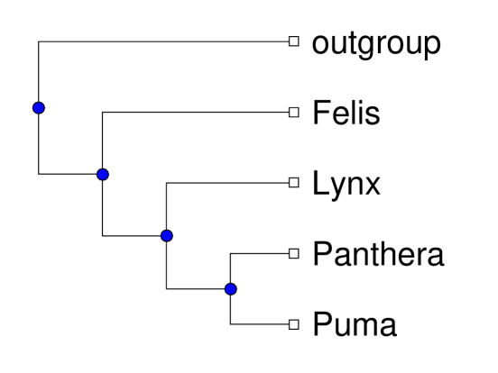
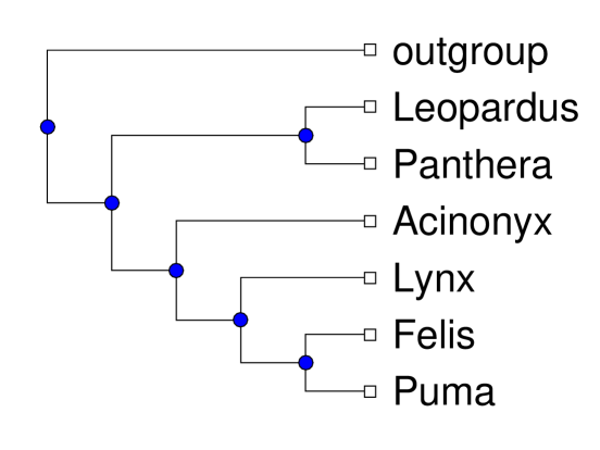
Figure 1: Phylogenetic trees from [Fulton and Strobeck (2006)] on the left and from [Flynn et al. (2005)] on the right, abstracted to genus-level (for more details, see Section 4).

The problem of combining a set of phylogenetic trees with (partially) overlapping sets of taxa into a single tree is known as the supertree construction problem. In the special case where each source tree contains exactly the same set of species, it is also called the consensus tree problem [Steel et al. (2000)]. In order to combine trees with different taxa, one needs a way to split the source trees into smaller structures which describe the relationships in the trees at the same time. There are several ways to achieve this, for instance by using triplets (rooted substructures with three leaf nodes) or quartets (unrooted substructures with four leaf nodes).

A quartet (topology) is an unrooted topological substructure of a tree. The quartet $((I,J),\allowbreak(K,L))$ is in its canonical representation if $I\mathchar 60\relax J$, $I\mathchar 60\relax K$, and $K\mathchar 60\relax L$, where “$\mathchar 60\relax$” refers to the alphabetical ordering of the names of the taxa. From now on, we will consider canonical representations of quartets. We say that a tree $T$ displays a quartet $((I,J),\allowbreak(K,L))$, if there is an edge in the tree $T$ that separates $T$ into two subtrees so that one subtree contains the pair $I$ and $J$ as its leaves and the other subtree contains the pair $K$ and $L$ as its leaves. For any set of four taxa appearing in a resolved phylogenetic tree $T$, there is exactly one quartet displayed by $T$. Furthermore, we say that two phylogenetic trees $T$ and $T^{\prime}$ are not compatible, if there is a set of four taxa for which $T$ and $T^{\prime}$ display a different quartet.

Example 1

Consider the two phylogenetic trees in Figure 1. It is easy to see that these trees are not compatible. For the taxa Felis, Lynx, Panthera, and Puma, the tree on the left displays the quartet ((Felis,Lynx),(Panthera,Puma)), while the tree on the right displays the quartet ((Felis,Puma),(Lynx,Panthera)).   $\blacksquare$

Let $\mathrm{tx}(T)$ denote the set of taxa in the leaves of a tree $T$ and $\mathrm{qt}(T)$ the set of all quartets that are displayed by $T$. For a collection $S$ of phylogenetic trees, we define $\mathrm{qt}(S)$ as the multiset $\bigcup_{T\in S}\mathrm{qt}(T)$ and $\mathrm{tx}(S)\mathchar 61\relax\bigcup_{T\in S}\mathrm{tx}(T)$. Given any phylogenetic tree $T$, the set $\mathrm{qt}(T)$ uniquely determines it [Erdős et al. (1999)].

The quartet compatibility problem is about finding out whether a set of quartet topologies $\mathrm{qt}(S)$ for a collection of phylogenetic trees $S$ is compatible, i.e., if there is a phylogeny $T$ on the taxa in $\mathrm{tx}(S)$ that displays all the quartet topologies in $\mathrm{qt}(S)$. The maximum quartet consistency problem for a supertree takes as input a set of quartet topologies $\mathrm{qt}(S)$ for a collection of phylogenetic trees $S$, and the goal is to find a phylogeny $T$ on the taxa $\mathrm{tx}(S)$ that displays the maximum number of quartet topologies in $\mathrm{qt}(S)$ [Piaggio-Talice et al. (2004)].

The topology of a tree $T$ can be captured more directly using projections of $T$. Given a set $S\subseteq\mathrm{tx}(T)$, the projection of $T$ with respect to $S$, denoted by $T_{S}$, is obtained from $T$ by removing all structure related to the taxa in $\mathrm{tx}(T)\setminus S$. This may imply that entire subtrees are removed and non-branching nodes are deleted. We say that $T$ displays another tree $T^{\prime}$ if $\mathrm{tx}(T^{\prime})\subseteq\mathrm{tx}(T)$ and $T_{\mathrm{tx}(T^{\prime})}\mathchar 61\relax T^{\prime}$.

Example 2

If the left tree in Figure 1 is projected with respect to $\{\emph{Puma},\emph{Lynx},\emph{Felis}\}$, the following tree results: ((Puma,Lynx),Felis). The right tree yields a different projection ((Puma,Felis),Lynx) illustrating the topological difference of the trees.   $\blacksquare$

When comparing a phylogeny $T$ with other phylogenies, an obvious question is which projections should be used. Rather than using arbitrary sets $S\subseteq\mathrm{tx}(T)$ for projections $T_{S}$, we suggest to use the subtrees of $T$. We denote this set by $\mathrm{sub}(T)$. It is clear that $T$ displays $T^{\prime}$ for every $T^{\prime}\in\mathrm{sub}(T)$. Moreover, if $T$ displays $T^{\prime\prime}$ for every $T^{\prime\prime}\in\mathrm{sub}(T^{\prime})$ and $\mathrm{tx}(T)\mathchar 61\relax\mathrm{tx}(T^{\prime})$, then $T\mathchar 61\relax T^{\prime}$. More generally, the more subtrees of $T^{\prime}$ are displayed by $T$, the more alike $T$ and $T^{\prime}$ are as trees. This observation suggests defining the maximum projection consistency problem for a supertree in analogy to the maximum quartet consistency problem. The input for this problem consists of the multiset $\mathrm{sub}(T_{1})\;\cup\;\ldots\;\cup\;\mathrm{sub}(T_{n})$ induced by a given collection $T_{1},\ldots,T_{n}$ of phylogenetic trees. The goal is to find a supertree $T$ such that $\mathrm{tx}(T)\mathchar 61\relax\mathrm{tx}(\{T_{1},\ldots,T_{n}\})$ and $T$ displays as many subtrees from the input as possible—disregarding orientation. This objective is aligned with the quartet-based approach: if $T$ displays a particular subtree $T^{\prime}$, then it also displays $\mathrm{qt}(T^{\prime})$.

Example 3

Consider again the trees in Figure 1. The non-trivial subtrees of the left tree are:

(outgroup,(Felis,(Lynx,(Panthera,Puma)))), (Felis,(Lynx,(Panthera,Puma))), (Lynx,(Panthera,Puma)), (Panthera,Puma)

The right tree displays only the subtree (Panthera,Puma) as its projection.   $\blacksquare$

3 Encodings for supertree optimization

We assume that the reader is familiar with basic ASP terminology and definitions, and we refer the reader to [Baral (2003), Gebser et al. (2012)] for details. Our encodings are based on the input language of the gringo 3.0.4 grounder [Gebser et al. (2009)] used to instantiate logic programs. In this section, two alternative encodings for the supertree construction problem are presented. Both encodings rely on the same formalization of the underlying tree structure, but have different objective functions as well as different representations for the input data. We begin by developing a canonical representation for phylogenies based on ordered trees in Section 3.1. The first encoding based on quartet information is then presented in Section 3.2. The second one exploiting projections of trees is developed in Section 3.3.

3.1 Canonical phylogenies

Our encodings formalize phylogenies as ordered trees whose leaf nodes correspond to taxa (species or genera) of interest. The simplest possible (atomic) tree consists of a single node. Thus we call the leaves of the tree atoms and formalize them in terms of the predicate and atom/1. We assume that the number of atoms is available through the predicate and atomcnt/1, and furthermore that atoms have been ordered alphabetically so that the first atom is accessible through the predicate and fstatom/1, while the predicate and nxtatom/2 provides the successor of an atom. These predicates can be straightforwardly expressed in the input language of gringo and we skip their actual definitions. Full encodings are published with tools (see Section 4).

To formalize the structure of an ordered tree with $N$ leaves, we index the leaf nodes using numbers from 1 to $N$. Any subsequent numbers up to $2N\mathchar 45\relax 1$ will be assigned to inner nodes as formalized by lines 2–4 of Listing 1. Depending on the topology of the tree, the number of inner nodes can vary from $1$ to $N\mathchar 45\relax 1$. In the former case, the tree has an edge from the root to every leaf but a full binary tree results in the latter case. If viewed as phylogenies, the former leaves all relationships unresolved whereas the latter gives a fully resolved phylogeny.

Listing 1: An ASP Encoding of Directed Trees/Forests

⬇

1% Domains

2node(1..2*N-1) :- atomcnt(N).

3leaf(X) :- node(X), X<=N, atomcnt(N).

4inner(X) :- node(X), X>N, atomcnt(N).

5pair(X,Y) :- inner(X), node(Y), X>Y.

6

7% Choose edges

8{ edge(X,Y): pair(X,Y) } 2*N-2 :- atomcnt(N).

9:- edge(X,Z), edge(Y,Z), pair(X;Y,Z), X<Y.

10:- edge(X,Y), pair(X,Y), inner(Y), not edge(Y,Z): pair(Y,Z).

11

12% Assign atoms to leaves

13asgn(1,A) :- node(1), fstatom(A).

14asgn(N+1,B) :- node(N), asgn(N,A), nxtatom(A,B).

The predicate and pair/2 defined in line 5 declares that the potential edges of the tree always proceed in the descending order of node numbers. This scheme makes loops impossible and prohibits edges starting from leaf nodes. The rule in line 8 chooses at most $2N\mathchar 45\relax 2$ edges for the tree up to $2N\mathchar 45\relax 1$ nodes. The constraint in line 9 ensures that a directed tree/forest rather than a directed acyclic graph is obtained. The purpose of the constraint in line 10 is to deny branches ending at inner nodes. The fixed assignment of atoms to leaf nodes $1\ldots N$ according to their alphabetical order takes place in lines 13–14 using predicates and fstatom/1 and and nxtatom/2. This is justified by a symmetry reduction, since $N!$ different assignments to leaf nodes would be considered otherwise and no tree topology is essentially ruled out.

However, as regards tree topologies themselves, further symmetry reductions are desirable because the number of optimal phylogenies can increase substantially otherwise. Listing 2 provides conditions for a canonical ordering for the inner nodes. The and order/2 predicate defined in lines 2–3 captures pairs of inner nodes that must be topologically ordered in a tree being constructed. The and ireach/2 predicate defined by rules in lines 4 and 5 gives the irreflexive reachability relation for nodes, i.e., a node is not considered reachable from itself. The constraint in line 6 effectively states that the numbering of inner nodes must follow the depth-first descending order, i.e., any inner nodes and X below and Y must have higher numbers than and Z. The remaining degree of freedom concerns the placement of leaves to subtrees. To address this, we need to find out the minimum leaf (node) for each subtree. The and min/2 predicate defined in lines 9–10 captures the actual minimum leaf and Y beneath an inner node and X. The orientation constraint in line 11 concerns inner nodes and Y and and Z subject to topological ordering, identifies the minimum leaf and W in the subtree rooted at and Z, and ensures that this leaf is smaller than any leaf and V in the subtree rooted at  and Y. This also covers the case that and V is the respective minimum leaf under and Y. The orientation constraint above generalizes that of [Brooks et al. (2007)] for non-binary trees and we expect that canonical trees will have further applications beyond this work.

Listing 2: Encoding for Canonical Phylogenies

⬇

1% Depth-first ordering on internal nodes

2order(Y,Z) :- edge(X,Y), edge(X,Z), pair(X,Y;Z), inner(Y;Z),

3 Y>Z, not edge(X,W): Y>W: W>Z: pair(X,W).

4ireach(X,Y) :- edge(X,Y), pair(X,Y).

5ireach(X,Y) :- ireach(X,Z), edge(Z,Y), pair(Z,Y).

6:- order(Y,Z), pair(Y,Z), ireach(Y,X), inner(X), X<Y.

7

8% Determine the orientation of leaf nodes

9min(X,Y) :- ireach(X,Y), inner(X), leaf(Y),

10 not ireach(X,Z): Z<Y: leaf(Z).

11:- order(Y,Z), pair(Y,Z), ireach(Y,V), min(Z,W), leaf(V;W), V<W.

12

13% Constraints for phylogenies

14:- unused(X), used(Y), inner(X;Y), X<Y.

15:- root(X), root(Y), inner(X;Y), X<Y.

16:- not root(X): inner(X).

17:- leaf(X), not edge(Y,X): pair(Y,X).

18:- inner(X), root(X), not outgroup(X).

19:- inner(X), not root(X), outgroup(X).

20:- edge(X,Y), pair(X,Y), not edge(X,Z): pair(X,Z): Z!=Y.

Finally, there are some further requirements specific to phylogenies. We assume that certain subsidiary predicates have already been defined. The predicate and root/1 is used to identify root nodes. Inner nodes that remain completely disconnected are marked as unused by the predicate and unused/1. Otherwise, the node is in use as captured by and used/1. Moreover, a node is an outgroup node, formalized by and outgroup/1, if it is assigned to the special outgroup taxon or one of its child nodes is so assigned (cf. Figure 1). Lines 14–20 list the additional constraints for a phylogeny. Only the highest numbers are allowed for unused nodes (line 14). The root must be a unique inner node (lines 15 and 16). Every leaf must be connected (line 17). The special outgroup leaf must be associated with the root node (lines 18 and 19). Every inner node that is actually used must have at least two children (line 20): the denial of unary nodes is justified because they are not meaningful for phylogenies.

3.2 Quartet-based approach

The first encoding is quartet-based. Each source tree is represented as the set of all quartets that it displays. The predicate and quartet/4 represents one input quartet in canonical form. Listing 3 shows the objective function for the quartet encoding. For each quartet appearing in the input, we check if it is satisfied by the current output tree candidate. The auxiliary predicate and reach/2 marks reachability from inner nodes to atoms (species) assigned to leaves. The output tree is rooted, so given any inner node and X in the tree, there is a uniquely defined subtree rooted at and X, and and reach(X,A) is true for any atom and A corresponding to a leaf node of the subtree. A quartet consisting of two pairs is satisfied by the output tree, if for one pair there exists at least one inner node and X such that the members of the pair are descendants of and X, while the members of the other pair do not appear in that subtree.

The predicate and quartetwt/5 assigns a weight to each quartet structure. In the unweighted case, this weight is equal to the number of source trees that display the quartet. In the weighted case, source trees stemming from computational studies based on molecular input data were weighted up by a factor of four. For example, if a particular quartet was present in three source trees, two of which were from molecular studies while the third one was not, the total weight would be $4\mathchar 43\relax 4\mathchar 43\relax 1$.

Listing 3: Optimization function for the quartet encoding

⬇

1reach(X,A) :- inner(X), ireach(X,Y), asgn(Y,A), atom(A).

2

3% Maximize number of satisfied quartets

4satisfied(A1,A2,A3,A4) :- quartet(A1,A2,A3,A4), inner(X),

5 reach(X,A1), reach(X,A2), not reach(X,A3), not reach(X,A4).

6satisfied(A1,A2,A3,A4) :- quartet(A1,A2,A3,A4), inner(X),

7 reach(X,A3), reach(X,A4), not reach(X,A1), not reach(X,A2).

8

9#maximize [ satisfied(A1,A2,A3,A4)=W: quartetwt(A1,A2,A3,A4,W) ].

3.3 Projection-based approach

The second encoding is based on direct projections of trees and the idea is to identify which inner nodes in the selected phylogeny correspond to subtrees present in the input trees. Input trees are represented using a function symbol and t as a tree constructor. For instance, the leftmost tree in Figure 1 is represented by a term

$$\and{t(outgroup,t(felis,t(lynx,t(panthera,puma))))}\mathbin{\cdot}$$ (1)

For simplicity, it is assumed here that and t always takes two arguments although in practice, some of the input trees are non-binary, and a more general list representation is used instead. In the encoding, projections of interest are declared in terms of the predicate and proj/1. The predicate and comp/1, defined in line 2 of Listing 4, identifies compound trees as those having at least one instance of the constructor and t. The set of projections is made downward closed by the rule in line 3. For instance, and outgroup and and t(felis,t(lynx,t(panthera,puma))) are projections derived from (1) by a single application of this rule. In line 4, atoms are recognized as trivial tree projections with no occurrences of and t such as and outgroup above.

Listing 4: Projection-Based Optimization of the Phylogeny

⬇

1% Projections of the phylogeny

2comp(t(T1,T2)) :- proj(t(T1,T2)).

3proj(T1;T2) :- comp(t(T1,T2)).

4atom(X) :- proj(X), not comp(X).

5

6% Reachability from a node to a projection

7reach(X,T) :- node(X), asgn(X,T), proj(T).

8reach(X,T) :- ireach(X,Y), node(X;Y), reach(Y,T), proj(T).

9

10% Assign compound trees to inner nodes

11asgn(X,T) :- inner(X), used(X), not denied(X,T), comp(T).

12denied(X,T) :- edge(X,Y), pair(X,Y), comp(T), reach(Y,T).

13denied(X,t(T1,T2)) :- edge(X,Y), pair(X,Y), comp(t(T1,T2)),

14 T1<T2, reach(Y,T1), reach(Y,T2).

15denied(X,t(T1,T2)) :- inner(X), used(X), comp(t(T1,T2)),

16 not reachvia(X,Z,T1): pair(X,Z).

17denied(X,t(T1,T2)) :- inner(X), used(X), comp(t(T1,T2)),

18 not reachvia(X,Z,T2): pair(X,Z).

19reachvia(X,Y,T) :- edge(X,Y), pair(X,Y), reach(Y,T), proj(T).

20:- inner(X), used(X), not asgn(X,T): comp(T).

21

22% Optimize the assignment of compound trees

23unassigned(T) :- comp(T), not asgn(X,T): node(X).

24next(X,T) :- edge(X,Y), pair(X,Y), asgn(Y,T), proj(T).

25separated(t(T1,T2)) :- edge(X,Y), pair(X,Y), asgn(X,t(T1,T2)),

26 not next(X,T1).

27separated(t(T1,T2)) :- edge(X,Y), pair(X,Y), asgn(X,t(T1,T2)),

28 not next(X,T2).

29#minimize [ unassigned(T)=AC*W: acnt(T,AC): projwt(T,W): comp(T),

30 separated(T)=W: projwt(T,W): comp(T) ].

The and reach/2 predicate, defined in lines 7 and 8 of Listing 4, generalizes the respective predicate from Listing 3 for arbitrary projections and T and includes a new base case for immediate assignments (line 7). A compound tree and T is assigned to an inner node and X by default (line 11) and the predicate and denied/2 is used to specify exceptions in this respect. It is important to note that if and edge(X,Y) is true, then and X is an inner node and and used(X) is true, too. The first exception (line 12) is that and T is already assigned below and X in the phylogeny. The second case (lines 13–14) avoids mapping distinct subtrees of and t(T1,T2) on the same subtree in the phylogeny. Thirdly, if and t(T1,T2) is to be assigned at inner node and X, then and T1 and and T2 must have been assigned beneath and X in the phylogeny (lines 15–18). Finally, the constraint in line 20 insists that each inner node is assigned at least one projection because the node could be removed from the phylogeny otherwise. The net effect of the constraints introduced so far is that if and T1 and and T2 have been assigned to nodes and X and and Y, respectively, then and t(T1,T2) is assigned to the least common ancestor of and X and and Y.

The rest of Listing 4 concerns the objective function we propose for phylogeny optimization. The predicate and unassigned/1 captures compound trees and T which could not be assigned to any inner node by the rules above. This is highly likely if mutually inconsistent projections are provided as input. It is also possible that a compound projection and t(T1,T2) is assigned further away from the subtrees and T1 and and T2, i.e., they are not placed next to and t(T1,T2). The predicate and separated/1 holds for and t(T1,T2) in this case (lines 24–28). The purpose of the objective function (line 30) is to minimize penalties resulting from these aspects of assignments. For unassigned compound trees and T, this is calculated as the product of the number of atoms in and T and the weight of and T. These numbers are accessible via auxiliary predicates and acnt/2 and and projwt/2 in the encoding. Separated compound trees are further penalized by their weight (line 29). Since the rules in lines 2–3, 13–18, 25–28 only cover binary trees they would have to be generalized for any fixed arity which is not feasible. To avoid repeating the rules for different arities, we represent trees as lists (of lists) in practice.

4 Experiments

Data.

We use a collection of 38 phylogenetic trees from [Säilä et al. (2011), Säilä et al. (2012)] covering 105 species of Felidae as our source trees. There are both resolved and unresolved trees, all rooted with outgroup, in the collection and the number of species varies from 4 to 52. The total number of species in the source trees makes supertree analysis even with heuristic methods challenging, and computing the full supertree for all species at once is not feasible with our encodings. Thus, we consider the following simplifications of the data. In Section 4.1 we use genus-specific projections of source trees to compare the efficiency of our two encodings. In Section 4.2 we reduce the size of the instance by considering the genus-level supertree as a first step towards solving the supertree problem for the Felidae data.

Experimental setting.

We used two identical 2.7-GHz CPUs with 256 GB of RAM to compute optimal answer sets for programs grounded by gringo 3.0.4. The state-of-the-art solver clasp 3.1.2 [Gebser et al. (2011)] was compared with a runner-up solver wasp [Alviano et al. (2015)] as of 2015-06-28. Moreover, we studied the performance of MAXSAT solvers as back-ends using translators lp2acyc 1.29 and lp2sat 1.25 [Gebser et al. (2014)], and a normalizer lp2normal 2.18 [Bomanson et al. (2014)] from the asptools collection. As MAXSAT solvers, we tried clasp 3.1.2 in its MAXSAT mode (clasp-s in Table 1), an openwbo-based extension [Martins et al. (2014)] of acycglucose R739 (labeled acyc in Table 1) also available in the asptools collection, and sat4j [Le Berre and Parrain (2010)] dated 2013-05-25.

4.1 Genus-specific supertrees

To produce genus-specific source trees for a genus $G$, we project all source trees to the species in $G$ (and the outgroup). Genera with fewer than five species are excluded as too trivial. Thus, the instances of Felidae data have between 6 and 11 species each, and the number of source trees varies between 2 and 22. In order to be able to compare the performance of different solvers for our encodings, we compute one optimum here and use a timeout of one hour. In Table 1 we report the run times for the best-performing configuration of each solver for both encodings. Moreover, the methods based on unsatisfiable cores turned out to be ineffective in general. Hence, branch-and-bound style heuristics were used.

The performance of the projection encoding scales up better than that of the quartet encoding when the complexity of the instance grows. Our understanding is that in the quartet encoding the search space is more symmetric than in the projection encoding: in principle any subset of the quartets could do and this has to be excluded in the optimality proof. On the other hand, the mutual incompatibilities of projections can help the solver to cut down the search space more effectively.

			clasp		wasp		acyc		clasp-s
Genus	Taxa	Trees	qtet	proj	qtet	proj	qtet	proj	qtet	proj
Hyperailurictis	6	2	0.0	0.0	0.0	0.0	0.0	0.0	0.0	0.0
Lynx	7	8	0.0	0.0	0.0	0.1	0.0	0.0	0.0	0.0
Leopardus	8	6	0.6	0.1	1.7	0.2	1.1	0.4	0.6	0.1
Dinofelis	9	2	0.1	0.0	0.0	0.1	0.1	0.1	0.0	0.1
Homotherium	9	3	0.7	0.0	0.1	0.1	0.1	0.0	0.0	0.0
Felis	11	12	39.6	21.9	290.8	120.6	122.7	59.6	27.7	20.8
Panthera	11	22	1395.8	45.6	–	456.3	–	174.6	944.2	67.1

Table 1: Time (s) to find one optimum for genus-specific data using different solvers using quartet (qtet) and projection (proj) encoding (– marks timeout).

4.2 Genus-level abstraction

We generate 28 trees abstracted to the genus level from the 38 species-level trees. The abstraction is done by placing each genus $G$ under the node $N$ furthest away from the root such that all occurrences of the species of genus $G$ are in the subtree below $N$. Finally, redundant (unary) inner nodes are removed from the trees. The trees that included fewer than four genera were excluded. Following [Säilä et al. (2011), Säilä et al. (2012)], Puma pardoides was treated as its own genus Pardoides, and Dinobastis was excluded as an invalid taxon. As further preprocessing, we removed the occurrences of genera Pristifelis, Miomachairodus, and Pratifelis appearing in only one source tree each. These so-called rogue taxa have unstable placements in the supertree, due to little information about their placements in relation to the rest of the taxa. The rogue taxa can be a posteriori placed in the supertree in the position implied by their single source tree. After all the preprocessing steps, our genus-level source trees have 34 genera in total and the size of the trees varies from 4 to 22 genera.

We consider the following schemes from [Säilä et al. (2011), Säilä et al. (2012)]:

All-FM-bb-wgt

Analysis with a constraint tree separating the representatives of Felinae and Machairodontinae into subfamilies, with weight 4 given to source trees from molecular studies.

F-Mol

Analysis using molecular studies only and extinct species pruned out (leaving 20 source trees and 15 genera, which are all representatives of Felinae).

Noticeably, the first setting allows us to split the search space and to compute the supertree for Felinae and Machairodontinae separately. The best resolved tree in [Säilä et al. (2011), Säilä et al. (2012)] was obtained using the MRP supertree for F-Mol abstracted to the genus level as a constraint tree (scheme All-F-Mol-bb-wgt). We include the best resolved tree by [Säilä et al. (2011)] to the comparison as well.

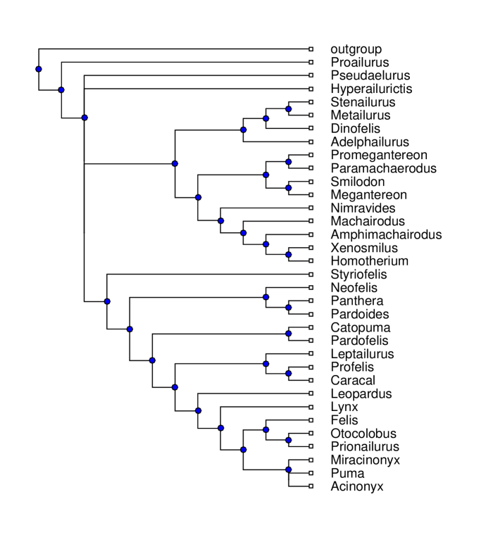
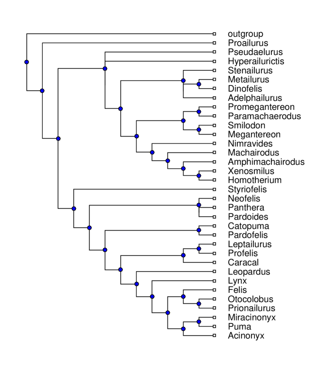
Figure 2: Left: Best-resolution 50% majority consensus MRP genus-level supertree modified from [Säilä et al. (2011), Säilä et al. (2012)] using scheme All-F-Mol-bb-wgt; Right: The optimal genus-level supertree using projection encoding and scheme All-FM-bb-wgt.

We use clasp for the computation of all optimal models. The considered schemes turned out to be unfeasible for the quartet-based encoding (no optimum was reached by a timeout of 48 hours), and only results from the projection encoding are included. It turns out that there exists a unique optimum for the projection encoding for both schemes. In the All-FM-bb-wgt scheme, the global optimum was identified in 4 hours and 56 minutes, while it was located in 52 minutes for F-Mol using --config=trendy which performed best on these instances. The respective run times are 1.5 hours and 20 minutes using parallel clasp 3.1.2 with 16 threads.

The MRP supertrees in [Säilä et al. (2011), Säilä et al. (2012)] are computed using the full species-level data with the Parsimony Ratchet method [Nixon (1999)]. For the resulting shortest trees, 50% majority consensus trees were computed and the best supported supertree according to [Wilkinson et al. (2005)] out of different runs (with various MRP settings) originates from scheme All-FM-bb-wgt, while the best resolved tree was obtained using scheme All-F-Mol-bb-wgt. Finally, the species-level supertree is collapsed to the genus level. The optimal supertree for the projection encoding and the MRP supertrees from [Säilä et al. (2011)] described above (projected to the set of genera considered in our experiments) are presented in Figure 2 and the online appendix (Appendices A–C).

As the true supertree is not known for this real-life dataset, the goodness of the output tree can only be measured based on how it reflects the source trees. To assess the quality of the output trees and to compare them with the MRP trees, we considered the number of satisfied quartets of source trees, the resolution of the supertree, and support values [Wilkinson et al. (2005)]. Support varies between $1$ and $\mathchar 45\relax 1$, indicating good and poor support, respectively, of the relationships in source trees. The results are given in Table 2, showing that the optimum of the projection encoding satisfies more quartets of the input data than the MRP supertrees.

Scheme	Method	Resolution	QS	%QS	V
All-FM-bb-wgt	proj	0.90	14 076	0.84	0.43
All-FM-bb-wgt	MRP	0.85	12 979	0.77	0.45
All-F-Mol-bb-wgt	MRP	0.93	13 910	0.83	0.42
F-Mol	proj	1.00	4 395	0.86	0.25
F-Mol	MRP	1.00	4 389	0.86	0.27

Table 2: Comparison between the optimal supertree for the projection encoding (proj) and the best MRP supertrees.

Finally, the differences of the objective functions of our two encodings can be illustrated by computing the supertree of 5 highly conflicting source trees of 8 species of hammerhead sharks from [Cavalcanti (2007)]. The optimum for the projection encoding is exactly the same as source tree (b) in [Cavalcanti (2007)], whereas the optimum for quartet encoding is exactly the same as source tree (a). Thus, the two objective functions are not equivalent in the case of conflicting source trees.

5 Conclusion

In this paper we propose two ASP encodings for phylogenetic supertree optimization. The first, solving the maximum quartet consistency problem, is similar to the encoding in [Wu et al. (2007)] and does not perform too well in terms of run time when the size of the input (source trees and number of taxa therein) grows. The other novel encoding is based on projections of trees and the respective optimization problem is formalized as the maximum projection consistency problem. We use real data, namely a collection of phylogenetic trees for the family of cats (Felidae) and first evaluate the performance of our encodings by computing genus-specific supertrees. We then compute a genus-level supertree for the data and compare our supertree against a recent supertree computed using MRP approach [Säilä et al. (2011), Säilä et al. (2012)]. The projection-based encoding performs better than the quartet-based one and produces a unique optimum for the two cases we consider (with rogue taxa removed). Obviously, this is not the case in general and in the case of several optima, consensus and majority consensus supertrees can be computed. Furthermore, our approach produces supertrees comparable to ones obtained using MRP method. For the current projection-based encoding, the problem of optimizing a species-level supertree using the Felidae data is not feasible as a single batch. Further investigations how to tackle the larger species-level data are needed. Possible directions are for instance using an incremental approach and/or parallel search.

6 Acknowledgments

This work has been funded by the Academy of Finland, grants 251170 (Finnish Centre of Excellence in Computational Inference Research COIN), 132995 (LS), 275551 (LS), and 250518 (EO). We thank Martin Gebser, Ian Corfe, and anonymous reviewers for discussion and comments that helped to improve the paper.

References

- Aho et al. (1981) Aho, A. V., Sagiv, Y., Szymanski, T. G., and Ullman, J. D. 1981. Inferring a tree from lowest common ancestors with an application to the optimization of relational expressions. SIAM Journal on Computing 10, 3, 405–421.
- Alviano et al. (2015) Alviano, M., Dodaro, C., Leone, N., and Ricca, F. 2015. Advances in WASP. In Proceedings of the 13th International Conference on Logic Programming and Nonmonotonic Reasoning, LPNMR 2015. Lecture Notes in Computer Science, vol. 9345. Springer.
- Baral (2003) Baral, C. 2003. Knowledge Representation, Reasoning, and Declarative Problem Solving. Cambridge University Press, New York, NY, USA.
- Baum (1992) Baum, B. R. 1992. Combining trees as a way of combining data sets for phylogenetic inference, and the desirability of combining gene trees. Taxon 41, 1, 3–10.
- Bininda-Emonds (2004) Bininda-Emonds, O. R. 2004. Phylogenetic Supertrees: Combining Information to Reveal the Tree of Life. Computational Biology. Springer.
- Bomanson et al. (2014) Bomanson, J., Gebser, M., and Janhunen, T. 2014. Improving the normalization of weight rules in answer set programs. In Proceedings of the 14th European Conference on Logics in Artificial Intelligence, JELIA 2014. Lecture Notes in Computer Science, vol. 8761. Springer, 166–180.
- Brooks et al. (2007) Brooks, D. R., Erdem, E., Erdoğan, S. T., Minett, J. W., and Ringe, D. 2007. Inferring phylogenetic trees using answer set programming. Journal of Automated Reasoning 39, 4, 471–511.
- Bryant (1997) Bryant, D. 1997. Building trees, hunting for trees, and comparing trees. Ph.D. thesis, University of Canterbury.
- Byrka et al. (2010) Byrka, J., Guillemot, S., and Jansson, J. 2010. New results on optimizing rooted triplets consistency. Discrete Applied Mathematics 158, 11, 1136–1147.
- Cavalcanti (2007) Cavalcanti, M. J. 2007. A phylogenetic supertree of the hammerhead sharks (Carcharhiniformes, Sphyrnidae). Zoological Studies 46, 1, 6–11.
- Chen et al. (2003) Chen, D., Diao, L., Eulenstein, O., Fernández-Baca, D., and Sanderson, M. 2003. Flipping: a supertree construction method. DIMACS series in discrete mathematics and theoretical computer science 61, 135–162.
- Chimani et al. (2010) Chimani, M., Rahmann, S., and Böcker, S. 2010. Exact ILP solutions for phylogenetic minimum flip problems. In Proceedings of the First ACM International Conference on Bioinformatics and Computational Biology, BCB 2010. ACM, 147–153.
- Day et al. (1986) Day, W. H., Johnson, D. S., and Sankoff, D. 1986. The computational complexity of inferring rooted phylogenies by parsimony. Mathematical biosciences 81, 1, 33–42.
- Erdős et al. (1999) Erdős, P. L., Steel, M. A., Székely, L. A., and Warnow, T. 1999. A few logs suffice to build (almost) all trees (i). Random Structures and Algorithms 14, 2, 153–184.
- Flynn et al. (2005) Flynn, J. J., Finarelli, J. A., Zehr, S., Hsu, J., and Nedbal, M. A. 2005. Molecular phylogeny of the Carnivora (Mammalia): assessing the impact of increased sampling on resolving enigmatic relationships. Systematic Biology 54, 2, 317–337.
- Foulds and Graham (1982) Foulds, L. R. and Graham, R. L. 1982. The Steiner problem in phylogeny is NP-complete. Advances in Applied Mathematics 3, 1, 43–49.
- Fulton and Strobeck (2006) Fulton, T. L. and Strobeck, C. 2006. Molecular phylogeny of the Arctoidea (Carnivora): effect of missing data on supertree and supermatrix analyses of multiple gene data sets. Molecular phylogenetics and evolution 41, 1, 165–181.
- Gebser et al. (2014) Gebser, M., Janhunen, T., and Rintanen, J. 2014. Answer set programming as SAT modulo acyclicity. In Proceedings of the 21st European Conference on Artificial Intelligence, ECAI 2014. IOS Press, 351–356.
- Gebser et al. (2012) Gebser, M., Kaminski, R., Kaufmann, B., and Schaub, T. 2012. Answer Set Solving in Practice. Synthesis Lectures on Artificial Intelligence and Machine Learning. Morgan & Claypool Publishers.
- Gebser et al. (2009) Gebser, M., Kaminski, R., Ostrowski, M., Schaub, T., and Thiele, S. 2009. On the input language of ASP grounder Gringo. In Proceedings of the 10th International Conference on Logic Programming and Nonmonotonic Reasoning, LPNMR 2009. Lecture Notes in Computer Science, vol. 5753. Springer, 502–508.
- Gebser et al. (2011) Gebser, M., Kaufmann, B., Kaminski, R., Ostrowski, M., Schaub, T., and Schneider, M. T. 2011. Potassco: The Potsdam answer set solving collection. AI Commun. 24, 2, 107–124.
- Gent et al. (2003) Gent, I. P., Prosser, P., Smith, B. M., and Wei, W. 2003. Supertree construction with constraint programming. In Proceedings of the 9th International Conference on Principles and Practice of Constraint Programming, CP 2003. Lecture Notes in Computer Science, vol. 2833. Springer, 837–841.
- Goloboff and Pol (2002) Goloboff, P. A. and Pol, D. 2002. Semi-strict supertrees. Cladistics 18, 5, 514–525.
- Kavanagh et al. (2006) Kavanagh, J., Mitchell, D. G., Ternovska, E., Manuch, J., Zhao, X., and Gupta, A. 2006. Constructing Camin-Sokal phylogenies via answer set programming. In Proceedings of the 13th International Conference on Logic for Programming, Artificial Intelligence, and Reasoning, LPAR 2006. Lecture Notes in Computer Science, vol. 4246. Springer, 452–466.
- Le et al. (2012) Le, T., Nguyen, H., Pontelli, E., and Son, T. C. 2012. ASP at work: An ASP implementation of PhyloWS. In Technical Communications of the 28th International Conference on Logic Programming, ICLP 2012. LIPIcs, vol. 17. 359–369.
- Le Berre and Parrain (2010) Le Berre, D. and Parrain, A. 2010. The Sat4j library, release 2.2. Journal on Satisfiability, Boolean Modeling and Computation 7, 59–64.
- Martins et al. (2014) Martins, R., Manquinho, V., and Lynce, I. 2014. Open-WBO: a modular MaxSAT solver. In Theory and Applications of Satisfiability Testing, SAT 2014. Lecture Notes in Computer Science, vol. 8561. Springer, 438–445.
- Morgado and Marques-Silva (2010) Morgado, A. and Marques-Silva, J. 2010. Combinatorial optimization solutions for the maximum quartet consistency problem. Fundam. Inform. 102, 3-4, 363–389.
- Nixon (1999) Nixon, K. C. 1999. The parsimony ratchet, a new method for rapid parsimony analysis. Cladistics 15, 4, 407–414.
- Piaggio-Talice et al. (2004) Piaggio-Talice, R., Burleigh, J. G., and Eulenstein, O. 2004. Quartet supertrees. In Phylogenetic Supertrees. Springer, 173–191.
- Purvis (1995) Purvis, A. 1995. A modification to Baum and Ragan’s method for combining phylogenetic trees. Systematic Biology 44, 2, 251–255.
- Ragan (1992) Ragan, M. A. 1992. Phylogenetic inference based on matrix representation of trees. Molecular phylogenetics and evolution 1, 1, 53–58.
- Säilä et al. (2012) Säilä, L. K., Fortelius, M., Oikarinen, E., Werdelin, L., and Corfe, I. 2012. Fossil mammals, phylogenies and climate: the effects of phylogenetic relatedness on range sizes and replacement patterns in changing environments. In Proceedings of 60th Annual Symposium of Vertebrate Palaeontology and Comparative anatomy, SVPCA 2012. Poster.
- Säilä et al. (2011) Säilä, L. K., Fortelius, M., Oikarinen, E., Werdelin, L., Corfe, I., and Tuomola, A. 2011. Taxon replacement: Invasion or speciation? First results for a supertree of Neogene mammals. Journal of Vertebrate Paleontology 31, 3, suppl., 184A.
- Semple and Steel (2000) Semple, C. and Steel, M. 2000. A supertree method for rooted trees. Discrete Applied Mathematics 105, 1, 147–158.
- Snir and Rao (2012) Snir, S. and Rao, S. 2012. Quartet MaxCut: a fast algorithm for amalgamating quartet trees. Molecular phylogenetics and evolution 62, 1, 1–8.
- Sridhar et al. (2008) Sridhar, S., Lam, F., Blelloch, G. E., Ravi, R., and Schwartz, R. 2008. Mixed integer linear programming for maximum-parsimony phylogeny inference. IEEE/ACM Transactions on Computational Biology and Bioinformatics 5, 3, 323–331.
- Steel et al. (2000) Steel, M., Dress, A. W., and Bocker, S. 2000. Simple but fundamental limitations on supertree and consensus tree methods. Systematic Biology 49, 2, 363–368.
- Swenson et al. (2011) Swenson, M. S., Suri, R., Linder, C. R., and Warnow, T. 2011. An experimental study of Quartets MaxCut and other supertree methods. Algorithms for Molecular Biology 6, 1, 7.
- Wilkinson et al. (2005) Wilkinson, M., Cotton, J. A., Creevey, C., Eulenstein, O., Harris, S. R., Lapointe, F.-J., Levasseur, C., Mcinerney, J. O., Pisani, D., and Thorley, J. L. 2005. The shape of supertrees to come: tree shape related properties of fourteen supertree methods. Systematic biology 54, 3, 419–431.
- Wilkinson et al. (2005) Wilkinson, M., Pisani, D., Cotton, J. A., and Corfe, I. 2005. Measuring support and finding unsupported relationships in supertrees. Systematic Biology 54, 5, 823–831.
- Wu et al. (2007) Wu, G., You, J.-H., and Lin, G. 2007. Quartet-based phylogeny reconstruction with answer set programming. IEEE/ACM Transactions on Computational Biology and Bioinformatics 4, 1, 139–152.