Pressure anisotropy and small spatial scales induced by velocity shear

Abstract

Non-Maxwellian metaequilibria can exist in low-collisionality plasmas as evidenced by satellite and laboratory measurements. By including the full pressure tensor dynamics in a fluid plasma model, we show that a sheared velocity field can provide an effective mechanism that makes an initial isotropic state anisotropic and agyrotropic. We discuss how the propagation of magneto-elastic waves can affect the pressure tensor anisotropization and its spatial filamentation which are due to the action of both the magnetic field and flow strain tensor. We support this analysis by a numerical integration of the nonlinear equations describing the pressure tensor evolution.

The aim of this Letter is to show that a sheared velocity field in a weakly collisional, magnetized plasma drives a macroscopic pressure anisotropization in the plane of the velocity strain tensor. This represents a general mechanism when collisional relaxation is absent or slow that causes part of the kinetic energy of the plasma flow to be locally transformed into anisotropic “internal energy”. This energy conversion implies that shear flows do not affect the plasma dynamics only through the fluid destabilization of Kelvin-Helmholtz (KH) modes KH or by breaking the correlation length of unstable modes Palermo ; Transp_barrier responsible e.g., for anomalous energy transport in magnetically confined plasmas, but can lead to the onset of additional phase space instabilities driven by the induced pressure anisotropy.

In magnetized plasmas the fast particle gyromotion in a sufficiently strong field makes the pressure tensor isotropic in the plane perpendicular to the magnetic field direction but allows for different parallel and perpendicular pressures (gyrotropic pressure as is the case for the double-adiabatic or CGLCGL closure). On the contrary, the fluid strain $\Sigma_{ij}\equiv\partial u_{i}/\partial x_{j}$ in the sheared fluid velocity ${u_{i}({\bm{x}})}$ has a twofold effect: first, through its rotational component it combines or competes with the gyrotropic effect due to the magnetic field, second it induces pressure anisotropy (agyrotropic pressure) in the plane perpendicular to the magnetic field (taken to coincide with the velocity shear plane) through its incompressible rate of shear (its symmetrical traceless component).

Here we discuss the role of the flow strain in the dynamic equations of the full pressure tensor as obtained from the second moment of Vlasov Equation (VE), thus going beyond both the CGL closure and the Finite Larmor Radius (FLR) correctionsCerri_1 approach. We focus in particular on the dynamics of the full pressure tensor within a 1-fluid description of a dissipationless magnetized plasma and show how the propagation of “magneto-elastic” waves can affect the pressure anisotropization and small spatial scale formation due to the interplay between the gyrotropic and the non-gyrotropic dynamics induced by the magnetic field and by the strain tensor.

Non-Maxwellian states, sometimes exhibiting pressure agyrotropyAstudillo ; Posner ; He , are observed both experimentallyMarsch ; CLUSTER ; Astudillo ; Posner ; He ; Tu ; Wind ; Aunai1 ; LEIA and in Vlasov simulationsServidio1 ; Galeotti ; also the role of a shear flow in affecting the kinetic properties of a collisionless or weakly collisional plasma is well established experimentally. Even if mechanisms based on the CGL paradigm are now almost acquired when explaining the main features of solar wind anisotropiesWind , the correlation between the presence of a velocity shear and the extent of anisotropy in particle distributions is evoked both for the core protons in the fast solar windTu and in “space simulation” laboratory experimentsLEIA . A sheared convection velocity in the Earth ionosphere is thought to play a role in the heating of ions and in the consequent plasma bulk upflow in the auroral regionAurorae . Moreover, the presence of a velocity shear is known to play an important role in the enhancement of a variety of pressure anisotropy-related plasma instabilities. The presence of a velocity shear in the near-Earth plasma sheet profile prior to a substorm expansion lowers the instability threshold of ion-Weibel modes in the geomagnetic tailYoon . The role of a vorticity-related velocity shear in generating a gyrotropic temperature anisotropy in ion temperature gradient (ITG) driven turbulence, was discussed in Ref.Transp_barrier in connection with the relaxation of transport barriers in tokamak plasmas. Finally, an anisotropic pressure tensor was shown to form during the nonlinear stage of the current-filamentation instability (CFI) arising in the presence of two opposite cold electron beams. This anisotropy was shown to increase the threshold and growth rate of the reconnection instability developing on the shoulder of the CFI-generated magnetic structuresCalifano1 . These also develop in the presence of radially inhomogeneous beams such as in high intensity laser-plasma interactionsCalifano2 and are measured in laboratory experimentsinertial .
In Ref.Kahn sufficient conditions for the instability of electromagnetic waves in an unmagnetized Vlasov plasma with a sheared velocity distribution were studied, showing that an anisotropic pressure tensor leads to the instability of transverse perturbations. This was applied in Albright to study the steady state achievable when the shear-induced temperature anisotropy balances the electron diffusion in the velocity space due to the growth of static magnetic perturbations generated by the pressure anisotropy itself. Anisotropic turbulence induced by a KH unstable velocity shearWerne and by a Von Karman flowMarie was also pointed out.

We start from the two-fluid equations of a collisionless magnetized plasma, obtained by evaluating the moments of VE. We neglect the electron dynamics (i.e. $m_{e}/m_{i}\rightarrow 0$) and temperature, whereas the components of the full pressure tensor contribute to ion dynamics. The $2^{nd}$ anisotropic ion moment, $\Pi_{ij}$, is closed by

$$\frac{\partial}{\partial t}\Pi_{ij}\,=\,-\underbrace{\mathcal{L}_{{\bf u}}(\Pi_{ij})}_{|\nabla{\bf u}|\equiv\tau_{H}^{-1}}\,+\,\underbrace{\mathcal{M}_{{\bf u}}(\Pi_{ij})}_{\Omega_{c}\equiv\tau_{B}^{-1}}$$ (1)

where $\Omega_{c}\equiv q|{\bm{B}}|/(mc)$ and we have introduced the linear operators $\mathcal{L}_{{\bf u}}(\Pi_{ij})\equiv{\partial_{k}}(u_{k}\Pi_{ij})+\Pi_{kj}{\partial_{k}}{u_{i}}+\Pi_{ik}\partial_{k}{u_{j}}$ and $\mathcal{M}_{{\bf u}}(\Pi_{ij})\equiv q/m\left(\varepsilon_{ilm}\Pi_{lj}B_{m}+\varepsilon_{jlm}\Pi_{il}B_{m}\right)$, and the corresponding characteristic hydrodynamic ($\tau_{{}_{H}}\equiv|\nabla{\bf u}|^{-1}$) and magnetic ($\tau_{{}_{B}}\equiv\Omega_{c}^{-1}$) time scales. The simplifying assumption, frequently used in the literature Hesse ; Khanna , of neglecting in Eq.(1) the divergence of the ion heat flux tensor, $Q_{ijk}\equiv\langle mn(v_{i}-u_{i})(v_{j}-u_{j})(v_{k}-u_{k})\rangle$, is consistent with the geometrical configuration considered later in this letter at least until very short spatial scales in the plane perpendicular to the magnetic field are formed during the nonlinear evolution. Typical closures of ${\bm{\Pi}}$ have been performed by means of a power expansion each in terms of some small parameter: including corrections in Eq.(1) due to a small collision time with respect to both $\tau_{{}_{H}}$ and $\tau_{{}_{B}}$, leads to Braginskii’s gyroviscous FLR modelBraginskii , while a small $\tau_{{}_{B}}/\tau_{{}_{H}}$ leads to FLR gyrotropic corrections to CGL equationsCerri_1 ; Khanna ; FLR_CGL . More recent FLR-Landau-fluid modelsFLR_LF also retain Landau-fluid effectsLandauFluid . Here we consider a dissipationless regime and do not assume the ratio $\tau_{{}_{B}}/\tau_{{}_{H}}$ to be small.
Defining the matrices ${\bf B}_{ij}\equiv\varepsilon_{ijm}B_{m}$, and ${\bf W}_{ij}\equiv$ $(\partial_{i}u_{j}-\partial_{j}u_{i})/2$ that describe the rotation induced by the magnetic field and by the shear flow respectively, the strain traceless matrix ${\bf D}_{ij}\equiv(\partial_{j}u_{i}+\partial_{i}u_{j})/2-C{\bm{\delta}}_{ij}$, the compression $C\equiv(\partial_{k}u_{k})/3$ and the derivative $d/dt\equiv\partial_{t}+u_{k}\partial_{k}$, Eq.(1) can be conveniently written as

$$\frac{d}{dt}{\bm{\Pi}}={[\mathcal{\bf B}+{\bf W},{\bm{\Pi}}]}-\{{\bf D},{\bm{\Pi}}\}-5C{\bm{\Pi}}$$ (2)

where $[\,,\,]$ denotes commutator and $\{\,,\,\}$ anticommutator. The first r.h.s. term shows that the magnetic field ${\bm{B}}$ and the flow vorticity ${\bm{\omega}}$ ($\omega_{i}\equiv\varepsilon_{ijk}W_{jk}$) combine to make ${\bm{\Pi}}$ to rotate around the axis of ${{\bf B}+{\bf W}}$. The perpendicular components rotate at twice the cyclotron frequency in absence of vorticity, or at twice the fluid rotation frequency in the unmagnetized case. If the axes of ${\bf B}$ and ${\bf W}$ are aligned the two frequencies add up if ${\bm{B}}\cdot{\bm{\omega}}>0$ and subtract if ${\bm{B}}\cdot{\bm{\omega}}<0$. The last r.h.s. term of Eqs.(2) acts isotropically on ${\bm{\Pi}}$ while the second term can induce pressure anisotropization whenever ${\bf D}$ is not zero.

First, we consider a model system with an incompressible shear flow $u^{0}_{y}(x)$ constant in time (energy is thus constantly injected from outside) in the presence of a uniform and constant magnetic field along the $z$-axis. In this model the velocity strain and the vorticity have the same magnitude, ${\bf B}$ is uniform in space, the axes of ${\bf B}$ and ${\bf W}$ are aligned along $z$ while ${\bf D}$ has no $z$ components. Eq.(2) leads to a linear system in which the components of ${\bm{\Pi}}$ perpendicular to ${\bm{B}}$ are decoupled from those having a parallel component and their determinant is constant. Three eigenvalues are obtained for the perpendicular components: $\gamma_{0}=0$, which corresponds to a stationary mode with $\Pi^{\gamma_{0}}_{yy}/\Pi^{\gamma_{0}}_{xx}=\Omega^{\prime}({x})/\Omega_{c}$ and $\Pi^{\gamma_{0}}_{xy}=0$, and $\gamma_{\pm}=\pm 2i\sqrt{\Omega_{c}\Omega^{\prime}(x)}$ with $\Pi^{\gamma_{\pm}}_{yy}/\Pi^{\gamma_{\pm}}_{xx}=-\Omega^{\prime}({x})/\Omega_{c}$ and $\Pi^{\gamma_{\pm}}_{xy}/\Pi_{xx}=\pm i\,\sqrt{\Omega^{\prime}({x})/\Omega_{c}}$. Here $\Omega^{\prime}({x})\equiv\Omega_{c}+\partial_{x}u_{y}^{0}(x)$. Provided $\Omega^{\prime}({x})>0$, the $\gamma_{0}$ mode can describe an equilibrium solution of Eq.(2) (in agreement with the self-consistent equilibria discussed in Cerri_2 ), $\Pi_{yy}/\Pi_{xx}=\Omega^{\prime}({x})/\Omega_{c}$ and $\Pi_{xy}=0$. The $\gamma_{\pm}$ modes represent either oscillations or growing and damped modes depending on the sign of $\Omega^{\prime}({\bm{x}})$. For $\Omega^{\prime}(x)>0$ the perpendicular pressure tensor components of an initial isotropic state with $\Pi_{xx}(x,0)=\Pi_{yy}(x,0)=P_{\perp}(x)$ oscillate in time around a mean value given by $\langle\Pi_{yy}(x,t)\rangle=(\Omega^{\prime}(x)/\Omega_{c})\langle\Pi_{xx}(x,t)\rangle=(\Omega^{\prime}(x)+\Omega_{c})P_{\perp}(x)/(2\Omega_{c})$ and $\langle\Pi_{xy}(x,t)\rangle=0$, the amplitude of the oscillations of $\Pi_{yy}(x,t)$ being $\partial_{x}u_{y}^{0}(x)P_{\perp}(x,0)/(2\Omega(x))$. In Fig.1 the profile of $\Pi_{yy}$ is shown at different times, for an initial pressure tensor $\Pi_{ij}=\delta_{ij}$, $B_{z}^{0}=1$ and $u_{y}^{0}=V_{0}{\cos}(kx)$ with $V_{0}=1.5$ and $k=1$. An important feature caused by the spatial inhomogeneity of the shear flow is the strongly inhomogeneous growth of the components of the pressure tensor, as regions where the evolution is oscillatory alternate, depending from the local sign of $\Omega^{\prime}\Omega$, with regions of exponential growth occurring over a time scale $\tau_{{}_{H}}=(kV_{0})^{-1}$. This gives rise to a spatially filamented pressure tensor.

Second, we consider the self-consistent (SC) case in which the flow and the e.m. fields evolve in time according to Eq.(1) and to the ideal MHD equations with an anisotropic ion pressure (note the Hall term in Ohm’s law to vanish identically for the examples discussed in this Letter). This system conserves the total energy ${E}^{tot}=\int d{\bm{x}}^{3}\left(\rho u^{2}/2+B^{2}/8\pi+\mbox{tr}\{{\bm{\Pi}}\}/2\right)$, and depends on three dimensionless parameters $\tau_{H}/\tau_{B}$ $=(c_{{}_{A}}/c_{{}_{H}})(L_{{}_{H}}/d_{i})$, $(c_{{}_{A}}/c_{{}_{H}})^{2}$ and $(c_{\perp}/c_{{}_{H}})^{2}$ with $L_{{}_{H}}$ the scalelength of the configuration, $c_{A}$ the Alfvèn velocity, $c_{{}_{H}}=L_{{}_{H}}/\tau_{{}_{H}}$ a measure of the flow velocity, $d_{i}\equiv c_{{}_{A}}/\Omega_{c}$ the ion skin depth, and $c_{\perp}\equiv P_{\perp}/\rho=c_{s}/\sqrt{2}$ with $c_{s}$ the “sound” velocity evaluated with respect to the initial ion pressure, assumed isotropic in the plane perpendicular to ${\bm{B}}$ comment_sound . Two parameters only, $(\tau_{{}_{H}}/\tau_{{}_{B}})/(c_{{}_{A}}/c_{{}_{H}})^{2}$ and $(\tau_{{}_{H}}/\tau_{{}_{B}})/(c_{\perp}/c_{{}_{H}})^{2}$, rule the linear dynamics. The CGL-FLR limit of Ref.Cerri_1 is recovered in the low frequency limit $\partial_{t}\ll\Omega_{c}$ for $(c_{{}_{H}}/c_{{}_{A}})(d_{i}/L_{{}_{H}})\ll 1$ and $d_{i}/L_{{}_{H}}\sim(c_{\perp}/c_{{}_{A}})d_{i}/L_{{}_{H}}\ll 1$, where no specific ordering for $c_{\perp}/c_{{}_{A}}$ is assumed.

In the SC case the anisotropization of the pressure tensor caused by the presence of an initially imposed shear flow is limited by the the reaction of the pressure tensor on the plasma flow which reduces its shear and by the excitation of nonlinear “magneto-elastic” perturbations that tend to propagate the shear of the velocity flow outwards. The main features of these pressure tensor and velocity perturbations can be understood by referring to the linear waves described by the SC system that propagate in a uniform, homogeneous equilibrium with ${\bm{B}}=B_{0}{\bm{e}}_{z}$, density $\rho_{0}$, double adiabatic pressure $\Pi_{ij}=P_{\perp}\delta_{ij}+(P_{||}-P_{\perp})B_{i}B_{j}/B^{2}$, and wave-vector ${\bf k}=k{\bm{e}}_{x}$. The resulting dispersion relation

$${(\omega^{2}-4\Omega^{2}-k^{2}c_{\perp}^{2})[\omega^{2}-k^{2}(c_{{}_{A}}^{2}+3c_{\perp}^{2})]}\displaystyle{-4\Omega^{2}k^{2}c_{\perp}^{2}=0},\\ \\$$ (3)

has a higher frequency branch HFB, $\omega^{2}_{h}\sim 4\Omega^{2}{+2k^{2}c_{\perp}^{2}}$ and $\omega^{2}_{h}\sim{k^{2}(c_{{}_{A}}^{2}+3c_{\perp}^{2})}$ for $k^{2}\to 0$, and $k^{2}\to\infty$ respectively, and a lower frequency branch LHB, $\omega^{2}_{l}\sim{k^{2}(c_{{}_{A}}^{2}+2c_{\perp}^{2})}$ and $\omega^{2}_{l}\sim{k^{2}c_{\perp}^{2}}$ for $k^{2}\to 0$, and $k^{2}\to\infty$. The $k^{2}\to 0$ limit of the LFB corresponds to the CGL form of a perpendicular magnetosonic wave. In the limit of vanishing magnetic field the two branches are not dispersive and reduce to a longitudinal and to a transverse sound mode propagating at phase velocities $\sqrt{3}c_{\perp}$ and $c_{\perp}$ respectively. Note that in this latter limit the SC system admits the propagation of finite-amplitude transverse waves where $u_{y}$ and $\Pi_{yy}$ satisfy the wave equation $\partial_{t}^{2}=c_{\perp}^{2}\partial_{x}^{2}$ and the energy continuity equation $\partial_{t}(\rho_{0}u_{y}^{2}+\Pi_{yy})=-\partial_{x}(u_{y}\Pi_{yy})$. When excited, these waves may carry away and disperse an initially imposed shear flow $u_{y}(x)$ with spatial scale $L_{{}_{H}}$ on time scales of the order of $L_{{}_{H}}/c_{{}_{A}}\sim L_{{}_{H}}/c_{\perp}$, thus reducing the anisotropization and the spatial inhomogeneity of the pressure tensor forced by the flow. This propagation might affect the onset of the KH instabilities in a collisionless weakly magnetized plasma. In the presence of a strong magnetic field these waves, in particular the HFB, couple the $x$ and the $y$ components of the plasma velocity. In addition they become dispersive with the group velocity of the HFB going to zero for $k\to 0$.

The nonlinear SC case has been integrated numerically starting from an isotropic initial condition with homogeneous density, ${\bm{B}}=B_{0}{\bm{e}}_{z}$ and ${\bm{u}}=u_{y}^{0}(x){\bf e}_{y}$, varying the value of the ratios of the three dimensionless parameters. In Figs.2-3 we consider the case with $u_{y}^{0}(x)=V_{0}\tanh(x/d_{i})/\cosh^{2}(x/d_{i})$ and $\tau_{{}_{H}}/\tau_{{}_{B}}=c_{{}_{A}}/c_{{}_{H}}=c_{\perp}/c_{{}_{H}}=1$. The results obtained can be qualitatively accounted for by referring to the linear modes described above where the initial shear velocity $u_{y}(x)$ is interpreted as an initial perturbation. Note that, though its characteristic scale-length is chosen of the order $d_{i}$, the initial Fourier spectrum peaks around $kd_{i}\lesssim 1$ (Fig.2).
The initial perturbation can be written as a superposition of the LFB and of the HFB. To leading order in $kd_{i}\ll 1$ the polarization vectors components in the $(u_{x},u_{y})$ basis are $(1,-i~{}o(kd_{i}))$ and $(1,-i)$ for $\omega_{l}$ and for $\omega_{h}$ respectively. This implies that the chosen initial perturbation corresponds to a superposition of the two branches with equal and opposite amplitudes and that the time evolution of $u_{y}(x)$ is mainly determined by that of the HFB. This is consistent with the results of the numerical integration and explains why the pressure agyrotropy (Figs.3), that in our geometry is mainly related to the spatial inhomogeneity of $u_{y}^{0}(x)$, tends to remain at the original position and not to be carried away at the Alfvènic group velocity of the LFB, at least until small spatial scales are formed which are instead transported away efficiently by the HFB. For example, at $x=0$ Figs.(3) show local peak agyrotropies $|\Pi_{yy}-\Pi_{xx}|/|\Pi_{yy}^{0}+\Pi_{xx}^{0}|$ of $0.12$, $0.22$ and $0.14$, and “mean anisotropies” $2\Pi_{zz}/(\Pi_{yy}+\Pi_{xx})$ of $1.02$, $2.35$ and $0.98$ for the $\tau_{{}_{A}}/\tau_{{}_{B}}=0.1,1,10$ case respectively. On the contrary, both branches contribute to the evolution of $u_{x}(x)$ where the initial cancellation is removed as time evolves with the LFB component propagating outwards and the HFC essentially mirroring, with an inverted sign, the behavior of $u_{y}$.  An increase of the magnetic field $B_{0}$ has a double role: on the one hand it tends to enforce perpendicular gyrotropy while on the other, when the ratio $c_{{}_{A}}/c_{\perp}$ is increased, the group velocity of the HFB decreases and the initial perturbation of $u_{y}$ remains longer confined at its initial position.
The fluctuations of $u_{x}$ being compressible induce fluctuations of $B_{z}$ and $\Pi_{zz}$ consistent with the magnetoacoustic polarization $\delta\Pi_{zz}/\Pi_{zz}^{0}=\delta B_{z}/B_{z}^{0}$ (non shown here).
The interplay between the filamentation shown in Fig.1 and the propagation of the disturbances of the pressure tensor result in the formation of fine-scale spatial structures. The latter dominate for higher values of $B_{0}$ because of the nonlinear steepening of the front of the propagating “magneto-elastic waves”, as evidenced by the $u_{x}$ and $\Pi_{xx}$ profiles in Figs.2-3.
The following points appear as particularly relevant in the analysis of the SC case:
1) analogously to the CGL paradigm, the ratio between the average pressure in the perpendicular plane and the parallel component can vary considerably (e.g. $\tau_{{}_{H}}/\tau_{{}_{B}}=1$ case in Fig.3),
2) agyrotropic anisotropization also occurs, though less pronounced as the magnetic field increases, since the flow energy may be preferentially transferred to one tensor component only comment_asymmetry in the plane perpendicular to the magnetic field direction.
3) The pressure anisotropization is spatially asymmetric, depending on the sign of ${\bm{\omega}}\cdot{\bm{B}}$, and tends to be localized in space while moving together with the initial velocity inhomogeneity which is carried away by the nonlinear magneto-elastic type wave-packets,
4) a relaxation toward new non-MHD equilibria like those discussed in Cerri_1 may be asymptotically achieved, even if, at the increase of $B_{0}$, the spatial inhomogeneity ${\bm{u}}=u_{y}^{0}(x){\bm{e}}_{y}$ transferred to the relevant $\Pi_{ij}$ components takes longer to leave the initially sheared region when it is peaked at large wavelengths ($kd_{i}\lesssim 1$).
The plasma dynamics described above explains why isotropic MHD equilibria cease to be equilibria in presence of a stationary sheared flow Cerri_1 ; Cerri_2 and why an initial anisotropic distribution function is needed to initialize kinetic simulations in presence of a velocity shearBelmont . This can affect the onset and development of the KH instability and may have implications for the evolution of transport barriers in tokamak turbulenceTransp_barrier . Another direct implication is for turbulence itself: since small-scale spatial inhomogeneities are naturally developed during the direct cascade, we may expect that isotropic turbulent states are not likely to exist whenever a full pressure tensor evolution is accounted for. In particular, since non-negligible discrepancies with respect to the CGL closure become important when $\tau_{{}_{H}}^{-1}\sim\Omega_{c}$, for $c_{{}_{H}}\sim c_{{}_{A}}$ (Alfvènic turbulence) pressure anisotropies in the plane perpendicular to the magnetic field can be expected when velocity inhomogeneities are generated at a scale $L_{{}_{H}}\sim d_{i}$, apparently in agreement with the temperature anisotropization observed in Refs.Servidio1 in concomitance with the development of current and vorticity layers of thickness $\sim d_{i}$.   Finally we recall that the occurrence of an agyrotropic pressure tensor is well documented in solar wind measurementsAstudillo ; He , possibly correlated to plasma flows, see e.g. Ref.Posner .

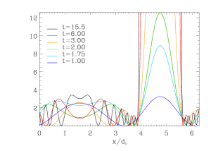
Figure 1: Evolution of $\Pi_{yy}(x,t)$ for ${\bm{B}}=B_{0}{\bm{e}}_{z}$ and constant ${\bm{u}}=(0,V_{0}\cos(x/d_{i}),0)$, $\Omega_{c}\tau_{{}_{H}}=1$ and $V_{0}=1.5c_{{}_{A}}$. Both the exponential growth ($\Omega^{\prime}(x)>0$) and the spatial filamentation of the oscillating solutions ($\Omega^{\prime}(x)<0$) are visible.

,

,

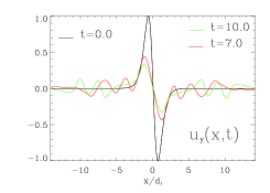
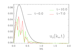
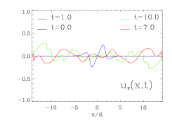
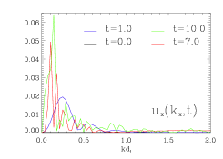
Figure 2: Profiles of $u_{x}(x,t)$ and $u_{y}(x,t)$ (left) and their Fourier spectra (right), for $c_{{}_{H}}=c_{\perp}=c_{{}_{A}}=1$; times in $\tau_{{}_{H}}=\tau_{{}_{B}}$ units.

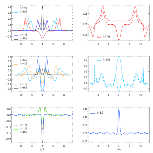
Figure 3: Spatial profiles of the local difference from the initial value for $\delta\Pi_{yy}(x,t)$ (left frames), $\delta\Pi_{xx}(x,t)$ (solid lines, right frames) and $\delta\Pi_{zz}(x,t)$ (three dotted-dashed lines, right). The initial pressures are uniform and isotropic ($\Pi_{ij}^{0}=\delta_{ij}$) with $c_{\perp}/c_{{}_{H}}=1$. As times are in $\tau_{{}_{H}}$ units, the nonlinear waves leave the box earlier in the bottom frames, each row corresponding, from the top down, to $\tau_{{}_{H}}/\tau_{{}_{B}}=c_{{}_{A}}/c_{{}_{H}}=0.1,1$ and $10$ respectively (here $L_{{}_{H}}=d_{i}$).

References

- (1) Talwar, S.P., Phys. Fluids 8, 1295 (1965); N. D’Angelo, Phys. Fluids 8, 1748 (1965).
- (2) Palermo, F., et al., Phys. Plasmas 22, 042304 (2015).
- (3) Stugarek, A., et al., Phys. Rev. Lett. 111, 145001 (2013).
- (4) Chew, G.F., et al., Proc. R. Soc. London A 236, 112 (1956).
- (5) Cerri, S.S., et al., Phys. Plasmas 20, 112112 (2013).
- (6) Astudillo, H.F., et al., AIP Conf. Proc., 382, 289 (1996).
- (7) He, J., et al., Astrophys J Lett., 800:L 31 (2015).
- (8) Posner, A., et al., Geophys. Res. Lett., 30, 6 (2003).
- (9) Marsch, E., et al., J. Geophys. Res.-Space 109, A04120 (2004).
- (10) Zieger, B., at el., Geophys. Res. Lett. 38, L22103 (2011).
- (11) Tu, C.-Y., et al., J. Geophys. Res.-Space 109, A05101 (2004); L. Matteini et al., J. Geophys. Res.-Space 118, 2771 (2013).
- (12) Matteini, L., et al., Space Sci. Rev. 172, 373 (2011).
- (13) Aunai, N., et al., J. Geophys. Res.-Space 116, A09232 (2011); N. Aunai et al., Ann. Geophys. 29, 1571 (2011).
- (14) Scime, E.E., et al., Phys. Plasmas 7, 21 57 (2000).
- (15) Servidio, S., et al., Phys. Rev. Lett. 108, 045001 (2012); D. Perrone et al., Astrophys. J. Lett. 762, 99 (2013).
- (16) Galeotti, L., et al., Phys. Rev. Lett. 95, 015002 (2005).
- (17) André, M., et al., Space Sci. Rev. 80, 27 (1997).
- (18) Yoon, P.H., J. Geophys. Res.-Space 101, 4899 (1996).
- (19) Califano, F. et al., Phys. Rev. Lett. 86, 5293 (2004).
- (20) Califano, F. et al., Phys. Rev. Lett. 96, 105008 (2006).
- (21) Borghesi, M., et al., Phys. Rev. Lett. 80, 5137 (1998); K. Quinn et al., Phys. Rev. Lett. 108, 135001 (2012); W. Fox et al., Phys. Rev. Lett. 111, 225002 (2013).
- (22) Kahn, F.D., J. Fluid Mech. 14, 321 (1962); 19, 210 (1964).
- (23) Albright, N.W., Phys. Fluids 12, 2728 (1970); N. Yajima, Prog. Theor. Phys. 36, 1 (1966).
- (24) Werne, J., et al., Phys. Chem. Earth B 26, 263 (2001).
- (25) Marié, L., et al., Phys. Fluids 16, 457 (2004).
- (26) Hesse, M., et al., Geophys. Res. Lett. 99, 11177 (1994); L. Yin et al., Geophys. Res. Lett. 106, 10761 (2001); L. Yin et al., Phys. Plasmas 10, 1595 (2003).
- (27) Khanna, M., et al., J. Plasma Phys. 28, 459 (1982).
- (28) S.I. Braginskii, in Rev. of Plasma Phys., M.A. Leontovich Ed., Vol.1, p.205, Consultant Bureau, New York (1965).
- (29) Macmahon, A., Phys. Fluids 8, 1840 (1965).
- (30) Passot, T., et al., Phys. Plasmas 11, 5173 (2004); Goswami, P., et al., Phys. Plasmas 12, 102109 (2005).
- (31) Snyder, P.B., et al., Phys. Plasmas 4, 3974 (1997).
- (32) Cerri, S.S., et al., Phys. Plasmas 21, 112109 (2014).
- (33) This is coherent with the definition of the sound velocity in the cold electron limit, where , compatibly with the fact that in our 2D geometry the CGL evolution of is a polytropic with index .
- (34) For example, integration of Eq.(1) in the non-SC case with , and an initially diagonal , gives: , , and .
- (35) Belmont, G., et al., Phys. Plasmas 19, 022108 (2012).