Ordering with precedence constraints and budget minimization

Abstract

We introduce a variation of the scheduling with precedence constraints problem that has applications to molecular folding and production management. We are given a bipartite graph $H=(B,S)$. Vertices in $B$ are thought of as goods or services that must be bought to produce items in $S$ that are to be sold. An edge from $j\in S$ to $i\in B$ indicates that the production of $j$ requires the purchase of $i$. Each vertex in $B$ has a cost, and each vertex in $S$ results in some gain. The goal is to obtain an ordering of $B\cup S$ that respects the precedence constraints and maximizes the minimal net profit encountered as the vertices are processed. We call this optimal value the budget or capital investment required for the bipartite graph, and refer to our problem as the bipartite graph ordering problem.

The problem is equivalent to a version of an NP-complete molecular folding problem that has been studied recently [12]. Work on the molecular folding problem has focused on heuristic algorithms and exponential-time exact algorithms for the un-weighted problem where costs are $\pm 1$ and when restricted to graphs arising from RNA folding.

The present work seeks exact algorithms for solving the bipartite ordering problem. We demonstrate an algorithm that computes the optimal ordering in time $O^{*}(2^{n})$ when $n$ is the number of vertices in the input bipartite graph. We give non-trivial polynomial time algorithms for finding the optimal solutions for bipartite permutation graphs, trivially perfect bipartite graphs, co-bipartite graphs.

We introduce a general strategy that can be used to find an optimal ordering in polynomial time for bipartite graphs that satisfy certain properties. One of our ultimate goals is to completely characterize the classes of graphs for which the problem can be solved exactly in polynomial time.

1 Motivation and Introduction

Job Scheduling with Precedence Constraints

The setting of job scheduling with precedence constraints is a natural one that has been much studied (see, e.g., [5, 15]). A number of variations of the problem have been studied; we begin by stating one. The problem is formulated as a directed acyclic graph where the vertices are jobs and arcs between the vertices impose precedence constraints. Job $j$ must be executed after job $i$ is completed if there is an arc from $j$ to $i$. Each job $i$ has a weight $w_{i}$ and processing time $t_{i}$. A given ordering of executing the jobs results in a completion time $C_{i}$ for each job. Previous work has focused on minimizing the weighted completion time $\sum_{i=1}^{i=n}w_{i}C_{i}$. This can be done in the single-processor or multi-processor setting, and can be considered in settings where the precedence graph is from a restricted graph class. The general problem of finding an ordering that respects the precedence constraints and minimizes the weighted completion time is NP-complete. Both approximation algorithms and hardness of approximation results are known [1, 2, 15, 19].

Our Problem – Optimizing the Budget

In the present work, we consider a different objective than previous works. In our setting, each job $j$ has a net profit (positive or negative) $p_{j}$. Our focus is on the budget required to realize a given ordering or schedule, and we disregard the processing time. We imagine that the jobs are divided between those with negative $p_{i}$, jobs $B$ that must be bought, and jobs with a non-negative $p_{i}$, jobs $S$ that are sold. $B$ could consist of raw inputs that must be purchased in bulk in order to produce goods $S$ that can be sold. A directed graph $H=(B,S)$ encodes the precedence constraints inherent in the production: an arc from $j\in S$ to $i\in B$ implies that item $i$ must be bought before item $j$ can be produced and sold. At each step $1\leq r\leq n$ of the process, let $j_{1},j_{2},...,j_{r}$ be the jobs processed thus far, and let $bg_{r}=\sum_{i=1}^{r}p_{j_{i}}$ be the total budget up to this point. Our goal is an ordering that respects the precedence constraints and keeps the minimal value of $bg_{r}$ as high as possible. One can view (the absolute value of) this optimal value as the capital investment required to realize the production schedule.

In this work we assume $H$ is a bipartite graph with all arcs from $S$ to $B$. This models the situation where each item to be produced and sold depends on certain inputs that must be purchased. We call this the problem of ordering with precedence constraints and budget minimization on bipartite graphs but refer to the problem as the bipartite graph ordering problem.

Applications

The bipartite graph ordering problem is a natural variation of scheduling with precedence constraints problems. As described above the problem can be used to model the purchase of supplies and production of goods when purchasing in bulk. Another way to view the problem is that the items in $B$ are training sessions that employees must complete before employees (vertices in $S$) can begin to work.

We began studying the problem as a generalization of an optimization problem in molecular folding. The folding problem asks for the energy required for secondary RNA structures to be transformed from a given initial folding configuration $\mathcal{C}_{1}$ into a given final folding configuration $\mathcal{C}_{2}$ [8, 14, 18]. The bipartite graph ordering problem models this situation as follows: vertices in $B$ are folds that are to be removed from $\mathcal{C}_{1}$, vertices in $S$ are folds that are to be added, and an edge from $j$ to $i$ indicates that fold $i$ must be removed before fold $j$ can be added. The price $p_{i}$ of a vertex is set according to the net energy that would result from allowing the given fold to occur, with folds that must be broken requiring a positive energy and folds that are to be added given a negative energy. The goal is to determine a sequence of transformations that respects these constraints and still keeps the net energy throughout at a minimum . Figure 1 shows how an instance of the RNA folding problem is transformed into the bipartite graph ordering problem.

Previous Work

The molecular folding problem has been studied only in the setting of unit prices and most attention has been devoted to graph classes corresponding to typical folding patterns (in particular for so-called circle bipartite graphs). [12] shows that the molecular folding problem is NP-complete even when restricted to circle bipartite graphs; thus the bipartite graph ordering problem is NP-complete as well when restricted to circle bipartite graphs .

Previous work on the folding problem has focused on exact algorithms that take exponential time and on heuristic algorithms [7].

Figure 1: The top graph is an instance of the RNA folding problem, with folds $1$, $2$, and $3$ to be removed (bought), folds $a$, $b$, and $c$ to be added (sold); an edge cannot be added until edges that cross it are removed. A budget of two is needed and an optimal ordering is $3$, $2$, $b$, $1$, $a$, $c$.

There has been considerable study of scheduling with precedence constraints, but to our knowledge there has not been any work by that community on the objective function we propose (budget minimization).

1.1 Our Results

We introduce the bipartite graph ordering problem, which is equivalent to a generalization of a molecular folding problem. We initiate the study of which graph classes admit polynomial-time exact solutions. We also give the first results for the weighted version of the problem; previous work on the molecular folding problem assumed unit costs for all folds.

Exponential-time Exact Algorithm

We first give an exact algorithm for arbitrary bipartite graphs.

Theorem 1.1

Given a bipartite graph $H=(B,S)$, the bipartite graph ordering problem on $H$ can be solved in (a) time and space $O^{*}(2^{n})$, and (b) time $O^{*}(4^{n})$ and polynomial space, where $n=|B\cup S|$.

The previous best exact algorithm for the molecular folding problem on circle bipartite graphs has running time $n^{O(K)}$, where $K$ is the optimal budget [18].

We observe that $K$ can be $\Omega(n)$ when vertex prices are $\pm 1$ (and can be much larger when vertex prices can be arbitrary), as follows. Let $\mathcal{P}$ be a projective plane of order $p^{2}+p+1$ with $p$ prime. The projective plane of order $n=p^{2}+p+1$ consists of $n$ lines each consisting of precisely $p+1$ points, and $n$ points which each are intersected by precisely $p+1$ lines. We construct a bipartite graph with each vertex in $B$ corresponding to a line from the projective plane, each vertex in $S$ corresponding to a point from the projective plane, and a connection from $b\in B$ to $s\in S$ if the projective plane point corresponding to $s$ is contained in the line corresponding to $B$. Vertices in $B$ are given weight -1, and vertices in $S$ are given weight 1. Note that the degree of each vertex in $B$ is $p+1$. One can observe that the neighbourhood of every set of $p+1$ vertices in $S$ is at least $p^{2}-{p\choose 2}$. This implies that in order to be able to sell the first $p+1$ vertices in $S$ the budget decreases by at least $p^{2}-{p\choose 2}+p$.

Polynomial-time Cases

We develop algorithms for solving a number of bipartite graph classes. These bipartite graph classes are briefly defined after the theorem statement and discussed further in Sections 5 and 6.

Theorem 1.2

Given a bipartite graph $H=(B,S)$, the bipartite graph ordering problem on $H$ can be solved in polynomial time if $H$ is one of the following: a bipartite permutation graph, a trivially perfect bipartite graph, a co-bipartite graph or a tree.

The bipartite graphs we consider here have been considered for other types of optimization problems. In particular bipartite permutation graphs also known as proper interval bipartite graphs (those for which there exists an ordering of the vertices in $B$ where the neighborhood of each vertex in $S$ is a set of consecutive vertices (interval) and the intervals can be chosen so that they are inclusion free) are of interest in graph homomorphism problems [10] and also in energy production applications where resources (in our case bought vertices) can be assigned (bought) and used (sold) within a number of successive time steps [11, 13]. There are recognition algorithms for bipartite permutation graphs [10, 17]. A bipartite graph is called trivially perfect if it is obtained from a union of two trivially perfect bipartite graphs $H_{1},H_{2}$ or by joining every sold vertex in trivially perfect bipartite graph $H_{1}$ to every bought vertex in trivially perfect bipartite graph $H_{2}$. A single vertex is also a trivially perfect bipartite graph. These bipartite graphs have been considered in [4, 6, 15]. Co-bipartite graphs have a similar definition with a slightly different join operation. See Section 5 for the precise definitions.

For trivially perfect bipartite graphs and co-bipartite graphs, due to the recursive nature of the definition of these graphs it is natural to attempt a divide and conquer strategy. However, a simple approach of solving sub-problems and using these to build up to a solution of the whole problem fails because one may need to consider all possible orderings of combining the sub problems.

In section 7 we develop a general approach that can be applied to the graph classes mentioned.

Arbitrary Vertex Weights

Each of our results holds where the weights on vertices can be arbitrary (not only $\pm 1$ as considered by previous work on the molecular folding problem) except for trees.

2 Some Simple Classes of bipartite graphs

In this section we state some simple facts about the bipartite graph ordering problem and give a simple self-contained proof that the problem can be solved for trees. We provide this section to assist the reader in developing an intuition for the problem.

Bicliques

First we note that if $H$ is a biclique with $|B|=K$ then $bg(H)$ (the budget required to process $H$) is $K$.

As a next step, consider a disjoint union of bicliques $H_{1},H_{2},...,H_{m}$ where each $H_{i}$ is a biclique between bought vertices $B_{i}$ and sold vertices $S_{i}$. Intuition suggests that we should first process those $H_{i}$ such that $|S_{i}|\geq|B_{i}|$. This is indeed correct and is formalized in Lemma 4.6 in Section 4 (the reader is encouraged to take this intuition for granted while initially reading the present section). After processing $H_{i}$ with $|S_{i}|\geq|B_{i}|$, which we call positive (formally defined in generality in Section 4), we are left with bicliques $H_{i}=(B_{i},S_{i})$ where $|B_{i}|>|S_{i}|$. Up to this point we may have built up some positive budget.

In processing the remaining $H_{i}$ the budget steadily goes down – because the $H_{i}$ are bicliques and disjoint, and the remaining sets are not positive. As we shall see momentarily, we should process those $H_{i}$ with largest $|S_{i}|$ first. Suppose on the contrary that $|S_{i}|>|S_{j}|$ but an optimal strategy $opt$ processes $H_{j}$ right before $H_{i}$. If $K$ is the budget before this step we first have that $K-|B_{j}|+|S_{j}|\geq|B_{i}|$ because otherwise there would not be sufficient budget after processing $H_{j}$ to process $H_{i}$. Since we assumed that $|S_{i}|>|S_{j}|$ we have $K-|B_{i}|+|S_{i}|\geq|B_{j}|$. Thus, we could first process $H_{i}$ and then $H_{j}$. We have thus given a method to compute an optimal strategy for a disjoint union of bicliques: first process positive sets, and then process bicliques in decreasing order of $|S_{i}|$.

Paths and Cycles

We next consider a few even easier cases. Note that a simple path can be processed with a budget of at most 2, and a simple cycle can be processed with a budget of $2$.

Trees and Forests

Next we assume the input graph is a tree and the weights are $-1,1$ (for vertices in $B$ and $S$, respectively). Let $H$ be a tree, or in general a forest. Note that any leaf has a single neighbor (or none, if it is an isolated vertex). We can thus immediately process any sold leaf $s$ by processing its parent in the tree and then processing $s$. This requires an initial budget of only 1. After repeating the process to process all sold leaves in $S$, we are left with a forest where all leaves are bought vertices in $B$. We can first remove from consideration any disconnected bought vertices in $B$ (these can, without loss of generality, be processed last). We are left with a forest $H^{\prime}$.

We next take a sold vertex $s_{1}$ (which is not a leaf because all sold leaves in $S$ have already been processed) and process all of its neighbours. After processing $s_{1}$ we can process $s_{1}$ and return 1 unit to the budget. Note that because $H^{\prime}$ is a forest, the neighbourhood of $s_{1}$ has intersection at most 1 with the neighbourhood of any other sold vertex in $S$. Because we have already processed all sold leaves from $H$, we know that only $s_{1}$ can be processed after processing its neighbours.

After processing $s_{1}$, we may be left with some sold leaves in $S$. If so, we deal with these as above. We note that if removing the neighbourhood of $s_{1}$ does create any sold leaves, then each of these has at least one bought vertex in $B$ that is its neighbour and is not the neighbour of any of the other sold leaves in $S$. When no sold leaves remain, we pick a sold vertex $s_{2}$ and deal with it as we did $s_{1}$.

This process is repeated until all of $H^{\prime}$ is processed. We note that after initially dealing with all sold leaves in $S$, we gain at most a single sold leaf at a time. That is, the budget initially increases as we process sold vertices and process their parents in the tree, and then the budget goes down progressively, only ever temporarily going up by a single unit each time a sold vertex is processed. Note that the budget initially increases, and then once it is decreasing only a single sold vertex is processed at a time. This implies that the budget required for our strategy is $|B|-|S|+1$, the best possible budget for a graph with $1,-1$ weights.

3 An Exponential-time Exact Algorithm

In this section we prove Theorem 1.1.

The authors in [3] show that any vertex ordering problem on graphs of a certain form can be solved in both (a) time and space $O^{*}(2^{n})$, and (b) time $O^{*}(4^{n})$ and polynomial space, where $n$ is the number of vertices in the graph and $O^{*}(f(n))$ is shorthand for $O(f(n)\cdot\textnormal{(}poly)(n))$. We show that the ordering problem can be seen to have the form needed to apply this result.

A vertex ordering on graph $H=(B,S)$ is a bijection $\pi:B\cup S\rightarrow\{1,2,\cdots,|B\cup S|\}$. Note that orderings we consider here respect the precedence constraints given by edges of bipartite graph $H$. For a vertex ordering $\pi$ and $v\in B\cup S$, we denote by $\pi_{\prec,v}$ the set of vertices that appear before $v$ in the ordering. More precisely, $\pi_{\prec,v}=\{u\in B\cup S|\pi(u)<\pi(v)\}$.

Let $\Pi(Q)$ be the set of all permutations of a set $Q$ and $f$ be a function that maps each couple consisting of a graph $H=(B,S)$ and a vertex set $Q\subseteq(B\cup S)$ to an integer as follows:

$f(H,Q)=|Q\cap S|-|Q\cap B|$.

Note that the function $f$ is polynomially computable. Now, if we restrict the weights of vertices to be $\pm 1$ (vertices in $B$ have weight -1 and vertices in $S$ have weight 1) we can express the bipartite graph ordering problem as follows:

$bg(H)=\min\limits_{\pi\in\Pi(B\cup S)}\max\limits_{v\in(B\cup S)}f(H,\pi_{\prec,v})$.

The right hand side of this equation is the form required to apply the result of [3], proving Theorem 1.1 for the case of $\pm 1$ weights. The result for arbitrary weights $p_{i}$, with $p_{x}$ negative for $x\in B$ and $p_{y}$ non-negative for $y\in S$, follows by modifying $f(H,Q)$ to be $\sum_{y\in Q\cap S}p_{y}-\sum_{x\in Q\cap B}p_{x}$.

4 Definitions and Concepts

In this section we define key terms and concepts that are relevant to algorithms that solve the bipartite graph ordering problem on general bipartite graph. We use the graph in Figure 2 as an example to demonstrate each of our definitions. The reader is encouraged to consult the figure while reading this section. Recall that bipartite graph $H=(B,S,E)$ encodes the precedence constraints inherent in the production: an arc from $j\in S$ to $i\in B$ implies that item $i$ must be bought before item $j$ can be produced and sold. At each step $1\leq r\leq n$ of the process, let $j_{1},j_{2},...,j_{r}$ be the jobs processed thus far, and let $bg_{r}=\sum_{i=1}^{r}p_{j_{i}}$ be the total budget used up to this point. Our goal is an ordering that respects the precedence constraints and keeps the maximal value of $bg_{r}$ as small as possible.

Let $I$ be a set of vertices. $|I|$ refers to the cardinality of set $I$. When applying our arguments to weighted graphs, with vertex $x$ having price $p_{x}$, we let $|I|$ to be $\sum_{x\in I}|p_{x}|$. Each of our results holds for weighted graphs by letting $|I|$ refer to the weighted sum of prices of vertices in $I$ in all definitions and arguments.

We use $K$ to denote the budget or capital available to process an input bipartite graph. As vertices are processed, we let $K$ denote the current amount of capital available for the rest of the graph.

Definition 4.1

Let $H=(B,S,E)$ be a bipartite graph. For a subset $I\subseteq B$ of bought vertices in $H$, let $N^{*}(I)$ be the set of all vertices in $S$ whose entire neighborhood lie in $I$.

Definition 4.2

We say a set $I\subseteq B$ is prime if $N^{*}(I)$ is non-empty and for every proper subset $I^{\prime}\subset I$, $N^{*}(I^{\prime})$ is empty.

Note that the bipartite graph induced by a prime set $I$ and $N^{*}(I)$ is a bipartite clique. For any strategy to process an input bipartite graph $H$, we look at the budget at each step of the algorithm. Suppose our initial budget is $K$. Knowing which subsets of $B$ are prime, one can see that every optimal strategy can be modified to start with processing a prime subset (Lemma 4.3). This leaves a budget of $K-|I|+|N^{*}(I)|$ to process the rest of the bipartite graph. An example for prime sets is given in Figure 2. For the given graph prime sets are $\{J_{1},J_{2}\}$, $J$, $I$, $I_{1}$ with $N^{*}(\{J_{1},J_{2}\})=D$, $N^{*}(J)=F$, $N^{*}(I)=L$, and $N^{*}(I_{1})=Q$.

Lemma 4.3

There is an optimal strategy for Bipartite Ordering Problem on bipartite graph $H=(B,S,E)$ without isolated vertex, that starts with a prime set.

Proof: Let $\pi$ be an optimal strategy that does not start with a prime set. Suppose $2\leq i\leq n$ is the first position in $\pi$ where $\pi(i)\in S$ and $M=\{\pi(1),\pi(2),\dots,$ $\pi(i-1)\}$. Let set $I\subseteq M$ be the smallest set with $N^{*}(I)\neq\emptyset$. Note that such a set $I$ exists since all the adjacent vertices to $\pi(i)$ are among vertices in $M$. Observe that changing the processing order on vertices in $M$ does not harm optimality. Therefore, we can change $\pi$ by processing vertices in $I$ at first, without changing the budget. In addition, we can process $N^{*}(I)$ immediately after processing $I$. $\diamond$

Our algorithm will generally try to first process subsets $I$ that increase (or at least, do not decrease) the budget. We call such subsets positive, and call $I$ negative if processing it would decrease the budget.

Definition 4.4

A budget of $I\subset B$ is the minimum budget $r$ needed to process $H[I\cup N^{*}(I)]$, denoted by $bg(H[I\cup N^{*}(I)])=r$. For simplicity we write $bg(I)=r$ if $H$ is clear from the context.

Definition 4.5

A set $I\subseteq B$ is called positive if $|I|\leq|N^{*}(I)|$ and it is negative if $|I|>|N^{*}(I)|$. For a given budget $K$, $I$ is called positive minimal (with respect to budget $K$) if it is positive, $I$ has budget at most $K$, and every other positive subset of $I$ has budget more than $K$. In other words, $I$ is smallest among all the subsets of $I$ that is positive and has budget at most $K$.

For the given graph in Figure 2, $I_{1}$ is the only positive minimal set and $N^{*}(I_{1})=O$ contains $7$ vertices. Note that, in general, there can be more than one positive minimal set. Positive minimal sets are key in our algorithms for computing the budget because these are precisely the sets that we can process first, as can be seen from Lemma 4.6. In the graph of Figure 2, the positive set $I_{1}$ would be the first to be processed.

Figure 2: A bipartite permutation graph that we use as an example for the definitions related to our algorithm. Each bold line shows a complete connection, i.e. the induced sub-graph by $I\cup L$ is a biclique. The numbers in the boxes are the number of vertices. The sets $J_{1},J_{2},J,I,I_{1}$ are the items $B$ to be bought, with each vertex having weight -1. The sets $D,E,F,L,P,O$ are the items $S$ to be sold, with each vertex having weight 1.

Lemma 4.6

Let $H=(B,S,E)$ be a bipartite graph that can be processed with budget at most $K$. If $H$ contains a positive minimal set (with respect to $K$) then there is a strategy for $H$ with budget $K$ that begins by processing a positive minimal subset $I$ such that for all $I^{\prime}\subset I$ we have $|N^{*}(I^{\prime})|-|I^{\prime}|\leq|N^{*}(I)|-|I|$.

Proof: Let $I$ be a positive minimal set in $H$. Suppose the optimal process $opt$ does not process $I$ all together and hence processes the sequence $L_{1},I_{1},L_{2},I_{2},\dots,L_{t},I_{t},L_{t+1}$ of disjoint subsets of $B$ where $I=I_{1}\cup I_{2}\cup...\cup I_{t}$ is a positive minimal set and $L_{j}\neq\emptyset$, $2\leq j\leq t$. Note that according to $opt$ for all $L_{i}$, $1\leq i\leq t+1$ we have $bg(L_{i})\leq K-|S_{2}|+|N^{*}(S_{2})|$ in graph $H\setminus S_{2}$ where $S_{2}=\cup_{j=1}^{i-1}L_{j}\cup\cup_{j=1}^{i-1}I_{j}$. First consider the case when $|N^{*}(\cup_{j=1}^{i-1}I_{j})|-|\cup_{j=1}^{i-1}I_{j}|\leq|N^{*}(I)|-|I|$. Let $S_{1}=\cup_{j=1}^{i-1}L_{j}$. For this case we have

$$K-|S_{2}|+|N^{*}(S_{2})| =K-|S_{1}|-|\cup_{j=1}^{i-1}I_{j}|+|N^{*}(S_{2})|$$

$$=K-|S_{1}|+|N^{*}(S_{1})|-|\cup_{j=1}^{i-1}I_{j}|+|N^{*}(\cup_{j=1}^{i-1}I_{j})|+$$

$$|N^{*}(S_{2})\setminus(N^{*}(S_{1})\cup N^{*}(\cup_{j=1}^{i-1}I_{j}))|$$

$$\leq K-|S_{1}|+|N^{*}(S_{1})|-|I|+|N^{*}(I)|+$$

$$|N^{*}(S_{2})\setminus(N^{*}(S_{1})\cup N^{*}(\cup_{j=1}^{i-1}I_{j}))|$$

$$\leq K-|I\cup S_{1}|+|N^{*}(I\cup S_{1})|$$

Therefore $bg(L_{i})$ in graph $H_{1}=H\setminus(I\cup S_{1}\cup N^{*}(I\cup S_{1}))$ is at most $K-|I\cup S_{1}|+|N^{*}(I\cup S_{1})|$. Together with $bg(I)\leq K$, we conclude that, there is another optimal process that considers $I$ first and then $L_{1},L_{2},\dots,L_{t},L_{t+1}$ next and then following $opt$.

Now consider the case when $|N^{*}(\cup_{j=1}^{i-1}I_{j})|-|\cup_{j=1}^{i-1}I_{j}|\geq|N^{*}(I)|-|I|$. Note that since $I$ is a positive minimal set then processing $H[\cup_{j=1}^{i-1}I_{j}\cup N^{*}(\cup_{j=1}^{i-1}I_{j})]$ needs budget more than $K$ as otherwise $\cup_{j=1}^{i-1}I_{j}$ contradicts the minimality of $I$. On the other hand, $opt$ processes $H[S_{2}]$ with budget at most $K$. Therefore, during processing $H[S_{2}]$ there exists a $1\leq\beta\leq i-1$ such that $\cup_{j=1}^{\beta}L_{j}\cup\cup_{j=1}^{\beta}I_{j}$ is a positive set. Minimum such $t$ gives us a positive minimal set. This completes the proof. $\diamond$

Lemma 4.7

Suppose that $I^{+}$ is a positive subset with $bg(I^{+})>K$ and $I^{-}$ is a negative subset where $bg(I^{-})\leq K$ and $I^{+}\cap I^{-}\neq\emptyset$. If $bg(I^{+}\cup I^{-})\leq K$ then $I^{+}\cup I^{-}$ forms a positive subset.

Proof: Let $X=I^{-}\cap I^{+}$. By the assumption that $I^{+}$ can be processed after processing $I^{-}$ we have $bg(I^{+}\setminus X)\leq K-|I^{-}|+|N^{*}(I^{-})|$. On the other hand, since $bg(I^{+})>K$, we have $K-|X|+|N^{*}(X)|<bg(I^{+}\setminus X)$. From these two we conclude that:

$$|N^{*}(I^{-})|>|I^{-}|-|X|$$ (1)

Moreover, because $I^{+}$ is a positive set then $|N^{*}(I^{+})|\geq|I^{+}|$. By (1), $I^{+}$ being positive, and the fact that $|N^{*}(S\cup T)|\geq|N^{*}(S)|+|N^{*}(T)|$ for any $S$ and $T$, we have $|N^{*}(I^{+}\cup I^{-})|\geq|N^{*}(I^{+})|+|N^{*}(I^{-})|\geq|I^{+}|+|I^{-}|-|X|=|I^{+}\cup I^{-}|$, i.e., $I^{+}\cup I^{-}$ is a positive subset. $\diamond$

Given a bipartite graph $H$, Lemma 4.6 suggests a basic strategy, if there are positive sets, find a positive minimal subset $I$, process it. When a given subset $I$ is processed, we would consider the remaining bipartite graph and again try to find a positive minimal subset to process, if one exists. Note that $H\setminus(I\cup N^{*}(I))$ may have positive sets even if $H$ does not. For example, in the graph of Figure 2, $H^{\prime}=(J_{2}\cup J_{1}\cup J,D\cup E\cup F)$ has no positive set, but $J$ is positive in $H^{\prime}\setminus J_{1}$. When a subset $I\subseteq B$ is processed we generally would like to process any sets that are positive in the remaining bipartite graph. That is, we would like to process $c\ell(I)$, defined below. For our purpose we order all the prime sets lexicographically, by assuming some ordering on the vertices of $B$.

Definition 4.8

Given current budget $K$ and given $I\subseteq B$, let $c\ell_{K}(I)=\cup_{i=1}^{r}I_{i}\cup I$ where each $I_{i}\subseteq B$, $1\leq i\leq r$ is the lexicographically first positive minimal subset in $H_{i}=H\setminus(\cup_{j=0}^{i-1}I_{j}\cup N^{*}(\cup_{j=0}^{i-1}I_{j}))$ ($I_{0}=I$) such that in $H_{i}$ we have $bg(I_{i})\leq K-|\cup_{j=0}^{i-1}I_{j}|+|N^{*}(\cup_{j=0}^{i-1}I_{j})|$. Here $r$ is the number of times the process of processing a positive minimal set can be repeated after processing $I$.

When the initial budget $K$ is clear from context, we use $c\ell(I)$ rather than $c\ell_{K}(I)$. Note that $c\ell(I)$ could be only $I$, in this case $r=0$. For instance consider Figure 2. In the graph induced by $\{J,J_{1},J_{2},I,D,E,F,L,P\}$ we have $c\ell(J)=J\cup J_{1}$ with respect to any current budget $K$ at least $12$.

5 Polynomial Time Algorithm for Trivially Perfect Bipartite and Co-bipartite Graphs

In this section we define trivially perfect bipartite graphs and co-bipartite graphs, and discuss the key properties that are used in our algorithm for solving the bipartite graph ordering problem in these bipartite graphs. In particular, it is possible to enumerate the prime sets of these graphs by looking at a way to construct the graphs with a tree of graph join and union operations.

The subclass of trivially perfect bipartite graphs called laminar family bipartite graphs were considered in [16] to obtain a polynomial time approximation scheme (PTAS) for special instances of a job scheduling problem. Each instance of the problem in [16] is a bipartite graph $H=(J,M,E)$ where $J$ is a set of jobs and $M$ is a set of machines. For every pair of jobs $i,j\in J$ the set of machines that can process $i,j$ are either disjoint or one is a subset of the other. The trivially perfect bipartite graphs also play an important role in studying the list homomorphism problem. The authors of [6] showed that for these bipartite graphs, the list homomorphism problem can be solved in logarithmic space. They were also considered in the fixed parametrized version of the list homomorphism problem in [4].

We call these bipartite graphs “trivially perfect bipartite graphs” because the definition mirrors one of the equivalent definitions for trivially perfect graphs.

Definition 5.1 (trivially perfect bipartite graph, co-bipartite graph)

A bipartite graph $H=(B,S,E)$ is called trivially perfect , respectively a co-bipartite graph if it can be constructed by applying the following operations.

• A bipartite graph with one vertex is both trivially perfect and a co-bipartite graph.

• If $H_{1}$ and $H_{2}$ are trivially perfect then the disjoint union of $H_{1}$ and $H_{2}$ is trivially perfect.

  Similarly, the disjoint union of co-bipartite graphs is also a co-bipartite graph.

• If $H_{1}$ and $H_{2}$ are trivially perfect then by joining every sold vertex in $H_{1}$ to every bought vertex in $H_{2}$, the resulting bipartite graph is trivially perfect.

  If $H_{1}$ and $H_{2}$ are co-bipartite graphs, their complete join—where every sold vertex in $H_{1}$ is joined to every bought vertex in $H_{2}$ and every bought vertex in $H_{1}$ is joined to every sold vertex in $H_{2}$—is a co-bipartite graph.

An example of each type of graph is given in Figure 3. In the left figure (trivially perfect) $I=\{I_{1},I_{2}\}$ and $J=\{I_{2},I_{3}\}$ are prime sets. On the right figure (co-bipartite graph) prime sets are $R_{1}=\{J_{1},J_{2},J_{3}\},R_{2}=\{J_{1},J_{2},J_{4}\},R_{3}=\{J_{3},J_{4},J_{1}\},R_{4}=\{J_{3},J_{4},J_{2}\}$ are prime sets.

Figure 3: Each bold line shows a complete connection, i.e. the induced sub-graph by $I_{1}\cup P$ is a biclique.

These two classes of bipartite graphs can be classified by forbidden obstructions, as follows.

Lemma 5.2 ([6, 9])

$H$ is trivially perfect if and only if it does not contain any of the following as an induced sub-graph: $C_{6}$, $P_{6}$.

$H$ is a co-bipartite graph if and only if it does not have any of the followings as an induced sub-graph

Figure 4: Forbidden constructions for co-bipartite graphs.

Our algorithm to solve $bg(H)$ for trivially perfect bipartite graphs and co-bipartite graphs centers around constructing $H$ as in Definition 5.1. We view this construction as a tree of operations that are performed to build up the final bipartite graph, and where the leaves of the tree of operations are bicliques. If $H$ is not connected then the root operation in the tree is a disjoint union, and each of its connected components is a trivially perfect bipartite graph (respectively co-bipartite graph). If $H$ is connected, then the root operation is a join. The following lemma shows how to find such a decomposition tree for given trivially perfect bipartite graph in polynomial time. For co-bipartite graph $H$ a polynomial time algorithm to compute decomposition tree is given in [9].

Lemma 5.3

Given a trivially perfect bipartite graph $H$ with $n$ vertices, there exists an algorithm that finds a decomposition tree for $H$ in time $O(n^{3})$.

Proof: If $H$ is not connected then the root of tree $T$ is $H$ and two children $H_{1},H_{2}$ are chosen such that $H_{1}$ contains all the connected components $H^{\prime}=(B^{\prime},S^{\prime})$ of $H$ where $|B^{\prime}|<|S^{\prime}|$ (if there is any) and $H_{2}$ contains all the other connected components. The root has a label ”union”. Note that if there exists only one such $H^{\prime}$ then $H_{1}=H^{\prime}$. If for every connected component of $H$ the size of its bought vertices is smaller than the size of its sold vertices then one of them would be in $H_{2}$ and the rest lie in $H_{1}$.

If $H$ is connected then we proceed as follows. Let $1\leq m\leq n$ be a maximum integer such that the following test passes. Let $B_{2}$ be the set of vertices in $B$ which have degree at least $m$ and let $B_{1}=B\setminus B_{2}$. Let $S_{1}$ be the set of all vertices in $S$ that are common-neighborhood of all the vertices in $B_{2}$. If $|S_{1}|<m$ then the test fails. Moreover, if there exists a vertex $v\in B_{1}$ such that $N(v)\not\subset S_{1}$ then the tests fails. If the test passes then let $S_{2}=S\setminus S_{1}$ and let the root of $T$ be $H$ with label ”join” and the left child of $H$ is $H[B_{1}\cup N(B_{1})]$ and the right child of the root is $H_{2}=H\setminus H_{1}$. Note that by the definition of trivially perfect bipartite graphs. If the test fails for every $m$ then $H$ is not trivially perfect.

We continue the same procedure from each node of the tree until each node becomes a biclique. Node that $T$ has at most $n$ nodes. For a particular $m$, checking all the conditions of the test takes $O(n)$. Therefore the whole procedure takes $O(n^{3})$. $\diamond$

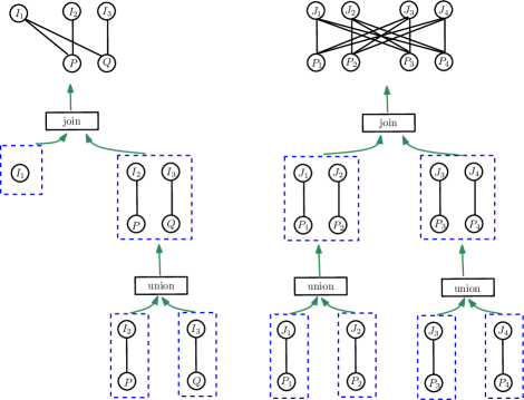
Figure 5: Decomposition tree associated to the graphs in Figure 3.

Algorithm 1 shows that how we traverse a decomposition tree in bottom-up manner and for each node of the tree we do a binary search to find the optimal budget for the graph associated to that node. Note that we assume for the graph associated to a particular node of tree the optimal budgets for its children have been computed and stored.

1:Input: Trivially perfect bipartite (resp.) graph $H=(B,S,E)$, its decomposition tree $T$ 

2:Output: $bg(H)$ 

3:Start from leaves of $T$ and traverse $T$ in bottom-up manner: 

4:Let $H_{x}=(B_{x},S_{x},E_{x})$ be the associated graph to node $x$ of $T$ 

5:$\triangleright$ Assume optimal strategies for children of $H_{x}$ are already computed

6:$l=1$ and $h=|B_{x}|$

7:while  $l\leq h$  do

8:     if BudgetTriviallyPerfect$(H_{x},\lfloor\frac{l+h}{2}\rfloor)$ (resp. BudgetCo-Bipartite) is True then

9:         $h=\lfloor\frac{l+h}{2}\rfloor$  

10:     else

11:         $l=\lfloor\frac{l+h}{2}\rfloor+1$      return l 

Algorithm 1 BudgetTPC ( $H,K$)

If the graph is constructed by union operation it requires a merging function. Such a function is given in Algorithm 6. Combine function takes optimal solutions of two trivially perfect (respectively co-bipartite) graphs and return an optimal strategy for the union of them. In what follows, we give the description of our algorithm and prove its correctness.

Recall that we assume eavery vertex in $B$ has at least one neighbor.

1:Input: Trivially perfect bipartite graph $H=(B,S,E)$ and budget $K$  $\triangleright$ We assume decomposition tree $T$ of $H$ is given.

2:Output: ”True” if we can process $H$ with budget at most $K$, otherwise ”False”. 

3:if $S=\emptyset$ and $K\geq 0$  then return True 

4:if $H$ is a bipartite clique and $|B|\leq K$  then process $H$ by ordering vertices in $B$ first and then ordering vertices in $S$ after and return True 

5:if $H$ is constructed by join operation between $H_{1}=(B_{1},S_{1})$ and $H_{2}=(B_{2},S_{2})$ then $\triangleright$ $bg(H_{1}),bg(H_{2})$ already computed and assume $B_{1}$ and $S_{2}$ induce a bipartite clique.

6:     if  $bg(H_{1})>K$ then return False;

7:     else if $bg(H_{2})>K-|B_{1}|+|S_{1}|$ then return False;

8:     else first process $H_{1}$ then process $H_{2}$ and return True,      

9:if $H$ is constructed by union of $H_{1}$ and $H_{2}$ then

10:     if $\exists$ a positive minimal subset $I$ with $bg(I)\leq K$ then

11:         Process ($I,N^{*}(I)$),

12:         return call BudgetTriviallyPerfect $(H[B\setminus I,S\setminus N^{*}(I)],K-|I|+|N^{*}(I)|)$       

13:     if a positive set $I$ with the smallest budget has $bg(I)>K$  then return False       

14:     if  $bg(H_{1})>K$ OR $bg(H_{2})>K$  then return False 

15:     else return Combine($H_{1},H_{2},K$)      

Algorithm 2 BudgetTriviallyPerfect ($H,K$)

1:Input: Optimal strategies for $H_{1}=(B_{1},S_{1},E_{1}),H_{2}=(B_{2},S_{2},E_{2})$ and budget $K$ 

2:Output: ”True” if we can process $H=H_{1}\cup H_{2}$ with budget at most $K$, otherwise ”False”. 

3:Let $J_{1}$ be the first prime set in $H_{1}$ and $J_{2}$ be the first prime set in $H_{2}$.

4:if $|J_{1}|>K$ OR $bg(H_{2})>K-|c\ell(J_{1})|+|N^{*}(c\ell(J_{1}))|$ then

5:     Process $c\ell(J_{2})$ and $N^{*}(c\ell(J_{2}))$

6:     Call $\textsc{Combine}(H_{1},H_{2}\setminus(c\ell(J_{2})\cup N^{*}(c\ell(J_{2}))),K-|c\ell(J_{2})|+|N^{*}(c\ell(J_{2}))|)$.

7:else

8:     Process $c\ell(J_{1})$ and $N^{*}(c\ell(J_{1}))$,

9:     Call Combine $(H_{1}\setminus(c\ell(J_{1})\cup N^{*}(c\ell(J_{1}))),H_{2},K-|c\ell(J_{1})|+|N^{*}(c\ell(J_{1}))|)$.

Algorithm 3 Combine ( $H_{1},H_{2},K$)

Theorem 5.4

For trivially perfect bipartite graphs $H$ with $n$ vertices the BudgetTriviallyPerfect algorithm runs in $O(n^{2})$ and correctly decides if $H$ can be processed with budget $K$ (Algorithm 2).

Proof: The correctness of lines 3,4 is obvious. It is clear that if $H$ is obtained from $H_{1}$ and $H_{2}$ by join operation then the any optimal strategy must starts with $H_{1}$. Therefore the Lines 5–8 are correct.

Suppose $H$ is obtained from $H_{1},H_{2}$ by union operation. Let $I$ be a positive minimal set and let $H^{\prime}$ be the induced sub-graph of $H$ by $I\cup N^{*}(I)$. If $H^{\prime}$ is not connected then there is at least one connected component of $H^{\prime}$ that is positive, a contradiction to minimality of $I$. Thus we may assume $H^{\prime}$ is connected. According to the decomposition of $H^{\prime}$ there are $H^{\prime}_{1}=(B^{\prime}_{1},S^{\prime}_{1})$ and $H^{\prime}_{2}=(B^{\prime}_{2},S^{\prime}_{2})$ such that $H^{\prime}_{1}$ and $H^{\prime}_{2}$ are trivially perfect bipartite graph. Suppose every bought vertex in $B^{\prime}_{1}$ is adjacent to every sold vertex in $S^{\prime}_{2}$. Observe that any positive set must include either a positive part of $H^{\prime}_{1}$ or all $H^{\prime}_{1}$ together with a positive part of $H^{\prime}_{2}$. In the former case, we search in $H^{\prime}_{1}$ for a positive set. In the later one, we search for a positive set $I^{\prime}$ in $H^{\prime}_{2}$ so that $|N^{*}(I^{\prime})|-|I^{\prime}|\geq|B^{\prime}_{1}|-|S^{\prime}_{1}|$. In either case, we repeat the same procedure and traverse the decomposition tree to find a positive set. This takes $O(n^{2})$. The correctness of Lines 10-12 is followed by Lemma 4.3 and 4.6. Suppose line 13 is incorrect and all positive subsets would have budget above $K$. Let $I^{+}$ be one such subset. Then there would be a way to process $I^{+}$ with budget at most $K$ in $H$. In that case, we would process some negative set $I^{-}$ which somehow reduces the budget of processing $I^{+}$; this can only be so if $I^{-}\cap I^{+}\neq\emptyset$. In this case the Lemma 4.7 states that $I^{+}\cup I^{-}$ is itself a positive set with budget at most $K$, a contradiction.

We continue our argument by assuming that $H$ is constructed form $H_{1}=(B_{1},S_{1})$ and $H_{2}=(B_{2},S_{2})$ by ”union” operation. We proceed by showing the correctness of Combine function. Let $J_{1}$ be the first prime set in $H_{1}$ and $J_{2}$ be the first prime set in $H_{2}$.

Observation 5.5

Let $H_{1}=(B_{1},S_{1})$ and $H_{2}=(B_{2},S_{2})$ be two disjoint trivially perfect bipartite graphs ($H_{1}\cap H_{2}=\emptyset$). Suppose optimal strategies for computing the budget for $H_{1}$ and $H_{2}$ are provided. If $J_{1},J_{2}$ are the first prime sets in $H_{1},H_{2}$ then there is an optimal ordering for $H=H_{1}\cup H_{2}$ such that either $c\ell(J_{1})$ or $c\ell(J_{2})$ is processed first.

To complete the proof for correctness of Combine function, it remains to show that the Combine function correctly chooses between $J_{1}$ and $J_{2}$, the first prime set to process in $H$. Suppose we have $|J_{1}|<K$ and $bg(H_{2})\leq K-|c\ell(J_{1})|+|N^{*}(c\ell(J_{1}))|$. We claim there exists an optimal strategy for $H$ that starts processing $c\ell(J_{1})$ first. Let $opt$ be the optimal strategy that process $c\ell(J_{2})$ first. Let $J_{2},J_{3},\dots,J_{k}$ be the prime subsets in $H_{2}$ that are processed by $opt$ before starting $J_{1}$ in $H_{1}$ (note that by Observation above $opt$ starts processing $c\ell(J_{1})$ in $H_{1}$ first). We note that $bg(H_{2})\geq bg(J_{2}\cup J_{3}\cup\dots\cup J_{k})$. Because we assume that there is no positive set in $H_{2}$. Therefore we have $K-|c\ell(J_{1})|+|N^{*}(c\ell(J_{1}))|\geq bg(H_{2})\geq bg(J_{2}\cup J_{3}\cup\dots\cup J_{k})$ and hence we obtain a strategy $opt^{\prime}$ that starts with $c\ell(J_{1})$ first and then it processes $J_{2},J_{3},\dots,J_{k}$ from $H_{2}$ and then it follows $opt$. Observe that under $opt^{\prime}$, $bg(H)$ does not increases.

Note that finding $c\ell(J)$ takes $O(n)$ and it can be determined according to join or union operation as follows.

Suppose $H$ is associated to a node of the decomposition tree and it is constructed from $H_{1}$ and $H_{2}$ either by union or join operation. Without loss of generality, we assume there is no positive minimal set in $H$, as otherwise, we process them first. Let $c\ell(J)\subseteq B_{1}$. First, if the operation is union then $c\ell(J)$ does not change. Second, suppose the operation is join and every sold vertex in $H_{2}$ is adjacent to every bought vertex in $H_{1}$. If $c\ell(J)$ is the entire $B_{1}$ then $c\ell(J)$ is $B_{1}$ plus all positive minimal sets in $H_{2}$. If $c\ell(J)\subset B_{1}$ then it does not change in $H$. Therefore, updating $c\ell(J)$ at each step takes at most $O(n)$ time. These would imply that the overall running time would be $O(n^{2})$. $\diamond$

In what follows we show that there is a subclass of trivially perfect bipartite graphs that are also circle bipartite graphs. A bipartite graph $H=(B,S,E)$ is called a chain graph if the neighborhoods of vertices in $B$ form a chain, i.e, if there is an ordering of vertices in $B$, say $w_{1},w_{2},\cdots,w_{p}$, such that $N(w_{1})\supseteq N(w_{2})\supseteq\cdots\supseteq N(w_{p})$.

It is easy to see that the neighborhoods of vertices in $S$ also form a chain. Chain graphs are subsets of both trivially perfect bipartite graphs and circle bipartite graphs. Any chain graph can be visualized as what is depicted in Figure 6(a), and the corresponding RNA model for the bipartite graph ordering problem looks like Figure 6(b).

Figure 6: $(a)$: Each bag $B_{i}$ and $S_{i}$ contains at least one vertex, for $1\leq i\leq 4$. A line between $B_{i}$ and $S_{j}$ means that vertices in $B_{i}\cup S_{j}$ induce a complete bipartite graph for $1\leq i,j\leq 4$. $(b)$ : Each $B_{i}$ and $S_{i}$ arc represents a collection of arcs; the number of arcs which are represented by each $B_{i}$ and $S_{j}$ arc is equal to the number of vertices in bag $B_{i}$ and $S_{i}$, for $1\leq i,j\leq 4$.

Next we present a polynomial time algorithm for co-bipartite graphs. Our algorithm for this class of graphs is quite similar to Algorithm 2. The main difference is in the way we deal with co-bipartite graph $H=(B,S,E)$ when it is constructed from two co-bipartite graphs $H_{1}=(B_{1},S_{1},E_{1})$ and $H_{2}=(B_{2},S_{2},E_{2})$ by join operation. Recall that in join operation for co-bipartite graphs, $H[B_{1}\cup S_{2}]$ and $H[B_{2}\cup S_{1}]$ are bipartite cliques. Observe that in this case there are two possibilities for processing $H$:

• first process entire $B_{2}$ then solve the problem for $H_{1}$ with budget $K-|B_{2}|$, and at the end process $S_{2}$, or

• first process entire $B_{1}$ then solve the problem for $H_{2}$ with budget $K-|B_{1}|$, and at the end process $S_{1}$.

For the case when $H$ is constructed from $H_{1}$ and $H_{2}$ by union operation we call Combine function (Algorithm 6). The description of our algorithm is given in Algorithm 4. The proof of correctness of Algorithm 4 is almost identical to the proof of Theorem 5.4.

Theorem 5.6

Algorithm 4 in polynomial times decides if co-bipartite graph $H$ can be processed with budget at most $K$.

1:Input: Co-bipartite graph $H=(B,S,E)$ constructed from $H_{1}=(B_{1},S_{1},E_{1})$ and $H_{2}=(B_{2},S_{2},E_{2})$, $bg(H_{1})$, $bg(H_{2})$, its decomposition tree $T$, and budget $K$ 

2:Output: ”True” if we can process $H$ with budget at most $K$, otherwise ”False”. 

3:if $S=\emptyset$ and $K\geq 0$ OR $H$ is a bipartite clique and $|B|\leq K$ then process $H$ and return True 

4:if $H$ is constructed by join operation between $H_{1}$ and $H_{2}$ then

5:     if  $bg(H_{1})\leq K-|B_{2}|$  then return True and process $B_{2}$, process $H_{1}$ with     budget $K-|B_{2}|$, and process $S_{2}$ 

6:     else if  $bg(H_{2})\leq K-|B_{1}|$  then return True and process $B_{1}$, process $H_{2}$ with     budget $K-|B_{1}|$, process $S_{1}$ 

7:     else return False       

8:if $H$ is constructed by union of $H_{1}$ and $H_{2}$ then

9:     if $\exists$ a positive minimal subset $I$ with $bg(I)\leq K$ then

10:         Process $I$ and $N^{*}(I)$,

11:         return call BudgetCo-Bipartite $(H[B\setminus I,S\setminus N^{*}(I)],K-|I|+|N^{*}(I)|)$       

12:     if a positive set $I$ with the smallest budget has $bg(I)>K$  then return False       

13:     if  $bg(H_{1})>K$ OR $bg(H_{2})>K$ then return False 

14:     else return Combine( $H_{1},H_{2},K$)      

Algorithm 4 BudgetCo-Bipartite ($H,K$)

6 Polynomial Time Algorithm for Bipartite Permutation Graphs

A bipartite graph $H=(B,S,E)$ is called permutation graph (proper interval bipartite graph) if there exists an ordering $<$ of the vertices in $B$ such that the neighborhood of each vertex in $S$ consists of consecutive vertices in $<$. Moreover, for any two vertices $s_{1},s_{2}\in S$ if $N(s_{1})\subset N(s_{2})$ then the last neighbor of $s_{1}$ and the last neighbor of $s_{2}$ are the same. These bipartite graphs were exactly those bipartite graph for which the minimum cost homomorphism problem can be solvaled in polynomial time [10]. They are also studied in job scheduling problems [11, 13].

We refer to a set of consecutive vertices in such an ordering as an interval. Figure 2 is an example of a bipartite permutation graph.

Note that the class of circle bipartite graphs $G=(X,Y)$, for which obtaining the optimal budget is NP-complete, contains the class of bipartite permutation graphs.

We obtain an ordering $<$ for vertices in $S$ by setting $s<s^{\prime}$ if the first neighbor of $s$ is before the first neighbor of $s^{\prime}$ in $<$ as therwise $s^{\prime}<s$. Let $b_{1},b_{2},\dots,b_{p}$ and $s_{1},s_{2},\dots,s_{q}$ be the orderings of $B$ and $S$ respectively. If $s_{i}b_{j}$ and $s_{i^{\prime}}b_{j^{\prime}}$ are edges of $H$ and $j^{\prime}<j$ and $i<i^{\prime}$ then $s_{i}b_{j^{\prime}},s_{i^{\prime}}b_{j}\in E(H)$. Such an ordering is called min-max ordering [10].

Let $B[i,j]$ denote the interval of vertices $b_{i},b_{i+1},\dots,b_{j}$. In the Algorithm 5 we compute the optimal budget for every $B[i,j]$. In order to compute $bg(B[i,j])$ we assume that the optimal strategy starts with some sub-interval $J$ of $B[i,j]$ and it processes $c\ell(J)$. Then we are left with two disjoint instances $B_{1},B_{2}$ (this is because of property of the min-max ordering). We then argue how to combine the optimal solutions of $B_{1}$ and $B_{2}$ and obtain an optimal strategy for $B[i,j]\setminus c\ell(J)$. We need to consider every possible prime interval $J$ in range $B[i,j]$ and take the minimum budget.

1:Input: Bipartite permutation graph $G=(B,S,E)$ with ordering $<$ on vertices in $B,S$ i.e. $b_{1}<b_{2}<\dots<b_{n},s_{1}<s_{2}<\dots<s_{m}$ 

2:Output: Computing the budget for $G$ and optimal strategy 

3:for  $i=1$ to $i=n-1$  do

4:     for  $j=1$ to $j\leq n-i$ do

5:         Let $H^{\prime}=(B[j,j+i],N^{*}(B[j,j+i]))$

6:         Let $K^{\prime}$ be the minimum number s.t. Optimal-Budget($H^{\prime},K^{\prime}$) is True.

7:         Set $bg(H^{\prime})=K^{\prime}$ and let process of $H^{\prime}$ be according to Optimal-Budget($H^{\prime},K^{\prime}$)

8:         Let $H_{r}=H^{\prime}\cup S_{r}$ ($S_{r}$ is the set of vertices who have neighbors in both $B[j+1,n],B[i,j]$)

9:         Let $K^{\prime}$ be the minimum number s.t. Optimal-Budget($H_{r},K^{\prime}$) is True.

10:         Set $bg(H_{r})=K^{\prime}$ and let process of $H_{r}$ be according to Optimal-Budget($H_{r},K^{\prime}$)

11:         Let $H_{l}=H^{\prime}\cup S_{l}$ ($S_{l}$ is the set of vertices who have neighbors in both $B[1,i-1],B[i,j]$)

12:         Let $K^{\prime}$ be the minimum number s.t. Optimal-Budget($H_{l},K^{\prime}$) is True.

13:         Set $bg(H_{l})=K^{\prime}$ and let process of $H_{l}$ be according to Optimal-Budget($H_{l},K^{\prime}$)      

14:

15:function Optimal-Budget($H=(B,S)$, $K$)

16:     Input: Bipartite permutation graph $H=(B,S,E)$ with ordering $<$ on vertices in $B,S$

17:     Output: Process $H$ with budget at most $K$, otherwise ”False”. 

18:     if $S=\emptyset$ and $K\geq 0$ OR $H$ is a bipartite clique and $|B|\leq K$ then return Process $H$       

19:     if there is a positive minimal subset $I$ with $bg(I)\leq K$ then process $I$ and $N^{*}(I)$

20:         return BudgetPermutation $(H[B\setminus I,S\setminus N^{*}(I)],K-|I|+|N^{*}(I)|)$       

21:     if  $|I|>K$ for all prime $I\subseteq B$ then return False       

22:     if a positive set $I$ with the smallest budget has $bg(I)>K$  then return False       

23:     for  every prime interval $I$ of $H$  do

24:         Let $H_{1}=(B_{1},S_{1})$ and $H_{2}=(B_{2},S_{2})$ where $B_{1}=\{b_{1},b_{2},\dots,b_{i}\}$ and $B_{2}=\{b_{j},\dots,b_{n}\}$    $b_{i+1}$ is the first vertex of $c\ell(I)$ and $b_{j-1}$ is the last vertex of $c\ell(I)$ in the ordering $<$

25:         Let $S_{i}$, $i=1,2$ be the set of vertices in $S$ that have neighbors in $B_{i}$ $\triangleright$ $S_{1}\cap S_{2}=\emptyset$ 

26:         Set Flag=Combine($H_{1},H_{2},K-|c\ell(I)|+|N^{*}(c\ell(I))|$).

27:         if  Flag=True then

28:              Process of $H$ be $c\ell(I)$ together with process of $H\setminus(c\ell(I)\cup N^{*}(c\ell(I)))$ by Combine

29:              return               

Algorithm 5 BudgetPermutation ( $H,K$)

1:Input: Optimal strategies for $H_{1}=(B_{1},S_{1},E_{1}),H_{2}=(B_{2},S_{2},E_{2})$ and budget $K$ 

2:Output: ”True” if we can process $H=H_{1}\cup H_{2}$ with budget at most $K$, otherwise ”False”. 

3:Let $J_{1}$ be the first prime set in $H_{1}$ and $J_{2}$ be the first prime set in $H_{2}$.

4:if $|J_{1}|>K$ OR $bg(H_{2})>K-|c\ell(J_{1})|+|N^{*}(c\ell(J_{1}))|$ then

5:     Process $c\ell(J_{2})$ and $N^{*}(c\ell(J_{2}))$

6:     Call $\textsc{Combine}(H_{1},H_{2}\setminus(c\ell(J_{2})\cup N^{*}(c\ell(J_{2}))),K-|c\ell(J_{2})|+|N^{*}(c\ell(J_{2}))|)$.

7:else

8:     Process $c\ell(J_{1})$ and $N^{*}(c\ell(J_{1}))$,

9:     Call Combine $(H_{1}\setminus(c\ell(J_{1})\cup N^{*}(c\ell(J_{1}))),H_{2},K-|c\ell(J_{1})|+|N^{*}(c\ell(J_{1}))|)$.

Algorithm 6 Combine ( $H_{1},H_{2},K$)

Theorem 6.1

Algorithm 5 solves the Bipartite Ordering Problem on a bipartite permutation graph with $n$ vertices in time $O(n^{6}\log|B|)$.

Proof: Let $H=(S,B,E)$ be a bipartite permutation graph with an ordering on its vertices as described above. We use a dynamic programming table which keeps track of the the subgraph $H^{\prime}$ induced by $B[i,j],N^{*}(B[i,j])$ and $b_{i},b_{i+1},\dots,b_{j}$ is an interval in $B$. In the table we also keeps track of the subgraph $H^{\prime\prime}=(B^{\prime\prime},S^{\prime\prime})$ where $B^{\prime\prime}$ is a sub-interval of $B$ and $S^{\prime\prime}$ consists of vertices $N^{*}(B^{\prime\prime})$ together with vertices of $S$ that are not initially in $N^{*}(B^{\prime\prime})$ but are initially in $N^{*}(B^{\prime\prime}\cup J)$ where $N(B^{\prime\prime})\cap N(J)\neq\emptyset$ for some sub-interval $J$ of $B$. This instances appears after removing $c\ell(I)$ for some prime intervals $I$ of $B$. The number of such sub-instance is at most $O(n)$ for each interval $I$ of $B$.

Now we show that Function Optimal-Budget correctly compute the budget for a given instance. The line 19 of the function is obvious. The correctness of lines 20-23 follow from Lemmas 4.3, 4.6, and Lemma 4.7.

We show how to find an optimal ordering for $H$ following the rules of Function Optimal-Budget. First, we need to find all positive minimal sets. For bipartite permutation graphs, prime sets, the closure of a prime set ($c\ell(I)$), and any positive minimal set is an interval.

Note that computing $c\ell(I)$ takes $O(n)$ and it is a straightforward procedure. Once $I$ is removed from $B$ there are two unique prime intervals (one on the right of $I$ and one in the left of $I$) that could potentially become positive and it can be added into $c\ell(I)$.

When we consider processing a positive minimal set, we not that according to Definition 4.5, it does not have any proper positive subset. Therefore, it is the same as the case when we have a bipartite permutation graph without any positive prime interval and no positive closure set (Definition 4.8).

Now suppose there is no positive prime interval. The optimal strategy starts with some prime interval $I$ and then it process the closure of that interval. After removing $c\ell(I)$ and $N^{*}(c\ell(I))$ we end up with two instances $H_{1}=(B_{1},S_{1})$ and $H_{2}=(S_{2},B_{2})$ where they are disjoint. Note that no vertex $s\in S_{2}$ is adjacent to any vertex in $b\in B_{1}$ as otherwise the vertices in $N^{*}(c\ell(I))$ must be adjacent to $b$ (because of the min property of the min-max ordering $<$) which are not adjacent. No vertex $s^{\prime}\in S_{1}$ is adjacent to any vertex $b^{\prime}\in B_{2}$ as otherwise the vertices in $N^{*}(c\ell(I))$ must be adjacent to $b^{\prime}$ (because of the max property of min-max ordering) which are not adjacent.

Now by similar argument as in the proof of Theorem 5.4 we conclude that Combine obtain an optimal strategy for $H_{1}\cup H_{2}$, given the optimal strategy for $H_{1}$ and $H_{2}$. Observe that in the algorithm we consider every possible interval $I$ therefore we obtain an optimal strategy to compute $bg(H)$. For a prime set $J$, computing the $c\ell(J)$ takes $O(n)$. Combine algorithm takes $O(n^{2})$ to obtain the strategy for $H_{1}\cup H_{2}$ (because at each steps it computes $c\ell(J_{i})$, $i=1,2$ for the primes intervals in $H_{1},H_{2}$).

For each interval $I$ of $B$ we call the Function Optimal-Budget at most three times. In Function Optimal-Budget we call the Combine function at most $O(|I|^{2})$ times (there are at most $O(|I|^{2})$ prime intervals). Therefore the running time of Function Optimal-Budget is $O(|I|^{4})$ and it is at most $O(n^{4})$. There are at most $n^{2}$ intervals. Therefore the running time of Algorithm 5 is $O(n^{6}\log|B|)$. The term $\log|B|$ is because we should binary search to obtain the optimial value $K^{\prime}$ in lines 9,12.

$\diamond$

7 General Strategy

It may not always be the case that all positive sets can be identified in polynomial time. But, if positive sets can be identified, the following is a general strategy for processing an input bipartite graph $H$ and given budget $K$.

1. If there exist positive sets in $B$, process a positive minimal set $I$, set $H=(B\setminus I,S\setminus N^{*}(I))$, update $K$ to $K-|I|+|N^{*}(I)|$ and repeat step 1.

2. If no positive set exists, choose in some way the next prime set $I$ to process, set $H=(B\setminus I,S\setminus N^{*}(I))$, update $K$ to be $K-|I|+|N^{*}(I)|$ and go to step 1.

Note that each time a prime set $I$ is processed, we end up processing $c\ell(I)$. Even if we can identify the prime and positive sets, it remains to determine in the second step the method for choosing the next prime to process. We address this issue and give the full algorithm and proof for Theorem 1.2 in the next subsection. Note that Lemma 4.6 implies that without loss of generality we can assume that when a prime set $I$ is processed the remainder of $c\ell(I)$ is processed next, as it is stated in the next corollary.

Corollary 7.1

Let $H=(B,S)$ be a bipartite graph that can be processed with budget at most $K$ with an ordering that processes prime set $I$ first. Then there is a strategy for $H$ that processes $c\ell(I)$ first and uses budget at most $K$.

7.1 Algorithm and Correctness of Proof for Theorem 1.2

In this section we give the algorithm and proof for Theorem 1.2, that we can solve the bipartite graph ordering problem for some classes of graphs. From the previous section it remains to determine how to choose which prime set to process first when there are no positive sets that can be processed.

Definition 7.2

Let $I,J$ be prime subsets. We say that $I$ is potentially after $J$ for current budget $K$ if

1. $|I|>K$, or

2. $bg(c\ell(J)\setminus c\ell(I))>K-|c\ell(I)|+|N^{*}(c\ell(I))|$

Definition 7.2 is a first attempt at choosing which prime set to process first. The idea is to consider whether it is possible to process $I$ before $J$. Item 2 in the definition states that $J$ could not be processed immediately after $I$. However, this formula is not sufficient in general because we must consider orderings that do not process $I$ and $J$ consecutively, and we must take into account that for whatever ranking we define on the prime sets the ranking may change as the algorithm processes prime sets. For clarification we have singled out the case when $I$ and $J$ are processed consecutively in the proof of correctness of the algorithm.

If two prime sets $I$ and $J$ are not processed consecutively by the $opt$ strategy, we should adapt Item 2 of Definition 7.2 to take into account all vertices that would be processed in between by our algorithm. We call this set of vertices the “Superset” of $J$ with respect to $I$, defined precisely by the recursive Definitions 7.3 and 7.4.

Definition 7.3

Let $I$ and $J$ be two prime subsets. For current budget $K$, the Superset of $J$ with respect to $I$, denoted as $Superset_{I}(J)$, is defined as follows. $Superset_{I}(J)$ contains $c\ell(J)$ and at each step a set $c\ell(J_{i})$ is added into $Superset_{I}(J)$ from $B\setminus Superset_{I}(J)$ where $J_{i}$ is first according to the lexicographical order of prime sets such that no prime set is before $J_{i}$ according to the ordering in Definition 7.4. We stop once $c\ell(I)$ lies in $Superset_{I}(J)$.

Definition 7.4

For current budget $K$, we say prime subset $I$ is after prime subset $J$ if

1. $|I|>K$, or

2. $bg(Superset_{I}(J)\setminus c\ell(I))>K-|c\ell(I)|+|N^{*}(c\ell(I))|$

Definition 7.4 states that $I$ is after $J$ if it is too large for the current budget (Item 1) or cannot be processed before $J$ using the ordering implied by Definitions 7.3 and 7.4 (Item 2). Note that if $I$ is processed right after $c\ell(J)$ then Item 2 in Definition 7.4 agrees with Definition 7.2. In the graph induced by $\{J,J_{1},J_{2},I,D,E,F,L,P\}$ in Figure 2, we have $Superset_{I}(J)=J\cup J_{1}\cup J_{2}$ with respect to any current budget $K$ at least 12.

We point out that Definitions 7.3 and 7.4 are recursive, and a naive computation of the ranking would not be efficient. We describe how to efficiently compute the ranking for the classes of graphs of Theorem 1.2 using dynamic programming in Sections 5 and 6. The main description of our general strategy is given in Algorithm 7.

1:Input: $H=(B,S,E)$ and budget $K$ 

2:Output: ”True” if we can process $H$ with budget at most $K$, ”False” otherwise. 

3:if $S=\emptyset$ and $K\geq 0$ then return True 

4:if  $|I|>K$ for all prime $I\subseteq B$ then return False 

5:if there is a positive minimal subset $I$ with $bg(I)\leq K$ then return Budget $(H[B\setminus I,S\setminus N^{*}(I)],K-|I|+|N^{*}(I)|)$ 

6:if a positive set $I$ with the smallest budget has $bg(I)>K$  then return False 

7:Let $I$ be the lexicographically first prime subset with no other prime set before it according to ordering in Definition 7.4.

8:if no such $I$ exists then return False

9:else return Budget $(H[B\setminus I,S\setminus N^{*}(I)],K-|I|+|N^{*}(I)|)$ 

Algorithm 7 Budget ( $H=(B,S,E)$, $K$)

The algorithm determines whether $bg(H)\leq K$. Note that the exact optimal value can be obtained by using binary search, and since the optimal value is somewhere between 0 and $|B|$ the exact computation is polynomial if the decision problem is polynomial.

Before considering the running time for the graph classes of Theorem 1.2 we first demonstrate that the algorithm in Algorithm 7 decides correctly, though possibly in exponential time, for any instance $(H=(B,S),K)$.

Lemma 7.5

For any $K$ and bipartite graph $H$, the Budget algorithm (Algorithm 7) correctly decides if $bg(H)\leq K$ or not.

Proof: We show that if $bg(H)=K$ then there exists an optimal solution $opt^{\prime}$ with budget $K$ in which subset $I$ as described in the algorithm is processed first. We use induction on the size of $B$, meaning we assume that for smaller instances, there is an optimal process that considers the prime subsets according to the rules of our algorithm.

Correctness of Lines 3 is clear and the correctness of line 4 follows from Lemma 4.3. The correctness of steps 5 follows from Lemma 4.6. Suppose Line 6 were incorrect. Then all positive subsets would have budget above $K$. Let $I^{+}$ be one such subset and yet if Line were incorrect there would be a way to process $I^{+}$ with budget at most $K$ in $H$. In that case, we would process some negative set $I^{-}$ which somehow reduces the budget of processing $I^{+}$; this can only be so if $I^{-}\cap I^{+}\neq\emptyset$. In this case the Lemma 4.7 states that $I^{+}\cup I^{-}$ is itself a positive set with budget at most $K$, a contradiction to the premise of step 6.

We are left to verify Lines 7-9, so we continue by assuming there are no positive subsets. Let $I$ be the first prime set according to Definition 7.4. Suppose for the sake of contradiction that the optimal solution $opt$ processes prime subset $J$ before $I$. In what follows we show that we can modify $opt$ and process $I$ as the first prime set. Note that, since there is no positive subset at the beginning, $opt$ processes $c\ell(J)\setminus J$ after $J$.

Suppose that by induction hypothesis (rules of our algorithm) the $opt$ would place $I\setminus c\ell(J)$ first in $H^{\prime}=(B\setminus c\ell(J),S\setminus N^{*}(c\ell(J)))$. In this case $Superset_{I}(J)\setminus c\ell(I)$ is just $c\ell(J)\setminus c\ell(I)$, and in this case Definitions 7.2 and 7.4 coincide.

We show that we can modify $opt$ to process $c\ell(I)$ first and then $J\setminus c\ell(I)$ next while still using budget at most $K$. Suppose this is not the case. Now we have the following

• $bg(c\ell(J)\setminus c\ell(I))>K-|c\ell(I)|+|N^{*}(c\ell(I))|$

The inequality (a) follows from the assumption that we cannot process $c\ell(I)$ first and then immediately processing $J\setminus c\ell(I)$. However, this is a contradiction to the fact that $I$ is before $J$ according to Definition 7.4.

We also note that since $bg(c\ell(J))\leq bg(Superset_{I}(J)\setminus c\ell(I))\leq K-|c\ell(I)|+|N^{*}(c\ell(I))|$, we can also process the entire $c\ell(J)$ after processing $c\ell(I)$. Therefore we can exchange processing $c\ell(I)$ with $c\ell(J)$ and follow the $opt$ in the remaining.

We are left with the case that $c\ell(J)$ is processed first by $opt$, and the rules of the algorithm (second item in Definition 7.4) would process some prime subset $L$ different from $I\setminus c\ell(J)$ next. This would imply that there is some prime subset $L$ that is considered before the last remaining part of $I$ in $B\setminus c\ell(J)$. By induction hypothesis we may assume that the $opt$ processes the prime subsets according to the second item in Definition 7.4. These would imply $L$ is in $Superset_{I}(J)$. At some point $I$ or the remaining part of $I$ becomes the first set to process according to the rules of the algorithm and this happens at the last step of the definition of $Superset_{I}(J)$. However, since there is no other prime subset before $I$ according to Definition 7.4 we have $bg(Superset_{I}(J)\setminus c\ell(I))\leq K-|c\ell(I)|+|N^{*}(c\ell(I))|$. Therefore we can process $c\ell(I)$ first and next $c\ell(J)\setminus c\ell(J)$ and then follow $opt$.

It remains to show that if $bg(H)\leq K$ then there exists a prime subset $I$ that is the lexicographically first prime subset with no other prime set before it according to the ordering in Definition 7.4. Suppose there exists an ordering for $H$ with budget at most $K$ as follows: $c\ell(J),c\ell(J_{1}),\dots,c\ell(J_{r})$. By induction assume that the Budget Algorithm returns “true” for instance $H\setminus\{c\ell(J)\cup N^{*}(c\ell(J))\}$ with budget $K-|c\ell(J)|+|N^{*}(c\ell(J))|$ and the output ordering is $c\ell(J_{1}),\dots,c\ell(J_{r})$. Therefore, by Definition 7.3, $Superset_{J_{i}}(J)=\cup_{t=1}^{i}c\ell(J_{t})$ for $1\leq i\leq r$. Observe that $J$ is not after any prime subset by Definition 7.4 which leads us to have $J$ as a valid “first” prime subset in $H$ for the algorithm. $\diamond$

A naive implementation of the algorithm would consider all possible orderings of prime sets to determine the ordering in step 4 of the algorithm, and in the worst-case an exponential number of sets may need to be considered to identify the prime and positive minimal sets. A careful analysis can be taken to show that the running time of the algorithm in the general case is exponential. In the next two sections we show that for the graph classes of Theorem 1.2 the running time is polynomial.

8 Future Work and Open Problems

We have defined a new scheduling or ordering problem that is natural and can be used to model processes with precedence constraints. As with any optimization problem there are many avenues of attack. In this work we have focused on determining for which classes of graphs the bipartite graph ordering problem can be solved in polynomial time. Our ultimate goal in this direction is a dichotomy classification of polynomial cases and NP-complete cases. The algorithm in the proof of Theorem 1.2 finds the optimal budget for all graphs $H$, and the algorithm was shown to run in polynomial time for the classes of graphs mentioned in Theorem 1.2. We pose the question whether the algorithm can be the basis of a dichotomy theorem: are there classes of graphs which can be solved in polynomial time but for which our algorithm does not run in polynomial time?

As with all optimization problems the bipartite graph ordering problem can also be studied from a number of other angles, including approximation and hardness of approximation, fixed parameter algorithms, and faster exponential-time algorithms. A particular graph class to consider in each of these areas is that of circle bipartite graphs, because these graphs are of particular interest in the application to molecular folding [8, 14, 18].

Acknowledgments

We would like to thank Pavol Hell, Ladislav Stacho, Jozef Hales̆, Cedric Chauve and Geoffrey Exoo for many useful discussions.

References

- [1] C. Ambühl, M. Mastrolilli, N. Mutsanas, O. Svensson: On the approximability of single-machine scheduling with precedence constraints. Math. Oper. Res. 36(4): 653–669 (2011).
- [2] C. Ambühl, M. Mastrolilli, and O. Svensson. Inapproximability results for sparsest cut, optimal linear arrangement, and precedence constrained scheduling. In Proceedings of FOCS : 329–337 (2007).
- [3] H. L.Bodlaender, F. V. Fomin, A. M.C.A. Koster, D. Kratsch and D.M. Thilikos. A note on exact algorithms for vertex ordering problems on graphs. Theory Comput. Syst 50(3):420–432 (2012).
- [4] R. H. Chitnis, L. Egri, and D. Marx. List H-coloring a graph by removing few vertices. In Proceedings of ESA 313–324 (2013).
- [5] J. R. Correa, A. S. Schulz. Single-machine scheduling with precedence constraints. Math. Oper. Res. 30(4): 1005–1021 (2005).
- [6] L. Egri, A. d Krokhin, B. Larose and D.Tess. The Complexity of the list homomorphism problem for graphs. Theory of Computing Systems, 51(2):143–178 (2012).
- [7] C. Flamm, I. L. Hofacker, S. Maurer-Stroh, P. F. Stadler and M. Zehl,. Design of multistable RNA molecules. RNA 7 (02), 254–265 (2001).
- [8] M. Geis, C. Flamm, M. T. Wolfinger, A. Tanzer, I. L. Hofacker, M. Middendorf, C. Mandl, P. F. Stadler and C. Thurner. Folding kinetics of large RNAs. J. Mol. Biol. 379(1), 160–173 (2008).
- [9] V. Giakoumakis, J.M. Vanherpe. Bi-complement reducible graphs. Adv. Appl. Math. 18:389–402 (1997).
- [10] G. Gutin, P. Hell, A. Rafiey and A. Yeo. A dichotomy for minimum cost graph homomorphisms. European J. Combin. 29: 900 – 911 (2008).
- [11] K. Khodamoradi, R. Krishnamurti, A. Rafiey, G. Stamoulis. PTAS for Ordered Instances of Resource Allocation Problems. Proceeding of FSTTCS 461–473 (2013).
- [12] J. Manuch, C. Thachuk, L. Stacho and A. Condon. NP-completeness of the direct energy barrier problem without pseudoknots. In Proceedings of the 15th Intl. Meeting on DNA Computing and Molecular Programming (DNA15), 106–115 (2009).
- [13] M. Mastrolilli, and G. Stamoulis. Restricted Max-Min Fair Allocations with Inclusion-Free Intervals. COCOON 2012.
- [14] S. R. Morgan and P. G. Higgs. Barrier heights between ground states in a model of RNA secondary structure. J. Phys. A: Math. Gen. 31(14), 3153 (1998).
- [15] R. H. Möhring, M. Skutella, F. Stork: Scheduling with AND/OR precedence constraints. SIAM J. Comput. 33(2): 393–415 (2004).
- [16] G. Muratore, U. M. Schwarz, and G. J. Woeginger. Parallel machine scheduling with nested job assignment restrictions. Oper. Res. Lett., 38(1):47–50 (2010).
- [17] J.P.Spinrad, A.Brandstädt, and L. Stewart. Bipartite permutation graphs. Discrete Applied Mathematics , 18 (3) : 279–292 (1987).
- [18] C. Thachuk, J. Manuch, A. Rafiey, L. Mathieson, L. Stacho and A. Condon. An algorithm for the energy barrier problem without pseudoknots and temporary arcs. In Pacific Symposium on Biocomputing, 15:108–119 (2009).
- [19] G. J. Woeginger. On the approximability of average completion time scheduling under precedence constraints. Discrete Applied Mathematics, 131(1):237–252 (2003).