General theory of asymmetric steric interactions in electrostatic double layers

Abstract

We study the Poisson-Boltzmann equation in the context of dense charged fluids where steric effects become important. We generalise the lattice gas theory by introducing a Flory-Huggins entropy for ions of differing volumes and then compare the effective free energy density to other approximations, valid for more realistic equations of state, such as the Carnahan-Starling approximation and find strong differences in the shapes of the free energy functions. We solve the Carnahan-Starling model in the high density limit, and demonstrate a slow, power-law convergence at high potentials. We elucidate how equivalent convex free energy functions can be constructed that describe steric effects in a manner which is more convenient for numerical minimisation.

1 Introduction

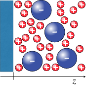
Figure 1: A schematic representation of the asymmetric system composed of particles with unequal sizes and unequal valences in the vicinity of a charged surface.

In the theory of ionic liquids [1] steric effects are of particular importance since the packing of ions can be especially dense [2]. The most common and simplest analytic approach to these effects is via the lattice gas mean-field approximation [3]. This methodology can be furthermore extended to a general local thermodynamic approach for any model of inhomogeneous fluids [4]. In this way one can connect the equation of state for any reference uncharged fluid, not only a lattice gas, with a full description of the same fluid with charged particles on the mean-field electrostatics level, generalizing in this way the Poisson-Boltzmann theory with consistent inclusion of packing effects. This approach is particularly relevant for analysis of dense electric double layers as arise in the context of ionic liquids or dense Coulomb fluids in general [5]. We will use this general local thermodynamics approach in conjunction with two such model equations of state: the asymmetric lattice gas approximation and the asymmetric Carnahan-Starling approximation. The size asymmetry as well as the charge asymmetry, Fig. 1, that this approach allows us to analyse, are fundamentally important for understanding the nature of the electrostatic double layers.

In what follows we will first formulate the local thermodynamics mean-field approach to Coulomb fluids and then apply it to the asymmetric lattice gas, derived within the Flory-Huggins lattice approximation, comparing its results with the asymmetric Carnahan-Starling approximation. As a sideline we also derive several useful general relations valid specifically for the asymmetric lattice gas approximation in the context of electrostatic double layers.

2 General formulation

We proceed by studying the Legendre transform of the free energy density $f(c_{1},c_{2})$ of an isothermal ($T=const$) binary mixture

$$f(c_{1},c_{2})-\mu_{1}c_{1}-\mu_{2}c_{2},$$ (1)

where $c_{1,2}$ are the densities of the two components, and the chemical potentials $\mu_{1,2}$ are defined as

$$\mu_{1,2}=\frac{\partial f(c_{1},c_{2})}{\partial c_{1,2}}.$$ (2)

By the well known thermodynamic relationships [4] the Legendre transform eq. (1) equals

$$f(c_{1},c_{2})-\frac{\partial f(c_{1},c_{2})}{\partial c_{1}}c_{1}-\frac{\partial f(c_{1},c_{2})}{\partial c_{2}}c_{2}=-p(c_{1},c_{2}),$$ (3)

where $p(c_{1},c_{2})$ is the thermodynamic pressure, or the equation of state. For the inhomogeneous case we now invoke the local thermodynamic approximation so that the inhomogeneity is described solely via the coordinate dependence of the densities, but the form of the thermodynamic potential remains the same as in the bulk,

$${\cal F}=\int_{V}\!\!\!d^{3}{\bf r}\left(f(c_{1},c_{2})-\mu_{1}c_{1}-\mu_{2}c_{2}\right)=-\int_{V}\!\!\!d^{3}{\bf r}\leavevmode\nobreak\ p(\mu_{1},\mu_{2}).$$ (4)

In the case of charged particles one needs to consider also the electrostatic energy and its coupling to the density of the particles via the Poisson equation, on top of the reference free energy of uncharged particles. The corresponding thermodynamic potential of the charged binary mixture then assumes the form

$${\cal F}[c_{1},c_{2},{\bf D}]=\int_{V}\!\!\!d^{3}{\bf r}\left(f(c_{1},c_{2})-\mu_{1}c_{1}-\mu_{2}c_{2}\right)+$$

$$+\int_{V}\!\!\!d^{3}{\bf r}\left(\frac{{\bf D}^{2}}{2\varepsilon}-\psi\left(\mbox{\boldmath$\nabla$}\cdot{\bf D}-e(z_{1}c_{1}-z_{2}c_{2})\right)\right),$$ (5)

where ${\bf D}={\bf D}({\bf r})$ is the dielectric displacement field, $\varepsilon=\epsilon\epsilon_{0}$ with $\epsilon$ the relative dielectric permittivity, $z_{1,2}$ are the valencies of the two charged species and $\psi=\psi({\bf r})$ is now the Lagrange multiplier field that ensures the local imposition of Gauss’ law [6]. We can write this expression in an alternative form as

$${\cal F}= \int_{V}\!\!\!d^{3}{\bf r}\left(f(c_{1},c_{2})-(\mu_{1}-ez_{1}\psi)c_{1}-(\mu_{2}+ez_{2}\psi)c_{2}\right)+$$

$$+ \int_{V}\!\!\!d^{3}{\bf r}\left(\frac{{\bf D}^{2}}{2\varepsilon}-\psi\mbox{\boldmath$\nabla$}\cdot{\bf D}\right).$$ (6)

Invoking now the identity eq. (4), discarding the boundary terms and minimizing with respect to $\bf D$, we get the final form of the inhomogeneous thermodynamic potential

$${\cal F}[\psi]=-\!\!\!\int_{V}\!\!\!d^{3}{\bf r}\left({\textstyle\frac{1}{2}}{\varepsilon}(\mbox{\boldmath$\nabla$}\psi)^{2}+p(\mu_{1}-ez_{1}\psi,\mu_{2}+ez_{2}\psi)\right).$$ (7)

In the case of charged boundaries one needs to add a surface term $\oint_{S}\psi D_{n}dS$, where $D_{n}$ is the normal component of the electric displacement field at the surface, to the above equation. While the derivation of eq. (7) proceeded entirely on the mean-field level, it can be extended to the case when the Coulomb interactions are included exactly and the mean potential becomes the fluctuating local potential in a functional integral representation of the partition function [7].

Let us note that the signs of the electrostatic terms in eq. (7) are consistent with the definition of the grand canonical partition function, i.e. $\Omega=-pV$, with $\Omega(\lambda,\beta)=\sum_{N=1}^{\infty}\lambda^{N}Q(N,\beta)/N!$, where $Q(N,\beta)$ is the canonical partition function for $N$ particles. The absolute activity is defined as $\lambda=e^{\beta\mu}$. Since electrostatic interactions enter with a Boltzmann factor, $\lambda=e^{\beta\mu}\longrightarrow e^{\beta\mu\mp ez_{1,2}\psi}$, where $-$ is valid for positive and $+$ for negative ions.

For any equation of state $p(\mu_{1},\mu_{2})$ or indeed any model free energy $f(c_{1},c_{2})$ of the reference uncharged system, one now needs to evaluate the proper chemical potentials of the binary components from eq. (2), make a substitution

$$\mu_{1,2}\longrightarrow\mu_{1,2}\mp ez_{1,2}\psi$$

and finally derive the Euler-Lagrange equation for the local electrostatic potential of the form

$${\varepsilon}\mbox{\boldmath$\nabla$}^{2}\psi-\frac{\partial p(\mu_{1}-ez_{1}\psi,\mu_{2}+ez_{2}\psi)}{\partial\psi}=0,$$ (8)

which generalizes a form derived within a symmetric lattice gas approximation [8]. Invoking furthermore the Gibbs-Duhem relation

$$c_{1,2}=\frac{\partial p}{\partial\mu_{1,2}}$$

we derive the Poisson equation as

$$\frac{\partial p(\mu_{1}-ez_{1}\psi,\mu_{2}+ez_{2}\psi)}{\partial\psi}= -ez_{1}\frac{\partial p}{\partial\mu_{1}}+ez_{2}\frac{\partial p}{\partial\mu_{2}}=$$

$$=-e(z_{1}c_{1}-z_{2}c_{2})=q.$$ (9)

where $q$ is the local charge density. Note that the charge density is a derivative w.r.t. potential of a single function, a simple test of consistency for any proposed theory. Together with eq. (8) this constitutes a generalisation of the Poisson-Boltzmann theory for any model of the fluid expressible via an equation of state in the local thermodynamic approximation. This also generalizes some results previously derived only for the lattice gas.

In the case of a single or two planar surfaces, with a normal in the direction of the $z$-axis, so that $\psi({\bf r})=\psi(z)$, the Poisson-Boltzmann equation possesses a first integral of the form

$${\textstyle\frac{1}{2}}{\varepsilon}\psi^{\prime 2}(z)-p(\mu_{1}-ez_{1}\psi(z),\mu_{2}+ez_{2}\psi(z))=-p_{0}$$ (10)

where $p_{0}$ is an integration constant equal to the osmotic pressure of the ions and determined by the boundary conditions. The disjoining (interaction) pressure for two charged surfaces, $\Pi$, is then obtained by subtracting the bulk contribution from the osmotic pressure $p_{0}$. The first integral of the Euler-Lagrange equation can be used to construct an explicit 1D solution, $\psi=\psi(z)$ by quadrature.

In the limiting case of an ideal gas, with the van’t Hoff equation of state $p(c_{1},c_{2})=k_{B}T(c_{1}+c_{2})$ it is straightforward to see that the above theory reduces exactly to the Poisson-Boltzmann approximation [9]. Furthermore, for the binary, symmetric lattice-gas

$$p(c_{1},c_{2})=-\frac{k_{B}T}{a^{3}}\leavevmode\nobreak\ \log{(1-a^{3}(c_{1}+c_{2}))}$$ (11)

where $a$ is the cell size [10], the above formalism yields the results discussed at length by Kornyshev [3]. From eq. (11) we also see one of the weaknesses of the lattice gas approach, as the pressure diverges only very weakly at close packing. We will compare with a more realistic equation of state later in this paper.

3 Asymmetric lattice gas

We start with the free energy density of mixing for a three component lattice gas system composed of species ”1” at concentration $c_{1}$, itself composed of $N_{1}$ subunits, and species ”2” at concentration $c_{2}$, itself composed of $N_{2}$ subunits, in a solvent of (water) molecules of diameter $a$. It can be expressed rather straightforwardly in terms of the volume fractions $\phi_{1},\phi_{2}$ after realizing that it is equivalent to the problem of polydisperse polymer mixtures on the Flory-Huggins lattice level [11]. For a two component system the free energy of mixing can be derived simply as [12]

$$\frac{f(\phi_{1},\phi_{2})\leavevmode\nobreak\ a^{3}}{k_{B}T}=\frac{\phi_{1}}{N_{1}}\log{\phi_{1}}+\frac{\phi_{2}}{N_{2}}\log{\phi_{2}}+$$

$$+(1-\phi_{1}-\phi_{2})\log{(1-\phi_{1}-\phi_{2})},$$ (12)

where the volume fractions $\phi_{1},\phi_{2}$ are defined as

$$\phi_{1,2}=a^{3}c_{1,2}N_{1,2}=R_{1,2}^{3}c_{1,2},$$ (13)

and $N_{1,2}={(R_{1,2}/a)}^{3}$ measures the relative volumes of species 1 and 2, with radii $R_{1,2}$, compared to the solvent with radius $a$. While the size-symmetric lattice gas has a venerable history (for an excellent review see Ref. [2]) there have been fewer previous attempts to master the lattice gas mixtures in the context of size-asymmetric electrolytes [13, 14, 15, 5, 16] and the simple connection with the entropy of lattice polymers has apparently not been noted before.

The chemical potential is then obtained as

$$\mu_{1,2}=\frac{\partial f(c_{1},c_{2})}{\partial c_{1,2}}=\frac{\partial f(\phi_{1},\phi_{2})}{\partial\phi_{1,2}}a^{3}N_{1,2},$$ (14)

that can be evaluated explicitly yielding

$$\mu_{1,2}=\log{\phi_{1,2}}+1-N_{1,2}\left(\log{(1-\phi_{1}-\phi_{2})+1}\right).$$ (15)

The Legendre transform eq. (1) then yields the osmotic pressure, again as a function of both volume fractions

$$-\frac{p(\phi_{1},\phi_{2})\leavevmode\nobreak\ a^{3}}{k_{B}T}=\log{(1-\phi_{1}-\phi_{2})}+$$

$$+\phi_{1}\left(1-\frac{1}{N_{1}}\right)+\phi_{2}\left(1-\frac{1}{N_{2}}\right).$$ (16)

The form of this result is revealing as it states that the osmotic pressure is basically the lattice gas pressure of a symmetric mixture, corrected by the fact that $N_{1,2}$ subunits of the species ”1” and ”2” do not represent separate degrees of freedom. Obviously, for a symmetric system with $N_{1,2}=1$ this reduces exactly to the lattice gas symmetric binary mixture expression, eq. (11).

Introducing $\tilde{\mu}_{1,2}=\mu_{1,2}+N_{1,2}-1$ we can rewrite eq. (15) as

$$\phi_{1,2}={(1-\phi_{1}-\phi_{2})}^{N_{1,2}}\leavevmode\nobreak\ e^{\tilde{\mu}_{1,2}}$$ (17)

Using this relation we can derive an explicit equation for

$$u=(1-\phi_{1}-\phi_{2})$$ (18)

of the form

$$u\left(1+u^{N_{1}-1}e^{\tilde{\mu}_{1}}+u^{N_{2}-1}e^{\tilde{\mu}_{2}}\right)=1,$$ (19)

that yields $u=u(\tilde{\mu}_{1},\tilde{\mu}_{2};N_{1},N_{2})$. This allows us to finally write the osmotic pressure as a function of the two densities

$$-\frac{p(c_{1},c_{2})\leavevmode\nobreak\ a^{3}}{k_{B}T}=\log{(1-a^{3}(c_{1}N_{1}+c_{2}N_{2}))}+$$

$$+a^{3}c_{1}\left(N_{1}-1\right)+a^{3}c_{2}\left(N_{2}-1\right),$$ (20)

or of the two chemical potentials through $u=u(\tilde{\mu}_{1},\tilde{\mu}_{2};N_{1},N_{2})$ as

$$-\frac{p(\mu_{1},\mu_{2})\leavevmode\nobreak\ a^{3}}{k_{B}T}=\log{u}+$$

$$+u^{N_{1}}e^{\tilde{\mu}_{1}}\left(1-\frac{1}{N_{1}}\right)+u^{N_{2}}e^{\tilde{\mu}_{2}}\left(1-\frac{1}{N_{2}}\right).$$ (21)

In the case of ions of the same size, we can set without any loss of generality, that $N_{1}=N_{2}=1$, so that

$$-\frac{p(\mu_{1},\mu_{2})\leavevmode\nobreak\ a^{3}}{k_{B}T}=\log{u(\tilde{\mu}_{1},\tilde{\mu}_{2})}=-\log{\left(1+e^{\tilde{\mu}_{1}}+e^{\tilde{\mu}_{2}}\right)},$$

a standard expression for the symmetric lattice gas [17].

Above equations present a complete set of relations satisfied by the asymmetric lattice gas, being a mixture of two differently sized ions. The addition of mean-field electrostatic interactions eq (8) then modifies solely the chemical potentials so that

$$p(\mu_{1},\mu_{2})\longrightarrow p(\mu_{1}-ez_{1}\psi,\mu_{2}+ez_{2}\psi)$$ (23)

if the two species are oppositely charged, which we assume. The corresponding Poisson-Boltzmann equation is then obtained from eq. 8 and eq. 9 in the form

$${\varepsilon}\mbox{\boldmath$\nabla$}^{2}\psi\!\!\! = \!\!\!-e\left(z_{1}{\partial_{\mu_{1}}}-z_{2}{\partial_{\mu_{2}}}\right)p(\mu_{1}-ez_{1}\psi,\mu_{2}+ez_{2}\psi)=$$ (24)

$$= -e(\frac{z_{1}}{N_{1}}\phi_{1}(\psi)-\frac{z_{2}}{N_{2}}\phi_{2}(\psi)).$$

where $\phi_{1,2}(\psi)$ are obtained from eq. 17 and 19 with $\tilde{\mu}_{1}\longrightarrow\tilde{\mu}_{1}-ez_{1}\psi,\tilde{\mu}_{2}\longrightarrow\tilde{\mu}_{2}+ez_{2}\psi$.

In complete analogy with the case of polyelectrolytes with added salt [18] it is clear that electroneutrality of the asymmetric lattice gas in the bulk is achieved only if it is held at a non-zero electrostatic potential, $\psi_{0}$, that can be obtained from eq. (24) in an implicit form

$$(N_{1}-N_{2})\log{u(\psi_{0})}=-({\tilde{\mu}_{1}-\tilde{\mu}_{2}})+\log{\frac{N_{1}z_{2}}{N_{2}z_{1}}}.$$ (25)

In what follows we then simply displace the origin of the electrostatic potential by $\psi_{0}$, the Donnan potential, interpreted as the change in electrostatic potential across the bulk reservoir - ionic liquid interface, or equivalently as a Lagrange multiplier for the constraint of global electroneutrality [19].

4 Asymptotic behaviour of the lattice gas model

We now consider the forms of the general equations derived above in the limiting cases of small and large electrostatic potential of the lattice gas model:

4.1 Small potential and screening length

In the limit of $\psi\rightarrow 0$, one can derive

$$p(\mu_{1}+ez_{1}\psi,\mu_{2}-ez_{2}\psi)=p(\mu_{1},\mu_{2})\leavevmode\nobreak\ +$$

$$\qquad-e\left(z_{1}{\partial_{\mu_{1}}}-z_{2}{\partial_{\mu_{2}}}\right)p(\mu_{1},\mu_{2})\psi\leavevmode\nobreak\ +$$

$$\qquad+{\textstyle\frac{1}{2}}e^{2}{\left(z_{1}{\partial_{\mu_{1}}}-z_{2}{\partial_{\mu_{2}}}\right)^{2}}p(\mu_{1},\mu_{2})\leavevmode\nobreak\ \psi^{2}+{\cal O}(\psi^{3})$$ (26)

where we took into account eq. (9). Just as in the full non-linear case, see above, the term linear in $\psi$ is connected with the displaced electrostatic potential, eq. (25). The linearized form of $\psi_{0}$ is then obtained approximately as

$$\psi_{0}=\frac{e\left(z_{1}{\partial_{\mu_{1}}}-z_{2}{\partial_{\mu_{2}}}\right)p(\mu_{1},\mu_{2})}{e^{2}{\left(z_{1}{\partial_{\mu_{1}}}-z_{2}{\partial_{\mu_{2}}}\right)^{2}}p(\mu_{1},\mu_{2})}.$$ (27)

Obviously the expansion of the pressure for small values of the electrostatic potential is then quadratic in the difference $\psi-\psi_{0}$.

Furthermore, the Hessian of the pressure $p(\mu_{1},\mu_{2})$ is positive definite, i.e.

$$\frac{e^{2}}{\varepsilon}\left(z_{1}^{2}\frac{\partial^{2}p}{\partial\mu_{1}^{2}}-2z_{1}z_{2}\frac{\partial^{2}p}{\partial\mu_{1}\mu_{2}}+z_{2}^{2}\frac{\partial^{2}p}{\partial\mu_{2}^{2}}\right)=\kappa^{2}>0,$$ (28)

while from eq. (7) it follows that $\kappa$ is nothing but the inverse Debye length expressed through the second derivatives of the pressure with respect to the chemical potentials of both charged species. Since the curvature tensor of the Legendre transform is the inverse of the curvature tensor of the function itself [20], we can write

$$\sum_{m}\frac{\partial^{2}p(\mu_{1},\mu_{2})}{\partial\mu_{i}\partial\mu_{m}}\frac{\partial^{2}f(c_{1},c_{2})}{\partial c_{m}\partial c_{k}}=\delta_{ik}$$ (29)

where all the matrices are $2\times 2$. From here it follows rather straightforwardly that

$$\kappa^{2}= \frac{e^{2}}{\varepsilon}\frac{z_{2}^{2}\frac{\partial^{2}f}{\partial c_{1}^{2}}+2z_{1}z_{2}\frac{\partial^{2}f}{\partial c_{1}\partial c_{1}}+z_{1}^{2}\frac{\partial^{2}f}{\partial c_{2}^{2}}}{\frac{\partial^{2}f}{\partial c_{1}^{2}}\frac{\partial^{2}f}{\partial c_{2}^{2}}-{\left(\frac{\partial^{2}f}{\partial c_{1}\partial c_{2}}\right)}^{2}}$$

$$= 4\pi\ell_{B}N_{1}N_{2}\frac{u(z_{1}^{2}c_{1}+z_{2}^{2}c_{2})+a^{3}c_{1}c_{2}{({z_{1}}{N_{2}}+{z_{2}}{N_{1}})}^{2}}{(1+(N_{1}-1)a^{3}N_{1}c_{1}+(N_{2}-1)a^{3}N_{2}c_{2})},$$

where we introduced the Bjerrum length $\ell_{B}=e^{2}/(4\pi\varepsilon k_{B}T)$. In general the Debye length is therefore not a linear function of the concentrations. For the symmetric lattice gas, $N_{1}=N_{2}=1$, and taking into account the definition eq. 18, the above result reduces to $\kappa^{2}=4\pi\ell_{B}\left(z_{1}^{2}c_{1}+z_{2}^{2}c_{2}-a^{3}{(z_{1}c_{1}-z_{2}c_{2})}^{2}\right)$, which for bulk electroneutrality reduces further to the standard Debye expression[17].

4.2 Large potential and close packing

The limits for $\psi\rightarrow\pm\infty$ of a lattice gas can be derived as

$$u=\left\{\begin{array}[]{ll}e^{-(\tilde{\mu}_{1}+ez_{1}\psi)/N_{1}}&\psi\rightarrow+\infty\\ e^{-(\tilde{\mu}_{2}-ez_{2}\psi)/N_{2}}&\psi\rightarrow-\infty\end{array}\right.$$ (31)

implying

$$\phi_{1,2}(\psi\rightarrow\infty)=\left\{\begin{array}[]{l}1\\ e^{-(\tilde{\mu}_{1}+ez_{1}\psi)N_{2}/N_{1}+(\tilde{\mu}_{2}-ez_{2}\psi)}\end{array}\right..$$ (32)

and

$$\phi_{1,2}(\psi\rightarrow-\infty)=\left\{\begin{array}[]{l}e^{-(\tilde{\mu}_{2}-ez_{2}\psi)N_{1}/N_{2}+(\tilde{\mu}_{1}-ez_{1}\psi)}\\ 1\end{array}\right..$$ (33)

where the upper formula is for ”1” and the lower for ”2”. Thus

$$-\frac{p(\psi\rightarrow\infty)\leavevmode\nobreak\ a^{3}}{k_{B}T}=-(\tilde{\mu}_{1}+ez_{1}\psi)/N_{1}+$$

$$+\left(1-\frac{1}{N_{1}}\right)+e^{-(\tilde{\mu}_{1}+ez_{1}\psi)N_{2}/N_{1}}e^{(\tilde{\mu}_{2}-ez_{2}\psi)}\left(1-\frac{1}{N_{2}}\right)$$

and

$$-\frac{p(\psi\rightarrow-\infty)\leavevmode\nobreak\ a^{3}}{k_{B}T}=-(\tilde{\mu}_{2}-ez_{2}\psi)/N_{2}+$$

$$+e^{-(\tilde{\mu}_{2}-ez_{2}\psi)N_{1}/N_{2}}e^{(\tilde{\mu}_{1}+ez_{1}\psi)}\left(1-\frac{1}{N_{1}}\right)+\left(1-\frac{1}{N_{2}}\right)$$

The most striking feature of these limits is the linear behaviour of $p(\psi)$ for large positive or negative potentials, which gives rise to a V-like curve for symmetric particles. This linear behaviour is linked to the saturation of close packing of the lattice particles against a high potential surface. For particle of unequal size the two branches of $p(\psi)$ have different slopes.

5 A dense two component lattice gas

For some cases in the theory of ionic liquids one can assume dense packing, without any intervening solvent, so that $\phi_{1}+\phi_{2}=1$. The corresponding free energy can then be cast into a simplified form

$$\frac{f(\phi_{1},\phi_{2}=1-\phi_{1})\leavevmode\nobreak\ N_{2}a^{3}}{k_{B}T}=\frac{\phi_{1}}{M}\log{\phi_{1}}+{\phi_{2}}\log{\phi_{2}}.$$

where $M=N_{1}/N_{2}$ is the effective size of the species ”1” compared to species ”2”. This implies furthermore that

$$\frac{\partial f}{\partial\phi_{1}}+\frac{\partial f}{\partial\phi_{2}}=0\longrightarrow\mu_{1}+M\mu_{2}=0.$$ (37)

The equation analogous to eq. (19) then assumes the form

$$\phi_{1}={(1-\phi_{1})}^{M}e^{\mu_{1}-1+M}$$ (38)

and the Legendre transform of the free energy density follows as

$$\!\!\!-\frac{p(\phi_{1},\phi_{2}=1-\phi_{1})\leavevmode\nobreak\ N_{2}a^{3}}{k_{B}T}=\log{\phi_{2}}+\phi_{1}\left(1-\frac{1}{M}\right).$$

The Poisson-Boltzmann equation is then cast into a simplified form

$$\varepsilon\nabla^{2}\psi= -e\left(z_{1}{\partial_{\mu_{1}}}-z_{2}{\partial_{\mu_{2}}}\right)p(\mu_{1}-ez_{1}\psi,\mu_{2}+ez_{2}\psi)=$$

$$=\frac{1}{N_{1}}\left((z_{1}+Mz_{2})\phi_{1}-Mz_{2}\right),$$ (40)

and the charge density is constrained to be between $-\frac{z_{2}}{N_{2}}$ and $\frac{z_{1}}{N_{1}}$.

6 Asymmetric Carnahan-Starling approximation

In order to show the interest and generality of our local thermodynamic approach we will now apply it in the case of the Carnahan - Sterling approximation for asymmetric binary hard sphere mixtures [21]. For a bulk, uncharged hard sphere fluid the Carnahan-Starling  approximation is ”almost exact”.

The excess pressure in the Carnahan-Starling  approximation derived via the ”virial equation” is then equal to

$$\frac{p_{exc}(c_{1},c_{2})}{ck_{B}T}=\frac{(1+\xi+\xi^{2})-3\xi(y_{1}+\xi y_{2})-3\xi^{3}y_{3}}{{(1-\xi)}^{3}}$$ (41)

where $c_{1,2}$ are the densities of the two components and

$$\xi_{1,2}=\frac{4\pi}{3}R_{1,2}^{3}c_{1,2}\qquad{\rm and}\qquad\xi=\xi_{1}+\xi_{2},$$ (42)

where $R_{1,2}$ are the hard sphere radii of the two species. Furthermore

$$y_{1}= \Delta_{12}\frac{R_{1}+R_{2}}{\sqrt{R_{1}R_{2}}}\qquad y_{2}=\Delta_{12}\frac{\xi_{1}R_{2}+\xi_{2}R_{1}}{\sqrt{R_{1}R_{2}}\xi}$$

$$y_{3}= {\left({\left(\frac{\xi_{1}}{\xi}\right)}^{2/3}+{\left(\frac{\xi_{2}}{\xi}\right)}^{2/3}\right)}^{3}$$ (43)

with

$$\Delta_{12}=\frac{\sqrt{\xi_{1}\xi_{2}}}{\xi}\frac{{(R_{1}-R_{2})}^{2}}{R_{1}R_{2}}.$$ (44)

The excess free energy then follows as

$$\frac{f_{exc}(c_{1},c_{2})}{ck_{B}T}= -{\textstyle\frac{3}{2}}\left(1-y_{1}+y_{2}+y_{3}\right)+$$

$$+\frac{3y_{2}+2y_{3}}{1-\xi}+{\textstyle\frac{3}{2}}\frac{1-y_{1}-y_{2}-{\textstyle\frac{1}{3}}y_{3}}{{(1-\xi)}^{2}}+$$

$$+(y_{3}-1)\log{(1-\xi)},$$ (45)

It is now straightforward to obtain the chemical potentials from the free energy as $\mu_{1,2}=\mu_{1,2}(c_{1},c_{2})$, invert them and then obtain the pressure equation as $p=p(\mu_{1},\mu_{2})$.

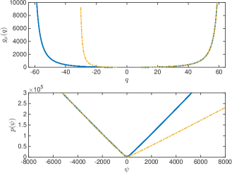
Figure 2: Top: the function $g_{\mu}(q)$ for a Carnahan-Starling fluid. It is an effective potential at imposed local charge density. The divergences correspond to the close packing of the fluid. Blue: symmetric particle volumes. Gold: asymmetric fluid with larger negative particles. This function is important in dual convex formulations of the Poisson-Boltzmann equation, see eq. (62). Bottom: the function $p(\psi)$ for the same two sets of fluid parameters. Blue: Seen from afar the function displays a characteristic V-like behaviour for symmetric particles. The larger particles, gold, give a smaller slope in the pressure function. The central part of the figure for symmetric particles is examined more closely in figure 3

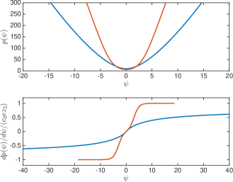
Figure 3: Comparison of symmetric Carnahan-Starling and lattice gas forms near $\psi=0$. Top $p(\psi)$, bottom charge density $-q(\psi)=dp/d\psi$. Carnahan-Starling in blue, converges very slowly to the slope final value, (see figure. 4), and is much broader at minimum compared to the lattice gas curve (red). Physical parameters are such that the blue and red curves have asymptotically the close packing charge density; the chemical potentials have been tuned to give the same Debye length in the bulk (corresponding to the same curvature at the origin in the curve for $p$). Despite this double matching the curves are very different in functional form. The curve $q(\psi)$ for the Carnahan-Starling fluid converges extraordinarily slowly compared with the lattice gas approximation.

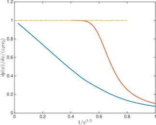
Figure 4: Study of the evolution of $-q=dp(\psi)/d\psi$ in variables adapted to the Carnahan-Starling fluid, (blue). The large field behaviour is linear in $1/\psi^{1/3}$, demonstrating the correctness of arguments leading to eq. (48). Same data as fig. 3 for large positive potentials. The lattice gas model (red) gives much more rapid cross-over to saturation at large potentials. Horizontal line is to guide the eye and corresponds to the close packing charge density.

7 Asymptotic behaviour for the Carnahan-Starling free energy density

In the limit of large potentials $\psi$, as occurs near an electrode, the second, wrongly charged, component of the fluid is excluded and the dominant physics is the packing of a single component system under the constraints coming from the electrostatic interactions. In this limit of $\xi\longrightarrow 1$ we can substitute $y_{1,2}=0$ and $y_{3}=1$. The most important divergence in this limit thus stems from the denominator in eq. (45).

The free energy density of a Carnahan-Starling liquid near close packing has a singularity of the form

$$f(c)=\frac{c_{0}k_{B}T}{{(1-c/c_{0})}^{2}}$$ (46)

$c_{0}$ is the close packing volume fraction of the component dominating near the electrode. With this assumption we can take the Legendre transform of the most singular, diverging part of the free energy to find the large potential limit of $p(\psi)$. For large positive $\psi$ (assuming that $ez_{2}\psi\gg\mu$) this limit turns out to be

$$p(\psi)=z_{2}ec_{0}\psi-\frac{3}{2}{(2c_{0}k_{B}T)}^{1/3}{(z_{2}ec_{0}\psi)}^{2/3}$$ (47)

where we have used the fact that negative ions of valence $z_{2}$ dominate.

In the high packing limit $p(\psi)$ is therefore linear in the potential, and is given by the spatial charge density at close packing exactly like for the lattice gas. However unlike the lattice gas the approach to the high field limit is very slow

$$-q(\psi)=z_{2}ec_{0}-\Big{(\frac{2c_{0}k_{B}T}{\psi}\Big{)}}^{1/3}{(z_{2}ec_{0})}^{2/3}$$ (48)

The spatial charge density is negative for large positive potentials. The correctness of this law is demonstrated in figure 4 which plots $(1/c_{0}z_{2}e)dp/d\psi$ as a function of $\psi^{-1/3}$. The curve linearly extrapolates to unity for large $\psi$. There is a very clear contrast with the case of the lattice gas model where the cross-over to close packing occurs for much smaller values of the potential.

7.1 Solution for the high field Carnahan-Starling limit

The solution for the generalized Poisson-Boltzmann equation in the high field limit can be found from the solution of the integral problem

$$\int\!\!{d\psi}{\left(ec_{0}z_{2}\psi-\beta{(ec_{0}z_{2}\psi)}^{2/3}+p_{0}\right)}^{-1/2}=\sqrt{\frac{2}{\varepsilon}}\int\!\!dz$$ (49)

with $\beta=3{(2c_{0}k_{B}T)}^{1/3}/2$; we neglect $\mu$ compared to $z_{2}e\psi$. This integral can be transformed by substituting ${(ec_{0}z_{2}\psi)}^{1/3}=y$, giving

$$3\int\!\frac{dy\leavevmode\nobreak\ y^{2}}{{(y^{3}-\beta y^{2}+p_{0})}^{1/2}}=\sqrt{\frac{2e^{2}c_{0}^{2}z_{2}^{2}}{\varepsilon}}\int\!dz,$$ (50)

a form which can be solved by using elliptic functions. If we make the further approximation that $p_{0}$ is small we can find much simpler expressions:

$$z(\psi)-z_{0}= \frac{\sqrt{2\epsilon}}{ec_{0}z_{2}}[{({(z_{2}ec_{0}\psi)}^{1/3}-\beta)}^{3/2}+$$

$$3 \beta{({(z_{2}ec_{0}\psi)}^{1/3}-\beta)}^{1/2}]$$ (51)

Here, $z(\psi)$ gives the distance from a plate which corresponds to a potential $\psi$. It is obviously the inverse function of $\psi(z)$. We perform a “numerically exact” calculation of the curve $\psi(z)$ in fig. (5) in the inset, where we place a positve electrode at $z=0$. The main figure of fig. (5) contains three curves: The blue curve explodes part of the inset and is overlayed with a red curve corresponding to eq. (51). On this scale the results are indistinguishable. The green curve is evaluated by assuming perfect packing of the fluid against the electrode. Eq. (51) is clearly a much better description of the high electrostatic potential physics.

Eq. (51) can also be combined with eq. (48) to find $z(q)$ and thus the evolution of the spatial charge density with distance from an electrode as well as the variation of the local charge density with the potential.

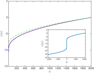
Figure 5: Carnahan-Starling fluid. Blue: exact numerical calculation of the function $z(\psi)$. The full curve is given in the inset. The high field limit studied in the main panel. Red: approximation valid for large fields from eq. (51). Green profile calculated from assuming perfect packing of the fluid against electrode. Blue and red curves almost perfectly correspond, with no extra fitting parameters.

8 Differential Capacitance

Together with the boundary condition $D_{n}=\sigma$, where $\sigma$ is the surface charge density one can derive the equivalent of the Grahame equation in the form

$$\frac{\sigma^{2}}{{2\varepsilon}}-p(\mu_{1}-ez_{1}\psi_{0},\mu_{2}+ez_{2}\psi_{0})=-p_{0},$$ (52)

assuming that the bounding surface is located at $z=0$, i.e. $\psi_{0}=\psi(z=0)$. From the Grahame equation one can next derive the differential capacitance $\cal C$ as

$${\cal C}(\psi_{0})=\frac{\partial\sigma(\psi_{0})}{\partial\psi_{0}}= \frac{\varepsilon e}{\sigma(\psi_{0})}\left(-z_{1}\frac{\partial p}{\partial\mu_{1}}+z_{2}\frac{\partial p}{\partial\mu_{2}}\right)=$$

$$= \frac{-\varepsilon e(z_{1}c_{1}-z_{2}c_{2})}{\pm\sqrt{2\varepsilon(p-p_{0})}},$$ (53)

with $\pm$ depending on the sign of the surface charge. Taking into account the definition of the Bjerrum length, $\ell_{B}$

$${\cal C}^{2}(\psi_{0})=2\pi{k_{B}T}\ell_{B}\frac{(z_{1}c_{1}(\psi_{0})-z_{2}c_{2}(\psi_{0}))^{2}}{{p(\psi_{0})-p_{0}}}.$$ (54)

Invoking the Poisson-Boltzmann equation for this case, an alternative form of the differential capacitance is

$${\cal C}(\psi_{0})= {\varepsilon}\left(\log{\psi_{0}^{\prime}}\right)^{\prime}=$$

$$= \sqrt{{2}{\varepsilon}}\frac{\partial}{\partial\psi_{0}}\sqrt{p(\mu_{1}-ez_{1}\psi_{0},\mu_{2}+ez_{2}\psi_{0})-p_{0}},$$ (55)

the form that we use in our numerical work. It is interesting to note that even if we shift the minimum of the curve $p(\psi)$ to occur at $\psi=0$ this does not imply that $\psi=0$ is also a stationary value of the differential capacitance. This is clearly visible in the curves of fig. (6) where in denser fluids the maximum of the curves is shifted to positive potentials. We mark the position of the minimum in $p(\psi)$ by a slight break in the solid lines. This displacement of the maximum of the capacitance from the minimum of $p$ is trivially understood if one assumes that the expansion of $p(\psi)$ includes a term in $\psi^{3}$. We see that the qualitative behaviour of the curves generated for the lattice model, as well as the Carnahan-Starling fluid are rather similar.

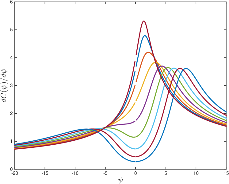
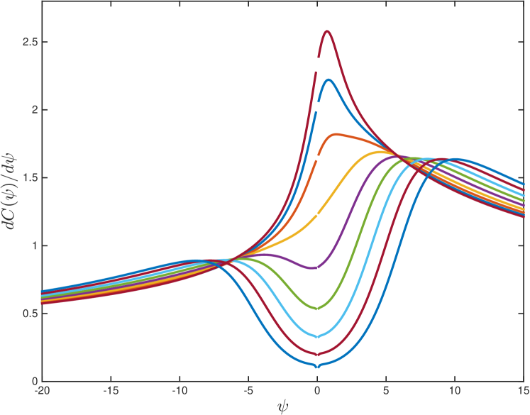
Figure 6: Top: calculation of the differential capacitance for a volume asymmetric lattice fluid. Bottom: volume asymmetric Carnahan-Starling fluid. From eq. (55). Each curve is for a different value of the chemical potential, $\mu$. Strongly negative chemical potentials give a minimum in the curves near $\psi=0$, together with two asymmetric maxima. As the chemical potential increases the curves develop a peak near (but not at) $\psi=0$. The chemical potential has been shifted such that the minimum of $p(\psi)$ is at $\psi=0$. In both cases the positively charged component has a volume $1.5^{3}$ larger than the negative component.

9 Conclusions

By using general arguments based upon local thermodynamics, we generalized the Poisson-Boltzmann mean-field theory of Coulomb fluids to the case where the reference, uncharged fluid need not be ideal. We formulated the general theory in the particular cases of an asymmetric lattice gas and an asymmetric Carnahan-Starling liquid that describe steric effects at various levels of approximations and are particularly relevant for analysis of dense electric double layers as arise in the context of ionic liquids or dense Coulomb fluids. Use of properties of Legendre transforms allows us to efficiently translate between forms of the free energy; this includes a standard formulation in terms of the electrostatic potential, and a dual formulation (see appendix) in terms of the electric displacement field.

We analyzed in detail the size and charge asymmetry and their respective effects on the salient properties of electric double layers. As part of our analysis we also formulated an exact thermodynamic description of an asymmetric lattice gas, derived within the Flory-Huggins lattice approximation. This allows the lattice gas approximation, which in its symmetric form already serves as the most popular description of the steric effects in the context of the Poisson-Boltzmann theory [2], to be further extended to the case of ubiquitous size-asymmetric dense ionic mixtures. It is probably in this latter case that it will prove to be most useful specifically in the context of ionic liquids [1].

For the Carnahan-Starling fluid we have found an asymptotic form that gives a rather simple analytic relation between potential and distance, eq. (51), as well as the relation between potential and local charge density eq. (48). It is clear that the description of charged fluids as lattice gases or as charged hard spheres gives very different phenomenology in high field regions. The lattice gas crosses over very rapidly to a close packed system, whereas much higher fields are needed to compress the hard sphere system, leading to very slow cross-overs in $1/\psi^{1/3}$ in physical properties such as charge density.

10 Appendices

10.1 Numerical methods

We wrote numerical codes to study the double Legendre transformed free energy

$$f(c_{1},c_{2})-\mu(c_{1}+c_{2})-\tilde{\psi}(z_{1}c_{1}-z_{2}c_{2})$$ (56)

where $\tilde{\psi}=-\psi$. We do this by working with the effective coordinates

$$n= (c_{1}+c_{2})$$

$$q= (z_{1}c_{1}-z_{2}c_{2})$$ (57)

So that we are interested in stationary points of the function.

$$\tilde{f}(n,q)-\mu n-\tilde{\psi}q$$ (58)

where we have expressed the free energy as a function of the two independent coordinates, $n$ the number density and $q$ the charge density.

We proceed by constructing an intermediate function $g_{\mu}(q)$ by numerical minimisation of eq (58), with fixed $\mu$ and $q$, with $\tilde{\psi}=0$. The function $g_{\mu}(q)$ is then passed to the Chebfun library [22, 23] which evaluates $g_{\mu}(q)$ for different specific values of $q$ and builds a Chebyshev approximant accurate to a relative accuracy of $10^{-15}$. From this function we build the Legendre transform from $q$ to $\tilde{\psi}$ by standard operations on $g_{\mu}$ [20].

$$g_{\mu}(q)\rightarrow g_{\mu}^{\prime}(q)\rightarrow{(g_{\mu}^{\prime})}^{-1}(\tilde{\psi})\rightarrow\int^{\tilde{\psi}}{(g_{\mu}^{\prime})}^{-1}(\psi^{\prime})d\psi^{\prime}$$ (59)

These steps are all performed by manipulation of the Chebyshev series, while maintaining close to machine precision in the evaluations. The result is an approximant to $p(\tilde{\psi})$. The last step is to transform back to $p(\psi)$ which requires a flip in sign of the potential axes.

The functions $p(\psi)$ and $g_{\mu}(q)$ encode complementary information on the physical system. We can find the equilibrium charge density at a given potential from the relation

$$q(\psi)=-\frac{dp}{d\psi}$$ (60)

we find the potential at imposed charge density from

$$\psi(q)=-\frac{dg_{\mu}}{dq}$$ (61)

The non-standard signs in these relations come from the difference between $\psi$ and $\tilde{\psi}$.

The question finally arrises as to how to use the numerically determined curves for $p(\psi)$ in other external codes. Inspiration comes from the Carnahan-Starling approximation for the pressure which is a ratio of polynomials in the density. Such a general form is an example of a Padé approximant that yields a high precision representation of the function $p(\psi)$ with an approximation as a ratio of two cubic polynomials that yields a rather good fit. Use of two quartics gives results which are visually perfect. Thus the present functional forms can be easily exported (this is even part of the chebfun library) to simple, fast approximations that can be used in other simulation codes.

Clearly these methods are completely general can be applied to even more elaborate equations of state, extrapolated from the best virial expansions [24].

10.2 Convex formulation for Poisson-Boltzmann free energies

As an alternative to writing the Poisson-Boltzmann functional in terms of the potential $\psi$ with the help of the function $p(\psi)$ we can generate an equivalent convex formulation using the displacement field $\bf D$. As shown in [25, 26] this exact transformation requires the Legendre transfrom of the function $p(\psi)$. However, we have already evaluated this object, it is just $g_{\mu}(q)$, eq. (59). We can thus at once conclude that the general convex Poisson-Boltzmann function equivalent to those discussed above is

$$f({\bf D})=\frac{{\bf D}^{2}}{2\varepsilon}+g_{\mu}({\rm div\,}{\bf D}-\rho_{e})$$ (62)

with $\rho_{e}$ the external, imposed charged density. This form can be particularly interesting for the numerical work when coupling to other conformational degrees of freedom such as polymer chains or biomolecules. While we do not have analytic expression for $g_{\mu}$ for the Carnahan-Starling fluid it is again easy to generate the curve as a Chebyshev polynomial and export them to an accurate and efficient form for use in other codes.

11 Acknowledgment

A.C.M. is partially financed by the ANR grant FSCF. R.P. thanks the hospitality of L’École supérieure de physique et de chimie industrielles de la ville de Paris (ESPCI ParisTech) during his stay as a visiting Joliot chair professor and acknowledges partial support of the Slovene research agency (ARRS) through grant P1-0055.

References

- [1] \NameFedorov M. V. Kornyshev A. A. \REVIEWChem. Rev.11420142978.
- [2] \NameBazant M. Z., Kilic M. S., Storey D. Ajdari A. \REVIEWAdvances in Colloid and Interface Science152200948.
- [3] \NameKornyshev A. A. \REVIEWJ. Phys. Chem. B11120075545.
- [4] \NameRowlinson J. Widom B. \BookMolecular theory of capilarity (Dover, Mineola, NY) 2002.
- [5] \NameBiesheuvel P. van Soestbergen M. \REVIEWJournal of Colloid and Interface Science3162007490.
- [6] \NameMaggs A. C. \REVIEWThe Journal of Chemical Physics11720021975.
- [7] \NameWiegel F. W. \BookIntroduction to path-integral methods in physics and polymer science (World Scientific, Singapore) 1986.
- [8] \NameTrizac E. Raimbault J. \REVIEWPhys. Rev. E6019996530.
- [9] \NameBen-Yaakov D., Andelman D., Podgornik R. Harries D. \REVIEWCurrent Opinion in Colloid and Interface Science162011542.
- [10] \NameBen-Yaakov D., Andelman D., Harries D. Podgornik R. \REVIEWJ Phys: Condens Matter212009424106.
- [11] \NameTeraoka I. \BookPolymer Solutions: An Introduction to Physical Properties (Wiley Interscience, John Wiley and Sons Inc., New York) 2002.
- [12] \NamePodgornik R., Hopkins J. C., Parsegian V. A. Muthukumar M. \REVIEWMacromolecules4520128921.
- [13] \NameEigen M. Wicke E. \REVIEWJ Phys Chem.581954702.
- [14] \NameChu V. B., Bai Y., Lipfert J., Herschlag D. Doniach S. \REVIEWBiophysical Journal9320073202.
- [15] \NameZhou S., Wang Z. Li B. \REVIEWPhys. Rev. E842011021901.
- [16] \NamePopović M. Šiber A. \REVIEWPhys. Rev. E882013022302.
- [17] \NameBorukhov I., Andelman D. Orland H. \REVIEWElectrochimica Acta462000221.
- [18] \NameRamanathan G. Woodbury C. \REVIEWJ. Chem. Phys.8219851482.
- [19] \NameDenton A. R. \BookCoarse-grained modeling of charged colloidal suspensions: From poisson-boltzmann theory to effective interactions in \BookElectrostatics of soft and disordered matter, edited by \NameDean D. S., Dobnikar J., Naji A. Podgornik R. (Pan Stanford, Singapore) 2014.
- [20] \NameZia R., , Redish E. F. McKay S. R. \REVIEWAm. J. Phys.772009614.
- [21] \NameMansoori G., Carnahan N., Starling K. Leland T. \REVIEWJournal of Chemical Physics5419711523.
- [22] \NameTrefethen L. N. \REVIEWMathematics in Computer Science120079.
-
[23]
\NameDriscoll T. A., Hale N. Trefethen L. N. \BookChebfun Guide
(Pafnuty Publications) 2014.
http://www.chebfun.org/docs/guide/ - [24] \NameBannerman M. N., Lue L. Woodcock L. V. \REVIEWThe Journal of Chemical Physics1322010.
- [25] \NameMaggs A. C. \REVIEWEPL (Europhysics Letters)98201216012.
- [26] \NamePujos J. S. Maggs A. C. \BookLegendre transforms for electrostatic energies in \BookElectrostatics of soft and disordered matter, edited by \NameDean D. S., Dobnikar J., Naji A. Podgornik R. (Pan Stanford, Singapore) 2014.