A simple non-chaotic map generating subdiffusive, diffusive and superdiffusive dynamics

Abstract

Analytically tractable dynamical systems exhibiting a whole range of normal and anomalous deterministic diffusion are rare. Here we introduce a simple non-chaotic model in terms of an interval exchange transformation suitably lifted onto the whole real line which preserves distances except at a countable set of points. This property, which leads to vanishing Lyapunov exponents, is designed to mimic diffusion in non-chaotic polygonal billiards that give rise to normal and anomalous diffusion in a fully deterministic setting. As these billiards are typically too complicated to be analyzed from first principles, simplified models are needed to identify the minimal ingredients generating the different transport regimes. For our model, which we call the slicer map, we calculate all its moments in position analytically under variation of a single control parameter. We show that the slicer map exhibits a transition from subdiffusion over normal diffusion to superdiffusion under parameter variation. Our results may help to understand the delicate parameter dependence of the type of diffusion generated by polygonal billiards. We argue that in different parameter regions the transport properties of our simple model match to different classes of known stochastic processes. This may shed light on difficulties to match diffusion in polygonal billiards to a single anomalous stochastic process.

Consider equations of motion that generate dispersion of an ensemble of particles as the dynamics evolves in time. A fundamental challenge is to develop a theory for predicting the diffusive properties of such a system starting from first principles, that is, by analyzing the microscopic deterministic dynamics. Here we introduce a seemingly trivial toy model that, analogously to polygonal billiards, exhibits dispersion but is not chaotic in terms of exponential sensitivity with respect to initial conditions. We show that our simple map model generates a surprisingly non-trivial spectrum of different diffusive properties under parameter variation.

I Introduction

How macroscopic transport emerges from microscopic equations of motion is a key topic in dynamical system theory and nonequilibrium statistical physics Do99 ; Gasp ; Kla06 ; RoMM07 ; CFLV08 ; BPRV08 ; JR10 . While microscopic chaos, characterized by positive Lyapunov exponents, typically leads to Brownian motion-like dynamics by reproducing conventional statistical physical transport laws, for weakly chaotic dynamical systems where the largest Lyapunov exponent is zero the situation becomes much more complicated Zas02 ; Kla06 ; KRS08 . Such non-trivial dynamics is relevant for many topical applications like, for example, nanoporous transport JBS03 ; IRP ; JeRo06 ; JBR08 ; Sokolov . In the former case the mean square displacement (MSD) of an ensemble of particles grows linearly in the long time limit, $\langle x^{2}\rangle\sim t^{\gamma}$ with $\gamma=1$ defining normal diffusion. In the latter case one typically finds anomalous diffusion with $\gamma\neq 1$, where for $\gamma<1$ one speaks of subdiffusion, for $\gamma>1$ of superdiffusion MeKl00 ; Zas02 ; KRS08 ; Sokolov .

To our knowledge only a few deterministic dynamical systems are known exhibiting all three regimes of subdiffusion, normal diffusion and superdiffusion under parameter variation. Examples of one-dimensional maps are a Pomeau-Manneville like model where anomalous diffusion originates from an interplay between different marginally unstable fixed points ZuKl95 . The climbing sine map displays exactly three different diffusive regimes with $\gamma=0,1,2$ corresponding to periodic windows and chaotic regions connected to period doubling bifurcations and crises KoKl02 ; KoKl03 . For the two-dimensional standard map numerical evidence exists for a transition from sub- to superdiffusion generated by a mixed phase space ThaRo14 . Least understood is diffusion in two-dimensional polygonal billiards Zas02 ; LWH02 ; LWWZ05 ; Kla06 ; Dett14 ; JeRo06 ; JBR08 , see Fig. 1 for an example. By definition these systems exhibit linear dispersion of nearby trajectories with zero Lyapunov exponents for typical initial conditions, hence non-chaotic behavior. However, they nevertheless generate highly non-trivial dynamics due to complicated topologies yielding pseudohyperbolic fixed points and pseudointegrability. For this reason they are sometimes called pseudochaotic Zas02 ; Kla06 . A line of numerical work on periodic polygonal billiard channels revealed sub-, super- and normal diffusion depending on parameter variation ArGuRe00 ; ARV03 ; SchSt06 ; JeRo06 ; SaLa06 ; JBR08 . Rigorous analytical results are so far only available for periodic wind-tree models supporting an extremely delicate dependence of diffusive properties on variation of control parameters HaWe80 ; DHL11pp . For the mathematical derivations it has been exploited that polygonal billiards can often be reduced to interval exchange transformations (IETs), see also HaMc90 ; Gut96 ; ZaEd01 . These are one-dimensional maps generalising circle rotations which cut the original interval into several subintervals by permuting them non-chaotically. Both polygonal billiards and IETs are known to exhibit hihgly non-trivial ergodic properties, and in general there does not seem to exist any theory to understand the complicated diffusive dynamics of such systems from first principles. Random non-overlapping wind-tree models and related maps, on the other hand, enjoy a kind of stochasticity which appears analogous to the dynamically generated randomness of chaotic systems, leading to sufficiently rapid decay of correlations and good statistical properties. Consequently, these models have been found to yield normal diffusion that is indistinguishable from Brownian motion DC00 ; CFVN02 . In contrast, periodic polygonal billiards have very long lasting dynamical correlations and poor statistical properties, which are associated with very sensitive dependence of their transport properties on the details of their geometry JeRo06 .

These difficulties to understand diffusion in polygonal billiards on the basis of dynamical systems theory are paralleled by difficulties in attempts to approximate their diffusive properties by stochastic theory: There still appears to be a controversy in the literature of whether continuous time random walk theory and Lévy walks, fractional Fokker-Planck equations or scaling arguments should be applied to undestand their anomalous diffusive properties, with different approaches yielding different results for the above exponent $\gamma$ of the MSD Zas02 ; DKU03 ; LWWZ05 ; Kla06 . While all these theories are based on dynamics generated from temporal randomness, spatial randomness leads yet to another important class of stochastic models, called random walks in random environments, which yields related types of anomalous diffusion: An important example in one dimension is the Lévy Lorentz gas where the scatterers are randomly distributed according to a Lévy-stable probability distribution of the scatterer positions. This model has been studied both numerically and analytically revealing a highly non-trivial superdiffusive dynamics that depends in an intricate way on initial conditions and the type of averaging BF99 ; BFK00 ; BCV10 . This work is related to experiments on Lévy glasses where similar behavior has been observed BBW08 .

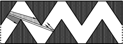
Figure 1: Example of a polygonal billiard channel in which single point particles scatter elastically with sawtooth walls LWH02 ; LWWZ05 ; Kla06 ; JeRo06 . Shown is how a beam of particles is split by the corners of the billiard while propagating.

Figure 2: Space-time plot illustrating the action of the one-dimensional slicer map $S_{\alpha}$ for $\alpha=1/3$ defined by Eqs. (1,2), where $m$ (horizontal axis) denotes space and $n$ (vertical axis) time: Shown is the diffusive spreading of points that at $n=0$ are uniformly distributed on the unit interval centered around $m=0$. As the map is one-dimensional the columns are only a guide to the eye. This map is designed to mimic the mechanism of beam-splitting in polygonal billiards depicted in Fig. 1.

Motivated by the problem of understanding diffusion in polygonal billiards, in this paper we propose a seemingly trivial non-chaotic map by which we attempt to mimic the dynamics illustrated in Fig. 1: Shown is a beam of point particles and how it splits due to the collisions at the singularities (corners) of a polygonal billiard channel. This mechanism is intimately related to the connection between polygonal billiards and IETs referred to above. We thus try to capture this slicing dynamics by introducing a specific IET defined on a one-dimensional lattice, see Fig. 2. Here the loss of particles propagating further in one direction is modeled by introducing a deterministic rule following a power law for the jumps from unit cell to unit cell.

This simple non-chaotic model, which we call the slicer map, generates a surprisingly rich spectrum of diffusive dynamics under parameter variation that includes all the different diffusion types mentioned above. We mention in passing that it provides another example where normal diffusion is obtained from non-chaotic dynamics. However, differently from the cases of DC00 ; CFVN02 and analogously to periodic polygonal billiards, it is completely free of randomness. Our simple model might help to understand why the type of diffusion in polygonal billiards is so sensitive under parameter variation. It might also shed some light on the origin of the difficulty to model polygonal billiard dynamics as a simple stochastic process.

Our paper is organized as follows: In Section 2 we define the slicer model and analytically calculate its diffusive properties. To the end of this section we study our model analytically and illustrate it numerically for a parameter value that is characteristic for the dynamics. In Section 3 we compare the deterministic slicer dynamics with existing stochastic models of anomalous diffusion. Section 4 contains concluding remarks.

II The slicer dynamics

II.1 Theory

Consider the unit interval $M:=[0,1]$, the chain of such intervals $\widehat{M}:=M\times\mathbb{Z}$, and the product measure $\hat{\mu}:=\lambda\times\delta_{\mathbb{Z}}$ on $\widehat{M}$, where $\lambda$ is the Lebesgue measure on $M$ and $\delta_{\mathbb{Z}}$ is the Dirac measure on the integers. Denote by $\pi_{M}$ and $\pi_{\mathbb{Z}}$ the projections of $\widehat{M}$ on its first and second factors. Let $x$ be a point in $M$, $\widehat{X}=(x,m)$ a point in $\widehat{M}$, and $\widehat{M}_{m}:=M\times\left\{m\right\}$ the $m$-th cell of $\widehat{M}$. Subdivide each $\widehat{M}_{m}$ in four sub-intervals, separated by three points called “slicers”,

$$\left\{1/2\right\}\times\left\{m\right\}\leavevmode\nobreak\ ,\quad\{\ell_{m}\}\times\left\{m\right\}\leavevmode\nobreak\ ,\quad\{1-\ell_{m}\}\times\left\{m\right\}\leavevmode\nobreak\ ,$$

where $0<\ell_{m}<1/2$ for every $m\in\mathbb{Z}$.

The slicer model is the dynamical system $(\widehat{M},\hat{\mu},S)$ which, at each time step $n\in\mathbb{N}$, moves all sub-intervals from their cells to neighbouring cells, implementing the rule $S:\widehat{M}\to\widehat{M}$ defined by

$$S(x,m)=\left\{\begin{array}[]{rl}(x,m-1)&\mbox{ if }0\leq x<\ell_{m}\mbox{ or }\frac{1}{2}<x\leq 1-\ell_{m},\\ (x,m+1)&\mbox{ if }\ell_{m}\leq x\leq\frac{1}{2}\mbox{ or }1-\ell_{m}<x\leq 1.\end{array}\right.$$ (1)

For every $\alpha>0$, let us introduce the family of slicers

$$L_{\alpha}=\left\{\Big{(}\ell_{j}(\alpha),1-\ell_{j}(\alpha)\Big{)}:\ell_{j}(\alpha)=\frac{1}{\left(\left|j\right|+2^{1/\alpha}\right)^{\alpha}},\,j\in\mathbb{Z}\right\}\quad.$$ (2)

The slicer map is denoted by $S_{\alpha}$ if all slicers of Eq.(1) belong to $L_{\alpha}$: $\ell_{m}=\ell_{m}(\alpha)$. Obviously, for every $\alpha>0$, $S_{\alpha}$ preserves $\hat{\mu}$ and is not chaotic: Its Lyaponuv exponent vanishes, as different points in $\widehat{M}$ neither converge nor diverge from each other in time, except when separated by a slicer in which case their distance jumps. This is like for two particles in a polygonal billiard where one of them hits a corner of the polygon while the other continues its free flight, see Fig. 1. But the separation points constitute a set of zero $\hat{\mu}$ measure, hence they do not produce positive Lyapunov exponents.

The dependence of the dynamical rule Eq.(1) on the coarse grained position in space $m$ is a crucial aspect of the slicer model, which distinguishes it from ordinary IETs. That the slicers get closer and closer to the boundaries of the cells when the absolute value of $m$ grows is meant to reproduce, in a one-dimensional setting, what is illustrated in Fig. 1: The corners of periodic polygonal billiards split beams of particles into thinner and thinner beams as they travel further and further away from their initial cell. In two dimensions this operation is fostered by the rotations of the beams of particles, something that is not possible in a single dimension. This thinning mechanism due to slicing is mimicked by the power law dependence in Eq.(2). In effect this means that our slicer particles perform a deterministic walk in a Lévy potential. This quite trivial setting has, as we shall see, rather non-trivial consequences. The power law dependence is a mere assumption at this point in order to define our model. It would have to be developed further to move the slicer map closer to actual polygonal billiard dynamics.

The diffusive properties of the slicer dynamics will be examined by taking an ensemble of points $\widehat{E}_{0}$ in the central cell $\widehat{M}_{0}=M\times\left\{0\right\}$ and studying the way $S_{\alpha}$ spreads them in $\widehat{M}$. One finds that in $n$ time steps the points of $\widehat{E}_{0}$ reach $\widehat{M}_{n}$ and $\widehat{M}_{-n}$, and that the cells occupied at time $n$ have odd index if $n$ is odd, and have even index if $n$ is even.

More precisely, taking

$$P_{n}=\{j\in\mathbb{Z}:j\ \mbox{is even and\ }|j|\leq n\},\quad D_{n}=\{j\in\mathbb{Z}:j\ \mbox{is odd and\ }|j|\leq n\}$$ (3)

we have

$$S_{\alpha}^{n}\leavevmode\nobreak\ \widehat{M}_{0}=\bigcup_{j\in P_{n}}\big{(}R_{j}\times\{j\}\big{)}\quad\mbox{if\leavevmode\nobreak\ }n\mbox{\leavevmode\nobreak\ is even}\leavevmode\nobreak\ ,\qquad S_{\alpha}^{n}\leavevmode\nobreak\ \widehat{M}_{0}=\bigcup_{j\in D_{n}}\big{(}R_{j}\times\{j\}\big{)},\quad\mbox{if\leavevmode\nobreak\ }n\mbox{\leavevmode\nobreak\ is odd}$$ (4)

where $R_{j}\times\{j\}\subset\widehat{M}_{j}$, and $R_{j}\subset M$ is an interval or a union of intervals if $\widehat{E}_{0}=\widehat{M}_{0}$, with $R_{i}\cap R_{j}=\emptyset$ if $i\neq j$.

Let $d\nu_{0}:=\hat{\rho}_{0}(\widehat{X})d\hat{\mu}$ be a probability measure on $\widehat{M}$ with density

$$\hat{\rho}_{0}\left(\widehat{X}\right)=\left\{\begin{array}[]{rl}1,&\mbox{if }\widehat{X}\in\widehat{M}_{0}\\ 0,&\mbox{otherwise}\>.\end{array}\right.$$ (5)

This measure evolves under the action of $S_{\alpha}$ describing the transport of an ensemble of points initially uniformly distributed in $\widehat{M}_{0}$. In the following we will always adopt this initial setting, which mimics a $\delta$-function like initial condition as is common in standard diffusion theory, adapted to a lattice by filling a unit cell in it. If the initial condition were confined within $\widehat{M}_{m}$ with $m\neq 0$, nothing would change qualitatively. However, if we would fill a unit cell non-uniformly with particles, e.g., by choosing points close to the boundary of a cell, clearly we would observe very different dynamics. Hence, there is dependence of the outcome on the initial measure as is typical for IETs. Here we characterize its dynamics by choosing a sufficiently ‘nice’ initial measure.

Requiring conservation of probability, the evolution $\nu_{n}$ of $\nu_{0}$ at time $n$ is given by $\nu_{n}(\widehat{R})=\nu_{0}(S^{-n}_{\alpha}\widehat{R})$ for every measurable $\widehat{R}\subset\widehat{M}$. Its density is given by

$$\hat{\rho}_{n}(\widehat{X})=\left\{\begin{array}[]{rl}1&\mbox{if }\widehat{X}\in S_{\alpha}^{n}\widehat{M}_{0}\\ 0&\mbox{otherwise}\>.\end{array}\right.$$ (6)

In the line above Eq.(6) $S_{\alpha}^{-n}$ is intended in the set-theoretical sense, since $S_{\alpha}^{-1}X$ is not a single point, in general. However, restricting to the specific initial condition given by cell $\widehat{M}_{0}$, and to the part of $\widehat{M}$ that the points initially in $\widehat{M}_{0}$ reach at any finite time $n$, the preimage of a point is a single point and the inverse of the map is defined as follows: Consider the evolution of the initial distribution $\widehat{N}^{(n)}=S_{\alpha}^{n}\widehat{M}_{0},\ n=0,1,2,3,\ldots$, and define the maps $T_{n}=S_{\alpha}|_{\widehat{N}^{(n)}}:\widehat{N}^{(n)}\rightarrow\widehat{N}^{(n+1)}$ (we drop $\alpha$ from $T_{n}$ for the sake of notation). These maps are surjective. They are also injective. Indeed, suppose $\hat{x}_{1},\hat{x}_{2}\in\widehat{N}^{(n)}$ yields $T_{n}(\hat{x}_{1})=T_{n}(\hat{x}_{2})$, then $\pi_{M}(T_{n}(\hat{x}_{1}))=\pi_{M}(T_{n}(\hat{x}_{2}))=:\xi$ and, since $S_{\alpha}$ does not change the first component of any point $\hat{x}$ (i.e. $\pi_{M}(S(\hat{x}))=\pi_{M}(\hat{x}))$, we have that also $\pi_{M}(\hat{x}_{1})=\pi_{M}(\hat{x}_{2})=\xi$. But in $\widehat{N}^{(n)}$ there is only one point with first component $\xi$ for any $\xi\in(0,1)$, thus $\hat{x}_{1}=\hat{x}_{2}$. The map that gives the evolved distribution at time $n$ is

$${\mathfrak{S}}_{\alpha,n}:=T_{n-1}\circ T_{n-2}\circ\cdots\circ T_{0}:\widehat{M}_{0}\rightarrow\widehat{M},$$ (7)

and the dynamics is given by the family of invertible maps $\{{\mathfrak{S}}_{\alpha,n}\}_{n\in\mathbb{N}}$. Obviously ${\mathfrak{S}}_{\alpha,n}^{-1}=T_{0}^{-1}\circ\cdots\circ T_{n-2}^{-1}\circ T_{n-1}^{-1}$. Since $\pi_{M}(T_{n}(\hat{x}))=\pi_{M}(\hat{x})$, for any $A\subset\widehat{N}_{n}$ we have $\lambda(\pi_{M}(T_{n}(A)))=\lambda(\pi_{M}(A))$, where $\lambda$ is the Lebesgue measure. In the same way if $A\subset\widehat{N}^{(n+1)}$, then $\lambda(\pi_{M}(T_{n}^{-1}(A)))=\lambda(\pi_{M}(A))$. From this it follows that if $A\subset\widehat{N}^{(0)}$, then $\lambda(\pi_{M}({\mathfrak{S}}_{n}(A)))=\lambda(\pi_{M}(A))$ and if $A\subset\widehat{N}^{(n)}$ then $\lambda(\pi_{M}({\mathfrak{S}}^{-1}_{\alpha,n}(A)))=\lambda(\pi_{M}(A))$. In other words, maps $\{{\mathfrak{S}}_{\alpha,n}\}_{n\in\mathbb{N}}$ preserve the Lebesgue measure and $\hat{\mu}$ is also invariant w.r.t. the same family of maps.

Apart from being formally precise with defining the inverse for our model, it is interesting to conclude that $S^{-1}$ depends on the initial condition. More physically speaking, this appears to be a consequence of the spatial translational symmetry breaking with respect to the different slicer positions in the different cells. The lack of a more general definition of $S^{-1}$ implies in turn that the slicer map is not time reversible invariant in the sense of the existence of an involution Do99 ; Gasp ; Kla06 , however, we don’t need the latter property for our calculations.

Consider now the sets

$$\widehat{R}_{j}:=S^{n}_{\alpha}\widehat{M_{0}}\cap{\widehat{M}_{j}}\equiv{\mathfrak{S}}_{\alpha,n}(\widehat{M_{0}})\cap{\widehat{M}_{j}},\quad j=-n,\ldots,n,$$ (8)

which constitute the total phase space volume occupied at time $n$ in cell ${\widehat{M}_{j}}$. Their measure

$$A_{j}:=\hat{\mu}(\widehat{R_{j}})=\lambda(\pi_{M}(\widehat{R_{j}}))\delta_{\mathbb{Z}}(j)=\lambda(\pi_{M}(\widehat{R_{j}}))$$ (9)

equals the probability $\nu_{n}(\widehat{M}_{j})$ of cell $j$ at time $n$: as $\hat{\mu}$ is $\{{\mathfrak{S}}_{\alpha,n}\}_{n\in\mathbb{N}}$-invariant and ${\mathfrak{S}}_{\alpha,n}$ are invertible, we have

$$A_{j}=\hat{\mu}(\widehat{R}_{j})=\hat{\mu}({\mathfrak{S}}_{\alpha,n}^{-1}(\widehat{R}_{j}))=\hat{\mu}(\widehat{M_{0}}\cap{\mathfrak{S}}_{\alpha,n}^{-1}(\widehat{M_{j}}))=\nu_{0}({\mathfrak{S}}_{\alpha,n}^{-1}(\widehat{M_{j}}))=\nu_{0}({S}_{\alpha}^{-n}\widehat{M_{j}})=\nu_{n}({\widehat{M}_{j}})\leavevmode\nobreak\ ,$$

and $\sum_{j=-n}^{n}A_{j}=\hat{\mu}(\cup_{j=-n}^{n}{\mathfrak{S}}_{\alpha,n}^{-1}(\widehat{M}_{0})\cap{\widehat{M}_{j}})=\widehat{\mu}({\mathfrak{S}}_{\alpha,n}^{-1}(\widehat{M_{0}}))=\hat{\mu}(\widehat{M_{0}})=1$. Indeed, ${\mathfrak{S}}_{\alpha,n}^{-1}(\widehat{M_{0}})\cap{\widehat{M}_{j}}=\emptyset$ for $|j|>n$ and $\cup_{j=-\infty}^{\infty}{\widehat{M}_{j}}=\widehat{M}$. In other words, the $A_{j}$’s define a probability distribution which coincides with $\nu_{n}(\pi_{\mathbb{Z}}^{-1})$ and, thus, is a marginal probability distribution of $\nu_{n}$. Starting from the “microscopic” distribution $\nu_{n}$ on $\widehat{M}$, we can now introduce its coarse grained version $\rho_{n}^{G}$ as the following measure on the integer numbers $\mathbb{Z}$: For every time $n\in\mathbb{N}$, the coarse grained distribution is defined by

$$\rho^{G}_{n}(j)=\left\{\begin{array}[]{rl}A_{j}&\mbox{if }j\in\{-n,\ldots,n\},\\ 0&\mbox{\rm otherwise\quad.}\end{array}\right.$$ (10)

$A_{-n}$ and $A_{n}$ are called traveling areas, $A_{j}$ is called sub-traveling area if $|j|<n$.

Remark 1.

From the definition of $S_{\alpha}$ and the initial condition Eq.(5), we have $A_{j}=A_{-j}$ for all $j\in\mathbb{Z}$. Thus, $\rho^{G}_{n}(j)$ is even, $\rho^{G}_{n}(j)=\rho^{G}_{n}(-j)$, and all its odd moments vanish.

The coarse grained distribution will be used to describe the transport properties of the coarse grained trajectories $\{\pi_{\mathbb{Z}}(S^{n}_{\alpha}\widehat{X}_{0})\}_{n\in\mathbb{N}}\subset\mathbb{Z}$, with $\widehat{X}_{0}\in\widehat{M}_{0}$. This way, $\rho_{n}^{G}$ becomes the discrete analog of the mass concentration used in ordinary and generalized diffusion equations for systems that are continuous in time and space MeKl00 ; KRS08 . Accordingly, we can define a discrete version of the MSD as

$$\langle\Delta\hat{X}^{2}_{n}\rangle:=\sum_{j=-n}^{n}A_{j}j^{2}$$ (11)

for $\rho_{n}^{G}$, where $j$ is the distance travelled by a point in $\widehat{M}_{j}$ at time $n$. Then, for $\gamma\in[0,2]$ let

$$T_{\alpha}(\gamma):=\lim_{n\rightarrow\infty}\frac{\langle\Delta\hat{X}^{2}_{n}\rangle}{n^{\gamma}}\leavevmode\nobreak\ .$$ (12)

If $T_{\alpha}(\gamma^{t})\in(0,\infty)$ for $\gamma^{t}\in[0,2]$, $\gamma^{t}$ is called the transport exponent of the slicer dynamics, and $T_{\alpha}(\gamma^{t})$ yields the generalized diffusion coefficient MeKl00 ; KRS08 .

Remark 2.

Due to symmetry the mean displacement $\langle\Delta\hat{X}_{n}\rangle:=\sum_{j=-n}^{n}A_{j}j$ vanishes at all $n$, hence there is no drift in the slicer dynamics.

Note that $A_{j}$ equals the width of the interval $R_{j}$, which is determined by the position of the slicers in the $j$-th cell, once $\alpha$ is given. Therefore, $A_{j}$ can be computed directly from Eq.(2). For the traveling areas we have

$$A_{n}=\ell_{n-1}=\left(\frac{1}{|n|-1+2^{1/\alpha}}\right)^{\alpha}=A_{-n}$$ (13)

while for the non vanishing sub-traveling areas we have

$$A_{j}=\ell_{\left|j\right|-1}-\ell_{\left|j\right|+1}=\frac{1}{\left(\left|j\right|-1+2^{1/\alpha}\right)^{\alpha}}-\frac{1}{\left(\left|j\right|+1+2^{1/\alpha}\right)^{\alpha}}\leavevmode\nobreak\ ,$$ (14)

For even $n>2$ this implies

$${\rho}^{G}_{n}(j)=\left\{\begin{array}[]{rl}2(\ell_{0}-\ell_{1})\leavevmode\nobreak\ ,&\ \ \mbox{for }j=0\\ \ell_{\left|2k-1\right|}-\ell_{\left|2k+1\right|}\leavevmode\nobreak\ ,&\ \ \mbox{for }|j|=2k,\,\ k=1,\ldots,\frac{n-2}{2}\\ \ell_{\left|n-1\right|}\leavevmode\nobreak\ ,&\ \ \mbox{for }|j|=n\\ 0\leavevmode\nobreak\ ,&\ \ \mbox{elsewhere}\end{array}\right.$$ (15)

while for odd $n>3$ it implies

$${\rho}^{G}_{n}(j)=\left\{\begin{array}[]{rl}\ell_{\left|2k\right|}-\ell_{\left|2k+2\right|}\leavevmode\nobreak\ ,&\ \ \mbox{for }|j|=2k+1,\ k=0,\ldots,\frac{n-3}{2}\\ \ell_{\left|n-1\right|}\leavevmode\nobreak\ ,&\ \ \mbox{for }|j|=n\\ \ 0\leavevmode\nobreak\ ,&\ \ \mbox{elsewhere}\quad.\end{array}\right.$$ (16)

Remark 3.

Using Eq.(2) in Eqs.(15,16) for large $n$, one obtains that the tail of the distribution (large $j$) goes (independently of the parity of $n$) like ${\rho}^{G}_{n}(j)\sim{\displaystyle 2\alpha}/{\displaystyle|j|^{\alpha+1}}{\mathbb{I}}_{\{|j|<n\}}$, i.e. ${\rho}^{G}_{n}$ has heavy tails. Note that for $\alpha\in[0,2)$ these tails correspond exactly to the ones of a Lévy stable distribution KRS08 . However, for $j=\pm n$ the probability is much larger, ${\rho}^{G}_{n}(n)\sim{\displaystyle 1}/{\displaystyle|n|^{\alpha}}$.

We are now prepared to prove the following result:

Proposition 1.

Given $\alpha\in\left(0,2\right)$ and the uniform initial distribution in $\widehat{M}_{0}$, we have

$$T_{\alpha}(\gamma)=\left\{\begin{array}[]{rl}+\infty&\mbox{if }0\leq\gamma<2-\alpha\\ \frac{4}{2-\alpha}&\mbox{if }\gamma=2-\alpha\\ 0&\mbox{if }2-\alpha<\gamma\leq 2\quad,\end{array}\right.$$ (17)

hence the transport exponent $\gamma^{t}$ takes the value $2-\alpha$ with $\langle\Delta\hat{X}^{2}_{n}\rangle\sim n^{2-\alpha}$. For $\alpha=2$ the transport regime is logarithmically diffusive, i.e.

$$\langle\Delta\hat{X}^{2}_{n}\rangle\sim\log n$$ (18)

asymptotically in $n$.

Proof.

Because of the symmetry of $\rho^{G}_{n}$ let us consider only the cells $\widehat{M}_{j}$ with $j\in\mathbb{N}$, so to obtain:

$$T_{\alpha}(\gamma)=2\lim_{n\to\infty}\frac{1}{n^{\gamma}}\sum_{j=0}^{n}A_{j}j^{2}=2\lim_{n\to\infty}\frac{1}{n^{\gamma}}\left(\sum_{j=0}^{n-1}A_{j}j^{2}+A_{n}n^{2}\right).$$ (19)

Because of Eq.(13), the travelling area yields

$$\lim_{n\to\infty}\frac{n^{2}}{(n+2^{1/\alpha}-1)^{\alpha}}\cdot\frac{1}{n^{\gamma}}=\left\{\begin{array}[]{rl}\infty&\mbox{if }0\leq\gamma<2-\alpha\\ 1&\mbox{if }\gamma=2-\alpha\\ 0&\mbox{if }2-\alpha<\gamma\leq 2\quad.\end{array}\right.$$ (20)

For the sub-travelling areas, by introducing $Q_{n}:=\sum_{j=0}^{n-1}A_{j}j^{2}$, we will show below that

$$\lim_{n\to\infty}\frac{Q_{n}}{n^{\gamma}}=\left\{\begin{array}[]{rl}\infty&\ \ \mbox{if }0\leq\gamma<2-\alpha\\ \dfrac{\alpha}{2-\alpha}&\ \ \mbox{if }\gamma=2-\alpha\\ 0&\ \ \mbox{if }2-\alpha<\gamma\leq 2\quad.\end{array}\right.$$ (21)

Remark 4.

Note that the traveling and the sub-traveling areas produce exactly the same scaling for the MSD. We will come back to this fact in Section III. This result can also be obtained by calculating the second moment of the probability distributions of these two different areas directly from the expressions given in Remark 3 above.

To prove Eq.(21), consider that the series $Q_{n}$ assumes a different form depending on wheter $n$ is even or odd. If it is even and larger than $2$ we have

$$Q_{n}=\sum_{j=0,j\in P_{n}}^{n-1}A_{j}j^{2}=4\sum_{j=1}^{\frac{n}{2}-1}\left[\frac{1}{\left(2j+2^{1/\alpha}-1\right)^{\alpha}}-\frac{1}{\left(2j+2^{1/\alpha}+1\right)^{\alpha}}\right]\;j^{2}\quad.$$ (22)

This sum has a telescopic structure that allows us to rewrite it as

$$Q_{n}=4\leavevmode\nobreak\ \sum_{j=1}^{\frac{n}{2}-1}\frac{2j-1}{\left(2j-1+2^{1/\alpha}\right)^{\alpha}}-\frac{\left(n-2\right)^{2}}{\left(n-1+2^{1/\alpha}\right)^{\alpha}}\quad.$$ (23)

Let $R_{n}$ be the first term of $Q_{n}$. Introducing $f(j):=\frac{2j-1}{\left(2j-1+2^{1/\alpha}\right)^{\alpha}}$ we can write

$$R_{n}=4\leavevmode\nobreak\ \sum_{j=1}^{\frac{n}{2}-1}\frac{2j-1}{\left(2j-1+2^{1/\alpha}\right)^{\alpha}}=4\leavevmode\nobreak\ \sum_{j=1}^{\frac{n}{2}-1}f(j)\quad.$$ (24)

The derivative

$$f^{\prime}(j)=\frac{2\left[2(1-\alpha)j+2^{1/\alpha}+\alpha-1\right]}{(2j+2^{1/\alpha}-1)^{\alpha+1}}$$ (25)

shows that $f$ is increasing for $0<\alpha\leq 1$, while for $1<\alpha<2$, $f$ grows for $j<j(\alpha)$ and decreases for $j>j(\alpha)$, with $j(\alpha)=(1-\alpha-2^{1/\alpha})/2(1-\alpha)$. For $0<\alpha\leq 1$ $f$ is strictly increasing, hence

$$\int_{0}^{\frac{n}{2}-1}f(x)dx\leq\sum_{j=1}^{\frac{n}{2}-1}f(j)\leq\int_{1}^{\frac{n}{2}}f(x)dx\quad.$$ (26)

We have to distinguish two cases, $\alpha<1$ and $\alpha=1$. In the first case we have

$$\int_{0}^{\frac{n}{2}-1}f(x)dx = \frac{1}{2}\left[\frac{(n-3+2^{1/\alpha})^{2-\alpha}}{2-\alpha}-2^{1/\alpha}\cdot\frac{(n-3+2^{1/\alpha})^{1-\alpha}}{1-\alpha}\right.+$$ (27)

$$+ \left.\left(2^{1/\alpha}-1\right)^{1-\alpha}\cdot\frac{2^{1/\alpha}-\alpha+1}{(2-\alpha)(1-\alpha)}\right]$$

and

$$\int_{1}^{\frac{n}{2}}f(x)dx = \frac{1}{2}\left[\frac{(n-1+2^{1/\alpha})^{2-\alpha}}{2-\alpha}-2^{1/\alpha}\cdot\frac{(n-1+2^{1/\alpha})^{1-\alpha}}{1-\alpha}\right.+$$ (28)

$$+ \left.(2^{1/\alpha}+1)^{1-\alpha}\cdot\frac{(2^{1/\alpha}+\alpha-1)}{(2-\alpha)(1-\alpha)}\right]\quad,$$

therefore taking the $n\rightarrow\infty$ limit we have

$$\lim_{n\to\infty}\frac{1}{n^{\gamma}}\int_{0}^{\frac{n}{2}-1}f(x)dx=\left\{\begin{array}[]{rl}\infty&\mbox{if }0\leq\gamma<2-\alpha\\ \frac{1}{2(2-\alpha)}&\mbox{if }\gamma=2-\alpha\\ 0&\mbox{if }2-\alpha<\gamma\leq 2\end{array}\right.$$ (29)

and

$$\lim_{n\to\infty}\frac{1}{n^{\gamma}}\int_{1}^{\frac{n}{2}}f(x)dx=\left\{\begin{array}[]{rl}\infty&\mbox{if }0\leq\gamma<2-\alpha\\ \frac{1}{2(2-\alpha)}&\mbox{if }\gamma=2-\alpha\\ 0&\mbox{if }2-\alpha<\gamma\leq 2\quad.\end{array}\right.$$ (30)

For $\alpha=1$ the two integrals differ, but the bounding limits coincide. Therefore one obtains

$$\lim_{n\to\infty}\frac{R_{n}}{n^{\gamma}}=\lim_{n\to\infty}\frac{4}{n^{\gamma}}\sum_{j=1}^{\frac{n}{2}-1}f(j)=\left\{\begin{array}[]{rl}\infty&\mbox{if }0\leq\gamma<2-\alpha\\ \dfrac{2}{2-\alpha}&\mbox{if }\gamma=2-\alpha\\ 0&\mbox{if }2-\alpha<\gamma\leq 2\quad.\end{array}\right.$$ (31)

If $1<\alpha<2$, $f$ decreases for $j>j(\alpha)$. Hence, introducing $\bar{j}_{\alpha}=\left\lfloor j(\alpha)\right\rfloor$, where $\left\lfloor x\right\rfloor$ is the integer part of $x$, $R_{n}$ can be expressed as:

$$R_{n}=4\left(\sum_{j=1}^{\bar{j}_{\alpha}}f(j)+\sum_{j=\bar{j}_{\alpha}+1}^{\frac{n}{2}-1}f(j)\right)\quad.$$ (32)

Dividing by $n^{\gamma}$ and taking the $n\to\infty$ limit, the first term vanishes for all $\gamma>0$ while the second term can be treated as above to obtain the same as Eq.(31). Recalling Eq.(23), this eventually implies Eq.(21). For odd $n$, one proceeds similarly.

In summary, the MSD grows like $\langle\Delta\hat{X}^{2}_{n}\rangle\sim n^{2-\alpha}$ for $\alpha\in(0,2)$, and the trivial slicer map $S_{\alpha}$ enjoys all power law regimes of normal and anomalous diffusion as $\alpha$ varies in $(0,2)$.

Remark 5.

From Eq.(2) it follows trivially that for $\alpha\to 0$ we have $\ell_{j}=1/2,\>\forall j\in\mathbb{Z}$. This means that everywhere on the slicer lattice half unit intervals are mapped onto half unit intervals in neighbouring cells in the same direction of the previous jump generating purely ballistic motion. Consequently for $\alpha=0$ the MSD grows like $\langle\Delta\hat{X}^{2}_{n}\rangle\sim n^{2}\>(n\to\infty)$.

Repeating the previous reasonings by computing the correspondingly different integrals for $\alpha=2$ for a uniform initial distribution in $\widehat{M}_{0}$ we find that

$$T_{2}(\gamma)=\left\{\begin{array}[]{rl}+\infty&\mbox{if }\ \ \gamma=0\\ 0&\mbox{if }\ \ 0<\gamma\leq 2\quad.\end{array}\right.$$ (33)

The upper and lower bounds of the integrals corresponding to Eq.(26) feature leading logarithmic terms, which yields Eq.(18). ∎

Remark 6.

By an analogous calculation, or alternatively by looking at the second moment of the probability distributions, cf. Remark 4 above, one can see that for $\alpha>2$

$$\langle\Delta\hat{X}^{2}_{n}\rangle\to const.\quad(n\to\infty)\quad.$$ (34)

That is, in terms of the MSD localisation sets in, although from the definition of the slicer map it is intuitively not clear why this should happen.

These results can now be generalised by calculating the asymptotic behavior of the higher moments $\Delta\hat{X}^{p}_{n}$ of $\rho^{G}_{n}$,

$$\langle\Delta\hat{X}^{p}_{n}\rangle=\sum_{j=-n}^{n}A_{j}j^{p}\quad.$$ (35)

Theorem 2.

For $\alpha\in\left(0,2\right]$ the moments $\langle\Delta\hat{X}^{p}_{n}\rangle$ with $p>2$ even and initial condition uniform in $\widehat{M}_{0}$ have the asymptotic behavior

$$\langle\Delta\hat{X}^{p}_{n}\rangle\sim n^{p-\alpha}$$ (36)

while the odd moments ($p=1,3,...$) vanish.

Proof.

We want to compute the limit

$$L(\alpha,p):=\lim_{n\to\infty}\frac{1}{n^{\gamma}}{\langle\Delta\hat{X}^{p}_{n}\rangle}=\lim_{n\to\infty}\ \frac{1}{n^{\gamma}}\sum_{j=-n}^{n}A_{j}j^{p}\quad.$$ (37)

As observed in Remark 2, the symmetry of $\rho^{G}_{n}$ implies that the sums with odd $p$ to vanish. For the even moments it suffices to consider the positive $j$’s,

$$L(\alpha,p)=\lim_{n\to\infty}\frac{2}{n^{\gamma}}\left(\sum_{j=0}^{n-1}A_{j}j^{p}+A_{n}n^{p}\right)\quad.$$ (38)

We now prove that

$$\lim_{n\to\infty}\frac{1}{n^{\gamma}}\sum_{j=0}^{n-1}A_{j}j^{p}=\left\{\begin{array}[]{rl}\infty&\ \ \mbox{if }0\leq\gamma<p-\alpha\\ \dfrac{\alpha}{p-\alpha}>0&\ \ \mbox{if }\gamma=p-\alpha\\ 0&\ \ \mbox{if }\gamma>p-\alpha\quad.\end{array}\right.$$ (39)

In order to do so, for even $n$ let us introduce

$$\mathcal{P}_{n}:=\sum_{j=0,j\in P_{n}}^{n-1}A_{j}j^{p}=2^{p}\sum_{j=1}^{\frac{n}{2}-1}\left[\frac{1}{\left(2j+2^{1/\alpha}-1\right)^{\alpha}}-\frac{1}{\left(2j+2^{1/\alpha}+1\right)^{\alpha}}\right]\;j^{p}\quad.$$ (40)

A simple induction procedure leads to

$$\mathcal{P}_{n}=2^{p}\cdot\sum_{j=0}^{\frac{n}{2}-2}\frac{(j+1)^{p}-j^{p}}{\left(2j+1+2^{1/\alpha}\right)^{\alpha}}-\frac{\left(n-2\right)^{p}}{\left(n-1+2^{1/\alpha}\right)^{\alpha}}=R_{n}-\frac{\left(n-2\right)^{p}}{\left(n-1+2^{1/\alpha}\right)^{\alpha}}\leavevmode\nobreak\ ,$$ (41)

which defines $R_{n}$ in terms of addends of the form

$$f(j)=\frac{(j+1)^{p}-j^{p}}{(2j+1+2^{1/\alpha})^{\alpha}}=\sum_{k=1}^{p}\binom{p}{k}\frac{j^{p-k}}{(2j+1+2^{1/\alpha})^{\alpha}}$$ (42)

with derivatives given by

$$f^{\prime}(j)=\sum_{k=1}^{p}\binom{p}{k}\frac{\left[2(p-k-\alpha)j+(p-k)(1+2^{1/\alpha})\right]}{(2j+1+2^{1/\alpha})^{\alpha+1}}j^{p-k-1}=\sum_{k=1}^{p}f_{k}(j)\quad,$$ (43)

where

$$f_{k}(j)=\binom{p}{k}\frac{\left[2(p-k-\alpha)j+(p-k)(1+2^{1/\alpha})\right]}{(2j+1+2^{1/\alpha})^{\alpha+1}}j^{p-k-1}\leavevmode\nobreak\ .$$ (44)

For $0<\alpha\leq 1$ and all $j>0$ we have $f_{k}(j)>0$ for $k=1,\ldots,p-1$, while $f_{p}(j)<0$. Because $|f_{p}(j)|<f_{1}(j)$, $f^{\prime}$ is positive and $f$ increases for all $j>0$. For $1<\alpha\leq 2$ and $p=3$, one has $f(j)=(3j^{2}+3j+1)/(2j+1+2^{1/\alpha})^{\alpha}$, which is increasing for $j>0$, while for $p\geq 4$ one obtains $f_{k}(j)>0$ for $k=1,\ldots,p-2$, and $f_{p-1}(j),f_{p}(j)<0$. Because $|f_{p-1}(j)+f_{p}(j)|<f_{1}(j)+f_{2}(j)$, $f(j)$ is increasing for $j>0$, even for $1<\alpha\leq 2$.

Therefore our sum is bounded from above and below by

$$\int_{0}^{\frac{n}{2}-2}f(x)dx<\sum_{j=0}^{\frac{n}{2}-2}f(j)<\int_{1}^{\frac{n}{2}-1}f(x)dx$$ (45)

for all $\alpha\in(0,2]$. Taking the limit as done previously, we eventually obtain

$$\lim_{n\to\infty}\frac{R_{n}}{n^{\gamma}}=\left\{\begin{array}[]{rl}\infty&\mbox{if }0\leq\gamma<p-\alpha\\ \dfrac{p}{2^{p}(p-\alpha)}&\mbox{if }\gamma=p-\alpha\\ 0&\mbox{if }\gamma>p-\alpha\quad,\end{array}\right.\quad\lim_{n\to\infty}\frac{\mathcal{P}_{n}}{n^{\gamma}}=\left\{\begin{array}[]{rl}\infty&\mbox{if }0\leq\gamma<p-\alpha\\ \dfrac{\alpha}{p-\alpha}&\mbox{if }\gamma=p-\alpha\\ 0&\mbox{if }\gamma>p-\alpha\end{array}\right.$$ (46)

for all $\alpha\in(0,2]$. If $n$ is odd one proceeds similarly to obtain the same result.

For the travelling area Eq.(13) we have

$$\lim_{n\to\infty}A_{n}n^{p}=\lim_{n\to\infty}\frac{n^{p}}{(n+2^{1/\alpha}-1)^{\alpha}}\cdot\frac{1}{n^{\gamma}}=\left\{\begin{array}[]{rl}\infty&\mbox{if }0\leq\gamma<p-\alpha\\ 1&\mbox{if }\gamma=p-\alpha\\ 0&\mbox{if }\gamma>p-\alpha\quad.\end{array}\right.$$ (47)

Hence, the same scaling for traveling and sub-traveling regions as pointed out for the second moment in Remark 4 holds for all higher moments. We thus conclude that

$$L(\alpha,p)=\left\{\begin{array}[]{rl}\infty&\mbox{if }0\leq\gamma<p-\alpha\\ \dfrac{p}{p-\alpha}&\mbox{if }\gamma=p-\alpha\\ 0&\mbox{if }\gamma>p-\alpha\end{array}\right.$$ (48)

so that the large $n$ behavior of the even moments is given by $\langle\Delta\hat{X}^{p}_{n}\rangle\sim n^{p-\alpha}$. ∎

II.2 Example

In this subsection we illustrate the diffusive transport generated by the slicer map $S_{\alpha}$ for a representative value of $\alpha$. For this purpose we plot the probability distribution using our exact analytical results and compare it to an asymptotic approximation. We then draw cross-links to diffusive transport in a polygonal channel.

As an example, let us consider the case $\alpha=1/3$. Why we choose this particular values is explained further below. Here we have $\ell_{j}(1/3)={1}/{\left(\left|j\right|+8\right)^{1/3}}$, and the asymptotic behavior of the MSD is given by $\langle\Delta\widehat{X}^{2}_{n}\rangle\sim n^{{5}/{3}}$, cf. Proposition 1. This means that $S_{1/3}$ is superdiffusive with $\gamma^{t}=5/3$ and generalized diffusion coefficient $T_{1/3}={12}/{5}$. From Theorem 2 the moments of $S_{1/3}$ higher than the second have the behavior

$$\langle\Delta\widehat{X}^{p}_{n}\rangle\sim n^{p-{1}/{3}}\>.$$ (49)

The coarse grained distribution for even $n$ reads, see Eqs.(15,16),

$$\rho^{G}_{n}\left(m\right)=\left\{\begin{array}[]{rl}\frac{1}{2}-\frac{1}{\sqrt[3]{9}},&\ \ \mbox{for }m=0\\ \frac{1}{\sqrt[3]{2k+7}}-\frac{1}{\sqrt[3]{2k+9}},&\ \ \mbox{for }m=2k,\ k=2,\ldots,\frac{n-2}{2}\\ \frac{1}{\sqrt[3]{n+7}}&\ \ \mbox{for }m=n\\ 0,&\ \ \mbox{otherwise}\>,\end{array}\right.$$ (50)

while for odd $n$ we have

$$\rho^{G}_{n}\left(m\right)=\left\{\begin{array}[]{rl}\frac{1}{\sqrt[3]{2k+8}}-\frac{1}{\sqrt[3]{2k+10}},&\ \ \mbox{for }m=2k+1,\ k=2,\ldots,\frac{n-3}{2},\\ \frac{1}{\sqrt[3]{n+7}}&\ \ \mbox{for }m=n\\ 0,&\ \ \mbox{otherwise}\>.\end{array}\right.$$ (51)

Figure 3 shows the marginal probability distribution function $\rho^{G}_{n}(m)$ at fixed even $n$ for $m>0$, including the last value $\rho^{G}_{n}(n)$ which is much larger than the values for $m$ close to $n$. The negative branch of the distribution can be recovered by symmetry.

Because asymptotically $\rho^{G}_{n}$ goes like

$$\rho^{\alpha}_{n}(m)=\left\{\begin{array}[]{rr}\frac{\displaystyle C_{\alpha}}{\displaystyle(m+2^{1/\alpha})^{\alpha+1}}\leavevmode\nobreak\ ,&m<n,\\ 0\leavevmode\nobreak\ ,&m>n,\end{array}\right.$$ (52)

where $C_{\alpha}$ is a normalization constant, Fig. 3 compares the numerical values of $\rho^{G}_{n}$ with our asymptotic result for $\rho^{1/3}_{n}(m)$ and $C_{1/3}=1$. Apart from the peak at $\rho^{G}_{n}(n)$ due to the traveling area, which is covered by Eqs.(50,51), the asymptotic behavior of both results is clearly the same. Note that the spike at $m=n$ is analogous to the one found in BFK00 ; BCV10 .

The choice of $\alpha=1/3$ is motivated by results on diffusion in the sawtooth polygonal channel studied in JeRo06 . The channel geometry is analogous to the one shown in Fig. 1 except that there are no flat wall sections between any two triangles. The angle between one side of a triangle and the wall base line has been chosen to $\pi/4$. Simulations for this particular case yielded a transport exponent of about $\gamma_{t}=5/3$, cf. Table 1 in JeRo06 . This result is surprising, as naively one would have expected irrational polygons to generate transport close to diffusion, and rational polygons to exhibit transport close to ballistic. From this perspective the case of $\pi/4$ angles should have been perfectly ballistic, while it turned out to be substantially slower than all other irrrational cases with parallel walls reported in JeRo06 . This suggests that the main mechanism generating diffusion in this channel may have less to do with whether respective polygons are rational or irrational but rather how precisely they slice a beam of diffusing particles as modelled by our slicer dynamics. Fig. 2 indicates that in this case diffusion may be slowed down due to an incresing fraction of orbits being localized by not contributing to diffusion. This reminds of similar findings for polygonal billiard channels presented in SaLa06 .

We remark that results completely analogous to Fig. 3 are obtained for any other value of $0<\alpha<2$. This implies that for $\alpha=1$ our system generates a very strange type of normal diffusion with a non-Gaussian probability distribution. For $1<\alpha<2$ it is furthermore surprising that ballistic peaks representing traveling regions are present while the model as a whole exhibits subdiffusion. We are not aware of results in the literature where subdiffusive dynamics with coexisting traveling regions has been observed.

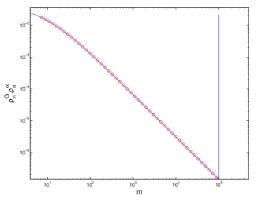
Figure 3: Log-log pot of the marginal probability distribution for the slicer map $S_{1/3}$ as a function of the position of the $m$-th cell at fixed time $n=10^{5}$. $\rho_{n}^{G}(m)$ denotes the coarse grained distribution obtained from our exact analytical results Eqs.(50,51) (continuous line). It is compared with the asymptotic analytical approximation $\rho_{n}^{\alpha}(m)$, Eq.(52) (dotted line). Apart from the values at $m=n$, where $\rho_{n}^{G}$ has a spike due to the travelling area, the asymptotic functional forms coincide.

III A simple stochastic model of slicer diffusion?

Since deterministic dynamical systems often generate a type of randomness, it is frequently attempted to match their dynamics to simple stochastic processes for understanding their transport properties Do99 ; Gasp ; Kla06 ; RoMM07 ; CFLV08 . However, as we pointed out in the introduction, for diffusion in polygonal billiards such a stochastic modeling turned out to be surprisingly non-trivial Zas02 ; LWWZ05 ; Kla06 ; Dett14 . Motivated by this line of research, in this section we relate the slicer diffusion to known stochastic models of anomalous diffusion.

We first summarize our main results for diffusive transport generated by our non-chaotic slicer map under variation of the control parameter $0\leq\alpha\leq 2$. In the limit of $n\to\infty$ we have:

1. $\alpha=0$: ballistic motion with MSD $\langle\Delta\hat{X}^{2}_{n}\rangle\sim n^{2}$

2. $0<\alpha<1$: superdiffusion with MSD $\langle\Delta\hat{X}^{2}_{n}\rangle\sim n^{2-\alpha}$

3. $\alpha=1$: normal diffusion with linear MSD $\langle\Delta\hat{X}^{2}_{n}\rangle\sim n$

4. $1<\alpha<2$: subdiffusion with MSD $\langle\Delta\hat{X}^{2}_{n}\rangle\sim n^{2-\alpha}$

5. $\alpha=2$: logarithmic subdiffusion with MSD $\langle\Delta\hat{X}^{2}_{n}\rangle\sim\log n$

6. $\alpha>2$: localisation in the MSD with $\langle\Delta\hat{X}^{2}_{n}\rangle\sim const.$

Additionally, Theorem 2 gives information about the asymptotic behavior of all higher order even moments scaling as $\langle\Delta\hat{X}^{p}_{n}\rangle\sim n^{p-\alpha}$ in the long time limit for $p>2$ and $0<\alpha\leq 2$.

As recently highlighted in Refs. KHL10 ; HKL14 , there do not seem to exist too many stochastic models exhibiting a transition from subdiffusion over normal diffusion to superdiffusion under parameter variation: We are aware of a specific continuous time random walk (CTRW) model ZuKl95 , (generalized) elephant walks KHL10 ; HKL14 , and generalized Langevin equations (gLe) including fractional Brownian motion PWM96 ; TCK10 ; JM10 . For these models one can easily check that there is no simple matching between their diffusive properties and the above scenario representing slicer diffusion. That is, the scaling of the MSD with parameters by switching between all diffusive regimes is generically different from the slicer dynamics, and/or more than one control parameter is needed to change the diffusive properties. However, for both the CTRW and the gLe there is a partial matching to the slicer diffusion in specific diffusive regimes to which we come back below. Meaning so far we are not aware of any stochastic model that (asymptotically) reproduces the slicer diffusion by exhibiting all the different diffusive regimes listed above under single parameter variation.

For all the stochastic models just mentioned the dynamics is generated by temporal randomness, that is, random variables are drawn in time from given probability distributions. A second fundamental class of stochastic models is defined by spatial randomness of the positions of scatterers with a point particle moving between them. An important example is the one-dimensional stochastic Lévy Lorentz gas (LLg) BFK00 ; BF99 ; BCV10 : Here a point particle moves ballistically between static point scatterers arranged on a line from which it is either transmitted or reflected with probability $1/2$. The distance $r$ between two consecutive scatterers is a random variable drawn independently and identically distributed from a Lévy distribution,

$$\lambda(r)\equiv\beta r_{0}^{\beta}\frac{1}{r^{\beta+1}},\ \ r\in\left[r_{0},+\infty\right)\>,$$ (53)

where $\beta>0$ and $r_{0}$ is a cutoff fixing the characteristic length scale of the system. The LLg shares a basic similarity with the slicer map in that its scatterers are positioned according to the same asymptotic functional form as the slicers, see Eq.(2). On the other hand, the slicer positions are deterministic while the LLg scatterers are distributed randomly. In more detail, the slicers amount to transition probabilities for nearest neighbour jumps on a periodic lattice that decrease by a power law while in the LLg the jumps follow a power law distribution with trivial transition probabilites at random scatterers. Finally, the slicer dynamics is discrete in time while the LLg is a time-continuous system.

From these facts it follows that there exists an intricate dependence on initial conditions in the LLg that is not present that way in the slicer map: The LLg diffusive properties depend on whether a walker starts anywhere on the line, which means typically between two scatterers, called equilibrium initial condition, or exactly at a scatterer, called nonequilibrium initial condition BFK00 ; BCV10 . In BFK00 bounds for the MSD have been calculated in both cases. Interestingly, the lower bound for equilibrium initial conditions was obtained from CTRW theory on which we will elaborate further below.

The results for nonequilibrium conditions have been improved in BCV10 based on simplifying assumptions by which asymptotic results for the position probability distribution of the moving particle could be calculated. It was shown that the LLg only displays superdiffusion, which as in the slicer map is governed by traveling (in BCV10 called subleading) and sub-traveling (in BCV10 called leading) contributions. However, while in the slicer map both these contributions scale in the same way for the MSD, cf. Remark 4, for the LLg they yield different scaling laws depending on the order of the moment $p$ and the control parameter $\beta$. These different regimes are deeply rooted in the different physics of the system featuring an intricate interplay between different length scales. As a consequence, the LLg MSD displays three different regimes with an exponent determined by three different functions of $\beta$, cf. Eq.(3) in BCV10 . All higher order moments could also be calculated for the LLg. Very interestingly, Eq.(13) in BCV10 and all even moments of the slicer map, cf. Theorem 2, exactly coincide by a piecewise transformation between $\beta\in(0,3/2]$ and $\alpha\in(0,1]$. In other words, for every $\beta$ in BCV10 it suffices to fix the slicer’s parameter $\alpha$ so that one of the moments (e.g. the second) matches, to match all other moments as well . Then the asymptotic form of the moments $\langle r^{p}(t)\rangle$ for all $p>0$ is given by

$$\langle r^{p}(t)\rangle\sim\left\{\begin{array}[]{rl}t^{\frac{p}{1+\beta}}\leavevmode\nobreak\ ,&\ \mbox{if }\beta<1,\ p<\beta\\ t^{\frac{p(1+\beta)-\beta^{2}}{1+\beta}}\leavevmode\nobreak\ ,&\ \mbox{if }\beta<1,\ p>\beta\\ t^{\frac{p}{2}}\leavevmode\nobreak\ ,&\ \mbox{if }\beta>1,\ p<2\beta-1\\ t^{\frac{1}{2}+p-\beta}\leavevmode\nobreak\ ,&\ \mbox{if }\beta>1,\ p>2\beta-1\end{array}\right.\>.$$ (54)

Surprisingly they can be matched with the slicer moments in Eq.(36) by taking

$$\alpha=\left\{\begin{array}[]{rl}{\beta^{2}}/{(1+\beta)}&\ \ \mbox{if }0<\beta\leq 1\\ \beta-{1}/{2}&\ \ \mbox{if }1<\beta\leq\frac{3}{2}\\ 1&\ \ \mbox{if }\beta>\frac{3}{2}\end{array}\right.\>.$$ (55)

This means that by using the above transformation both processes are asymptotically indistinguishable from the viewpoint of these moments, meaning the slicer map generates a kind of LLg-type walk in the superdiffusive regime if the available information on the system (the observables) include the moments only. On the other hand, the transformation is piecewise which reflects the different functional forms for the exponent of the moments in the LLg while for the slicer map only one such functional form exists. Indeed, it is well known that the moments carry only partial information on the properties of (anomalous) transport phenomena, and that knowledge of correlations is necessary to distinguish one class of stochastic processes from another KRS08 ; Sokolov .

Another interesting fact within this context is that for the traveling region alone (called ballistic contribution in BFK00 ) the MSD of the LLg scales as $\sim t^{2-\beta}$ in continuous time $t$, as was shown in BFK00 . Formally, this result matches exactly to the MSD of the slicer map of $\sim n^{2-\alpha}$ as calculated in Proposition 1. Note also that the slicer positions generate a probability distribution for the sub-traveling region of ${\rho}^{G}_{n}(j)\sim|j|^{-\alpha-1}$, see Remark 2, which matches to $\lambda(r)$ of the LLg Eq. (53).

We now comment on similarities and differences of the slicer diffusion with CTRW theory. For equilibrium initial conditions in the LLg it was shown that for $1<\beta<2$ the MSD is bounded from below by $\sim t^{3-\beta}$ BFK00 . However, this is exactly the result for a Lévy walk modeled by CTRW theory ZuKl95 . Even more, results for all higher Lévy walk CTRW moments were recently calculated to $\sim t^{p+1-\beta}$ for $p>\beta$, see Eq.(18) in RSHB14 . With $\beta=1+\alpha$ the slicer superdiffusion thus formally (also) matches to Lévy walk diffusion defined by CTRW theory. On the other hand, from a conceptual point of view a CTRW is constructed very differently from both the LLg and the slicer map dynamics. Hence, it is not very clear why a CTRW mechanism should apply in both these cases. Another remark is that for the superdiffusive regime of the slicer diffusion of $0\leq\alpha<1$ the frozen Lévy distribution according to which the transition probabilities have been defined does not belong to the parameter regime for which such distributions are stochastically stable in the sense of a generalized central limit theorem MeKl00 ; KRS08 , which holds only for $1<\alpha\leq 3$. This points again at a crucial difference between slicer dynamics and CTRW theory, where for the latter the resulting probability distributions are stochastically stable. Our discussion suggests that there is a more intricate interplay between the Lévy potential we want to mimic, the dynamics we use to obtain it, and the power law distributions we generate from it.

We conclude this section by a remark on a curious similarity between the slicer diffusion in the subdiffusive regime and Gaussian stochastic processes. It was shown in Refs. PWM96 ; TCK10 ; ChKl12 that for a gLe with power law memory kernels for friction and/or noise the MSD exhibits a transition from a constant over $\sim\log n$ to subdiffusion in the long time limit. Especially, for an overdamped gLe with Gaussian noise governed by a power law anti-persistent memory kernel $\sim-t^{-\gamma}$ the MSD was calculated to $\sim t^{2-\gamma}$ for $1<\gamma<2$, $\sim\log t$ for $\gamma=2$ and $\sim const.$ for $\gamma>2$ ChKl12 . Formally these results match exactly to the slicer MSD for $1<\alpha$, cf. Proposition 1. However, this overdamped gLe does not exihibit any superdiffusion. And as the probability distributions generated by such a gLe are strictly Gaussian in the long time limit there is, again, a clear conceptual mismatch to the slicer dynamics: In the gLe the subdiffusion is generated from power law memory in the random noise (by calculating the MSD via the Taylor-Green-Kubo formula PWM96 ; TCK10 ; ChKl12 ) while for the slicer map the anomalous dynamics was calculated from non-Gaussian probability distributions. We remark that so far nothing is known about the correlation decay in the slicer dynamics; for the LLg it is very complicated BF99 . Hence, while formally there might be a similar mechanism in gLe and slicer dynamics for generating subdiffusion, again, conceptually these dynamics are very different.

To summarize this section, to our knowledge currently there is no stochastic model that fully reproduces the slicer diffusion. The superdiffusive slicer regime formally matches to diffusion known from Lévy walks, as reproduced both by the LLg and CTRW theory, although in detail the parameter dependences for the MSD generated by both models are different. The subdiffusive regime formally matches to what is generated by a gLe with power law correlated Gaussian noise. Conceptually all these stochastic models are very different from the slicer model, hence any similarity is purely formal and not supported from first principles. Based on this analysis it is tempting to conclude that one may need a correlated CTRW model to stochastically reproduce the slicer diffusion, or perhaps alternatively a simple Lévy Markov chain model.

The reason why we elaborated so explicitly on a possible stochastic modeling of the slicer dynamics is that our analysis might help to understand the reason for the controversy of how to stochastically model diffusion in polygonal billiards Zas02 ; LWWZ05 ; Kla06 ; Dett14 . With the slicer map we are trying to capture a basic mechanism generating diffusion in these systems. However, as we showed above, the slicer diffusion seems to share features with generically completely different stochastic models depending on parameter variation. This might help to explain why different groups of researchers came to contradicting conclusions for modeling diffusion in polygonal billiards (not from first principles) by applying different types of stochastic processes.

IV Concluding remarks

In search of mathematically tractable deterministic models of normal and anomalous diffusion, which may shed light on the minimal mechanisms generating different transport regimes in non-chaotic systems, we have introduced a new model which we called the slicer map. This map mimics in a one dimensional space main features that distinguish periodic polygonal billiards from other models of transport, namely the complete absence of randomness and of positive Lyapunov exponents, and a sequence of splittings of a beam of particles due to collisions at singularities of the billiard walls. As observed in Refs. ArGuRe00 ; ARV03 ; SchSt06 ; JeRo06 ; SaLa06 ; JBR08 , in these cases the geometry determines the transport law, differently from standard hydrodynamics in which the geometry only yields the boundary conditions. Therefore the rule according to which the polygonal scatterers are distributed in space plays a crucial role. Here we have investigated the case of a specific deterministic rule modeling diffusion in polygonal billiards.

In our one-dimensional slicer model $S_{\alpha}$ the effect of the billiard geometry, which “slices” beams of particles ever more finely further and further away from the origin, is produced by the rate at which the size of the slices decreases with the position, i.e. by the value of a single control paraemeter $\alpha$. For instance, $\alpha={1}/{3}$ yields for the MSD and for the even higher order moments $\langle\Delta\widehat{X}^{2}(n)\rangle\ \sim n^{\frac{5}{3}}\quad\mbox{and}\quad\langle\Delta\widehat{X}^{p}(n)\rangle\sim n^{\frac{3p-1}{3}}$ for long times. As we have discussed, the $n^{5/3}$ behavior coincides with the asymptotic MSD estimated numerically for a periodic polygonal channel made of parallel walls which form angles of $90$ degrees JeRo06 ; JBR08 for which one would naively expect ballistic behaviour.

It seems there do not exist too many models, neither in terms of deterministic nor stochastic dynamics, that exhibit sub-, super- and normal diffusive regimes under single parameter variation. The slicer map adds a new facet to this rather rare collection, as it generates all these different types of diffusion in a strictly deterministic and non-chaotic way. This suggests a mechanism explaining why in computer simulations of polygonal billiards so many different types of diffusion have been observed under parameter variation ArGuRe00 ; ARV03 ; SchSt06 ; JeRo06 ; SaLa06 ; JBR08 . It may also help to explain the severe difficulties to model diffusion in such systems by a single, sufficiently simple anomalous stochastic process: We have argued that, depending on the value of its control parameter, the slicer diffusion matches mathematically to what is generated by very different classes of stochastic processes, which is in line with findings for polygonal billiard diffusion.

It would be highly desirable to construct a simple stochastic process reproducing the full range of the slicer diffusion. It would also be important to extract a slicer map from a given polygonal billiard starting from first principles. This would enable to check whether a slicing mechanism similar to the one proposed here in terms of a power law distribution of slicers is realistic. Correlation functions for the slicer map need to be calculated in order to fully appreciate its dynamics. And as the slicer map is analytically tractable, our model invites to play around with variations of the slicer idea for better understanding the origin of non-chaotic diffusion.

Acknowledgements:

The authors are grateful to Raffaella Burioni for illuminating remarks. LR acknowledges funding from the European Research Council, 7th Framework Programme (FP7), ERC Grant Agreement no. 202680. The EC is notresponsible for any use that might be made of the data appearing herein. CG acknowledges financial support from the MIUR through FIRB project “Stochastic processes in interacting particle systems: duality, metastability and their applications”, grant n. RBFR10N90W and the Institut Henry Poincaré for hospitality during the trimester “Disordered systems, random spatial processes and some applications”.

Bibliography

Bibliography

- (1) J.R. Dorfman. An introduction to chaos in nonequilibrium statistical mechanics. Cambridge University Press, Cambridge, 1999.
- (2) P. Gaspard. Chaos, scattering, and statistical mechanics. Cambridge University Press, Cambridge, 1998.
- (3) R. Klages. Microscopic chaos, fractals and transport in nonequilibrium statistical mechanics, volume 24 of Advanced Series in Nonlinear Dynamics. World Scientific, Singapore, 2007.
- (4) L. Rondoni and C. Mejia-Monasterio. Nonlinearity, 20:R1, 2007.
- (5) P. Castiglione, M. Falcioni, A. Lesne, and A. Vulpiani. Chaos and Coarse Graining in Statistical Mechanics. Cambridge University Press, Cambridge, 2008.
- (6) U. Marini Bettolo Marconi, A. Puglisi, L. Rondoni, A. Vulpiani. Phys. Rep., 461:11, 2008.
- (7) O.G. Jepps, L. Rondoni. J. of Phys. A, 43:P05015, 2010
- (8) G.M. Zaslavsky. Phys. Rep., 371:461, 2002.
- (9) R. Klages, G. Radons, and I.M. Sokolov, editors. Anomalous Transport: Foundations and Applications. Wiley-VCH, Berlin, 2008.
- (10) O.G. Jepps, S.K. Bathia, D.J. Searles. Phys. Rev. Lett. 91:126102, 2003
- (11) A. Igarashi, L. Rondoni, A. Botrugno, M. Pizzi. Commun. Theor. Phys. 56:352, 2011
- (12) O.G. Jepps and L. Rondoni. J. Phys. A: Math. Gen., 39:1311, 2006.
- (13) O.G. Jepps, C. Bianca, and L. Rondoni. Chaos, 13:013127, 2008.
- (14) I.M. Sokolov. Soft Matter 8:9043, 2012.
- (15) R. Metzler and J. Klafter. Phys. Rep., 339:1, 2000.
- (16) G. Zumofen and J. Klafter. Phys. Rev. E, 51:1818, 1995.
- (17) N. Korabel and R. Klages. Phys. Rev. Lett., 89:214102, 2002.
- (18) N. Korabel and R. Klages. Physica D, 187:66, 2004.
- (19) T. Manos and M. Robnik. Phys. Rev. E, 89:022905, 2014.
- (20) B. Li and L. Wang and B. Hu. Phys. Rev. Lett., 88:223901, 2002
- (21) B. Li, J. Wang, L. Wang, and G. Zhang. Chaos, 15:015121, 2005.
- (22) Carl P. Dettmann. Commun. Theor. Phys., 62:521, 2014.
- (23) R. Artuso, I. Guarneri, and L. Rebuzzini. Chaos, 10:189, 2000.
- (24) D. Alonso, A. Ruiz, and I. de Vega. Physica D, 187:184, 2004.
- (25) M. Schmiedeberg and H. Stark. Phys. Rev. E, 73:031113/1–9, 2006.
- (26) D.P. Sanders and H. Larralde. Phys. Rev. E, 73:026205, 2006.
- (27) J. Hardy and J. Weber. J. Math. Phys., 21:1802, 1980.
- (28) V. Delecroix, P. Hubert, and S. Lelièvre. Ann. Scient. Ec. Norm. Sup. 4e serie, t. 47, 1085 (2014).
- (29) J.H. Hannay and R.J. McCraw. J. Phys. A: Math. Gen., 23:887, 1990.
- (30) E. Gutkin. J. Stat. Phys., 83:7, 1996.
- (31) G.M. Zaslavsky and M. Edelman. Chaos, 11:295, 2001.
- (32) C.P. Dettmann and E.G.D. Cohen. J. Stat. Phys., 101:775, 2000.
- (33) F. Cecconi, M. Falcioni, A. Vulpiani, and D. del Castillo-Negrete. Physica D, 180:129, 2003.
- (34) S. Denisov, J. Klafter, and M. Urbakh. Phys. Rev. Lett., 91:194301, 2003.
- (35) E. Barkai and V. Fleurov. J. Stat. Phys., 96:325, 1999.
- (36) E. Barkai, V. Fleurov, and J. Klafter. Phys. Rev. E, 61:1164, 2000.
- (37) R. Burioni, L. Caniparoli, and A. Vezzani. Phys. Rev. E, 81:060101(R), 2010.
- (38) P. Barthelemy, J. Bertolotti, and D.S. Wiersma. Nature, 453:495, 2008.
- (39) N. Kumar, U. Harbola, and K. Lindenberg. Phys. Rev. E, 82:021101, 2010.
- (40) U. Harbola, N. Kumar, and K. Lindenberg. Phys. Rev. E, 90:022136, 2014.
- (41) J.M. Porra, K.-G. Wang, and J.Masoliver. Phys. Rev. E, 53:5872, 1996.
- (42) A. Taloni, A.V. Chechkin, and J. Klafter. Phys. Rev. Lett., 104:160602, 2010.
- (43) J.-H. Jeon and R. Metzler. Phys. Rev. E, 81:021103, 2010.
- (44) A. Rebenshtok, S. Denisov, P. Hänggi, and E. Barkai. Phys. Rev. Lett., 112:110601, 2014.
- (45) A.V. Chechkin, F. Lenz, and R. Klages. J. Stat. Mech.: Theor. Exp., 2012:L11001, 2012.