Radiative transfer model for contaminated slabs : experimental validations

Abstract

This article presents a set of spectro-goniometric measurements of different water ice samples and the comparison with an approximated radiative transfer model. The experiments were done using the spectro-radiogoniometer described in Brissaud et al. (2004). The radiative transfer model assumes an isotropization of the flux after the second interface and is fully described in Andrieu et al. (2015).

Two kind of experiments were conducted. First, the specular spot was closely investigated, at high angular resolution, at the wavelength of $1.5\,\mbox{$\mu$m}$ , where ice behaves as a very absorbing media. Second, the bidirectional reflectance was sampled at various geometries, including low phase angles on 61 wavelengths ranging from $0.8\,\mbox{$\mu$m}$ to $2.0\,\mbox{$\mu$m}$ .

In order to validate the model, we made a qualitative test to demonstrate the relative isotropization of the flux. We also conducted quantitative assessments by using a bayesian inversion method in order to estimate the parameters (e.g. sample thickness, surface roughness) from the radiative measurements only. A simple comparison between the retrieved parameters and the direct independent measurements allowed us to validate the model.

We developed an innovative bayesian inversion approach to quantitatively estimate the uncertainties on the parameters avoiding the usual slow Monte Carlo approach. First we built lookup tables, and then searched the best fits and calculated a posteriori density probability functions. The results show that the model is able to reproduce the spectral behavior of water ice slabs, as well as the specular spot. In addition, the different parameters of the model are compatible with independent measurements.

Various species of ices are present throughout the Solar System. From water ice and snow on Earth to nitrogen ice on Triton (Zent et al., 1989), not forgetting carbon dioxide ice on Mars (Leighton and Murray, 1966). Ice an snow covered areas have a strong impact on planetary climate dynamics, as they can lead to significant regional scale albedo changes at the surface and surface/atmosphere volatiles interactions. The physical properties of the cover have also an impact on the energy balance : for example the albedo depend on the grain size of the snow (Dozier et al., 2009; Negi and Kokhanovsky, 2011), on the roughness of the interface (Lhermitte et al., 2014) on the presence or not and the physical properties of impurities (Dumont et al., 2014), or on the specific surface area (Picard et al., 2009; Mary et al., 2013). The study and monitoring of theses parameters is a key to constrain the energy balance of a planet.

Radiative transfer models have proven essential to retrieve such properties and their evolution at a large scale, and different families exist. Ray tracing algorithms, such as those described in Picard et al. (2009) for snow or Pilorget et al. (2013) for compact polycrystalline ice simulate the complex path of millions of rays into the surface. They provide very accurate simulations, but have the weakness of being time consuming. Analytical solutions of the radiative transfer in homogeneous granular media have been developed for example by Shkuratov et al. (1999) and Hapke (1981). They are fast, and when the surface cannot be described as homogeneous, they must be combined with another family of techniques such as discrete ordinate methods like DISORT (Stamnes et al., 1988). These methods have been widely studied on Earth snow (Carmagnola et al., 2013; Dozier et al., 2009; Dumont et al., 2010; Painter and Dozier, 2004) and other planetary cryospheres (Appéré et al., 2011; Eluszkiewicz and Moncet, 2003), modeling a granular surface. Compact polycrystalline ices have however been recognized to exist on several objects : CO₂ on Mars (Kieffer and Titus, 2001; Eluszkiewicz et al., 2005), N₂ on Triton and Pluto, (Zent et al., 1989; Eluszkiewicz and Moncet, 2003) and probably SO₂ on Io (Eluszkiewicz and Moncet, 2003), owing to the very long light path-lengths measured, over several decimeters. Radiative transfer in compact slabs is different from in granular media. We developed an approximated model (Andrieu et al., 2015) designed to study contaminated ice slabs, with a fast numerical implementation, that has already been numerically validated. The main objective of the model is the analysis of massive spectro-imaging planetary data of these surfaces. For this purpose, it is semi analytic and fast implemented. It is designed to retrieve the variations of thickness and impurity content of compact polycrystalline planetary ices.

In the present article, we will test the accuracy of this approximated model on laboratory spectroscopic measurements of pure water ice Bidirectional Reflectance Distribution Function (BRDF). The goal is to propose an inversion framework to retrieve surface properties, including uncertainties in order to demonstrate the validity of the approach. In order to speed up the inversion, we based the algorithm on look-up tables that minimize the computation time of the direct model. This strategy will be very useful to analyze real hyperspectral images. The thickness of ice estimated from the inversion is validated in comparison to real direct measurements. Also the specular lobe is adjusted to demonstrate that the model is able to reasonably fit the data with a coherent roughness value.

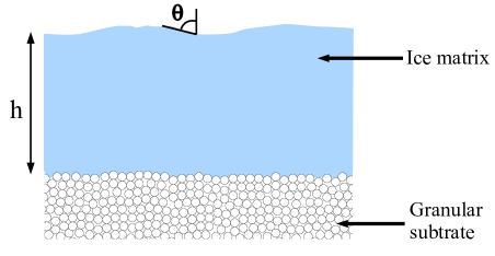
Figure 1: Scheme of the surface representation in the radiative transfer model applied on the laboratory measurements. $h$ represents the slab thickness. $\bar{\theta}$ represent the mean slope to describe the surface roughness.

1 Description of the model

The model, Andrieu et al. (2015), is inspired from an existing one described in Hapke (1981) and Douté and Schmitt (1998), that simulates the bidirectional reflectance of stratified granular media. It has been adapted to compact slab, contaminated with pseudo-spherical inclusions, and a rough top interface. In the context of this work, we suppose a layer of pure slab ice, overlaying an optically thick layer of granular ice, as described on figure 1. The roughness of the first interface is described using the probability density function of orientations of slopes defined in Hapke (1984). This distribution of orientations is fully described by a mean slope parameter $\bar{\theta}$. The ice matrix is described using its optical constants and it thickness. Within the slab, the model can also incorporate inclusions, supposed to be close to spherical and homogeneously distributed inside the matrix. They are described by their optical constants, their volumetric proportions and their characteristic grain-sizes. There can be several different types of inclusions. Each type can be of any material, except the one constituting the matrix : it can be any other kind of ice, mineral, or even bubbles.

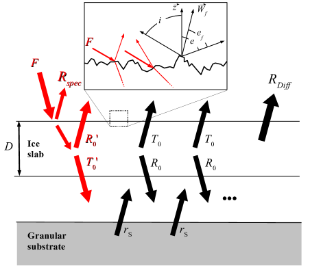
Figure 2: Illustration of the radiative transfer in the surface. Anisotropic transits are represented in red. $\vec{F}$ is the incident radiation flux, $R_{spec}$ and $R_{Diff}$ are respectively the specular and diffuse contributions to the reflectance of the surface. $r_{s}$ is the lambertian reflectance of the granular substrate, and $R_{0}$ and $T_{0}$ are total reflexion and transmission factors of the slab layer. A prime indicates an anisotropic transit. The reflection and transmission factors are different in isotropic or anisotropic conditions. The granular and slab layers are artificially separated in this figure to help the understanding of the coupling between the two layers. On the top : illustration of the reflections and transmission at the first interface, used in the calculations of $R_{spec}$ and the determination of the amount of energy injected in the surface. $\vec{z}$ is the normal to the surface, $\vec{W}_{f}$ the local normal to a facet, $i$ and $e$ are respectively the incidence and emergence angle, and $e_{f}$ is the local emergence angle for a facet. Each different orientation of a facet will lead to a different transit length in the slab. A more detailed description can be found in Andrieu et al. (2015).

Figure 2 illustrates the general principle of the model. The simulated bidirectional reflectance results from two separate contributions: specular and diffuse. The specular contribution of a measurement is estimated from the roughness parameter, the optical constants of the matrix, and the apertures of the light source and the detector. The surface is considered as constituted of many unresolved facets, which orientations follow the defined probability density function. The specular reflectance is obtained integrating every reflection on the different facets. The total reflection coefficient at the first rough interface is obtained by integrating specular contributions in every emergent direction, at a given incidence. This gives the total amount of energy transmitted into the system constituted of the contaminated slab and the substrate. The diffuse contribution is then estimated solving the radiative transfer equation inside this system under various hypothesis. It is considered that : (i) the first transit through the slab is anisotropic due to the collimated radiation from the source, and that there is an isotropization at the second rough interface (i.e. when the radiation reach the semi-infinite substrate). For the refraction and the internal reflection, every following transit is considered isotropic. (ii) the geometrical optics are valid. This means that the size of the inclusions and the thickness of the slab layer must be larger than the considered wavelength. (iii) the inclusions inside the matrix are close to spherical and homogeneously distributed. The reflexion and transmission factors of the layers are obtained using an analytical estimation of Fresnel coefficients described in Chandrasekhar (1960); Douté and Schmitt (1998), and a simple statistical approach, detailed in Andrieu et al. (2015). The contribution of the semi infinite substrate is described by its single scattering albedo. Finally, as the slab layer is under a collimated radiation from the light source, and under a diffuse radiation from the granular substrate, the resulting total bidirectional reflectance is computed using adding doubling formulas.

2 Data

2.1 Spectro-radiogoniometer

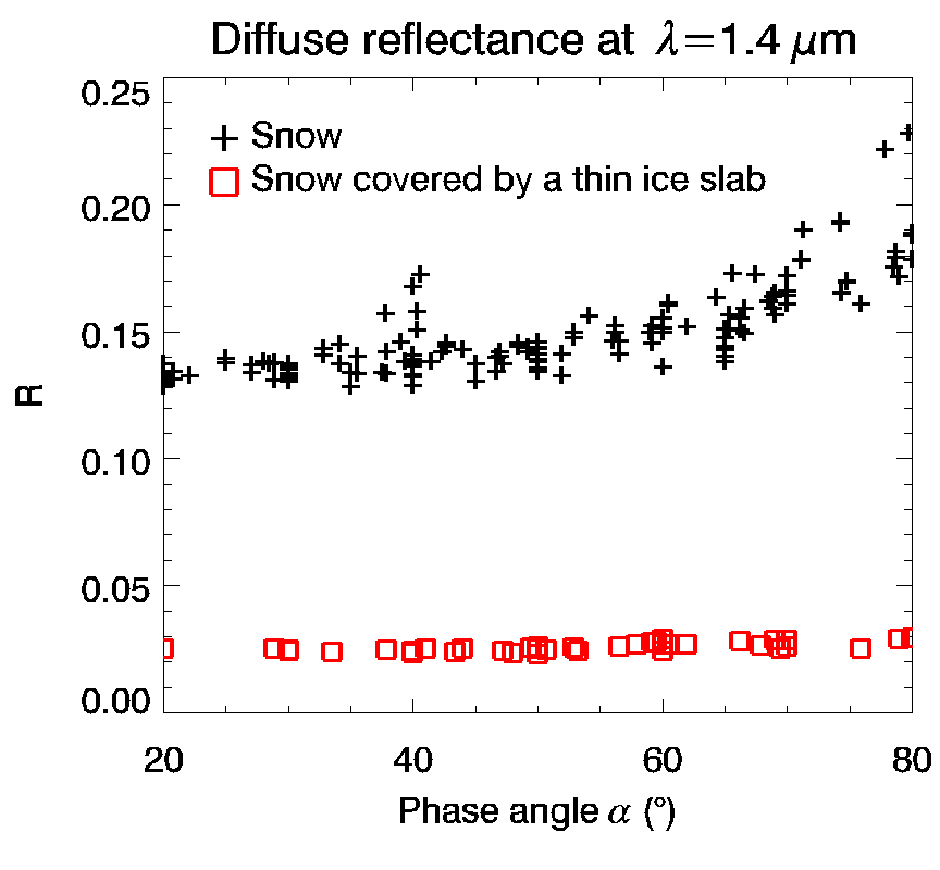
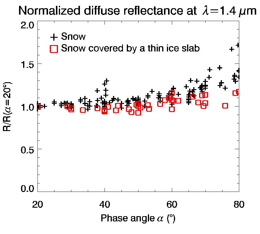
(a) (b)

Figure 3: (a) Reflectance factor at a wavelength $\lambda=1.4\,\mbox{$\mu$m}$versus phase angle for snow only (black crosses) and the same snow, but covered with a $1.42\pm 0.27\,\mbox{mm}$ water ice slab (red squares). The thin layer of slab ice not only lower the level of reflectance as expected, but also seems to isotropize the reflected radiation. It is clearer on plot (b), that represents the same data, but normalized by the value at a phase angle $\alpha=20\text{\textdegree}$. This data shows that even a very thin layer of ice has a strong effect on the directivity of the surface. This justify the approximation of isotropization at the second interface supposed by the model, and the description of the substrate using only its single scattering albedo.

The bidirectional reflectance spectra were measured using the spectrogonio-radiometer from IPAG fully described in Brissaud et al. (2004). We collected spectra in the near infrared at incidences ranging from $40\text{\textdegree}$ to $60\text{\textdegree}$, emergence angles from $0\text{\textdegree}$ to $50\text{\textdegree}$, and azimuth angles from $0\text{\textdegree}$ to $180\text{\textdegree}$. The sample is illuminated with a large monochromatic beam (divergence $<1\text{\textdegree}$) an the near infrared spectrum covering the range from $0.800\,\mbox{$\mu$m}$ to $4800\,\mbox{$\mu$m}$ is measured by an InSb photovoltaic detector. This detector has a nominal aperture of $4.2\text{\textdegree}$, that result in a field of view on the sample of approximately $20\,mm$ in diameter. The minimum angular sampling of illumination and observation directions is $0.1\text{\textdegree}$, with a reproducibility of $0.002\text{\textdegree}$. In order to avoid azimuthal anisotropy, the sample is rotated during the acquisition. The sample rotation axis may be very slightly misadjusted, resulting on a notable angular drift on the emergence measured up to $1\text{\textdegree}$.

2.2 Ice BRDF measurements

The ice samples were obtained by sawing artificial columnar water ice in sections. These sections were put on top of an optically thick layer of compacted snow, that was collected in Arselle, in the French Alps. The spectral measurements were conducted in a cold chamber at 263K. Still, the ice and the snow were unstable in the measurement’s environment, due to the dryness of the chamber’s atmosphere. The grain-size of the snow showed an evolution and the thickness of a given slab showed a decrease of $0.343\,\mbox{mm/day}$. Each sample needs a acquisition time of $10\,\mbox{hours}$. For each measurement, the ice slab was sliced, and its thickness was measured in five different locations. It was then set on top of the snow sample, and this system was put into the spectro-goniometer, and put into rotation for the measurement. As the surface is not perfectly plane, the measured thickness is not constant. This results in an $2\sigma$ standard-deviation in the measurement of the thickness than ranges from $0.54\,\mbox{mm}$ to $2.7\,\mbox{mm}$ in our study, depending on the sample.

Specular contribution

The specular contribution was measured on a $12.51\,\mbox{mm}$ thick slab sample on top of Arselle snow. This sample is the same sample that sample 3 described in the next paragraph. The illumination was at an incidence angle of $50\text{\textdegree}$, and 63 different emergent geometries were sampled, ranging from $45\text{\textdegree}$ to $55\text{\textdegree}$ in emergence, and from $170\text{\textdegree}$ to $180\text{\textdegree}$ in azimuth. A measure at the wavelength of $1.5\,\mbox{$\mu$m}$ is represented on figure 5 (a). The sampling is $1\text{\textdegree}$ in emergence and azimuth within $47\text{\textdegree}$ and $53\text{\textdegree}$ in emergence and $175\text{\textdegree}$ and $180\text{\textdegree}$ in azimuth.

Diffuse reflectance spectra

The diffuse contribution was measured on three samples of different slab thickness. The three thicknesses were measured on different locations of the samples with a caliper before the spectrogonio measurement, resulting in $h_{1}=1.42\pm 0.47\,\mbox{mm}$, $h_{2}=7.45\pm 0.84\,\mbox{mm}$, $h_{3}=12.51\pm 2.7\,\mbox{mm}$, respectively for samples 1, 2 and 3, with errors at $2\sigma$. $61$ wavelengths were sampled ranging from $0.8\,\mbox{$\mu$m}$ to $2.0\,\mbox{$\mu$m}$. Spectra were collected on 39 different points of the BRDF, respectively for the incidence, emergence and azimuth angles : $\left[40\text{\textdegree},50\text{\textdegree},60\text{\textdegree}\right]$, $\left[0\text{\textdegree},10\text{\textdegree},20\text{\textdegree}\right]$ and $\left[0\text{\textdegree},45\text{\textdegree},90\text{\textdegree},140\text{\textdegree},160\text{\textdegree},180\text{\textdegree}\right]$. This set of angles results in only 39 different geometries because the azimutal angle is not defined for a nadir emergence.

Snow diffuse reflectance spectra

Diffuse reflectance spectra of natural snow only were also measured. The objective was to estimate the effect of a slab layer on the BRDF. Figure 3 show on the same plots the reflectance factor versus phase angle of the snow and the snow covered with a $1.42\,\mbox{mm}$ thick ice slab (sample 1). It illustrates the two most notable effects of a thin layer of slab ice on top of an optically thick layer of snow. The most intuitive effect is to lower the level of reflectance : it is due to absorption during the long optical path lengths in the compact ice matrix. The second is that the radiation is more lambertian than the one of only snow. This data gives credit to the first hypothesis of isotropization of the radiation formulated in the model (see Section 1). The description of the bottom granular layer as isotropic, defined only its single scattering albedo, may be considered brutal, but this dataset shows that a thin coverage of slab ice even on a very directive material such as snow, is enough to strongly flatten the BRDF.

3 Method

We designed an inversion method aiming at massive data analysis. This method consists in two steps : first the generation of a synthetic database that is representative of the variability of the model, and then comparison with actual data. To generate the synthetic database, we used optical constants for water ice at $270\,\mbox{K}$. The $7\,\mbox{K}$ difference between the actual temperature of the room and the temperature assumed for the optical constants has negligible effect. We combined the datasets of Warren and Brandt (2008) and Schmitt et al. (1998) making the junction at $1\,\mbox{$\mu$m}$, the former set for the shorter wavelengths, and the latter for the wavelengths larger than $1\,\mbox{$\mu$m}$.

In order to validate the model on the specular reflection from the slab, we chose to use the reflectance at $1.5\,\mbox{\text{$\mu$}m}$, where the ice is very absorbing. Figures 4, and 5 clearly demonstrate that there is negligible diffuse contribution in geometry outside the specular lobe from the sample with $12.51\,\mbox{mm}$ thick pure slab. Thus, the roughness parameter $\bar{\theta}$ is the only one impacting the reflectance in the model. We chose to inverse this parameter first, and validate the specular contribution.

We will then focus on the validation in the spectral domain, for the diffuse contribution. We will use the estimation of the roughness parameter $\bar{\theta}$ obtained earlier and the spectral data in order to estimate the slab thickness and the grain-size of the snow substrate. To do this, we assumed that the roughness was not changing significantly enough to have a notable impact on diffuse reflectance from one sample to another. This assumption is justified by the fact that the different columnar ice samples were made the same way, as flat as possible and the low value of $\bar{\theta}$ retrieved as discussed in the next section. It is confirmed by the results of section 3.2, that suggest a very low roughness, as expected. Such low roughness parameter have negligible influence on the amount of energy injected into the surface.

3.1 Inversion strategy

The inversion consists in estimating the model parameter $m$ from the model $F(m)$, that are close to the data $d$. Tarantola (1982) showed that it can be mathematically solved by considering each element as a Probability Density Function (PDF) . In non-linear direct problem, the solution may not be analytically approached. Nevertheless, it is possible to sample the solution PDF with a Monte Carlo approach as shown in Mosegaard and Tarantola (1995), but this solution is very time consuming.

The actual observation is considered as prior information on data $\rho_{D}(d)$ in the observation space $D$. It is assumed to be a $N$-dimension gaussian PDF $\mathcal{G}(d_{mes},\overline{\overline{C}})$, with mean $d_{mes}$ and covariance matrix $\overline{\overline{C}}$. The values $r_{i}$ are the observations for each element (angular or spectral as described later). The covariance matrix $\overline{\overline{C}}$ is assumed here to be diagonal since measurements at a given geometry/wavelength are independent of the other measurements. The diagonal elements $C_{ii}$ are $\sigma_{1}^{2},\ldots,\sigma_{N}^{2}$, with $\sigma_{i}$ being the standard deviation. The prior information on model parameters $\rho_{M}(m)$ in the parameter space $M$ is independent to the data and corresponds to the state of null information if no information is available on the parameters. We consider an uniform PDF in their definition space $M$. The state of null information $\mu_{D}(d)$ represents the case when no information is available. It is trivial in our case and represent the uniform PDF in the parameters space $M$. The posterior PDF in the model space $\sigma_{M}(m)$ as defined by Tarantola (1982) is :

$$\sigma_{M}(m)=k\rho_{M}(m)L(m)$$ (1)

where $k$ is a constant and $L(m)$ is the likelihood function

$$L(m)=\int_{D}\mbox{d}d\,\frac{\rho_{D}(d)\,\theta(d\mid m)}{\mu_{D}(d)}$$ (2)

where $\theta(d\mid m)$ is the theoretical relationship of the PDF for $d$ given $m$. We do not consider errors on the model itself, so $\theta(d\mid m)=\delta(F(m))$ also noted $d_{sim}$ for simulated data. So the likelihood is simplified into :

$$L(m)=\mathcal{G}(F(m)-d_{mes},\overline{\overline{C}})$$ (3)

and in the case of an uniform prior information $\rho_{M}(m)$, the posterior PDF is:

$$\sigma_{M}(m)=kL(m)$$ (4)

this expression is explicitly :

$$\sigma_{M}(m)=k.\exp\left(-\frac{1}{2}\times{}^{t}\left(F(m)-d_{mes}\right)\overline{\overline{C}}^{-1}\left(F(m)-d_{mes}\right)\right)$$ (5)

The factor $k$ is adjusted to normalize the PDF. The mean value of the estimated parameter can be computed by :

$$\left\langle m\right\rangle=\int_{M}m.\sigma_{M}(m)\mbox{d}m$$ (6)

and the standard deviation:

$$\sigma_{\left\langle m\right\rangle}=\int_{M}\left(m-\bar{m}\right)^{2}.\sigma_{M}(m)\mbox{d}m$$ (7)

In order to speed up the inversion strategy but keep the advantage of the Bayesian approach, we choose to sample the parameter space $M$ with regular and reasonably fine steps, noted $i$. The likelihood for each element is:

$$L(i)=\exp\left(-\frac{1}{2}\times{}^{t}\left(d_{sim}(i)-d_{mes}\right)\overline{\overline{C}}^{-1}\left(d_{sim}(i)-d_{mes}\right)\right)$$ (8)

The derivation of posterior PDF with such formalism for specular lobe inversion and for spectral inversion are explained in the next sections.

3.2 Specular lobe

To study the specular spot, we have to consider the whole angular sampling of the spot as single data measurement. Similar to the “pixel” (contraction of picture element), we choose to define the “angel” (contraction of angular element), as a single element in a gridded angular domain. Interestingly, angel also refer to a supernatural being represented in various forms of glowing light. A single angel measurement could not well constrain the model, even at different wavelengths. Instead a full sampling around the specular lobe should be enough, even at one single wavelength. We chose a wavelength where the diffuse contribution was negligible in order to simplify the inversion strategy. We first generated a synthetic database (look-up table), using the direct radiative transfer model. We simulated spectra in the same geometrical conditions, for a $12.5\,\mbox{mm}$ thick ice layer over a granular ice substrate constituted of $1000\,\mbox{$\mu$m}$ wide grains. These two last parameters are not important since the absorption is so high in ice, such the main contribution is from the specular reflection, and the diffuse contribution is negligible.

The sampling of the parameters space, that is the lookup table, must represent correctly every possible variability. For this study, we sampled the roughness parameter from $0.1\text{\textdegree}$ to $5\text{\textdegree}$ with a constant step $\mbox{d}\bar{\theta}=0.01\text{\textdegree}$. We use a likelihood function $L$ defined in Eq. 8, where $d_{sim}$ and $d_{mes}$ are $n_{geom}$-elements vectors, with $n_{geom}$ the number of angel (63 in that study). They represent respectively the simulated and measured reflectance at a given wavelength in every geometry. $\overline{\overline{C}}$ is a $n_{geom}\times n_{geom}$ matrix. It represents the uncertainties on the data. In this case, we considered each wavelengths independently, thus generating a diagonal matrix, containing the level of errors given by the technical data of the instrument given by Brissaud et al. (2004). The roughness parameter $\bar{\theta}$ returned by the inversion will be described by its normalized PDF:

$$\mathcal{P}\left\{\bar{\theta}(i)\right\}=\frac{L\left(i\right)\mbox{d}\bar{\theta}}{\sum_{j}L\left(j\right)\mbox{d}\bar{\theta}}=\frac{L\left(i\right)}{\sum_{j}L\left(j\right)}$$ (9)

The best match, is the value $\bar{\theta}(i)$ with the highest probability. The full PDF can be estimated by its mean :

$$\left\langle\bar{\theta}\right\rangle=\frac{\sum_{i}\bar{\theta}\left(i\right)L\left(i\right)}{\sum_{i}L\left(i\right)}$$ (10)

and associated standard deviation :

$$\sigma_{\left\langle\bar{\theta}\right\rangle}=\sqrt{\frac{\sum_{i}\left(\bar{\theta}\left(i\right)-\left\langle\bar{\theta}\right\rangle\right)^{2}L\left(i\right)}{\sum_{i}L\left(i\right)}}$$ (11)

We give error bars on the results that correspond to two standard deviation, and thus a returned value for $\bar{\theta}$ that is

$$\bar{\theta}_{r}=\left\langle\bar{\theta}\right\rangle\pm 2\sigma_{\left\langle\bar{\theta}\right\rangle}$$ (12)

3.3 Diffuse spectra

When out of the specular spot, the radiation is controlled by the complex transfer through the media (slab ice and bottom snow). The experimental samples were made of pure water slab ice, without impurity. We generated the look up table for every measurement geometry at very high spectral resolution ($4.10^{-2}\,\mbox{nm}$) as required by the variability of the optical constants of water ice, and then down sampled it at the resolution of the instrument ($2\,\mbox{nm}$). We sampled the 17,085 combinations of two parameters for the 39 different geometries : $p_{1}$ the thickness of the slab from $0\,\mbox{mm}$ to $20\,\mbox{mm}$ (noted $i=[1,201]$) every $0.1\,\mbox{mm}$ (noted $\mbox{d}p_{1}$), and $p_{2}$ the grain-size of the granular substrate from $2\,\mbox{$\mu$m}$ to $25\,\mbox{$\mu$m}$ every $1\,\mbox{$\mu$m}$ and from $25\,\mbox{$\mu$m}$ to $1500\,\mbox{$\mu$m}$ every $25\,\mbox{$\mu$m}$ (noted $j=[1,85]$ and the corresponding $\mbox{d}p_{2}(j)$). The parameter space is thus irregularly paved with $\mbox{d}p(i,j)=\mbox{d}p_{1}.\mbox{d}p_{2}(j)$.

For the inversion, we used the same method as previously described, with a likelihood function $L$ that is written as in equation 8. Two different strategies were adopted. First, we inverted each spectra independently. 39 geometries were sampled (described in section 2.2), and thus we conducted 39 inversions for each sample. This time $d_{sim}$ and $d_{mes}$ are thus respectively the simulated and measured spectra. Then $d_{sim}$ and $d_{mes}$ are $n_{b}$-elements vectors, where $n_{b}$ is the number of bands (61 in that study) and $\overline{\overline{C}}$ is a $n_{b}\times n_{b}$ matrix. As previously (see Section 3.2), we considered each wavelengths independently, thus generating a diagonal matrix, containing the level of errors given by the technical data of the instrument given by Brissaud et al. (2004). The error is a percentage of the measurement, and thus $\overline{\overline{C}}$ will be different for every inversion.

Secondly, we inverted the BRDF as a whole, for each sample. For this method, $d_{sim}$ and $d_{mes}$ are respectively the simulated and measured BRDF, and thus are $n_{b}\times n_{geom}$-elements vectors (2379 in that study), where $n_{b}$ is the number of bands (61 in that study) and $n_{geom}$ is the number of geometries (39 in that study) sampled. $\overline{\overline{C}}$ is a $\left(n_{b}\times n_{geom}\right)\times\left(n_{b}\times n_{geom}\right)$ diagonal matrix, containing the error on the data. We represent the results the same way as previously, but there are two parameters to inverse. For the sake of readability, we plot the normalized marginal probability density function for each parameter. We present here the general method for the inversion of $n_{p}=2$ parameters : the slab thickness and the grain-size of the substrate. The PDF for the two parameters $p$ is described by :

$$\mathcal{P}\left\{p(i,j)\right\}=\frac{L\left(i,j\right)\mbox{d}p\left(i,j\right)}{\sum_{i}\sum_{j}L\left(i,j\right)\mbox{d}p\left(i,j\right)}$$ (13)

For a given parameter $p_{1}$, the marginal PDF of the solution is :

$$\mathcal{P}\left\{p_{1}(i)\right\}=\frac{L^{\prime}\left(i\right)\,\mbox{d}p_{1}\left(i\right)}{\sum_{i}\sum_{j}L\left(i,j\right)\,\mbox{d}p\left(i,j\right)}$$ (14)

with $L^{\prime}\left(i\right)=\sum_{j}L(i,j)\mbox{d}p_{2}(j)$. The best match is the value $p_{1}(i)$ with the highest probability. The marginal PDF can be described by the mean :

$$\left\langle p_{1}\right\rangle=\frac{\sum_{i}p_{1}\left(i\right)L^{\prime}\left(i\right)\,\mbox{d}p_{1}\left(i\right)}{\sum_{i}\sum_{j}L\left(i,j\right)\,\mbox{d}p\left(i,j\right)}$$ (15)

and the associated standard deviation :

$$\sigma_{\left\langle p_{1}\right\rangle}=\sqrt{\frac{\sum_{i}\left(p_{1}\left(i\right)-\left\langle p_{1}\right\rangle\right)^{2}L^{\prime}\left(i\right)\,\mbox{d}p_{1}\left(i\right)}{\sum_{i}\sum_{j}L\left(i,j\right)\,\mbox{d}p\left(i,j\right)}}$$ (16)

As for the roughness parameter, we give error bars on the results that correspond to two standard deviation, and thus a returned value for $p_{1}$ that is

$$p_{1r}=\left\langle p_{1}\right\rangle\pm 2\sigma_{\left\langle p_{1}\right\rangle}$$ (17)

(a) (b)

Figure 4: (a) Measured (black) and simulated (red) reflectance at $1.5\,\mbox{$\mu$m}$ in the principal plan for an incidence angle of $50\text{\textdegree}$. The specular lobe measured is not centered at $50\text{\textdegree}$. The sample may be slightly misadjusted resulting in a general drift on the observation. (b) Measured (black) and simulated (red) reflectance at $1.5\,\mbox{$\mu$m}$ in the principal plan for an incidence angle of $50\text{\textdegree}$. We simulated a small miss-adjustment of the sample, resulting in a shift of the observation of $0.5\text{\textdegree}$ in emergence and $0.2\text{\textdegree}$ in azimuth. With this adjustments, the model reproduce well the data.

(a) (b)

Figure 5: Measured and simulated reflectance around the specular geometry at $1.5\,\mbox{$\mu$m}$ for an incidence angle of $50\text{\textdegree}$. The simulation was computed assuming the determined shift of $0.5\text{\textdegree}$ in emergence and $0.2\text{\textdegree}$ in azimuth. The shape as well as the intensity of the specular lobe are well reproduced.

Figure 6: Probability density function a posteriori for the roughness parameter $\bar{\theta}$, noted $\mathcal{P}\left\{\bar{\theta}\right\}$. This function is very sharp and thus the parameter $\bar{\theta}$ is well constrained. The inverted value at $2\sigma$ is $\bar{\theta}=0.424\text{\textdegree}\pm 0.046\text{\textdegree}$. The best match is obtained for $\bar{\theta}=0.43\text{\textdegree}$.

4 Results

4.1 Specular lobe

We performed the inversion taking into account 63 angels measurement, but for the sake of readability, figure 4 represents only the reflectance in the principle plane. The shapes and the intensities on Figure 4a are compatible, but measurement and simulation are not centered at the same point. The simulation is centered at the geometrical optics specular point (emergence $5\text{0\textdegree}$ and azimuth $180\text{\textdegree}$), whereas the measurement seems centered around an emergence of $50.5\text{\textdegree}$. This could be due to slightly mis-adjustment of the rotation axis of the sample in the instrument. This kind of mis-adjustment are common, and can easily result in a notable shift up to $1\text{\textdegree}$ of the measure. We simulated different possible shifts in this range, and found a best match represented on Figure 4b for a shift of $0.5\text{\textdegree}$ in emergence, as it was suggested by the first plot on figure 4a, and $0.2\text{\textdegree}$ in azimuth. The measurements and the best match are represented on figure 5. The shape as well as the magnitude of the specular lobe are very well reproduced. Both lobes show a little asymmetry forward. This asymmetry is not due to the sampling as it is present also when the simulation is not shifted (see the red curve on figure 4). It is due to an increase of the Fresnel reflexion coefficient when the phase angle increase for this range of geometries. Figure 6 shows the PDF a posteriori for the parameter $\bar{\theta}$. The best match was obtained with $\bar{\theta}=0.43\text{\textdegree}$. The inversion method gives a results close to gaussian shape at $\bar{\theta}=0.424\text{\textdegree}\pm 0.046\text{\textdegree}$. Unfortunately, we have no direct measurements of $\bar{\theta}$. It would require a digital terrain model of the sample that is difficult to obtain in icy samples. Still we find a low value, that is consistent with the production in laboratory of slabs of columnar ice, that is very flat, but still imperfects as described in the dataset. The average slope is compatible with a long wavelength slope at the scale of the sample, demonstrating that the micro-scale was not important in our case. Indeed, for a sample that has a length $L$, an $1\sigma$ standard deviation on the thickness $\Delta h$ can be attributed to a general slope $\text{$\vartheta$}=\arctan\left(\frac{\Delta h}{L}\right)$ due to a small error in the parallelism of the two surfaces of the slab. In the case of sample 3, $L=20\,\mbox{cm}$ and $\Delta h=1.35\,\mbox{mm}$ result in $\vartheta=0.39\text{\textdegree}$, which is compatible with the roughness given by the inversion. We thus think that what we see is an apparent roughness due to a small general slope on the samples, and that the roughness at the surface is much lower than this value.

Moreover, the value retrieved by the inversion is very well constrained as the probability density function is very sharp. This means that we have an a posteriori uncertainty on the result that is very low. The quality of the reproduction of the specular spot by the model suggest that the surface slope description is a robust description despite its apparent simplicity. Especially, one single slope parameter is enough to describe this surface.

(a) Sample 1. Thickness : $1.42\pm 0.54mm$ (b) Sample 2. Thickness : $7.45\pm 0.84mm$ (c) Sample 3. Thickness : $12.51\pm 2.7mm$

Figure 7: Measured and best match of simulated reflectance spectra for the geometry of the best match for each sample : at incidence $40\text{\textdegree}$, emergence $10\text{\textdegree}$ and azimuth $140\text{\textdegree}$ for sample 1 (a), at incidence $40\text{\textdegree}$, emergence $20\text{\textdegree}$ and azimuth $45\text{\textdegree}$ for sample 2 (b), and at incidence $60\text{\textdegree}$, emergence $0\text{\textdegree}$ for sample 3 (c). The thicknesses indicated were measured before setting the sample in the spectro-goniometer, and the errors are given at $2\sigma$. The absolute differences are represented in blue on each graph. The simulated spectra well reproduce the data within the range of a priori uncertainties. For the Sample 3 (c), the reflectance in the $0.8\,\mbox{$\mu$m}-1.0\,\mbox{$\mu$m}$ range are not very well reproduced. The model cannot match the high levels of the measurement. This could be explained by a change in the experimental protocol, leading to the condensation of very fine frost at the bottom of the slab layer.

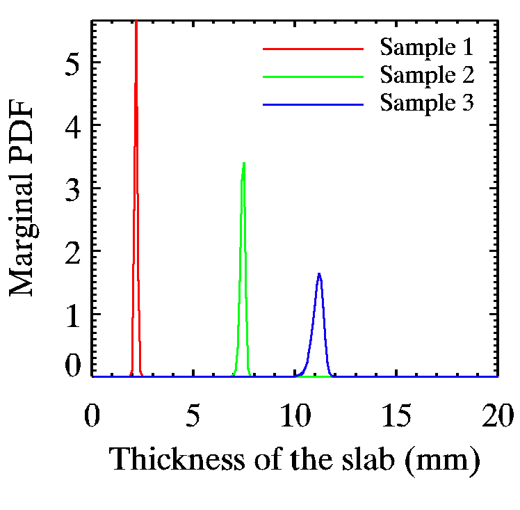
(a)
(b)

Figure 8: Marginal probability density functions a posteriori for (a) the thickness of the slab $\mathcal{P}\left\{p_{1}(i)\right\}$ and (b) the grain-size of the snow substrate $\mathcal{P}\left\{p_{2}(j)\right\}$ for the three samples, and for the geometries described in Figure 7. The functions are very sharp and very close to gaussian for the thickness of the slab (a), but are broad for the grain-size of the substrate (b). The thickness is well constrained by the inversion, whereas the grain-size of the substrate cannot be determined with high precision.

Figure 9: Results of the inversion and measures with error bars at $2\sigma$ for samples 1, 2 and 3, and for the 39 different geometries of measurement. The thicknesses retrieved and measured are compatible. The inversion points (in red) are sorted by incidence (3 values), and each incidence is then sorted by azimuth (13 values : 1 for emergence $0\text{\textdegree}$ and 6 for each $10\text{\textdegree\ and $20\text{\textdegree}$}$ emergences). The geometry seems to have an impact on the result for sample 1 and 2. The thickness estimated seems to increase with incidence, and decrease with azimuth. The geometrical effect seems to disappear for big thicknesses.

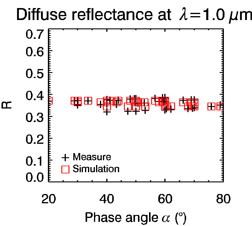
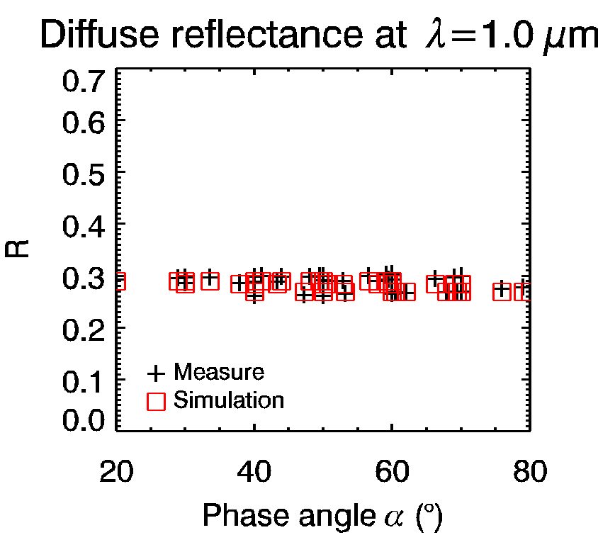
(a) Sample 1. Thickness : $1.42\pm 0.54mm$ (b) Sample 2. Thickness : $7.45\pm 0.84mm$ (c) Sample 3. Thickness : $12.51\pm 2.7mm$

Figure 10: Measured and simulated reflectance factor at $\lambda=1\,\mbox{$\mu$m}$ for (a) sample 1, (b) sample 2 and (c) sample 3. The simulation reproduces, if not perfectly, reasonably the geometrical behavior of the surfaces. The quality of the geometrical simulation seems to increase with the thickness of the slab. This is consistent with the isotropization effect of a slab, that will increase with the thickness.

(a) (b)

Figure 11: Marginal probability density functions a posteriori for (a) the thickness of the slab $\mathcal{P}\left\{p_{1}(i)\right\}$ and (b) the grain-size of the snow substrate $\mathcal{P}\left\{p_{2}(j)\right\}$ for the three sample thickness. The functions are very sharp and very close to gaussian for the thickness of the slab (a). The a posteriori uncertainties on the results are much smaller than the previous ones, because the dataset is bigger and thus more constraining. Still, these uncertainties are not fully reliable, as the model cannot reproduce perfectly within the a priori uncertainties the BRDF (see Figure 10). (b) The grainsize can be determined or the sample 1, and is consistent with the results on inversions of single spectra (see Figure LABEL:fig:Marginal_g). On the contrary, they cannot be inverted for sample 2 and 3, as the returned probability density function is close to a Dirac at the boundary of the definition range.

4.2 Diffuse

To reproduce diffuse reflectance we used the results obtained with the specular measurement and assumed that the roughness of the samples was not changing much between the experiments. The range of variations in roughness should be negligible in the spectral analysis. We simulated slabs over snow letting as free parameters the grain-size of the substrate and the thickness of the slab. Figure 7 represent examples of the best matches we obtained for the three measured samples at various geometries. We also represented the mismatch between the best fit and the observations. We find an agreement between the data and the model that is acceptable. Nevertheless, there seems to be a decrease of quality in the fits as the thickness increase. Figure 8 shows on the same plot an example of the marginal PDF for the three samples that are associated with the previous fits. Figure 8 for the thickness of the slab (a) and the grain-size of the snow substrate (b). The thickness is well constrained as the marginal probability density functions a posteriori are relatively sharp and very close to gaussian. On the contrary, the grain-size of the substrate seems to have a limited impact on the result since it is little constrained. The marginal PDF for the grain-size of the substrate are broad, and thus the a posteriori relative uncertainty on the result is very high. Unfortunately, we have no reliable measurement of the grain-size of the substrate, as it is evolving during the time of the measurements. The general trend of decreasing grainsize seems to be in agreement with eye’s impression.

Figure 9 show the measurements and the final result of the inversion of the thickness for the three samples, and for 39 measurement geometries independently. The data and the model are compatible. Still, the thickness of the sample 1 is slightly overestimated. This may reveal a sensitivity limit of the model. The thickness of sample 3 seems underestimated. This could be partly due to the duration of the measurement : the slab sublimates as the measure is being taken. Moreover, the specular measurements were performed on that sample increasing even more the duration of the experiment. The inversions points on Figure 9 are sorted by increasing incidence, and for each incidence, by increasing azimuth. There seems to have an influence of the geometry on the returned result : it is particularly clear for sample 2. The estimated thickness tend to increase with incidence and decrease with azimuth. This effect disappear for large thicknesses (sample 3). Figure 10 show the measure and the best match at the $\lambda=1.0\,\mbox{$\mu$m}$ wavelength, when conducting the inversion on the whole BRDF dataset for each sample. The relatively flat behavior of the radiation with the phase angle is reasonably well reproduced. The quality of the geometrical match increases with the thickness of the sample. This is consistent with the fact that a thicker slab will permit a stronger isotropization of the radiation. It is also consistent with the disappearance of the geometrical dependence on the estimation for large thicknesses noted on Figure 9. The values of thicknesses returned by the inversion are displayed on Figure 11a : they are also compatible with the data, and the results are close to the one given by independent inversions on each geometry (see Figures 8 and 9). The grainsizes returned, even if compatible with the independent inversion results, are at the boundary of the definition range of the parameter, for samples 2 and 3. This mean that the model cannot estimate this parameter correctly. Indeed, as displayed on Figure 11, the a posteriori marginal probability density functions for the samples 2 and 3 are very close to a Dirac at the lower limit of the domain. This mean that the model inversion process cannot fit a value for this parameter inside the definition domain that is fully satisfying. This suggest an evolution of the conditions of the experiment between the measure for the sample 1 and the others. The fact that the returned value is at the lower boundary of the grain-size range suggest the the actual grainsize of the snow is lower than this value. Unfortunately, such grain-size would contradict the fundamental hypothesis of geometrical optics assumed by the model. This results thus shall be interpreted as grain-sizes smaller than the limit of detection. This kind of very small grain-size could be produced during the experiments, by a small temperature difference between the slabs and the natural snow, resulting in the condensation of frost at the bottom of the slab layer.

[Discussion and conclusion]

The aim of this present work is to validate an approximate radiative transfer model developed in Andrieu et al. (2015) using several assumptions. The most debating one is the isotropization of the radiation when it reaches the substrate. We first validated qualitatively this assumption with snow and ice data. We then quantitatively tested and validated our method using a pure slab ice with various thickness and snow as a bottom condition. The thicknesses retrieved by the inversion are compatible with the measurements for every geometry, demonstrating the robustness of this method to retrieve the slab thickness from spectroscopy only. The result given by the inversion of the whole dataset is also compatible with the measurements.

We also validate the angular response of such slab in the specular lobe. Unfortunately, it was not possible to measure the micro-topography in detail to compare with the retrieved data. Nevertheless, we found a very good agreement between the simulation and the data. The average slope is compatible with a long wavelength slope at the scale of the sample, demonstrating that the micro-scale was not important in our case. This is probably due to the sharp slicing method used. In future work, an experimental validation of the specular lobe and roughness should be addressed.

The large uncertainties on the grain size inversion demonstrate that the bottom condition is less important than the slab for the radiation field at first order, as expected. Even at a thickness of $1.4\,\mbox{mm}$, since water ice is highly absorbent, the bottom layer is difficult to sense.

On figure 7, there seems to be a decrease in the quality of the fit when the slab thickness increase. We explain it by the order in which the experiments were conducted. Indeed, the first measurement was of the thinnest slab and the last on the thickest. In the meantime, the snow substrate was sublimating. The errors in the fits could be due to the increasing contamination in the substrate. The natural snow cannot be perfectly pure : as it sublimates during the measurements, the contribution of the contaminants become stronger and stronger. These contaminant are not known, and not taken into account in the model. A way to avoid this problem could be to set the slab ice on top of a non volatile granular material, such as dry mineral sand, which optical constants are known or can be determined. However this would not solve another problem that is the re-condensation of water into frost between the granular substrate and the slab.

The comparison of the a posteriori uncertainties on the thickness of the slab and the grain-size of the snow substrate illustrate the fact that those uncertainties depend both on the constraint brought by the model itself and the uncertainty introduced in the measurement, that only the bayesian approach can handle. The use of bayesian formalism, is thus very powerful in comparison with traditional minimization techniques.

We propose here an fast and innovative inversion method aiming at massive inversion, for instance for remote sensing spectro-imaging data, that enables to accurately estimate the uncertainties on the model’s parameters. As an example, the look-up table used for this project were computed in $\sim 150\,\mbox{s}$ for the roughness study (1763 wavelengths sampled, 30933 spectra), and $\sim 2.5\,\mbox{h}$ for the thickness and grainsize study (33,186 wavelengths sampled, 666,315 spectra). The inversion itself were performed in less than one tenth of a second for specular lobe and independent spectral inversions, and $2\,\mbox{s}$ for BRDF-as-a-whole inversions. Every calculation was computed on one $4\,\mbox{GB}$ RAM Intel CPU. It has to be noted that once the lookup table has been created, an unlimited number of inversion can be conducted. The model is fast and the inversion is highly parallel and thus adapted to the study of the compact ice covered surfaces of the Solar system. For inversion over very large databases, the code has been adapted to GPU paralellization. It is also possible to increase de speed of the calculation of the look-up tables by doing a multi-CPU computing.

References

- Andrieu et al. (2015) Andrieu, F., Douté, S., Schmidt, F., and Schmitt, B.: Radiative transfer model for contaminated rough slabs, ArXiv e-prints, 2015.
- Appéré et al. (2011) Appéré, T., Schmitt, B., Langevin, Y., Douté, S., Pommerol, A., Forget, F., Spiga, A., Gondet, B., and Bibring, J.-P.: Winter and spring evolution of northern seasonal deposits on Mars from OMEGA on Mars Express, Journal of Geophysical Research: Planets, 116, n/a–n/a, 10.1029/2010JE003762, URL http://dx.doi.org/10.1029/2010JE003762, 2011.
- Brissaud et al. (2004) Brissaud, O., Schmitt, B., Bonnefoy, N., Douté, S., Rabou, P., Grundy, W., and Fily, M.: Spectrogonio radiometer for the study of the bidirectional reflectance and polarization functions of planetary surfaces. 1. Design and tests, Appl. Opt., 43, 1926–1937, URL http://ao.osa.org/abstract.cfm?URI=ao-43-9-1926, 2004.
- Carmagnola et al. (2013) Carmagnola, C. M., Domine, F., Dumont, M., Wright, P., Strellis, B., Bergin, M., Dibb, J., Picard, G., Libois, Q., Arnaud, L., and Morin, S.: Snow spectral albedo at Summit, Greenland: measurements and numerical simulations based on physical and chemical properties of the snowpack, The Cryosphere, 7, 1139–1160, 10.5194/tc-7-1139-2013, URL http://www.the-cryosphere.net/7/1139/2013/, 2013.
- Chandrasekhar (1960) Chandrasekhar, S.: Radiative transfer, Dover, 1960.
- Douté and Schmitt (1998) Douté, S. and Schmitt, B.: A multilayer bidirectional reflectance model for the analysis of planetary surface hyperspectral images at visible and near-infrared wavelengths, J. Geophys. Res., 103, 31 367–31 389, URL http://dx.doi.org/10.1029/98JE01894, 1998.
- Dozier et al. (2009) Dozier, J., Green, R. O., Nolin, A. W., and Painter, T. H.: Interpretation of snow properties from imaging spectrometry, Remote Sensing of Environment, 113, Supplement 1, S25–S37, URL http://www.sciencedirect.com/science/article/pii/S0034425709000777, 2009.
- Dumont et al. (2010) Dumont, M., Brissaud, O., Picard, G., Schmitt, B., Gallet, J.-C., and Arnaud, Y.: High-accuracy measurements of snow Bidirectional Reflectance Distribution Function at visible and NIR wavelengths ‚Äì comparison with modelling results, Atmos. Chem. Phys., 10, 2507–2520, URL http://www.atmos-chem-phys.net/10/2507/2010/, 2010.
- Dumont et al. (2014) Dumont, M., Brun, E., Picard, G., Michou, M., Libois, Q., Petit, J.-R., Geyer, M., Morin, S., and Josse, B.: Contribution of light-absorbing impurities in snow to Greenland/’s darkening since 2009, Nature Geosci, 7, 509–512, URL http://dx.doi.org/10.1038/ngeo2180, 2014.
- Eluszkiewicz and Moncet (2003) Eluszkiewicz, J. and Moncet, J.-L.: A coupled microphysical/radiative transfer model of albedo and emissivity of planetary surfaces covered by volatile ices, Icarus, 166, 375–384, URL http://www.sciencedirect.com/science/article/pii/S0019103503002628, 2003.
- Eluszkiewicz et al. (2005) Eluszkiewicz, J., Moncet, J.-L., Titus, T. N., and Hansen, G. B.: A microphysically-based approach to modeling emissivity and albedo of the martian seasonal caps, Icarus, 174, 524–534, URL http://www.sciencedirect.com/science/article/pii/S0019103504003598, 2005.
- Hapke (1981) Hapke, B.: Bidirectional reflectance spectroscopy: 1. Theory, J. Geophys. Res., 86, 3039–3054, URL http://dx.doi.org/10.1029/JB086iB04p03039, 1981.
- Hapke (1984) Hapke, B.: Bidirectional reflectance spectroscopy: 3. Correction for macroscopic roughness, Icarus, 59, 41–59, URL http://www.sciencedirect.com/science/article/pii/001910358490054X, 1984.
- Kieffer and Titus (2001) Kieffer, H. H. and Titus, T. N.: TES Mapping of Mars’ North Seasonal Cap, Icarus, 154, 162–180, URL http://www.sciencedirect.com/science/article/pii/S0019103501966709, 2001.
- Leighton and Murray (1966) Leighton, R. B. and Murray, B. C.: Behavior of Carbon Dioxide and Other Volatiles on Mars, Science, 153, 136–144, URL http://www.sciencemag.org/content/153/3732/136.abstract, 1966.
- Lhermitte et al. (2014) Lhermitte, S., Abermann, J., and Kinnard, C.: Albedo over rough snow and ice surfaces, The Cryosphere, 8, 1069–1086, 10.5194/tc-8-1069-2014, URL http://www.the-cryosphere.net/8/1069/2014/, 2014.
- Mary et al. (2013) Mary, A., Dumont, M., Dedieu, J.-P., Durand, Y., Sirguey, P., Milhem, H., Mestre, O., Negi, H. S., Kokhanovsky, A. A., Lafaysse, M., and Morin, S.: Intercomparison of retrieval algorithms for the specific surface area of snow from near-infrared satellite data in mountainous terrain, and comparison with the output of a semi-distributed snowpack model, The Cryosphere, 7, 741–761, URL http://www.the-cryosphere.net/7/741/2013/, 2013.
- Mosegaard and Tarantola (1995) Mosegaard, K. and Tarantola, A.: Monte Carlo sampling of solutions to inverse problems, J. Geophys. Res., 100, 12 431–12 447, URL http://dx.doi.org/10.1029/94JB03097, 1995.
- Negi and Kokhanovsky (2011) Negi, H. S. and Kokhanovsky, A.: Retrieval of snow albedo and grain size using reflectance measurements in Himalayan basin, The Cryosphere, 5, 203–217, 10.5194/tc-5-203-2011, URL http://www.the-cryosphere.net/5/203/2011/, 2011.
- Painter and Dozier (2004) Painter, T. H. and Dozier, J.: The effect of anisotropic reflectance on imaging spectroscopy of snow properties, Remote Sensing of Environment, 89, 409–422, URL http://www.sciencedirect.com/science/article/pii/S0034425703002578, 2004.
- Picard et al. (2009) Picard, G., Arnaud, L., Domine, F., and Fily, M.: Determining snow specific surface area from near-infrared reflectance measurements: Numerical study of the influence of grain shape, Cold Regions Science and Technology, 56, 10–17, URL http://www.sciencedirect.com/science/article/pii/S0165232X08001602, 2009.
- Pilorget et al. (2013) Pilorget, C., Vincendon, M., and Poulet, F.: A radiative transfer model to simulate light scattering in a compact granular medium using a Monte Carlo approach: Validation and first applications, J. Geophys. Res. Planets, 118, 2488–2501, URL http://dx.doi.org/10.1002/2013JE004465, 2013.
- Schmitt et al. (1998) Schmitt, B., Quirico, E., Trotta, F., and Grundy, W. M.: Optical Properties of Ices from UV to Infrared, in: Solar System Ices, edited by Schmitt, B., de Bergh, C., and Festou, M., vol. 227 of Astrophysics and Space Science Library, pp. 199–240, Kluwer, 1998.
- Shkuratov et al. (1999) Shkuratov, Y., Starukhina, L., Hoffmann, H., and Arnold, G.: A Model of Spectral Albedo of Particulate Surfaces: Implications for Optical Properties of the Moon, Icarus, 137, 235–246, 10.1006/icar.1998.6035, URL http://www.sciencedirect.com/science/article/pii/S0019103598960353, 1999.
- Stamnes et al. (1988) Stamnes, K., Tsay, S.-C., Wiscombe, W., and Jayaweera, K.: Numerically stable algorithm for discrete-ordinate-method radiative transfer in multiple scattering and emitting layered media, Appl. Opt., 27, 2502–2509, URL http://ao.osa.org/abstract.cfm?URI=ao-27-12-2502, 1988.
- Tarantola (1982) Tarantola, A.: Inverse problems - quest for information, 1982.
- Warren and Brandt (2008) Warren, S. G. and Brandt, R. E.: Optical constants of ice from the ultraviolet to the microwave: A revised compilation, J. Geophys. Res., 113, D14 220–, URL http://dx.doi.org/10.1029/2007JD009744, 2008.
- Zent et al. (1989) Zent, A. P., McKay, C. P., Pollack, J. B., and Cruikshank, D. P.: Grain metamorphism in polar nitrogen ice on Triton, Geophysical Research Letters, 16, 965–968, 10.1029/GL016i008p00965, URL http://dx.doi.org/10.1029/GL016i008p00965, 1989.