Fluctuation relations for anomalous dynamics generated by time-fractional Fokker-Planck equations

Abstract

Anomalous dynamics characterized by non-Gaussian probability distributions (PDFs) and/or temporal long-range correlations can cause subtle modifications of conventional fluctuation relations. As prototypes we study three variants of a generic time-fractional Fokker-Planck equation with constant force. Type A generates superdiffusion, type B subdiffusion and type C both super- and subdiffusion depending on parameter variation. Furthermore type C obeys a fluctuation-dissipation relation whereas A and B do not. We calculate analytically the position PDFs for all three cases and explore numerically their strongly non-Gaussian shapes. While for type C we obtain the conventional transient work fluctuation relation, type A and type B both yield deviations by featuring a coefficient that depends on time and by a nonlinear dependence on the work. We discuss possible applications of these types of dynamics and fluctuation relations to experiments.

1 Introduction

Understanding fluctuations far from equilibrium defines a key topic of nonequilibrium statistical physics. A new line of activities started about three decades ago by discovering different forms of fluctuation relations (FRs) which generalize fundamental laws of thermodynamics to small systems in nonequilibrium; see Refs. [1, 2, 3, 4, 5, 6, 7, 8] for reviews and further references therein. More recently these laws got unified by over-arching schemes, most notably the deterministic dissipation function approach by Evans and coworkers [1], and by stochastic thermodynamics [9, 10, 7, 11]. The latter theory starts from defining entropy production on the level of individual trajectories in stochastic models such as Langevin and master equations. Given that stochastic thermodynamics is based on rather simple Markov models one may ask to which extent FRs derived from it are reproduced if the dynamics is more complicated. In our paper we address this problem by testing FRs for stochastic dynamics that is anomalous due to non-Markovian dynamical correlations and/or strongly non-Gaussian PDFs.

Anomalous dynamics has been observed in many experiments and is widely studied by the theory of anomalous stochastic processes [12, 13, 14, 15, 16, 17]. A characteristic property of anomalous dynamics is that the mean square displacement (MSD) grows nonlinearly in time yielding anomalous diffusion in the long time limit [15]. In contrast, Markovian dynamics like Brownian motion generates a MSD that increases linearly for long times. If the MSD grows faster than linear one speaks of superdiffusion, if it grows slower than linear one obtains subdiffusion. There are many different ways to model anomalous stochastic dynamics such as continuous time random walks (CTRW) [18, 19, 20, 12], generalized Langevin equations [21, 13, 22, 23], Lévy flights and walks [24, 17], fractional diffusion equations [16], scaled Brownian motion [25, 26] and heterogeneous diffusion processes [27], to name a few.

The study of FRs for anomalous stochastic processes appears to be rather at the beginning: Crooks and Jarzynski work relations as well as transient and steady state fluctuation theorems have been confirmed for non-Markovian Gaussian dynamics modelled by generalized Langevin equations with memory kernels, given specific conditions are fulfilled [28, 29, 30, 31]. These results have been reproduced and generalized by a stochastic thermodynamics approach [32]. For non-Gaussian PDFs generated by Langevin equations with non-Gaussian noise, such as Lévy noise or Poissonian shot noise, violations of conventional steady state and transient FRs have been reported [33, 34, 35, 36, 37, 38]. For a CTRW model with a power law waiting time distribution it was found that the steady state FRs may or may not hold depending on the exponent of the waiting time distribution [39]. Computer simulations of glassy dynamics exhibiting anomalous diffusion also showed violations of transient fluctuation relations [40, 41]. In [42, 43, 44] several of the above types of stochastic dynamics including fractional Fokker-Planck equations were considered. It was found that the validity of fluctuation-dissipation relations [45] for a given anomalous stochastic process plays a crucial role for the validity or violation of conventional FRs.

In this article we test transient fluctuation relations (TFRs) for a class of anomalous stochastic processes that so far has not been in the focus of investigations, which are time-fractional Fokker-Planck equations (FFPEs). Such equations model the emergence of non-Gaussian PDFs by using power law memory kernels via time-fractional derivatives [46]. They need to be distinguished from equations modeling correlations in space via space-fractional derivatives as they naturally arise, e.g., for generating Lévy flights [12, 42]. FFPE can be derived from stochastic equations of motion either by CTRWs [12, 16] or by subordinated Langevin dynamics [47]. Quite a variety of them have been studied in the literature, both from a purely theoretical point of view and with respect to applications to experiments: Prominent examples are fractional Klein-Kramers equations that were used to analyse biological cell migration data [48, 49, 50]. Another type was designed to model the dynamics of tracer particles in random environments [51]. Closely related time-fractional diffusion equations [21, 52, 12] have been used to model a variety of different processes, from diffusion in crowded cellular environments [53, 15] to geophysical and environmental systems [14]. They have also been derived for weakly chaotic dynamical systems [54, 55]. A bifractional diffusion equation famously reproduced the spreading of dollar bills in the United States [56].

Our paper is structured as follows: In Section 2 we discuss three types of FFPEs which differ from each other in terms of their anomalous diffusive properties, and by whether or not they fulfill fluctuation-dissipation relations. We solve these models for their position PDFs and study their properties both analytically and numerically. In Section 3 we test the (work) TFR for our three models by analytical asymptotic expansions and by numerically plotting the results. We conclude with a summary and an outlook towards physical applications in Section 4.

2 Time-fractional Fokker-Planck equations

This section introduces to three different types of FFPEs: We first outline how starting from stochastic dynamics a FFPE generating superdiffusion can be constructed in the form of an overdamped Langevin equation with correlated noise. Our argument illustrates how a time-fractional derivative naturally emerges from modelling power law time correlation decay. The other two types of FFPEs that we consider have already been derived in the literature from CTRW theory and are either subdiffusive or exhibit a transition from sub- to superdiffusion under parameter variation. We analytically calculate the first and second moments for all three models, which enables us to check for the validity of the fluctuation-dissipation relation of the first kind (FDR1). We also comment on the Galilean invariance of our models. We then analytically calculate the position PDFs of all FFPEs and study the solutions numerically by plotting the results.

2.1 Constructing a superdiffusive fractional Fokker-Planck equation

The study of an overdamped Langevin equation for the position $x(t)$ of a particle on the line driven by a correlated stochastic process and an external force allows to gain insight into the origin of a superdiffusive FFPE. Our Langevin equation of interest is given by

$$\frac{dx}{dt}=\frac{F_{0}}{m\gamma_{\alpha}}+v(t),$$ (1)

where $F_{0}$ denotes a constant external force, $\gamma_{\alpha}$ a friction coefficient and $m$ the mass of the particle. We assume that $v(t)$ is a stationary correlated stochastic process with zero mean $\langle v(t)\rangle=0$ and a power-law correlation function

$$\langle v(t)\;v(t_{1})\rangle=\frac{K_{\alpha}}{\Gamma(\alpha-1)}\frac{1}{|t-t_{1}|^{2-\alpha}}$$ (2)

with $1<\alpha<2$, gamma function $\Gamma$ and generalized diffusion coefficient $K_{\alpha}$. Note that we do not further specify the noise. Following the pseudo-Liouville hybrid approach of Balescu [57, 58] (see A) one obtains the following exact result in Eq. 46 for the PDF $f(x,t)$:

$$\left(\frac{\partial}{\partial t}+v_{0}\frac{\partial}{\partial x}\right)f(x,t)=\frac{\partial^{2}}{\partial x^{2}}\int\limits_{0}^{t}dt_{1}\;\Big{\langle}v(t)v(t_{1})\;f\left(x-\Delta(t,t_{1}),t_{1}\right)\Big{\rangle}$$ (3)

with $v_{0}=F_{0}/(m\gamma_{\alpha})$ and $\Delta(t,t_{1})=v_{0}(t-t_{1})+\int\limits_{t_{1}}^{t}dt_{2}\;v(t_{2})$. This exact equation is non-local in time (i.e. non-Markovian) and non-local in space. We now make a local-in-space approximation by neglecting the term of the fluctuating displacement $\Delta(t,t_{1})$ on the right hand side of the probability density $f$. Such an approximation seems to be reasonable in the long time and large space asymptotic limit if the drift and velocity fluctuations are weak enough. This assumption results in the following non-Markovian Fokker-Planck equation:

$$\left(\frac{\partial}{\partial t}+v_{0}\frac{\partial}{\partial x}\right)f(x,t)=\frac{\partial^{2}}{\partial x^{2}}\int\limits_{0}^{t}dt_{1}\;\langle v(t)v(t_{1})\rangle\;f(x,t_{1})\>.$$ (4)

Insertion of the correlation function of velocities Eq. 2 into Eq. 4 leads to

$$\left(\frac{\partial}{\partial t}+v_{0}\frac{\partial}{\partial x}\right)f(x,t)=\frac{\partial^{2}}{\partial x^{2}}\frac{K_{\alpha}}{\Gamma(\alpha-1)}\int\limits_{0}^{t}dt_{1}\;(t-t_{1})^{\alpha-2}\;f(x,t_{1})\>.$$ (5)

The integral on the right hand side matches to the Riemann-Liouville (RL) fractional integral of order $\mu$ given by [59]

$$J_{t}^{\mu}\;g(t)\equiv D_{t}^{-\mu}g(t)=\frac{1}{\Gamma(\mu)}\int\limits_{0}^{t}d\tau\;(t-\tau)^{\mu-1}\;g(\tau)$$ (6)

with $\mu>0$ and $\mu=\alpha-1$ for Eq. 5. We also introduce the definition of the RL fractional derivative of positive order

$$D_{t}^{\mu}\;g(t)=\frac{d^{n}}{dt^{n}}\;J_{t}^{n-\mu}\;g(t)$$ (7)

with $\mu>0\>,\>n=\left[\mu\right]+1$, where $\left[\ldots\right]$ refers to the integer part of the given number. Applying Eq. 6 to Eq. 5 gives us our first type of FFPE that we denote as

$$\mbox{type A:}\;\;\;\frac{\partial f_{A}(x,t)}{\partial t}=-\frac{\partial}{\partial x}\left[v_{0}-K_{\alpha}D_{t}^{1-\alpha}\frac{\partial}{\partial x}\right]f_{A}(x,t)\>,\>1<\alpha<2\>.$$ (8)

To show the relation of this equation with previous works we put $v_{0}=0$. Then it can be written as

$$\frac{\partial^{2}}{\partial t^{2}}f(x,t)=K_{\alpha}\;\frac{\partial^{2}}{\partial x^{2}}\;D_{t}^{2-\alpha}f(x,t)\>,1<\alpha<2\>.$$ (9)

This equation was called a fractional wave equation in the seminal paper of Schneider and Wyss [52] and has also been derived for a long-range correlated dichotomous stochastic process [60] from a fractional Klein-Kramers equation [48] and from a generalised Chapman-Kolmogorov equation [61]. The solution of this equation has been studied in detail in [62] where it was called a fractional kinetic equation for sub-ballistic superdiffusion. The equivalent form of this equation using the Caputo fractional derivative was investigated in [63].

Our presentation above illustrates how a FFPE can be derived from a Langevin equation with power-law decay in the velocity correlation function. It furthermore demonstrates that a fractional derivative provides the natural mathematical formulation to model equations containing power law memory kernels.

2.2 Definition and properties of fractional Fokker-Planck equations

In addition to type A FFPE Eq. 8 we consider two further types of FFPEs. Both have been derived from CTRW theory [18, 19, 20, 12]. Note that the underlying stochastic dynamics and the derivation of these two FFPEs are very different from what we presented for type A above. Indeed, both type B and type C are essentially (almost) Markovian models, in contrast to type A. Our two new FFPEs describe subdiffusion under the influence of a constant external force and naturally appear in physical systems where diffusion is slowed down by deep traps [12, 20, 64]. The difference between these two types arises from the position of the fractional RL derivative with respect to the diffusive and drift part of the equations and the range of the anomaly parameter $\alpha$. Our second FFPE is defined as

$$\mbox{type B:}\;\;\;\frac{\partial f_{B}(x,t)}{\partial t}=-\frac{\partial}{\partial x}\left[v_{0}-K_{\alpha}D_{t}^{1-\alpha}\frac{\partial}{\partial x}\right]f_{B}(x,t).$$ (10)

For type C FFPE the RL fractional derivative is also included in the drift term:

$$\mbox{type C:}\;\;\;\frac{\partial f_{C}(x,t)}{\partial t}=-\frac{\partial}{\partial x}\left[A_{\alpha}v_{0}D_{t}^{1-\alpha}-K_{\alpha}D_{t}^{1-\alpha}\frac{\partial}{\partial x}\right]f_{C}(x,t),$$ (11)

where $A_{\alpha}$ has a dimension of time to the power of $1-\alpha$. Note that type B and type C FFPEs are defined for $0<\alpha<1$ whereas for type A FFPE $\alpha$ is in the range $1<\alpha<2$. For all three FFPEs we use the initial condition $f_{A,B,C}(x,t=0)=\delta(x)$. By means of Fourier and Laplace transforms

$$\hat{f}(k)=\int\limits_{-\infty}^{\infty}dxe^{ikx}f(x),\;\;\;\;\;\;\tilde{f}(s)=\int\limits_{0}^{\infty}dte^{-st}f(t)$$ (12)

a solution of Eqs. 8, 10 and 11 can be obtained in Fourier-Laplace space as

$$\hat{\tilde{f}}_{A,B}(k,s)=\frac{1}{s+v_{0}ik+K_{\alpha}k^{2}s^{1-\alpha}},$$ (13)

$$\hat{\tilde{f}}_{C}(k,s)=\frac{1}{s+A_{\alpha}v_{0}iks^{1-\alpha}+K_{\alpha}k^{2}s^{1-\alpha}},$$ (14)

where the fractional derivative $D^{1-\alpha}_{t}f(t)$ transforms to $s^{1-\alpha}\tilde{f}(s)$. The solutions of type A and type B FFPE only differ in the range of $\alpha$ as defined above. The representation in Fourier-Laplace space allows the calculation of moments by differentiation with respect to $k$:

$$\langle x^{n}(t)\rangle={\cal L}^{-1}\left\{(i)^{n}\left.\frac{\partial^{n}\hat{\tilde{f}}(k,s)}{\partial k^{n}}\right|_{k=0}\right\}.$$ (15)

After Laplace inversion one obtains the first two moments and the central second moment for $\delta x=x-\langle x\rangle$ of type C FFPE defined in Eq. 11 [20]

$$\langle x\rangle_{C} = \frac{A_{\alpha}v_{0}t^{\alpha}}{\Gamma(\alpha+1)},$$ (16)

$$\langle x^{2}\rangle_{C} = \frac{2K_{\alpha}t^{\alpha}}{\Gamma(\alpha+1)}+\frac{2A_{\alpha}^{2}v_{0}^{2}t^{2\alpha}}{\Gamma(2\alpha+1)},$$ (17)

$$\langle(\delta x)^{2}\rangle_{C} = \frac{2K_{\alpha}t^{\alpha}}{\Gamma(\alpha+1)}+A_{\alpha}^{2}v_{0}^{2}t^{2\alpha}\;\left[\frac{2}{\Gamma(2\alpha+1)}-\frac{1}{\Gamma(\alpha+1)^{2}}\right].$$ (18)

These results show that the FDR1 [45, 43] $\langle x(t)\rangle_{C}\sim\langle x^{2}(t)\rangle^{v_{0}=0}_{C}$ is valid for type C. Interestingly the external force influences the second central moment $\sim v_{0}^{2}t^{2\alpha}$. Technically this is due to the coupling term $v_{0}iks^{1-\alpha}$ in the Laplace-Fourier representation of Eq. 14. The first moment increases sublinearly despite the constant external force. This can be interpreted as a partial sticking effect of particles [65]. By contrast, the second central moment shows a crossover from $\sim t^{\alpha}$ to $\sim t^{2\alpha}$. Thus, for $v_{0}\neq 0$ type C switches from a subdiffusive behavior of the second central moment for $0<\alpha<1/2$ to a superdiffusive behavior for $1/2<\alpha<1$ [12].

Analogously, the moments of type A and type B FFPEs of Eq. 8 and Eq. 10 are obtained as [20]

$$\langle x\rangle_{A,B} = v_{0}t,$$ (19)

$$\langle x^{2}\rangle_{A,B} = \frac{2K_{\alpha}t^{\alpha}}{\Gamma(\alpha+1)}+v_{0}^{2}t^{2},$$ (20)

$$\langle(\delta x)^{2}\rangle_{A,B} = \frac{2K_{\alpha}t^{\alpha}}{\Gamma(\alpha+1)}.$$ (21)

In both cases the first moment only depends on $v_{0}$ and increases linearly in time. The second central moment shows a superdiffusive and subdiffusive increase $\sim t^{\alpha}$ for type A and type B FFPE, respectively. In contrast to type C FFPE, the second moment of type A and type B FFPEs is without any coupling to $v_{0}$. In addition, type A and type B FFPEs break FDR1 between the first $\langle x(t)\rangle_{A,B}$ and the second moment $\langle x^{2}(t)\rangle^{v_{0}=0}_{A,B}$. In both cases this is what one should expect according to the definition of both models: Type A is based on the Langevin equation 1 where the fluctuation-dissipation relation of the second kind (FDR2) is broken by construction. Note that FDR2 establishes a relation between the noise and the friction [45]. The breaking of FDR2 suggests a breaking of FDR1 as was shown for Gaussian stochastic processes in [43]. For type B the fractional derivative acts only on the diffusion term in Eq. 10 thus breaking FDR1 while for type C it acts simultaneously on both the drift and the diffusion terms in Eq. 11 hence preserving FDR1.

A second difference between these FFPEs consists in their behavior under Galilean transformation. With $X=x-v_{0}t$ and $T=t$ the PDF $f(x,t)$ is transformed to $\Omega(X,T)$. The coupling of the fractional RL derivative to the $v_{0}$ drift term of type C FFPE in Eq. 11 breaks Galilean invariance. However, type A and B FFPE of Eq. 8 and Eq. 10 fulfill Galilean invariance in the long time and large space limit [20, 12, 66], where they can be written as

$$\frac{\partial\Omega_{A,B}(X,T)}{\partial T}=K_{\alpha}D^{1-\alpha}_{T}\frac{\partial^{2}\Omega_{A,B}(X,T)}{\partial X^{2}}\>.\\$$ (22)

This means that in this limit breaking or preserving FDR1 corresponds to preserving respectively breaking Galilean invariance in the case of these FFPEs. This property will be exploited in the next subsection where we discuss analytical and numerical solutions of our three types of FFPEs.

2.3 Analytical solution of time-fractional Fokker-Planck equations

Type C FFPE:

Fourier inversion [42] leads to the solution of type C FFPE in $(x,s)$ space:

$$\tilde{f}_{C}(x,s)=\frac{s^{\alpha-1}}{\sqrt{A_{\alpha}^{2}v_{0}^{2}+4K_{\alpha}s^{\alpha}}}\exp\left(\frac{A_{\alpha}v_{0}x}{2K_{\alpha}}-|x|\frac{\sqrt{A_{\alpha}^{2}v_{0}^{2}+4K_{\alpha}s^{\alpha}}}{2K_{\alpha}}\right).$$ (23)

In this case, a solution in $(x,t)$ space can be given as a superposition of the $\alpha=1$ Gaussian solution with a Lévy kernel [67, 12]. However, for numerical analysis we apply a direct numerical Laplace inversion of Eq. 23.

Type A and B FFPE:

Analogously to Eq. 23 the solutions of type A and type B FFPEs can be calculated in $(x,s)$ space with $A_{\alpha}v_{0}\rightarrow v_{0}s^{\alpha-1}$ to

$$\tilde{f}_{A,B}(x,s)=\frac{s^{\alpha-1}}{\sqrt{v_{0}^{2}s^{2\alpha-2}+4K_{\alpha}s^{\alpha}}}\exp\left(\frac{v_{0}s^{\alpha-1}x}{2K_{\alpha}}-|x|\frac{\sqrt{v_{0}^{2}s^{2\alpha-2}+4K_{\alpha}s^{\alpha}}}{2K_{\alpha}}\right).$$ (24)

As the FFPEs of type A and type B are Galilean invariant in the long time and large space limit, the solution for $v_{0}=0$ allows the exact calculation of the PDFs with drift $v_{0}$ in this limit [20, 12], which becomes approximate otherwise [66]. The solution to Eq. 22 is well-known [12] and is given using a Fox $H$-function (see B for definitions). Thus, applying Galilean transformation and replacing $x$ with $x-v_{0}t$ gives solutions of type A and type B FFPEs in $(x,t)$ space as

$$f_{A,B}(x,t)=\frac{1}{\sqrt{4K_{\alpha}t^{\alpha}}}\;H^{10}_{11}\left[\frac{|x-v_{0}t|}{\sqrt{K_{\alpha}t^{\alpha}}}\left|\begin{matrix}\displaystyle(1-\alpha/2,\alpha/2)\\ (0,1)\end{matrix}\right.\right].$$ (25)

These approximate solutions in terms of shifted Fox functions are the basis for our further analysis of type A and B FFPEs.

2.4 Numerical analysis of time-fractional Fokker-Planck equations

Numerical methods are required to study the analytical results given in form of Fox $H$-functions of type A and type B FFPE and in Laplace space for type C FFPE.

Type A and type B FFPE:

The series expansion of the solution $f_{A,B}(x,t)$ of Eq. 25 as given by Eq. 49 is used for numerical evaluations,

$$f_{A,B}(x,t)=\frac{1}{\sqrt{4K_{\alpha}t^{\alpha}}}\sum_{j=0}^{\infty}\frac{(-1)^{j}}{j!\Gamma(1-\alpha(j+1)/2)}\left(\frac{(x-v_{0}t)^{2}}{K_{\alpha}t^{\alpha}}\right)^{j/2}$$ (26)

with $1<\alpha<2$ for type A FFPE and $0<\alpha<1$ for type B FFPE. The series is evaluated with multiple-precision arithmetic.

Type C FFPE:

Direct numerical Laplace inversion is applied to Eq. 23 to obtain the probability density function $f_{C}(x,t)$. Here we use a multiple-precision algorithm for the Laplace inversion based on Talbot’s method [68, 69].

Typical behavior in space and time:

Fig. 1 shows the time development of the solutions $f(x,t)$ of the three FFPE types for different times $t=1,2,4,8$. Parameters were selected as $A_{\alpha}v_{0}=1$ and $K_{\alpha}=1$, the anomaly index $\alpha$ was chosen from $\alpha\in(0.4,0.6...1.6)$. The first row shows the Gaussian limit $\alpha\rightarrow 1$ for all three types. In this normal diffusive case the PDF is spreading with $\sqrt{2K_{1}t}$ and its center is moving according to $v_{0}t$. The PDFs of type A (left column) and type B FFPE (middle column) preserve this constant drift for $\alpha\neq 1$. However, the shapes of the PDFs of both models immediately change profoundly showing characteristically different types of non-Gaussian behavior: For type A the PDFs spread superdiffusively with the variance of Eq. 21 by exhibiting a double-peaked structure with a dip in the middle. Qualitatively, the highly characteristic double-peak structure is explained in [58]: The propagator of type A decays asymptotically faster than the Gaussian, cf. Eq. 51. However, since two maxima move away from the origin in the opposite directions, superdiffusion is possible in spite of the thin tail of the propagator; see also Eq. 9 [62]. Note that there are cusp singularities in all three models for $\alpha\neq 1$, in contrast to the smooth behavior of the Gaussian PDF shown in the top row. In the Galilean invariant cases A and B the propagators are symmetric with respect to their cusps, which are translated with velocity $v_{0}=1$, as it should be. For the Galilean non-invariant model C the propagator is asymmetric with respect to its cusp, which stays fixed at the origin [12].

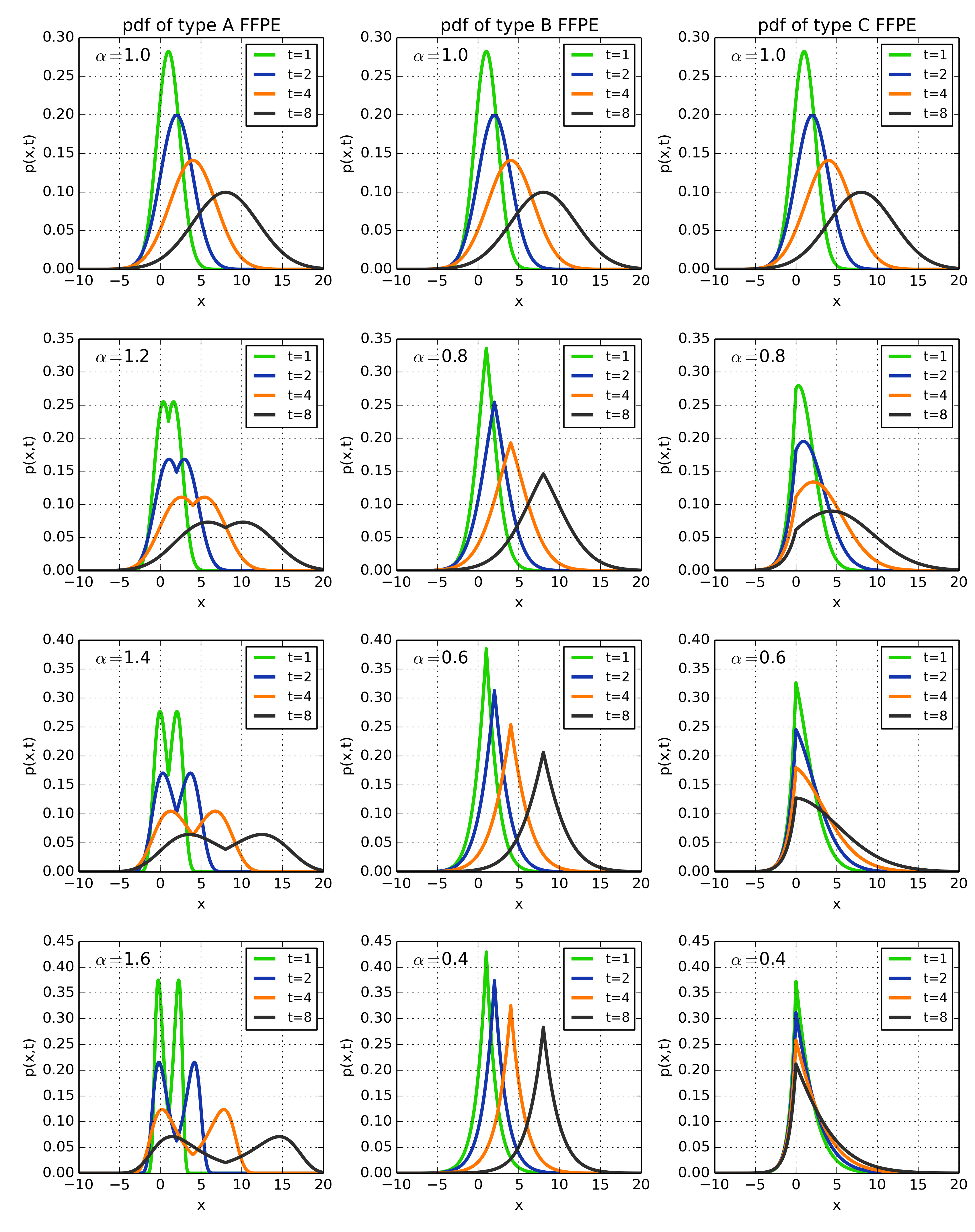
Figure 1: Time development of PDFs for type A FFPE (left column), type B FFPE (middle column) and type C FFPE (right column) for different values of $\alpha$ (rows) and time points $t=1,2,4,8$. Parameters were selected as $K_{\alpha}=1$, $v_{0}=1$ and $A_{\alpha}v_{0}=1$. Whereas superdiffusive type A FFPE (left column) and subdiffusive type B FFPE (middle column) show a drift and spreading of the PDFs with typical non-Gaussian structures for $\alpha\neq 1$, type C FFPE (right column) displays a spreading of the PDFs together with stickiness to the origin.

3 Work fluctuation relations for fractional Fokker-Planck equations

3.1 Definition of fluctuation relations

Using the results of the previous section, we now study the probability distribution $p(W,t)$ of the mechanical work $W=-F_{0}\;x$ generated by the constant external field $F_{0}$. For a constant field the probability distribution of work $p(W,t)$ is related to the probability distribution $f(x,t)$ of positions by the simple scaling transformation

$$p(W,t)=\frac{1}{F_{0}}f\left(\frac{W}{F_{0}},t\right).$$ (27)

It is the main aim of this work to study the TFR of the work PDFs defined by the logarithmic fluctuation ratio

$${\mathsf{R}}(W,t):=\log\frac{p(W,t)}{p(-W,t)}$$ (28)

for the three types of FFPEs. All three FFPE types reduce to a normal Gaussian process with drift for $\alpha\rightarrow 1$. For a Gaussian PDF the ratio ${\mathsf{R}}$ is trivially given by the ratio of the first and second central moment, i.e. $2\langle W\rangle/\langle\delta W^{2}\rangle$ [43]. Thus one obtains a normal or conventional fluctuation relation for $\alpha=1$,

$${\mathsf{R}}(W,t)\left|{}_{\alpha=1}\right.=\frac{v_{0}}{F_{0}K_{1}}\;W=W/(k_{B}T).$$ (29)

with a linear increase in $W$ that is independent of time as it has been found for a large class of systems [1, 2, 3, 6, 7, 8]. The last expression has been obtained by using the Einstein relation $K_{\alpha}=k_{B}T/(m\gamma_{\alpha})$ with temperature $T$, Boltzmann constant $k_{B}$ and the definition $v_{0}=F_{0}/(m\gamma_{\alpha})$. The general case for $\alpha\neq 1$ is studied in the next subsection.

3.2 Fluctuation relations for fractional Fokker-Planck equations

Type C FFPE:

For this type the fluctuation ratio can be studied analytically [42]. With Eq. 23 ${\mathsf{R}}(W,t)$ is given in Laplace space by

$$\frac{\tilde{p}_{C}(W,s)}{\tilde{p}_{C}(-W,s)}=\frac{\tilde{f}_{C}(W/F_{0},s)}{\tilde{f}_{C}(-W/F_{0},s)}=\exp\left(\frac{A_{\alpha}v_{0}}{F_{0}K_{\alpha}}W\right).$$ (30)

As the right side is independent of the Laplace variable $s$, the Laplace inverse of the PDFs can be calculated directly after multiplication with $\tilde{p}_{C}(-W,s)$. Thus, despite the complicated form of the PDFs a linear normal TFR is obtained for type C FFPE:

$$\log\frac{{p}_{C}(W,t)}{{p}_{C}(-W,t)}=\frac{A_{\alpha}v_{0}}{F_{0}K_{\alpha}}W.$$ (31)

This result based on the Laplace transformed ratio of $\tilde{p}_{C}(W,s)$ seems to be surprising with respect to the complex form of the PDF in Laplace space and the asymmetric sticking behavior at the origin of the PDFs as illustrated in the right column of Fig. 1. The right side of Fig. 2 shows the numerical calculation of the fluctuation ratio which is linear and constant for all times in agreement with the given analytical result.

We remark that a normal TFR for type C can also be obtained with the use of the subordination principle: Indeed, it is known that the fractional kinetic equation C can be derived from the coupled Langevin equations for the motion of a particle [47, 70, 42]

$$\frac{dx(u)}{du}=\frac{F_{0}}{m\gamma}+\xi(u)\>,\>\frac{dt(u)}{du}=\tau(u)\quad,$$ (32)

where the random walk $x(t)$ is parameterized by the random variable $u$. The random process $\xi(u)$ is a white Gaussian noise, $\langle\xi(u)\rangle=0\>,\>\langle\xi(u)\xi(u^{\prime})\rangle=2k_{b}T\delta(u-u^{\prime})/(m\gamma)$, and $\tau(u)$ is a white stable Lévy noise, which takes positive values only and obeys a totally skewed $\alpha$-stable Lévy distribution with $0<\alpha<1$. The PDF $f(x,t)$ of the process $x(t)$ is then given by

$$f(x,t)=\int_{0}^{\infty}duf_{1}(x,u)h(u,t)\quad,$$ (33)

where $f_{1}(x,u)$ is a shifted Gaussian PDF with drift, and $h(u,t)$ is the inverse one-sided Lévy stable density [67]. It is then easy to show that the linear normal TFR Eq. 31 holds due to Gaussianity of $f_{1}$. Moreover, it becomes clear that the normal TFR also holds for a more general form of the PDFs $h(u,t)$, that is, for a more general class of the positively valued stochastic processes $\tau(u)$.

Type A and B FFPEs:

For these two types the fluctuation ratio in Laplace space is more complicated than for type C FFPE in Eq. 30. It is obtained with Eq. 24 as

$$\frac{\tilde{p}_{A,B}(W,s)}{\tilde{p}_{A,B}(-W,s)}=\frac{\tilde{f}_{A,B}(W/F_{0},s)}{\tilde{f}_{A,B}(-W/F_{0},s)}=\exp\left(\frac{v_{0}}{F_{0}K_{\alpha}}s^{\alpha-1}W\right).$$ (34)

In contrast to Eq. 30, here the right hand side depends on the Laplace variable $s$. Consequently, one may expect an anomalous ratio ${\mathsf{R}}$ which is confirmed numerically in the overview of Fig. 2. The fluctuation ratios of type A (left column) and type B FFPEs (middle column) show a nonlinear increase as functions of $W$. For type B FFPEs there is a clear transition at the current maximum of the PDFs at $W_{max}=v_{0}F_{0}t$ which is equal to $t$ with $v_{0}=1$ and $F_{0}=1$ in Fig. 2. For $W>W_{max}$ the fluctuation ratio increases with time. In contrast, the TFR of type A FFPE increases faster in $W$ than for type B. At the scale of this overview plot there is no transition point visible as for type B FFPE. However, the qualitative time-dependence of the fluctuation ratio for type A FFPE is the opposite to type B FFPE: The ratio increases faster for smaller times. To gain further insight into this behavior, some asymptotic expansions of the TFR for type A and type B FFPEs are performed in the next section.

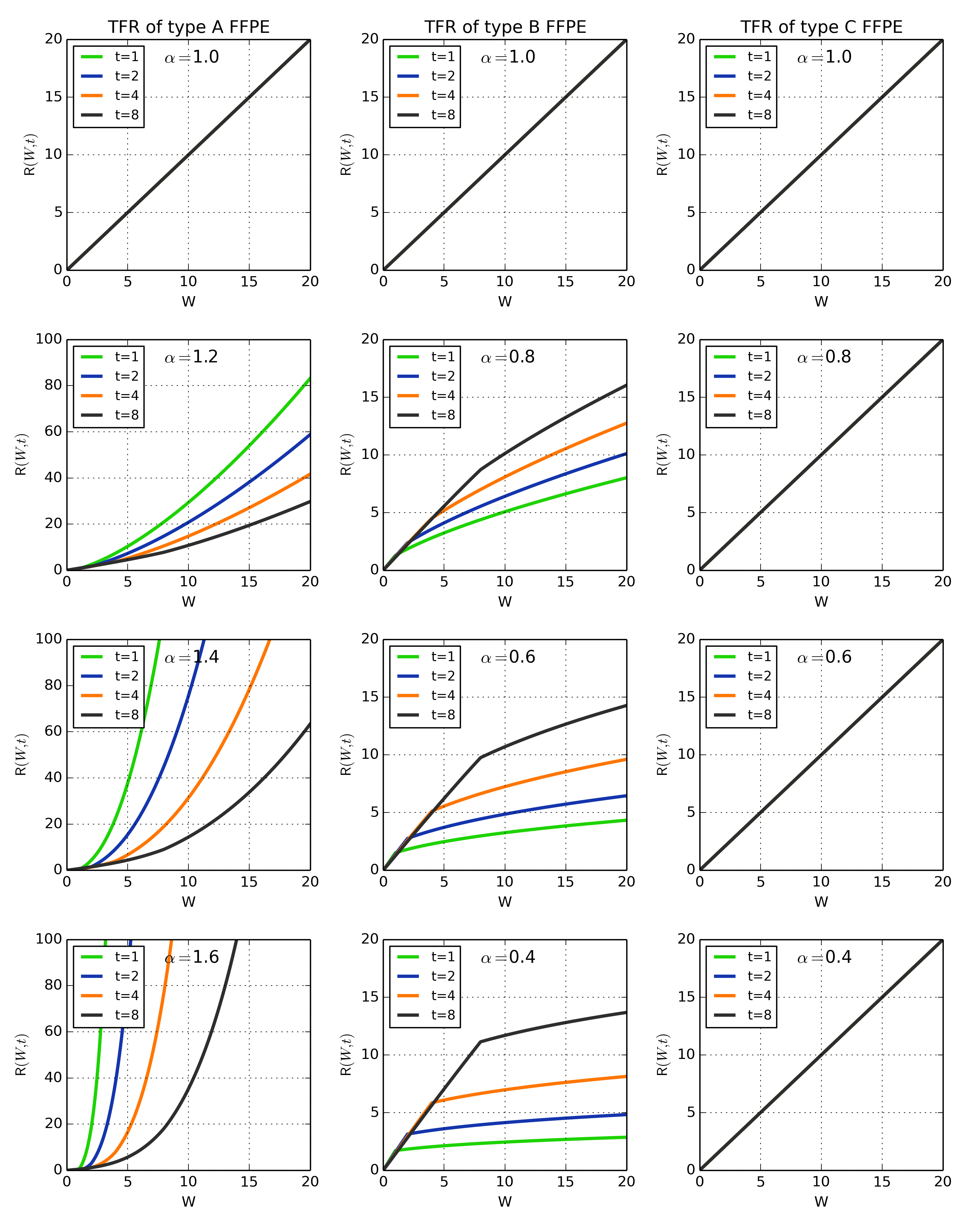
Figure 2: Time dependence of the fluctuation ratio for type A FFPE (left column), type B FFPE (middle column) and type C FFPE (right column) for different values of $\alpha$ (rows) and times $t=1,2,4,8$. Parameters were selected as $K_{\alpha}=1$, $v_{0}=1$ and $A_{\alpha}v_{0}=1$. Whereas $\alpha=1$ and all cases of $\alpha$ for type C FFPE show a normal fluctuation ratio with time-independent slope (in all of these cases the linear $t=8$ curve hides the previous times $t=1,2,4$) all other sub-plots show a more complex time- and work-dependent fluctuation ratio: Anomalous non-Markovian dynamics and/or non-Gaussian behavior cause a complicated time-dependence and non-linear behavior of the work fluctuation ratio.

3.3 Asymptotic expansions of the fluctuation ratio for type A and B FFPE

In this subsection we analyze the asymptotic behavior of the work fluctuation ratio for type A and B FFPE. Differences between type A and type B simply correspond to the value of $\alpha$ which is $1<\alpha<2$ for the superdiffusive FFPE of type A and $0<\alpha<1$ for the subdiffusive type B FFPE. Type C is not considered anymore, as the analytical calculation of Eq. 31 and the numerical analysis in Fig. 2 have delivered a normal fluctuation relation with a time-independent linear increase in the work $W$.

Small $W$ expansion:

First, the behavior of the TFR for the work PDFs of the FFPEs is studied for small $W$ as a function of time. The logarithmic ratio of a continuously differentiable function $p(z)$ can be expanded as Taylor series for positive $z$ as

$$\log\frac{p(z)}{p(-z)}=\frac{2}{p(z=0)}\left.\frac{dp(z)}{dz}\right|_{z=0}z+\mathcal{O}(z^{2}).$$ (35)

Inserting the approximate work PDF $p(W,t)$ from Eq. 25 together with the transformation of Eq. 27 into Eq. 35 requires the calculation of the derivative of the Fox $H$-function. Using Eq. 50 with $r=1$, $h=1$, $c=-1/\sqrt{K_{\alpha}t^{\alpha}}/F_{0}$, and $d=v_{0}t/\sqrt{K_{\alpha}t^{\alpha}}$ allows us to calculate the linear term in the Taylor expansion of Eq. 35. With the assumption $W/F_{0}<v_{0}t$ and after some simplifications using the definition of the Fox $H$-function by the Mellin-Barnes integral in Eq. 47 one obtains the fluctuation ratio for small $W$ as a quotient of two Fox $H$-functions:

$$\left.\mathsf{R}(W,t)\right|_{W\rightarrow 0}=\left(\frac{2}{v_{0}t}\right)\;\frac{\displaystyle H^{10}_{11}\left[\frac{v_{0}t}{\sqrt{K_{\alpha}t^{\alpha}}}\left|\begin{matrix}\displaystyle(1-\alpha/2,\alpha/2)\\ (1,1)\end{matrix}\right.\right]}{\displaystyle H^{10}_{11}\left[\frac{v_{0}t}{\sqrt{K_{\alpha}t^{\alpha}}}\left|\begin{matrix}\displaystyle(1-\alpha/2,\alpha/2)\\ (0,1)\end{matrix}\right.\right]}\;\frac{W}{F_{0}}=\Lambda(t)\;W.$$ (36)

The prefactor $\Lambda(t)$ summarizes the time-dependence of the fluctuation ratio. Its numerical evaluation based on the Taylor series of Eq. 49 is shown in Fig. 3A. In the superdiffusive case $1<\alpha<2$ (type A FFPE) the prefactor $\Lambda(t)$ increases as a function of time, whereas in the subdiffusive case it decreases with time. The argument of the Fox $H$-functions $z=v_{0}t/\sqrt{K_{\alpha}t^{\alpha}}$ in Eq. 36 scales $\sim t^{1-\alpha/2}$ with $1-\alpha/2>0$ for $0<\alpha<2$. Thus the asymptotic expansion of these Fox $H$-functions can be used for $t\rightarrow\infty$. In the long time limit the scaling function $\Lambda(t)$ converges towards the following non-zero constant value:

$$\lim_{t\rightarrow\infty}\Lambda(t)=2\left(\frac{2}{\alpha}\right)^{\alpha/(\alpha-2)}\left(\frac{v_{0}}{K_{\alpha}^{1/\alpha}}\right)^{\alpha/(2-\alpha)}\;\frac{W}{F_{0}}\rightarrow\frac{v_{0}}{K_{1}F_{0}}W\;\;\;\text{for}\;\;\;\alpha=1.$$ (37)

The corresponding values are shown as squares in Fig. 3A indicating the predicted asymptotic behavior. Fig. 3B shows the spatial behavior of the work fluctuation ratio for two subdiffusive examples $\alpha=0.4$ and $0.8$ at different instants of time $t$ (compare to small $W$ values in the overview given in Fig. 2). The slope of the ratio decreases with increasing time and agrees well with the small $W$ expansion given in Eq. 36. The superdiffusive case in Fig. 3C shows a reverse behavior as the small $W$ ratio increases with time. As indicated in Fig. 3A it can also be negative as show in Fig. 3C for $\alpha=1.6$ and $t=1,2$. In the superdiffusive case, the small $W$ expansion has a smaller region of agreement with the exact ratio. The more complex behavior is technically due to the two separating peaks of the PDF as illustrated in Fig. 1.

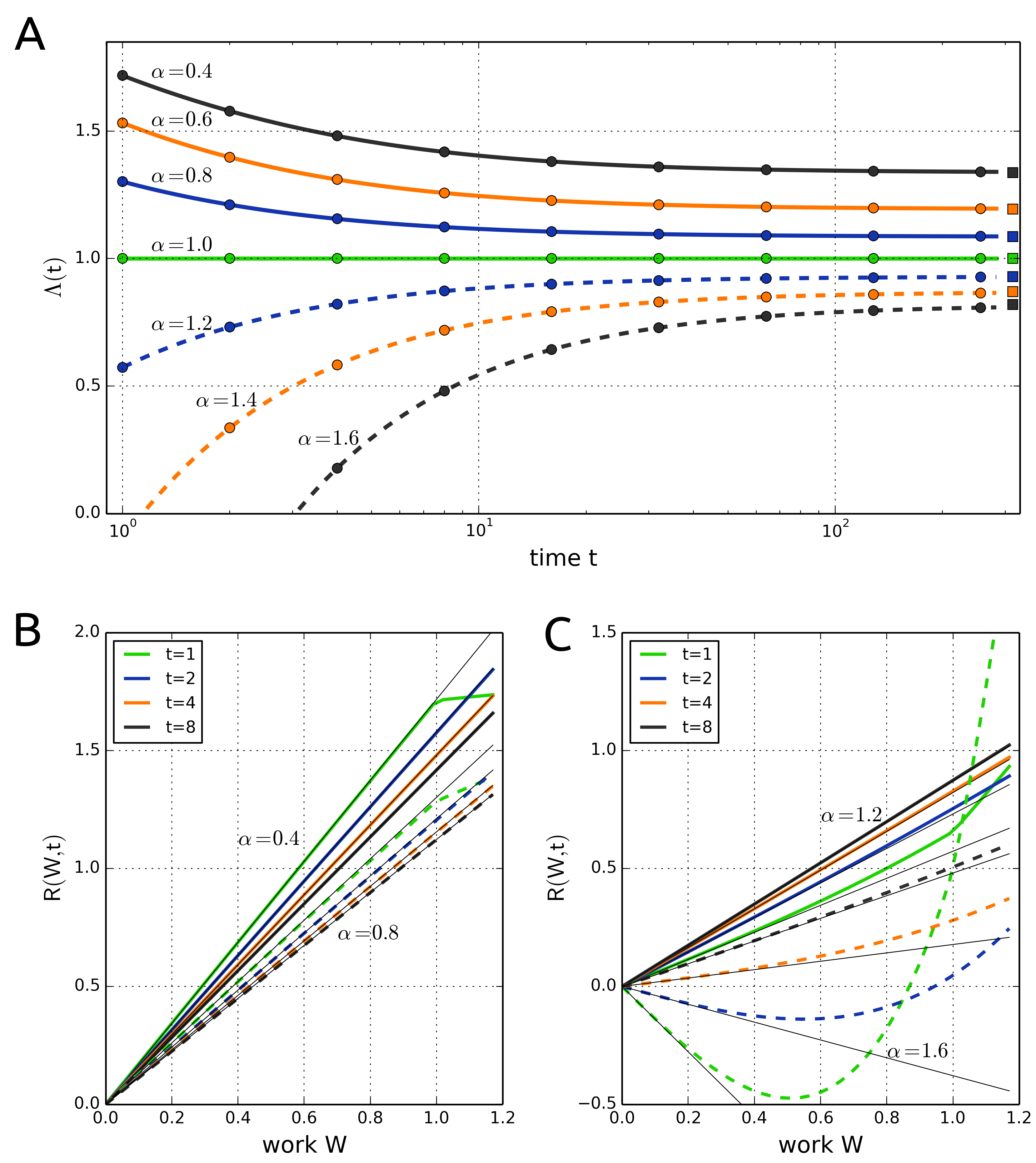
Figure 3: A. Time dependent decay of the initial fluctuation ratio $\Lambda(t)$ defined by Eq. 36 for small work $W$ and different values of $\alpha$ corresponding to type A FFPE ($1<\alpha<2$) and type B FFPE ($0<\alpha<1$) with parameters $K_{\alpha}=1$, $F_{0}=1$, $v_{0}=1$ and $A_{\alpha}v_{0}=1$. Circles show the direct calculation for small $W$ from the ratio of PDFs as defined in Eq. 28 whereas lines result from the computation of the first term of the small $W$ expansion of Eq. 35 and Eq. 36. Both calculations agree and $\Lambda(t)$ converges towards the long time limit given by Eq. 37 as indicated by the squares. Whereas $\Lambda(t)$ is time-independent for $\alpha=1$, it decrease or increases as a function of time for the subdiffusive (type B FFPE) and superdiffusive case (type A FFPE), respectively. B. The fluctuation ratio of work is shown for the subdiffusive case as a function of work and different time points as indicated. The slope decreases for increasing time. Thin black lines indicate the small work limit of Eq. 36. The obvious kink at $W=1$ for $t=1$ is due to the peak of the corresponding PDF in Fig. 1. C. The superdiffusive case shows a more complicated behavior: The small work slope increases with time. In addition, it also changes from negative to positive for small time in the $\alpha=1.6$ case.

Large $W$ expansion:

Finally, the behavior of the work fluctuation ratio is studied for large values of the work $W$. The overview given in Fig. 2 shows a different non-linear behavior for the subdiffusive and superdiffusive case. Assuming $W/F_{0}>v_{0}t$ and large arguments of the Fox $H$-function for type A and type B FFPE in Eq. 25 allows us to use the asymptotic expansion of the corresponding Fox $H$-function in Eq. 51. For large $W$ one obtains the following relation:

$$\left.\mathsf{R}(W,t)\right|_{W\rightarrow\infty}=\frac{2v_{0}t}{F_{0}}\;\left(\frac{\alpha}{2}\right)^{\alpha/(2-\alpha)}\left(\frac{1}{\sqrt{K_{\alpha}t^{\alpha}}}\right)^{2/(2-\alpha)}\;W^{\alpha/(2-\alpha)}.$$ (38)

Thus the work fluctuation ratio scales as a power law with an exponent $\alpha/(2-\alpha)$. This exponent is between $0$ and $1$ for the subdiffusive type B FFPE. For superdiffusive type A FFPE it is larger than $1$. This asymptotic power law behavior is shown in Fig. 4 for two examples. Continuous lines represent the result of Eq. 38 and agree for larger $W$ values with the exact results denoted by circles. Eq. 38 additionally contains a time-dependent scaling factor that is proportional $t^{(2\alpha-2)/(\alpha-2)}$. This factor is positive for the subdiffusive type B FFPE and negative for type A FFPE.

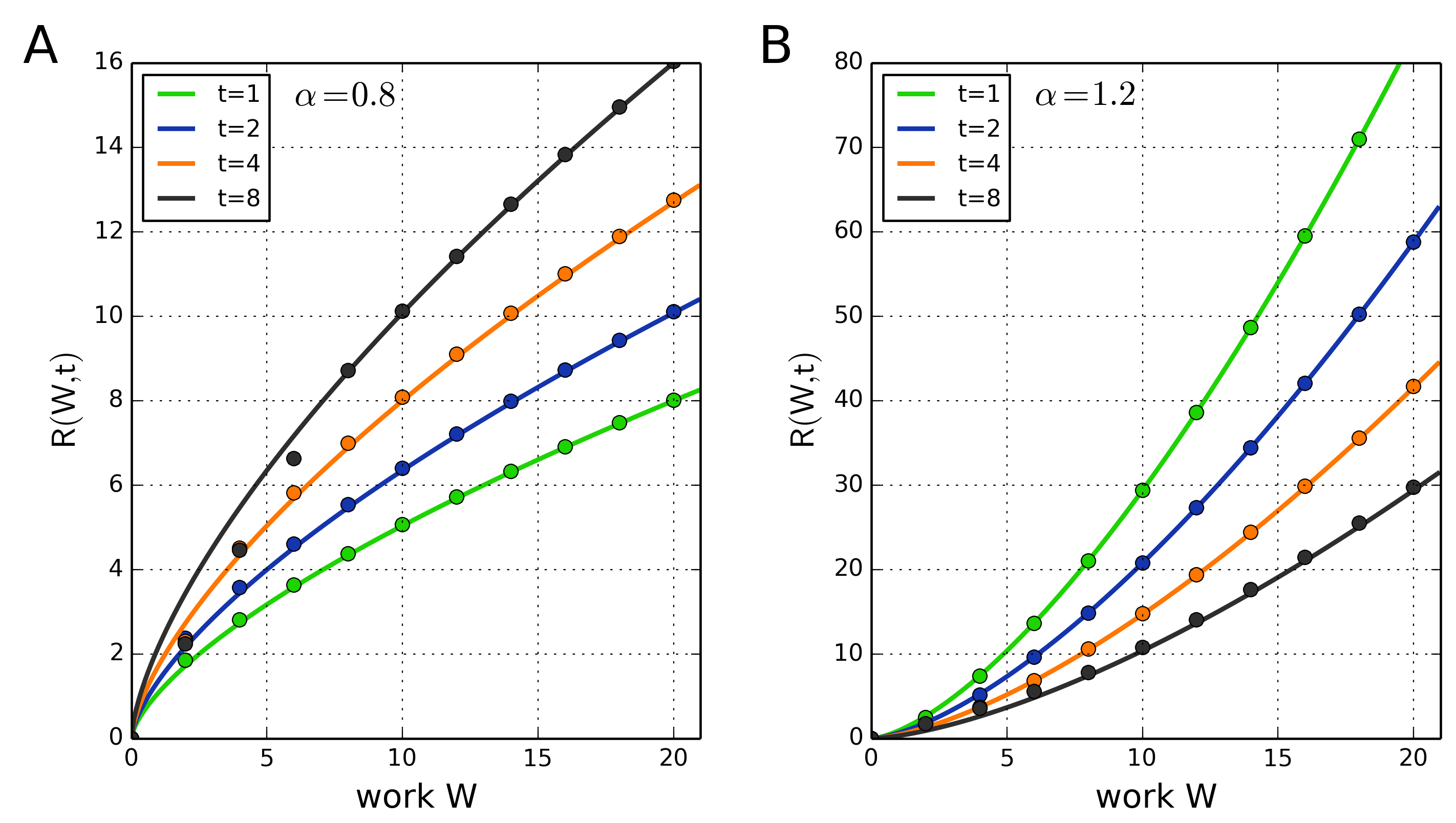
Figure 4: Large $W$ asymptotic of the work fluctuation ratio of type A and type B FFPEs. Continuous lines show the asymptotic large $W$ result given by Eq. 38. Circles indicate the exact result from the direct computation of the work fluctuation ratio. A. Subdiffusive case for $\alpha=0.8$ corresponding to type B FFPE. B. Superdiffusive case for $\alpha=1.2$ as example for type A FFPE.

4 Summary and outlook

In this work we studied three different types of FFPEs generating anomalous diffusion: a superdiffusive one (type A), a subdiffusive one (type B), and another one that exhibits a transition from sub- to superdiffusion under parameter variation (type C). Type A and type B break FDR1 while type C preserves it. Type A can be derived, under certain assumptions, from an overdamped Langevin equation with power law correlations of the velocity fluctuations, types B and C have been derived before in the literature from CTRW theory. Type C can also be obtained via subordination. We then calculated position PDFs for all models analytically and studied the shapes of all PDFs numerically under variation of the anomaly index as they evolve in time. Finally we checked the work TFR for all three models. Especially, we studied the time dependence of the ratio of the work fluctuations both for small and for large work by analytical asymptotic expansions in comparison to numerical evaluations.

We find that our type C model with FDR1 exhibits a conventional work TFR for all times, meaning the fluctuation ratio is constant in time and linear in the work. For a correlated Gaussian stochastic process it was shown that FDR1 implies the existence of a conventional TFR [43]. Our work generalises this result to an example of non-Gaussian PDFs generated by FFPE dynamics. It is interesting that the conventional TFR is still obeyed, despite the highly non-trivial dynamics exhibited by both the position PDFs and the corresponding moments. The existence of the conventional TFR for this case is connected to the fact that only the equation for Type C describes a subordinated process, namely the one subordinated to Brownian motion with drift under random time transformation. An important open question is to which extent Fig. 1 in [43] summarising the interplay between FDR1, FDR2 and TFRs for correlated Gaussian stochastic processes in terms of necessary and sufficient conditions can be generalised to non-Gaussian processes. For our other two models type A and type B the position PDFs show also very subtle and non-trivial non-Gaussian shapes. However, in contrast to type C they are characterised by a highly non-trivial fluctuation ratio: For type A the latter decreases with time, for type B it increases. Similar results have been obtained for the work TFR of strongly correlated Gaussian stochastic processes without FDR1 [42, 43]. On top of this, for both types of FFPEs the fluctuation ratio yields different long time limits depending on whether the work is small or large: For small work the fluctuation ratio converges to linearity in the work with constant prefactors, which reminds of the conventional TFR; however, here the slopes depend on the anomaly index of the dynamics. For large work the fluctuation ratio remains nonlinear in the work, with convex and concave shapes for type A and type B, respectively.

Our work was motivated by experiments on cell migration [50], where data were successfully fitted by solutions of a fractional Klein-Kramers equation [48]. Several generalisations of such a Klein-Kramers equation have been proposed to describe processes under external fields [48, 49, 51], which in turn yield FFPEs for the position only, similar to the ones studied in our paper, as special cases [21, 52, 12]. We thus believe that our present work might have important applications to understand cell migration in nonequilibrium situations such as under chemical gradients; see [44] for first results. More generally, our theory might have applications to understand glassy nonequilibrium dynamics: In computer simulations of a number of glassy systems violations of conventional TFRs have been observed featuring fluctuation ratios that are nonlinear in the work with time-dependent prefactors [40, 41].

Apart from such experimental applications, our first approach for deriving a FFPE pioneered by Balescu [57, 58] deserves to be studied in more detail. For example, it would be interesting to derive a superdiffusive FFPE from it that preserves FDR1, and to check again the TFR. On a broader scale it would be important to generalise our approach by considering more general observables, ideally dissipation functions [1] or related functionals defined within stochastic thermodynamics [7]. More general force fields than simply constant forces [42] and other types of FRs could be tested as well. Such theoretical studies may pave the way to identify different classes of anomalous FRs characterized by specific functional forms, generalized FDRs associated with them, and to explore the physical significance of these results. Last not least the quality of the Galilean invariant approximate solution Eq. 25 [20, 12] of the FFPEs 8,10 needs to be investigated in detail.

Appendix A Pseudo-Liouville approach

Following the so-called pseudo-Liouville hybrid approach of Balescu [57, 58] allows us to relate the dynamics of a particle defined by a Langevin equation to the corresponding PDF of the stochastic process. We start from the Langevin equation for the position $x(t)$ of a particle

$$\frac{dx(t)}{dt}=v_{0}+v(t)\>,$$ (39)

where $v(t)$ is a correlated stochastic process with zero mean $\langle v(t)\rangle=0$ and a given correlation function $\langle v(t)v(t^{\prime})\rangle=\mathsf{T}(t-t^{\prime})$, where the average is performed over the stochastic process $v(t)$. $v_{0}$ denotes a constant external force. The stochastic function $F(x,t)$

$$F(x,t)=\delta(x-x(t))$$ (40)

represents the exact density of the process. Derivation of Eq. 40 with respect to time and the usage of the Langevin equation Eq. 39 delivers the continuity equation for the exact density $F(x,t)$:

$$\frac{\partial F(x,t)}{\partial t}=-\frac{\partial}{\partial x}\delta(x-x(t))\;\frac{dx(t)}{dt}\longrightarrow\frac{\partial F(x,t)}{\partial t}+[v_{0}+v(t)]\frac{\partial F(x,t)}{\partial x}=0.$$ (41)

Now, the exact density $F(x,t)$ is decomposed into an averaged part $f(x,t)$ and fluctuations $\delta f(x,t)$

$$F(x,t)=f(x,t)+\delta f(x,t)\;\;\;\mbox{with}\;\;\;f(x,t)=\langle F(x,t)\rangle.$$ (42)

It is the further aim of this appendix to calculate the PDF $f(x,t)$ for the stochastic process defined by the Langevin equation Eq. 39 for given correlations of $v(t)$. Averaging of the exact density in Eq. 41 leads to

$$\left(\frac{\partial}{\partial t}+v_{0}\frac{\partial}{\partial x}\right)f(x,t)=-\frac{\partial}{\partial x}\big{\langle}v(t)\delta f(x,t)\big{\rangle}.$$ (43)

Subtraction of Eq. 43 from Eq. 41 results in

$$\left(\frac{\partial}{\partial t}+[v_{0}+v(t)]\frac{\partial}{\partial x}\right)\delta f(x,t)=-\frac{\partial}{\partial x}\bigg{(}v(t)\;f(x,t)-\big{\langle}v(t)\;\delta f(x,t)\big{\rangle}\bigg{)}.$$ (44)

Eq. 44 can be solved with the method of characteristics

$$\delta f(x,t)=-\frac{\partial}{\partial x}\int\limits_{0}^{t}dt^{\prime}\bigg{(}v(t^{\prime})\;f(x-\Delta(t,t^{\prime}),t^{\prime})-\big{\langle}v(t^{\prime})\;\delta f(x-\Delta(t,t^{\prime}),t^{\prime})\big{\rangle}\bigg{)}$$ (45)

with the definition $\Delta(t,t^{\prime})=v_{0}(t-t^{\prime})-\int\limits_{t^{\prime}}^{t}dt_{1}\;v(t_{1})$. Inserting Eq. 45 into Eq. 43 delivers the final equation for the PDF $f(x,t)$:

$$\left(\frac{\partial}{\partial t}+v_{0}\frac{\partial}{\partial x}\right)f(x,t)=\frac{\partial^{2}}{\partial x^{2}}\int\limits_{0}^{t}dt^{\prime}\big{\langle}v(t)v(t^{\prime})\;f(x-\Delta(t,t^{\prime}),t^{\prime})\big{\rangle}.$$ (46)

This is an exact relation for $f(x,t)$ that is generally non-local in space and non-local in time, i.e. non-Markovian. Applications and approximations of this relation are studied in section 2.1.

Appendix B Definiton and properties of Fox $H$-functions

The Fox $H$-function is defined as inverse Mellin transform of the function $\chi(s)$ [12, 71]

$$H_{p,q}^{m,n}(z)=H_{p,q}^{m,n}\left[z\bigg{|}\bigg{.}\begin{matrix}(a_{j},A_{j})_{j=1,p}\\ (b_{j},B_{j})_{j=1,q}\end{matrix}\right]=\frac{1}{2\pi i}\int_{\cal L}\chi(s)z^{s}ds$$ (47)

over a suitable path $\cal L$, with

$$\chi(s)=\frac{\prod\limits_{j=1}^{m}\Gamma(b_{j}-B_{j}s)\;\prod\limits_{j=1}^{n}\Gamma(1-a_{j}+A_{j}s)}{\prod\limits_{j=m+1}^{q}\Gamma(1-b_{j}+B_{j}s)\;\prod\limits_{j=n+1}^{p}\Gamma(a_{j}-A_{j}s)},$$ (48)

$0\leq n\leq p$, $1\leq m\leq q$, $(a_{j},b_{j})\in\mathbb{C}.$, and $(A_{j},B_{j})\in\mathbb{R}^{+}$. Empty products in Eq. 48 are taken as one.

A series expansion allows the numerical calculation of Fox $H$-functions. The following form for a special Fox $H$-function is used:

$$H^{10}_{11}\left[z\left|\begin{matrix}\displaystyle(a_{1},A_{1})\\ (b_{1},B_{1})\end{matrix}\right.\right]=\sum\limits_{k=0}^{\infty}\;\frac{(-1)^{k}}{\Gamma\left(\displaystyle a_{1}-A_{1}\frac{b_{1}+k}{B_{1}}\right)}\;\frac{\displaystyle z^{\frac{b_{1}+k}{B_{1}}}}{k!\;B_{1}}.$$ (49)

Summation in this work is performed numerically with multiple-precision arithmetic.

The derivation of the Fox $H$-function is required to calculate the fluctuation ratio for the FFPEs of type A and B. This can be performed using the following relation [72]:

$$\frac{d^{r}}{dx^{r}}H^{m,n}_{p,q} \left[(cx+d)^{h}\left|\begin{matrix}\displaystyle(a_{j},A_{j})_{1,p}\\ (b_{j},B_{j})_{1,q}\end{matrix}\right.\right]=$$ (50)

$$=\left(\frac{c}{cx+d}\right)^{r}\;H^{m,n+1}_{p+1,q+1}\left[(cx+d)^{h}\left|\begin{matrix}\displaystyle(0,h),(a_{j},A_{j})_{1,p}\\ (b_{j},B_{j})_{1,q},(r,h)\end{matrix}\right.\right].$$

For large arguments the Fox $H$-functions of type $H^{q,0}_{p,q}(z)$ decay as stretched exponential functions. The asymptotics of the PDF in Eq. 25 is given for large $z$ by [73, 72]

$$f_{A,B}(z,t)\sim\frac{z^{-\frac{1-\alpha}{2-\alpha}}}{\sqrt{4\pi(2-\alpha)K_{\alpha}t^{\alpha}}}\left(\frac{2}{\alpha}\right)^{\frac{1-\alpha}{2-\alpha}}\;\exp\bigg{\{}-\left(\frac{2-\alpha}{2}\right)\;\left(\frac{2}{\alpha}\right)^{\frac{\alpha}{\alpha-2}}\;z^{\frac{2}{2-\alpha}}\bigg{\}}$$ (51)

for $z\rightarrow\infty$ and $z=|x-v_{0}t|/\sqrt{K_{\alpha}t^{\alpha}}$.

References

References

- [1] D.J. Evans and D.J. Searles. The fluctuation theorem. Adv. Phys., 51:1529–1585, 2002.
- [2] C. Bustamante, J. Liphardt, and F. Ritort. The nonequilibrium thermodynamics of small systems. Phys. Today, 58:43–48, 2005.
- [3] R.J. Harris and G.M. Schütz. Fluctuation theorems for stochastic dynamics. J. Stat. Mech. Theor. Exp., 7:P07020/1–45, 2007.
- [4] M. Esposito, U. Harbola, and S. Mukamel. Nonequilibrium fluctuations, fluctuation theorems, and counting statistics in quantum systems. Rev. Mod. Phys., 81:1665–1702, 2009.
- [5] M. Campisi, P. Hänggi, and P. Talkner. Quantum fluctuation relations: Foundations and applications. Rev. Mod. Phys., 83:771–791, 2011.
- [6] V Jaksic, C-A Pillet, and L Rey-Bellet. Entropic fluctuations in statistical mechanics: I. Classical dynamical systems. Nonlinearity, 24:699–763, 2011.
- [7] U. Seifert. Stochastic thermodynamics, fluctuation theorems and molecular machines. Rep. Progr. Phys., 75(12):126001/1–58, 2012.
- [8] R. Klages, W. Just, and C. Jarzynski, editors. Nonequilibrium statistical physics of small systems: Fluctuation relations and beyond. Wiley-VCH, Berlin, 2013.
- [9] C. Maes. On the origin and the use of fluctuation relations for the entropy. Séminaire Poincaré, 2:29–62, 2003.
- [10] K. Sekimoto. Stochastic Energetics. Lecture Notes in Physics. Springer, Berlin, 2010.
- [11] C. van den Broeck. Stochastic thermodynamics: A brief introduction. In F. Sciortino C. Bechinger and P. Ziherl, editors, Physics of Complex Colloids, volume 184 of Proceedings of the International School of Physics ”Enrico Fermi”, pages 155–193, Amsterdam, 2013. IOS Press.
- [12] R. Metzler and J. Klafter. The random walk’s guide to anomalous diffusion: A fractional dynamics approach. Phys. Rep., 339:1–77, 2000.
- [13] W. Coffey, Y.P. Kalmykov, and J.T. Waldron. The Langevin Equation. World Scientific, Singapore, 2004.
- [14] R. Metzler and J. Klafter. The restaurant at the end of the random walk: Recent developments in the description of anomalous transport by fractional dynamics. J. Phys. A: Math. Gen., 37:R161–R208, 2004.
- [15] R. Klages, G. Radons, and I.M. Sokolov, editors. Anomalous Transport: Foundations and Applications. Wiley-VCH, Berlin, 2008.
- [16] J. Klafter and I.M. Sokolov. First Steps in Random Walks: From Tools to Applications. Oxford University Press, Oxford, 2011.
- [17] V. Zaburdaev, S. Denisov, and J. Klafter. Lévy walks. preprint arXiv:1410.5100, 2015.
- [18] A. Compte. Continuous time random walks on moving fluids. Phys. Rev. E, 55:6821–6831, 1997.
- [19] A. Compte, R. Metzler, and J. Camacho. Biased continuous time random walks between parallel plates. Phys. Rev. E, 56:1445–1454, 1997.
- [20] R. Metzler, J. Klafter, and I.M. Sokolov. Anomalous transport in external fields: Continuous time random walks and fractional diffusion equations extended. Phys. Rev. E, 58:1621–1633, 1998.
- [21] E. Lutz. Fractional Langevin equation. Phys. Rev. E, 64:051106/1–4, 2001.
- [22] I. Goychuk. Viscoelastic subdiffusion: Generalized Langevin equation approach. Adv. Chem. Phys., 150:187–253, 2012.
- [23] J.-H. Jeon, A.V. Chechkin, and R. Metzler. First passage behaviour of multi-dimensional fractional Brownian motion and application to reaction phenomena. In G. Oshanin, S. Redner, and R. Metzler, editors, First passage problems: recent advances, pages 175–202, Singapore, 2014. World Scientific.
- [24] J. Klafter, A. Blumen, and M. F. Shlesinger. Stochastic pathway to anomalous diffusion. Phys. Rev. A, 35:3081–3085, 1987.
- [25] S. C. Lim and S. V. Muniandy. Self-similar Gaussian processes for modeling anomalous diffusion. Phys. Rev. E, 66:021114/1–14, 2002.
- [26] J.-H. Jeon, A.V. Chechkin, and R. Metzler. Scaled Brownian motion: a paradoxical process with a time dependent diffusivity for the description of anomalous diffusion. Phys. Chem. Chem. Phys., 16:15811–15817, 2014.
- [27] A.G. Cherstvy, A.V. Chechkin, and R. Metzler. Particle invasion, survival, and non-ergodicity in 2D diffusion processes with space-dependent diffusivity. Soft Matter, 10:1591–1601, 2014.
- [28] F. Zamponi, F. Bonetto, L.F. Cugliandolo, and J. Kurchan. A fluctuation theorem for non-equilibrium relaxational systems driven by external forces. J. Stat. Mech. Theor. Exp., 09:P09013/1–51, 2005.
- [29] T. Ohkuma and T. Ohta. Fluctuation theorems for non-linear generalized Langevin systems. J. Stat. Mech. Theor. Exp., 10:P10010/1–28, 2007.
- [30] T. Mai and A. Dhar. Nonequilibrium work fluctuations for oscillators in non-Markovian baths. Phys. Rev. E, 75:061101/1–7, 2007.
- [31] S. Chaudhury, D. Chatterjee, and B.J. Cherayil. Resolving a puzzle concerning fluctuation theorems for forced harmonic oscillators in non-Markovian heat baths. J. Stat. Mech. Theor. Exp., 2008(10):P10006/1–13, 2008.
- [32] T. Speck and U. Seifert. The Jarzynski relation, fluctuation theorems, and stochastic thermodynamics for non-Markovian processes. J. Stat. Mech. Theor. Exp., 2007:L09002/1–10, 2007.
- [33] C. Beck and E.G.D. Cohen. Superstatistical generalization of the work fluctuation theorem. Physica A, 344:393–402, 2004.
- [34] A. Baule and E.G.D. Cohen. Fluctuation properties of an effective nonlinear system subject to Poisson noise. Phys. Rev. E, 79:030103/1–4, 2009.
- [35] H. Touchette and E.G.D. Cohen. Fluctuation relation for a Lévy particle. Phys. Rev. E, 76:020101(R)/1–4, 2007.
- [36] H. Touchette and E.G.D. Cohen. Anomalous fluctuation properties. Phys. Rev. E, 80:011114/1–11, 2009.
- [37] A.A. Budini. Generalized fluctuation relation for power-law distributions. Phys. Rev. E, 86:011109/1–12, 2012.
- [38] L. Kusmierz, J.M. Rubi, and E. Gudowska-Nowak. Heat and work distributions for mixed Gauss-Cauchy process. J. Stat. Mech. Theor. Exp., 2014(9):P09002/1–25, 2014.
- [39] M. Esposito and K. Lindenberg. Continuous-time random walk for open systems: Fluctuation theorems and counting statistics. Phys. Rev. E, 77:051119/1–12, 2008.
- [40] M. Sellitto. Fluctuation relation and heterogeneous superdiffusion in glassy transport. Phys. Rev. E, 80:011134/1–5, 2009.
- [41] A. Crisanti, M. Picco, and F. Ritort. Fluctuation relation for weakly ergodic aging systems. Phys. Rev. Lett., 110:080601/1–5, 2013.
- [42] A.V. Chechkin and R. Klages. Fluctuation relations for anomalous dynamics. J. Stat. Mech. Theor. Exp., 2009(03):L03002/1–11, 2009.
- [43] A.V. Chechkin, F. Lenz, and R. Klages. Normal and anomalous fluctuation relations for Gaussian stochastic dynamics. J. Stat. Mech. Theor. Exp., 2012(11):L11001/1–13, 2012.
- [44] R. Klages, A.V. Chechkin, and P. Dieterich. Anomalous fluctuation relations. In R. Klages, W. Just, and C. Jarzynski, editors, Nonequilibrium statistical physics of small systems: Fluctuation relations and beyond, pages 259–282, Berlin, 2013. Wiley-VCH.
- [45] R. Kubo, M. Toda, and N. Hashitsume. Statistical Physics, volume 2 of Solid State Sciences. Springer, Berlin, 2nd edition, 1992.
- [46] I.M. Sokolov, J. Klafter, and A. Blumen. Fractional kinetics. Phys. Today, 55:48–54, 2002.
- [47] H.C. Fogedby. Langevin equations for continuous time Lévy flights. Phys. Rev. E, 50:1657–1660, 1994.
- [48] E. Barkai and R. Silbey. Fractional Kramers equation. J. Phys. Chem. B, 104:3866 –3874, 2000.
- [49] R. Metzler and I.M. Sokolov. Superdiffusive Klein-Kramers equation: Normal and anomalous time evolution and Lévy walk moments. Europhys. Lett., 58:482–488, 2002.
- [50] P. Dieterich, R. Klages, R. Preuss, and A. Schwab. Anomalous dynamics of cell migration. PNAS, 105:459–463, 2008.
- [51] R. Friedrich, F. Jenko, A. Baule, and S. Eule. Anomalous diffusion of inertial, weakly damped particles. Phys. Rev. Lett., 96:230601/1–4, 2006.
- [52] W.R. Schneider and W.Wyss. Fractional diffusion and wave equations. J. Math. Phys, 30:134 –144, 1989.
- [53] E. Barkai, Y. Garini, and R. Metzler. Strange kinetics of single molecules in living cells. Phys. Today, 65:29–35, 2012.
- [54] N. Korabel, A.V. Chechkin, R. Klages, I.M. Sokolov, and V.Yu. Gonchar. Understanding anomalous transport in intermittent maps: From continuous time random walks to fractals. Europhys. Lett., 70:63–69, 2005.
- [55] N. Korabel, R. Klages, A.V. Chechkin, I.M. Sokolov, and V.Yu. Gonchar. Fractal properties of anomalous diffusion in intermittent maps. Phys. Rev. E, 75:036213/1–14, 2007.
- [56] D. Brockmann1, L. Hufnagel, and T. Geisel. The scaling laws of human travel. Nature, 439:462–465, 2006.
- [57] R. Balescu. Statistical dynamics: matter out of equilibrium. Imperial College Press, 1997.
- [58] R. Balescu. V-Langevin equations, continuous time random walks and fractional diffusion. Chaos, Solitons & Fractals, 34:62 – 80, 2007.
- [59] O.I. Marichev S.G. Samko, A.A. Kilbas. Fractional Integrals and Derivatives: Theory and Applications. Gordon and Breach, Amsterdam, 1993.
- [60] B.J. West, P. Grigolini, R. Metzler, and T.F. Nonnenmacher. Fractional diffusion and Lévy stable processes. Phys. Rev. E, 55:99–106, 1997.
- [61] R. Metzler and J. Klafter. From a generalized Chapman−Kolmogorov equation to the fractional Klein−Kramers equation†. J. Phys. Chem. B, 104:3851–3857, 2000.
- [62] R. Metzler and J. Klafter. Accelerating Brownian motion: A fractional dynamics approach to fast diffusion. Europhys. Lett., 51:492–498, 2000.
- [63] R. Gorenflo, Y. Luchko, and F. Mainardi. Wright functions as scale-invariant solutions of the diffusion-wave equation. J. Comput. Appl. Math., 118:175–191, 2000.
- [64] G.Guo, A. Bittig, and A. Uhrmacher. Lattice monte carlo simulation of galilei variant anomalous diffusion. J. Comput. Phys., 288:167––180, 2015.
- [65] R. Metzler and A. Compte. Generalized diffusion-advection schemes and dispersive sedimentation: a fractional approach. J. Phys. Chem. B, 104:3858–3865, 2000.
- [66] A. Cairoli and A. Baule. To be published. 2015.
- [67] E. Barkai. Fractional Fokker-Planck equation, solution, and application. Phys. Rev. E, 63:046118/1–17, 2001.
- [68] A. Talbot. The accurate numerical inversion of Laplace transforms. IMA J Appl Math, 23(1):97–120, January 1979.
- [69] J. Abate and P. P. Valkó. Multi-precision Laplace transform inversion. International Journal for Numerical Methods in Engineering, 60:979–993, 2004.
- [70] A. Baule and R. Friedrich. Joint probability distributions for a class of non-markovian processes. Phys. Rev. E, 71:026101/1–9, 2005.
- [71] F. Mainardi, G. Pagnini, and R. K. Saxena. Fox H functions in fractional diffusion. J. Comput. Appl. Math., 178:321–331, 2005.
- [72] A. M. Mathai, R. K. Saxena, and Haubold H. J. The H-Function: Theory and Applications. Springer New York, 2010.
- [73] B. L. J. Braaksma. Asymptotic expansions and analytic continuations for a class of Barnes-integrals. Compositio Mathematica, 15:239–341, 1962-1964.