MMSE of probabilistic low-rank matrix estimation:
Universality with respect to the output channel.

Abstract

This paper considers probabilistic estimation of a low-rank matrix from non-linear element-wise measurements of its elements. We derive the corresponding approximate message passing (AMP) algorithm and its state evolution. Relying on non-rigorous but standard assumptions motivated by statistical physics, we characterize the minimum mean squared error (MMSE) achievable information theoretically and with the AMP algorithm. Unlike in related problems of linear estimation, in the present setting the MMSE depends on the output channel only trough a single parameter – its Fisher information. We illustrate this striking finding by analysis of submatrix localization, and of detection of communities hidden in a dense stochastic block model. For this example we locate the computational and statistical boundaries that are not equal for rank larger than four.

I Introduction

Estimation of low-rank matrices from their noisy or incomplete measurements is a problem that has a wide range of applications of practical interest [1]. As for every broadly relevant data processing problem it is of interest to study statistical and computational limits of such an estimation on meaningful model settings. In this paper we evaluate the Bayes optimal and computationally achievable mean-squared error of estimation for the following two models:

In the first model the matrix to be estimated is created as

$$W=\frac{1}{\sqrt{n}}XKX^{T}\,,$$ (1)

where $X$ is a $n\times r$ matrix whose rows $x_{i}$ were chosen independently at random from some distribution $P_{\rm prior}(x_{i})$, and $K$ is a $r\times r$ symmetric matrix. The matrix $W$ is then observed element-wise trough a noisy non-linear output channel $P_{\rm out}(y_{ij}|w_{ij})$, with $i,j=1,\dots,n$. The goal is to estimate the unknown matrix $X$ from measured $Y$.

We consider the problem in the limit of very large systems $n\to\infty$, small rank $r=\Omega(1)$, and $\partial P_{\rm out}/\partial w=\Omega(1)$. The purpose of the scaling factor $1/\sqrt{n}$ in (1) is that the inference problem is neither trivially easy nor clearly impossible in this limit. The same model and scaling was considered e.g. in [2, 3], where the matrix $K$ was an identity. The main algorithmic difficulty in such a setting comes from the high dimension $n$. In this work we study the idealized setting in which the hyper-parameters $r,K,P_{\rm prior},P_{\rm out}$ are independent of the dimension $n$ and known. Note, however, that extending our approach via expectation maximization seems like a natural way to learn these hyper-parameters.

In the second model the matrix to be estimated is created as

$$W=\frac{1}{\sqrt{n}}UV^{T}\,,$$ (2)

where $U$ is a $n\times r$ matrix and $V$ is a $m\times r$ matrix, with rows $u_{i}$ (resp. $v_{i}$) chosen from some distribution $P^{u}_{\rm prior}(u_{i})$ (resp. $P^{v}_{\rm prior}(v_{i})$). The matrix $W$ is then observed trough the same output channel $P_{\rm out}(y_{ij}|w_{ij})$ as above, and the problem is set analogously, adding that $m/n=\alpha=\Omega(1)$. Most of the discussion in this paper uses notation of the first model, but all our results are relevant for the second one as well.

An algorithmic tool that first comes to our mind when seeing the setting above is singular (or eigenvalue) value decomposition (SVD) keeping the leading $r$ components. SVD is the optimal estimation algorithm if the goal is to minimize the mean squared distance between the observed matrix $Y$ and the estimator irrespectively of the properties of the factors (such as the prior $P_{\rm prior}$). Requirements on the factors, such as sparsity or other structure are not incorporated in the basic SVD. Moreover, for a general non-linear output channel $P_{\rm out}$ the sum of squares between $Y$ and its estimator is not the most relevant quantity to minimize.

Setting the problem in a fully probabilistic way is another common approach [4], that is in principle much more flexible, but algorithmically more challenging in general. To obtain a Bayes-optimal estimator of the factor $x_{i}$ ($r$-dimensional column vector) we need to compute the marginals of the posterior probability distribution

$$P(X|Y)=\frac{1}{Z(Y)}\prod_{1\leq i\leq n}P_{\rm prior}(x_{i})\prod_{1\leq i\leq j\leq n}P_{\rm out}(y_{ij}|w_{ij})\,,$$ (3)

where $w_{ij}=x^{T}_{i}Kx_{j}/\sqrt{n}$. In this paper we will leverage this algorithmic difficulty by realizing that techniques based on approximate message passing and related state evolution (SE) are asymptotically optimal for the above setting. For compressed sensing these techniques are rigorous thanks to series of works [5, 6]. The AMP algorithm and its state evolution for the above setting is different from the one of compressed sensing, and these proofs do not apply. Arguments for the optimality in the present setting come from non-rigorous methods of statistical physics. From a mathematical point of view the present paper provides a set of accurate conjectures. Fully rigorous proof of these conjectures is a natural direction for future work.

I-A Examples

The above model includes a number of examples that are commonly considered in the literature. Without trying to be exhaustive, we list a few interesting ones.

• Sparse principle component analysis as considered in [2, 3]: The prior distribution $P_{\rm prior}$ has a weight $1-\rho$ on a vector of zeros. The output channel was considered as additive Gaussian noise.

• Robust PCA [7] in which the measured matrix is a low-rank matrix plus a sparse large noise: The output channel adds small noise with some probability $p$ and large noise with $1-p$.

• Submatrix localization [8, 9]: The matrix $W$ includes $r$ submatrices (overlapping or not) that have larger mean than the overall mean of the matrix $W$. The prior $x_{i}$ then encodes in a binary manner to which of the $r$ submatrices does a given variable $i$ belong. The output is usually considered as Gaussian additive noise.

• Detection of communities hidden in dense networks: Stochastic block model is popular for theoretical studies of clustering. Nodes belong to different clusters/communities, the prior $P_{\rm prior}$ then allows only vectors having one component $1$, and $0$ elsewhere. The observed matrix $Y$ is binary and the probability to observe $y_{ij}=1$ is given by $K_{ab}$ if $x_{i}(a)=1$ and $x_{j}(b)=1$ ($i,j=1,\dots,n$, and $a,b=1,\dots,r$).

• Biclustering is a simultaneous clustering of rows and columns, it finds a number of applications e.g. for analysis of microarray data in genomics [10]. Again the prior encodes affinity to a cluster and the output function includes various models of noise.

• Poisson noise in the matrix factorization was considered e.g. in [11].

• The labeled stochastic block model is another case that can be reformulated in the present setting [12].

I-B Contribution and closely related work

As far as we know the only tools that provides asymptotically exact analysis of the minimal mean squared error of models (1-2) is approximate message passing and state evolution as deployed in the present paper. For the output channel being additive Gaussian noise this was done previously in [13, 2] for rank $r=1$ with part of the results being fully rigorous, in [14] for generic rank and without the state evolution, and in [3] for general rank with the state evolution, but non-rigorously. The main contribution of this paper is the treatment of the case of general non-linear output channel $P_{\rm out}$.

Approximate message passing and state evolution for a generic output channel $P_{\rm out}$ was derived previously in the context of linear estimation [15], and later in matrix factorization with $r=\Omega(n)$ [16]. In both these cases the resulting equations (both the AMP and the state evolution) are considerably more involved than those for additive Gaussian noise. In the setting of low-rank models (1-2) above the situation is remarkably simpler as the AMP algorithm stays the same up to a change of the matrix $Y$ for the so-called Fisher score matrix $S$ that depends on the output channel and on $Y$ element-wise, and the inverse of the Fisher information of the channel that we denote $\Delta$ and plays a role of an effective noise variance. In the state evolution the situation is even simpler in the sense that only the effective value $\Delta$ of the noise appears.

The space of all the possible element-wise output channels hence reduces to one dimensional space, parametrized by their inverse Fisher information $\Delta$. The resulting asymptotic MMSE depends only on $\Delta$ and not on other details of the channel. Consequently, classes of rather differently looking matrix estimation problems all share the same single-letter characterization. The contribution of the present paper is to unveil and quantify this property, and illustrate it on the example of detection of communities hidden in dense networks that is via this one parameter mapping related to localization of submatrices having different mean from the background matrix.

Analogous universality with respect to the output channel was observed in [17] (see e.g. their remark 2.5) in the study of detection of a small hidden clique with approximate message passing.

Our results for the Bayes-optimal estimation error of community detection in dense stochastic block model are of independent interest. Analogous results were derived for the sparse case in [18]. In the dense case only MSE-suboptimal spectral methods were evaluated [19]. We also unveil a hard phase existing in this problem for rank $r>4$, and becoming very wide for $r\to\infty$.

We also recently learned about independently ongoing work of [20] who consider rank $r=1$ with Radamacher prior, and establish rigorously the relation between the stochastic block model with two groups and low-rank estimation with Gaussian channel.

II AMP and state evolution

II-A From belief propagation to AMP

In this section we derive the AMP algorithm to compute marginals of the posterior probability distribution (3). We present the derivation for the $XKX^{\top}$ case, for the $UV^{\top}$ everything works analogously and we only state the results. For convenience we introduce a function $g(y,w)$ as

$$P_{\rm out}(y|w)=e^{g(y,w)}\,.$$ (4)

We require $g(y,w)$ to be differentiable in $w$. For the previously considered Gaussian additive noise we have $g_{\rm GAN}(y,w)=-(y-w)^{2}/(2\Delta)$.

In the first step, we write the belief propagation equations for the probability distribution (3). For this we introduce messages ${m^{t}_{ij\rightarrow i}}(x_{i})$ and $n_{i\rightarrow ij}^{t}(x_{i})$ between variables $x_{i}$ and the factors associated to $y_{ij}$. The BP equations read

$${m^{t}_{il\rightarrow i}}(x_{i})=\frac{1}{Z^{t}_{il\to i}}\int{\rm d}x_{l}\,{n^{t}_{l\rightarrow il}}(x_{l})\,e^{g\left(y_{il},\frac{1}{\sqrt{n}}x_{l}^{\top}Kx_{i}\right)}\,,\\ {n^{t+1}_{i\rightarrow ij}}(x_{i})=\frac{1}{Z^{t}_{i\to ij}}P_{\rm prior}(x_{i})\prod\limits_{l\neq i,l\neq j}{m^{t}_{il\rightarrow i}}(x_{i})\,,$$ (5)

where $Z^{t}_{il\to i}$ and $Z^{t}_{i\to ij}$ are normalizations. The main assumption behind these BP equations is that the messages $n_{i\rightarrow il}(x_{i})$ and $n_{i\rightarrow ij}(x_{i})$ can be interpreted as probabilities that are statistically independent conditioned to the values of the variable $x_{i}$ in the large $n$ limit. This is also the main assumption of this paper. Arguments of theoretical statistical physics [21] provide heuristic justification for this assumption. In the above form the BP equations are not useful for implementation. We, however, realize that we can rewrite them into a much simpler form that provides the same marginals in the limit of large $n$.

In the large $n$ limit the function $g\left(y_{il},x_{l}^{\top}Kx_{i}/\sqrt{n}\right)$ depends only weakly on $x_{i}$ and $x_{l}$. Therefore we expand this function around $w=0$ and (5) then becomes

$$\frac{{m^{t}_{il\rightarrow i}}(x_{i})}{\exp(g(y_{il},0))}\propto 1+\frac{1}{\sqrt{n}}\frac{\partial g}{\partial w}\Big{|}_{y_{il},0}{a_{l\rightarrow il}^{t}}^{\top}Kx_{i}+\\ \frac{1}{2n}h(y_{il})x_{i}^{\top}K\left(v_{l\rightarrow il}^{t}+a_{l\rightarrow il}^{t}{a_{l\rightarrow il}^{t}}^{\top}\right)Kx_{i}+O\left({n^{-\frac{3}{2}}}\right)\,,$$ (6)

where

$$h(y_{il})=\frac{\partial^{2}g}{\partial w^{2}}\Big{|}_{y_{il},0}+\left(\frac{\partial g}{\partial w}\Big{|}_{y_{il},0}\right)^{2}\,.$$ (7)

Here we introduced quantities $a^{t}_{l\rightarrow il}$ and $v^{t}_{l\rightarrow il}$ as the mean and covariance of $n^{t}_{l\rightarrow il}$ We then take the logarithm of (6) and by using (5) we find

$${n^{t+1}_{i\rightarrow ij}}(x_{i})=P_{\rm prior}(x_{i})e^{{B^{t}_{i\rightarrow ij}}^{\top}x_{i}-\frac{x_{i}^{\top}A_{i\rightarrow ij}^{t}x_{i}}{2}}\,,$$ (8)

where

$$B^{t}_{i\rightarrow ij}=\frac{K}{\sqrt{n}}\sum\limits_{l\neq i,j}\frac{\partial g}{\partial w}\Big{|}_{y_{il},0}{a_{l\rightarrow il}^{t}}\,,$$ (9)

$$A^{t}_{i\rightarrow ij}=\frac{K}{n}\Big{\{}\sum\limits_{l\neq i,j}\left(\frac{\partial g}{\partial w}\Big{|}_{y_{il},0}\right)^{2}a_{l\rightarrow il}^{t}{{a_{l\rightarrow il}^{t}}^{\top}}+$$

$$\sum\limits_{l\neq i,j}h(y_{il})\left(v_{l\rightarrow il}^{t}+a_{l\rightarrow il}^{t}{a^{t}_{l\rightarrow il}}^{\top}\right)\Big{\}}K\,.$$ (10)

To close these equations we finally compute the new mean and variance of the messages $n_{i\rightarrow ij}^{t+1}$ as

$$a_{i\rightarrow ij}^{t+1}=f(A_{i\rightarrow ij}^{t},B_{i\rightarrow ij}^{t})\,,$$ (11)

$$v_{i\rightarrow ij}^{t+1}=\left(\frac{\partial f}{\partial B}\right)(A_{i\rightarrow ij}^{t},B_{i\rightarrow ij}^{t})\,,$$ (12)

where $f(A,B)$ is the mean of the normalized probability distribution

$$P(x)=\frac{1}{{\cal Z}(A,B)}P_{\rm prior}(x)\exp\left(B^{\top}x-\frac{x^{\top}Ax}{2}\right)$$ (13)

and $\partial f/\partial B$ is its covariance matrix. Above we closed the intractable distributional belief propagation equations on the means and variances of the messages.

As we can already anticipate it will be instrumental to introduce the so-called Fisher score matrix (evaluated at $w=0$) as

$$S_{ij}\equiv\frac{\partial\log P_{\rm out}(y_{ij}|w)}{\partial w}\Big{|}_{y_{ij},0}\,,$$ (14)

and the Fisher information (evaluated at $w=0$) of the output channel as

$$\frac{1}{\Delta}\equiv\mathbb{E}_{P_{\rm out}(y|w=0)}\left[\left(\frac{\partial\log P_{\rm out}(y|w)}{\partial w}\Big{|}_{y,0}\right)^{2}\right]\,.$$ (15)

We denote the inverse Fisher information by $\Delta$ because that would be the noise variance for the Gaussian additive channel (in that case $S=Y/\Delta$).

Using $\int{\rm d}yP_{\rm out}(y|w)=1$, $\forall w$ and (4), it follows that

$$\mathbb{E}_{P_{\rm out}(y|w=0)}\left(\frac{\partial g}{\partial w}\Big{|}_{y,0}\right)=0\,,$$ (16)

$$\mathbb{E}_{P_{\rm out}(y|w=0)}\left[\left(\frac{\partial g}{\partial w}\Big{|}_{y,0}\right)^{2}+\frac{\partial^{2}g}{\partial w^{2}}\Big{|}_{y,0}\right]=0\,.$$ (17)

With the above, eqs. (10) can be rewritten as

$$B^{t}_{i\rightarrow ij}=\frac{K}{\sqrt{n}}\sum\limits_{l\neq i,j}S_{il}{a_{l\rightarrow il}^{t}}\,,$$ (18)

$$A^{t}_{i\rightarrow ij}=\frac{K}{n\Delta}\left[\sum\limits_{l\neq i,j}a_{l\rightarrow il}^{t}{{a_{l\rightarrow il}^{t}}^{\top}}\right]K\,.$$ (19)

Here we can recognize AMP equations derived and studied for the low-rank matrix estimation problem with additive Gaussian noise in [13, 14, 2, 3].

Remarkably the non-linear output channel enters only trough the value of the effective noise (15) and an effective form of the observed matrix (14). This is much simpler than what happens for the linear estimation model for which the generalized output AMP was derived in [15], or the matrix factorization [16].

Finally we provide a simplification that is standard to AMP-like algorithms and that could be called TAPyfication [22]. We notice that variables $a_{i\rightarrow ij}^{t}$ and $v_{i\rightarrow ij}^{t}$ depend only weakly on the index $j$, and this allow us to reduce further the number of variables to end up with

$$A^{t}=\frac{K}{n\Delta}\left[\sum\limits_{1\leq l\leq n}a_{l}^{t}{a_{l}^{t}}^{\top}\right]K\,,$$ (20)

$$B_{i}^{t}=\frac{K}{\sqrt{n}}\sum\limits_{l\neq i}S_{il}{a_{l}^{t}}-\frac{K}{\Delta}\left(\frac{1}{n}\sum\limits_{1\leq l\leq n}v_{l}^{t}\right)Ka_{i}^{t-1}\,,$$ (21)

$$a_{i}^{t+1}=f(A^{t},B_{i}^{t})\,,$$ (22)

$$v_{i}^{t+1}=\left(\frac{\partial f}{\partial B}\right)(A^{t},B_{i}^{t})\,.$$ (23)

Where the second term in the expression for $B_{i}^{t}$ is the so-called Onsager reaction term, with its time index one iteration earlier, as is usual in AMP-type algorithms. Here we have reduced the number of messages to iterate from $O(n^{2})$ to $O(n)$.

The procedure carried out above to derive the AMP algorithms can also be used to obtain a corresponding expression for the log-likelihood $\phi=\log(Z(Y))/n$ where $Z(Y)$ is the normalization in (3). This is called the Bethe free energy. Given a fixed point the AMP equations the Bethe free energy reads (for details see Appendix B)

$$\phi=\frac{1}{n}\sum\limits_{1\leq i\leq n}\log({\cal Z}(A,B_{i}))-\frac{1}{2n}\sum\limits_{1\leq i\leq n}\log(\stackrel{{\scriptstyle\sim}}{{Z_{i}}})\,,$$ (24)

where ${\cal Z}(A,B_{i})$ is the normalisation from (13) and

$$\log(\stackrel{{\scriptstyle\sim}}{{Z_{i}}})={\rm Tr}\left[\frac{a_{i}K}{\sqrt{n}}\sum\limits_{1\leq j\leq n}S_{ij}a_{j}^{\top}-\frac{Ka_{i}a_{i}^{\top}K}{\Delta n}\sum\limits_{1\leq j\leq n}\frac{a_{j}a_{j}^{\top}}{2}+2v_{j}\right]\,.$$ (25)

This was derived in Appendix B.

II-B Summary of the algorithm

For a given output channel we first need to evaluate the effective noise parameter $\Delta$ (15) and the score matrix $S$ (14). Then at each iteration of the AMP algorithm we store the following variables.

• $a_{i}^{t}$ and $a_{i}^{t-1}$ are the estimators of the mean of the variables $x_{i}$ at time $t$ and $t-1$. Every $a_{i}$ is a vector of size $r\times 1$.

• $v_{i}^{t}$ is the estimator of the covariance of the variables $x_{i}$ at time $t$. The $v_{i}$ are matrices of size $r\times r$.

We then compute the matrix $A^{t}$ and the vectors $B_{i}^{t}$ with (20) and (21). Every $B_{i}^{t}$ is a vector of size $r\times 1$ while $A^{t}$ is a $r\times r$ matrix. Finally we compute the new estimate of the mean and covariance of variables $x_{i}$ from (22) and (23). Where the function $f$ is defined as mean and covariance of the distribution in eq. (13). We initialize the $a_{i}^{t=0}$ very close to 0 in order to avoid convergence problems. To help convergence we can also damp the iterations with some parameter $\gamma$. More sophisticated damping should be implemented if convergence problems persist on non-synthetic data [23]. This finally gives us the following algorithm.

Algorithm 1 AMP for low-rank estimation

1:$X\leftarrow 10^{-10}{\rm Normal}(n,r)$

2:$X_{\rm old}\leftarrow{\rm Zeros}(n,r)$

3:$v\leftarrow{\rm Zeros}(r,r)$

4:${\rm diff}\leftarrow 1$

5:while $t<t_{\rm max}$ do

6:     $B\leftarrow\frac{1}{\sqrt{n}}SXK-\frac{X_{\rm old}KvK}{n\Delta}$

7:     $A\leftarrow\frac{KX^{\top}XK}{\Delta n}$

8:     $X_{\rm New}\leftarrow f(A,B)$

9:     $v_{\rm New}\leftarrow\sum\limits_{i}\frac{\partial f}{\partial B_{i}}(A,B)$

10:     $X_{\rm old}\leftarrow X$

11:     $X\leftarrow(1-\gamma)X_{\rm New}+\gamma X$

12:     $v\leftarrow(1-\gamma)v_{\rm New}+\gamma v$

13:     ${\rm diff}\leftarrow{\rm norm}(X-X_{\rm old})^{2}/n$

14:     if $t>t_{\rm min}\textbf{ and }{\rm diff}<10^{-6}$ then

15:         break      

16:$\textbf{return }X$

II-C Remark about spectral algorithms

An interesting remark can be done when noticing that there is an intimate relation between AMP and SVD. First notice that for some prior distributions AMP has a so-called uniform (or factorized) fixed point where the values of $a_{i}$ do not depend on the index $i$ (e.g. for zero mean priors). In such cases it is meaningful to linearize AMP around this uniform fixed point. This linearization can then be interpreted as a spectral algorithm. For the most common additive Gaussian output channel this gives the eigen-decomposition of $Y$ (or SVD of $Y$ for the $uv^{\top}$ case). Of course this spectral algorithm comes with its advantages (non-parameteric) and disadvantages (hard to ensure constraints on the factors $X$).

For a generic output channel the object that comes out from the AMP linearization is the Fisher score matrix $S$ defined by (14). Following the analogy, the SVD decomposition (or eigen-decomposition) should hence be done on $S$ rather than on $Y$. Let us give an example in which the difference between doing SVD on $Y$ or $S$ indeed improves performance of the spectral method. We consider rank $r=1$ and $P_{\rm prior}(x)=e^{-x^{2}/2}/\sqrt{2\pi}$. The output channel is an additive exponential noise of parameter $\lambda$, i.e. $P_{\rm out}(y|w)=\exp\left(-|y-w|/\lambda\right)/(2\lambda)$. The score matrix $S$ is in this case proportional to $S\approx{\rm sign}(y_{ij})$. And indeed for $1/\sqrt{2}<\lambda<1$ an informative eigenvector gets out of the bulk of the spectrum of $S$ but not out of $Y$’s spectrum. Taking the score matrix allowed us to extract meaningful eigenvectors.

II-D State evolution

Remarkably, the AMP algorithm is amenable to asymptotic analysis. In statistical physics this would be called the cavity method [21], in linear estimation the commonly used term is state evolution. The SE was derived for low-rank matrix estimation for the Gaussian additive channel in [13, 2, 3] and the present case is a straightforward generalization. To write the SE for the present case we introduce two order parameters of dimension ${r\times r}$.

$$Q^{t}=\frac{1}{n}\sum\limits_{1\leq i\leq n}a_{i}^{t}{a_{i}^{t}}^{\top}\,,\quad M^{t}=\frac{1}{n}\sum\limits_{1\leq i\leq n}a_{i}^{t}{x^{t}}_{i}^{\top}\,,$$ (26)

where $X$ is the vector we are trying to infer and that is unknown to us. State evolution (or single letter characterization) relies on the computation of the distribution (with respect to the realizations of the matrix $Y$) of $B_{i}^{t}$ given $X$ ($A^{t}$ is a deterministic variable of $Q^{t}$).

Using (10) we notice that $B_{i}^{t}$ is a sum of many terms that by the assumptions of the belief propagation are independent. Using the central limit theorem we can characterize $B_{i}^{t}$ by its mean and variance as done in Appendix A. As a result one finds that

$$B_{i}^{t}=\frac{KM^{t}K{x}_{i}}{\Delta}+\xi_{i}\,,$$ (27)

where $\xi_{i}$ is a Gaussian random variable of mean 0 and of covariance $KQ^{t}K/\Delta$. This allows us to see that the order parameters $Q^{t}$ and $M^{t}$ will evolve as

$$Q^{t+1}=\mathbb{E}_{P_{x},P_{\xi}}\left[{f{(\frac{KQ^{t}K}{\Delta},\frac{KM^{t}K}{\Delta}x+\xi)}f^{\top}{(.,.)}}\right],$$ (28)

$$M^{t+1}=\mathbb{E}_{P_{x},P_{\xi}}\left[{f(\frac{KQ^{t}K}{\Delta},\frac{KM^{t}K}{\Delta}x+\xi)}x^{\top}\right],$$ (29)

where we used abbreviations for $P_{x}=P_{\rm prior}(x)$ and $P_{\xi}={\cal N}(0,KQ^{t}K/\Delta)$. The remarkable part of these equations is that all the details of the output channel have disappeared and the only thing that remains is the inverse of the Fisher information $\Delta$. Larger $\Delta$ means larger effective noise, smaller Fisher information and hence harder inference. The estimation error in the large $n$ limit depends on the channel only trough its Fisher information.

Since in this paper we assume the knowledge of the generative model and its parameters the state evolution simplifies further as we observe that $Q^{t}=M^{t}$. This is called the Nishimori condition in statistical physics and was derived e.g. in [16] or [2].

State evolution also allows us to derive the Bethe free energy in the large $n$ limit as

$$\phi =\mathbb{E}_{P_{x},P_{\xi}}\left[\log{\cal Z}(\frac{KQK}{\Delta},\frac{KMKx}{\Delta}+\xi)\right]$$ (30)

$$-\frac{1}{2\Delta}{\rm Tr}(KMKM^{\top})+\frac{1}{4\Delta}{\rm Tr}(KQKQ^{\top})\,.$$

This formula is useful when there are multiple stable fixed points of equations (28) and (29). In such a situation the one with the greatest log-likelihood $\phi$ is the Bayes optimal one.

II-E AMP for $UV^{T}$ decompositions

In this section we complete the presentation of the AMP algorithm and the state evolution by stating it for the $UV^{\top}$ model (2). We remind that $U$ and $V$ are of size $n\times r$ and $m\times r$ respectively and that we consider the following limit. $n\rightarrow\infty$, $m=\alpha n$, $\alpha=\Omega(1)$, $r=\omega(1)$. Each row of $U$ and $V$ has been sampled from a probability distribution $P^{\rm prior}_{u}(u_{i})$ and $P^{\rm prior}_{v}(v_{i})$ (for simplicity of notation we will omit the upper index ”prior” in this section). Distributions $P_{u}$ and $P_{v}$ have their corresponding input functions $f_{u}(A,B)$, $f_{v}(A,B)$ and their normalizations ${\cal Z}_{u}(A,B)$, ${\cal Z}_{v}(A,B)$, defined according to (13). The matrix $W$ is observed through an output channel defined by some probability $P_{\rm out}(y_{ij}|w_{ij})$.

The AMP algorithm for estimating $U$ and $V$ from $Y$ is as follows

$$B^{t}_{u,i}=\frac{1}{\sqrt{n}}\sum\limits_{k=1}^{m}S_{ik}v^{t}_{k}-\frac{1}{n\Delta}\left(\sum\limits_{k=1}^{m}\sigma_{v,k}^{t}\right)u^{t-1}_{i}\,,$$ (31)

$$A^{t}_{u}=\frac{1}{n\Delta}\sum\limits_{k=1}^{m}v^{t}_{k}{v^{t}_{k}}^{\top}\,,$$ (32)

$$u^{t+1}_{i}=f_{u}(A^{t}_{u},B^{t}_{u,i})$$ (33)

$$\sigma^{t+1}_{u,i}=\left(\frac{\partial f_{u}}{\partial B}\right)(A^{t}_{u},B^{t}_{u,i})\,,$$ (34)

$$B^{t}_{v,j}=\frac{1}{\sqrt{n}}\sum\limits_{l=1}^{n}S_{lj}u_{l}^{t}-\frac{1}{n\Delta}\left(\sum\limits_{l=1}^{n}\sigma_{u,l}^{t}\right)v^{t-1}_{j}\,,$$ (35)

$$A^{t}_{v}=\frac{1}{n\Delta}\sum\limits_{l=1}^{n}u^{t}_{l}{u^{t}_{l}}^{\top}\,,$$ (36)

$$v^{t+1}_{v,j}=f_{v}(A^{t}_{v},B^{t}_{v,j})\,,$$ (37)

$$\sigma^{t+1}_{v,j}=\left(\frac{\partial f_{v}}{\partial B}\right)(A^{t}_{v},B^{t}_{v,j})\,.$$ (38)

The score matrix $S$ and the effective noise $\Delta$ were again computed from the output channel following (14) and (15).

The Bethe expression for the log-likelihood is obtained from the fixed point as

$$\phi=\frac{1}{n}\Big{\{}\sum\limits_{i=1}^{n}\log\left[{\cal Z}_{u}(A_{u},B_{u,i})\right]+\sum\limits_{j=1}^{m}\log\left[{\cal Z}_{v}(A_{v},B_{v,j})\right]\Big{\}}\\ -\frac{1}{n}\sum\limits_{1\leq i\leq n,1\leq j\leq m}\log(\stackrel{{\scriptstyle\sim}}{{Z}}_{ij})\,,$$ (39)

where ${\cal Z}(A,B_{i})$ is again the normalisation from (13) and

$$\log(\stackrel{{\scriptstyle\sim}}{{Z}}_{ij})={\rm Tr}\left[\frac{u_{i}}{\sqrt{n}}S_{ij}v_{j}^{\top}-\frac{u_{i}u_{i}^{\top}\sigma_{v,j}+v_{j}v_{j}^{\top}\sigma_{u,i}}{\Delta n}-\frac{u_{i}u_{i}^{\top}}{2\Delta n}v_{j}v_{j}^{\top}\right]\,.$$ (40)

To write the state evolution equations we introduce the order parameters

$$Q_{u}^{t}=\frac{1}{n}\sum\limits_{1\leq i\leq n}u_{i}^{t}{u_{i}^{t}}^{\top}\,,\quad M_{u}^{t}=\frac{1}{n}\sum\limits_{1\leq i\leq n}u_{i}^{t}{u_{0}^{t}}_{i}^{\top}\,,$$ (41)

$$Q_{v}^{t}=\frac{1}{m}\sum\limits_{1\leq j\leq m}v_{j}^{t}{v_{j}^{t}}^{\top}\,,\quad M_{v}^{t}=\frac{1}{m}\sum\limits_{1\leq j\leq m}v_{j}^{t}{v_{0}^{t}}_{j}^{\top}\,,$$ (42)

for which holds

$$Q_{u}^{t+1}=\mathbb{E}_{P_{u_{0}},P_{\xi_{v}}}\left[{f_{u}{(\frac{\alpha Q_{v}^{t}}{\Delta},\frac{\alpha M_{v}^{t}}{\Delta}u_{0}+\sqrt{\alpha}\xi_{v})}f_{u}^{\top}{(.,.)}}\right]\,,$$ (43)

$$M_{u}^{t+1}=\mathbb{E}_{P_{u_{0}},P_{\xi_{v}}}\left[{f_{u}{(\frac{\alpha Q_{v}^{t}}{\Delta},\frac{\alpha M_{v}^{t}}{\Delta}u_{0}+\sqrt{\alpha}\xi_{v})}u_{0}^{\top}}\right]\,,$$ (44)

$$Q_{v}^{t+1}=\mathbb{E}_{P_{v_{0}},P_{\xi_{u}}}\left[{f_{v}{(\frac{Q_{u}^{t}}{\Delta},\frac{M_{u}^{t}}{\Delta}v_{0}+\xi_{u})}f_{v}^{\top}{(.,.)}}\right]\,,$$ (45)

$$M_{v}^{t+1}=\mathbb{E}_{P_{v_{0}},P_{\xi_{u}}}\left[{f_{v}{(\frac{Q_{u}^{t}}{\Delta},\frac{M_{u}^{t}}{\Delta}v_{0}+\xi_{u})}v_{0}^{\top}}\right]\,,$$ (46)

where $\xi_{u}$ and $\xi_{v}$ are Gaussian random variables of mean $0$ and covariance $Q^{t}_{u}/\Delta$ and $Q^{t}_{v}/\Delta$. At the fixed point we compute the Bethe free energy as

$$\phi=\alpha\mathbb{E}_{P_{u_{0}},P_{\xi_{v}}}\left[\log{\cal Z}_{u}(\frac{\alpha Q_{v}}{\Delta},\frac{\alpha M_{v}u_{0}}{\Delta}+\sqrt{\alpha}\xi_{v})\right]\\ +\mathbb{E}_{P_{v_{0}},P_{\xi_{u}}}\left[\log{\cal Z}_{v}(\frac{Q_{u}}{\Delta},\frac{M_{u}v_{0}}{\Delta}+\xi_{u})\right]\\ -\frac{\alpha{\rm Tr}(M_{u}M_{v}^{\top})}{\Delta}+\frac{\alpha{\rm Tr}(Q_{u}Q_{v}^{\top})}{2\Delta}\,.$$ (47)

III Phase diagrams and examples for clustering

In this section we illustrate our findings on the example of clustering into $r$ equally sized groups. In this case the $r$-dimensional rows of the matrix $X$ take the form of $\left(0,\ldots,1,\ldots,0\right)$ with a $1$ located at only one of the $r$ coordinates. The matrix $K$ is an identity. The elements of the matrix $W$ are then $w_{ij}=1/\sqrt{n}$ if $x_{i}=x_{j}$ and $w_{ij}=0$ otherwise. Correspondingly the prior $P_{\rm prior}(x)$ is the probability distribution that picks with probability $1/r$ one of the above $r$ vectors. The function $f(A,B)$ defined via (13) is in this case

$$f_{i}(A,B)=\frac{\exp\left(B_{i}-\frac{A_{ii}}{2}\right)}{\sum\limits_{1\leq k\leq r}\exp\left(B_{k}-\frac{A_{kk}}{2}\right)}\,.$$ (48)

We will consider two different output channels

• Gaussian additive noise $P_{\rm out}(y_{ij}|w_{ij})=\exp[-(y_{ij}-w_{ij})^{2}/(2\Delta)]/\sqrt{2\pi\Delta}$. In this case the problem is interpreted as localization of submatrices having mean $1/\sqrt{n}$ in an otherwise zero-mean matrix.

• Stochastic block model channel where $Y$ is its (dense) adjacency matrix created as $P_{\rm out}(y_{ij}=1|w_{ij})=p_{\rm out}+\mu w_{ij}$ and $P_{\rm out}(y_{ij}=0|w_{ij})=1-p_{\rm out}-\mu w_{ij}$. That is, nodes from different groups are connected with probability $p_{\rm out}$, and nodes from the same group with probability $p_{\rm in}=p_{\rm out}+\mu/\sqrt{n}$. Both $p_{\rm out}=\Omega(1)$, and $\mu=\Omega(1)$. The Fisher score matrix has elements $S_{ij}=\mu/p_{\rm out}$ where $Y_{ij}=1$, and $S_{ij}=-\mu/(1-p_{\rm out})$ where $Y_{ij}=0$. The inverse Fisher information of the stochastic block model channel is given as

  $$\Delta=\frac{p_{\rm out}(1-p_{\rm out})}{\mu^{2}}\,.$$ (49)

  In the large $n$ limit the resulting graph will have average degree $np_{\rm out}$.

Bayes-optimal inference in the stochastic block model was studied in the case of sparse networks (bounded average degree) [18]. For the case of dense networks (linear average degree) and $\mu=\Omega(1)$ the Bayes-optimal MMSE and corresponding phase transitions are an original contribution of the present paper.

III-A MMSE and phase transitions for the symmetric clustering

The state evolution from section II-D simplifies for the case of symmetric clustering in the setting above. One notices that if $Q^{t}$ and $M^{t}$ are of the symmetric form

$$Q^{t}=M^{t}=\frac{a^{t}}{r^{2}}J_{r}+\frac{b^{t}}{r}I_{r}$$ (50)

then $Q^{t+1}$ and $M^{t+1}$ will be of the same form. Here $J_{r}$ is a $r\times r$ matrix filled with ones, and $I_{r}$ is a $r\times r$ identity matrix. Moreover since the sum of elements of the vectors $x$ is always $1$ we have the additional property that

$$a^{t}+b^{t}=1\,,\quad\quad 0\leq a^{t},b^{t}\leq 1\,.$$ (51)

Therefore in the end we only have one parameter $b$ in the state evolution, $b^{t}=1$ means that we have perfectly reconstructed the communities, $b^{t}=0$ is when there is no information and the estimator for every variables is $\left(\frac{1}{r},\cdots,\frac{1}{r}\right)$.

The state evolution equation (28) can then be used to derive the evolution of the parameter $b$ under iterations. It follows that

$$b^{t+1}={\cal M}_{r}\left(\frac{b^{t}}{\Delta}\right)\,,$$ (52)

where the function ${\cal M}$ is

$${\cal M}(x)=\frac{r}{r-1}\left[\int\frac{\exp\left(\frac{x}{r}+u_{1}\right)}{\exp\left(\frac{x}{r}+u_{1}\right)+\sum\limits_{i=2}^{r}\exp\left(u_{i}\right)}\prod\limits_{i=1}^{r}{\cal D}u_{i}-\frac{1}{r}\right]\,,$$ (53)

where we introduced a Gaussian measure

$${\cal D}u_{i}={\rm d}u_{i}\frac{\sqrt{r}}{\sqrt{2\pi x}}\exp{\left(\frac{-ru_{i}^{2}}{2x}\right)}\,.$$ (54)

We now observe that the above state evolution equation has always the uniform or uninformative fixed point $b_{u}=0$. It is crucial to study the stability of this fixed point under iterations of (52). Depending on the number of groups $r$ and the noise parameter $\Delta$ there may be another stable fixed point of (52). When it exists we will call it $b_{\rm far}$ (it obviously depends on $\Delta$ and $r$). We expand (53) around $b_{u}$ to get

$$b^{t+1}=\frac{b^{t}}{\Delta r^{2}}+\frac{r-4}{2\Delta^{2}r^{4}}{b^{t}}^{2}+O({b^{t}}^{3})\,.$$ (55)

From this equation we see that for

$$\Delta<\Delta_{c}=\frac{1}{r^{2}}\,$$ (56)

the uniform fixed point will be unstable and the iteration will converge away from it.

If we translate condition (56) back to the parameters of the stochastic block model we obtain that inference with AMP is possible for

$$|p_{\rm in}-p_{\rm out}|>\frac{1}{\sqrt{n}}r\sqrt{p_{\rm out}(1-p_{\rm out})}\,.$$ (57)

This is the same condition as known from the sparse SBM [18] and from standard spectral methods [24, 19]. Our contribution to these results is the Bayes-optimal value of the detection error, which is considerably better than the error obtained from the spectral algorithms evaluated in [19]. Note e.g. that the error in the spectral algorithm is always continuous at the transition, whereas the Bayes-optimal error presents a discontinuity at the transitions for $r>4$ (see below).

By looking at the second order term in (55) we can get some information about where the iterations will converge.

• If $r<4$, $\frac{r-4}{2\Delta^{2}r^{4}}{b^{t}}^{2}$ is negative and close to $\Delta_{c}$ we will converge to $b_{\rm far}(\Delta)=2(\Delta_{c}-\Delta)/(4-r)+O[(\Delta_{c}-\Delta)^{2}]$. In this case the fixed point is a continuous function of the noise.

• If $r>4$, things are different. Because the second derivative of (55) is positive then it is impossible for $b_{\rm far}$ to go to zero continuously as $\Delta$ goes to $\Delta_{c}$ (a simple plot of (55) should convince the reader of this fact). There is therefore a jump in the value of the fixed point as $\Delta$ crosses $\Delta_{c}$. This is the signature of a first order phase transition.

In the case of first order phase transition there are always three transitions to discuss

$$\Delta_{\rm c}=\frac{1}{r^{2}}<\Delta_{\rm static}<\Delta_{\rm spinodal}\,.$$ (58)

The different phases have the following properties:

• Undetectable phase without clusters, $\Delta_{\rm spinodal}<\Delta$. Eq. (52) has only the uniform fixed point. Bayes optimal inference does not provide any information about the labeling of the nodes.

• Undetectable phase with clusters, $\Delta_{\rm static}<\Delta<\Delta_{\rm spinodal}$. Eq. (52) has two stable fixed point $b_{\rm u}$ and $b_{\rm far}$. But $b_{\rm far}$ has a lower log-likelihood than $b_{\rm u}$ therefore the Bayes-optimal estimator is still not correlated with the planted solution.

• Detectable but hard, $\Delta_{c}<\Delta<\Delta_{\rm static}$. The fixed point $b_{\rm far}$ now has a larger log-likelihood than $b_{\rm u}$. Bayes optimal estimator will find a configuration well correlated with the planted one, but the AMP algorithms will not. Analogous phase appears in many other inference problems and we conjecture that all known polynomial algorithms will fail in this phase.

• Easy phase, $\Delta<\Delta_{c}$. The uniform fixed point $b_{\rm u}$ is unstable and the AMP algorithm will converge to $b_{\rm far}$. The problem is said easy since we have a polynomial algorithm that (at least is conjectured to) asymptotically reaches optimal reconstruction.

A theoretical analysis of $\Delta_{\rm spinodal}(r)$ and $\Delta_{\rm static}(r)$ is also possible as $r\to\infty$. It relies on analysis of which exponential dominates the others in (53), for details see appendix D. We find

$$\Delta_{\rm spinodal}=\frac{1}{2r\ln(r)}[1+o(1)]\,,$$ (59)

$$\Delta_{\rm static}=\frac{1}{4r\ln(r)}[1+o(1)]\,.$$ (60)

The most notable remark about these results is that in the limit of large rank the gap between what is statistically possible $\Delta_{\rm static}$ and what is algorithmically tractable $\Delta_{c}=1/r^{2}$ is different even in its order. Note also that the present phase transitions are equal to critical temperatures in the Potts glass model as computed in [25, 26], this is because of the intimate relation between random and planted models [27]. Note that these works also derived rank $r=4$ as the point where the second order phase transitions changes into a first order one.

III-B Phase diagrams

In this section we illustrate the behavior of the fixed points of the AMP algorithm and of the state evolution. In all the presented experiments we iterate the corresponding equations till convergence. To investigate the MMSE and the phase transitions we can initialize the AMP algorithm and the SE equations in two different ways:

• Uniformative initialization: for the SE equations this means $b^{t=0}=\delta$, where $\delta$ is very small. For the AMP algorithm this means $a_{i}=(\frac{1}{r},\ldots,\frac{1}{r})^{\top}+\delta_{i}$ and $v_{i}^{t}=I_{r}/r$. This is the initialization with which we would work if we were working with real data.

• Informative initialization: for the SE equations this means $b^{t=0}=1$. For the AMP algorithm this means $a_{i}=x_{i}$ and $v_{i}^{t}=0$, i.e. initiate the estimators to be equal to the planted solution that we are trying to recover.

In community detection we usually evaluate an estimator that maximizes the number of correctly assigned nodes. For this we need to take the index of the maximum component of $a_{i}$. For numerical comparisons between the state evolution and the AMP algorithm we will rather evaluate the mean-squared error ${\rm MSE}=1-Q$, where $Q$ is the order parameter (26).

In figure 1 we illustrate the fact that in the large $n$ limit different output channels having the same inverse Fisher information $\Delta$ have equivalent performance. We plot the MSE obtained from the state evolution, compare to the one obtained from the AMP algorithm on a single instance of size $n=20000$ with either a Gaussian additive noise channel or the stochastic block model channel. Indeed the three cases agree.

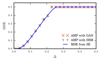
Figure 1: The MSE of the reconstruction of communities in the rank $r=2$ case. We present the result of AMP for two different channels the Gaussian additive noise (GAN, red crosses) and the stochastic block model (SBM, with $p_{\rm out}=0.5$, green crosses) compared to the theoretical value from the state evolution (SE, blue line). The AMP simulations were run on a single instance of size $n=20000$.

In figure 2 we depict the first order phase transition that occurs for $r>4$. We present the MSE obtained from density evolution as function of $r^{2}\Delta$ for various ranks $r=10,15,20$. From the uninformative initialization the MSE jumps to $1-1/r$ at $\Delta_{c}=1/r^{2}$. From the informative initialization the jump occurs at $\Delta_{\rm spinodal}>\Delta_{c}$ and by comparing the Bethe free energy of the two fixed points we evaluate the $\Delta_{\rm static}$. We observe that already for these values of the rank the gap between the information theoretical and computationally tractable performance, i.e. between $\Delta_{c}$ and $\Delta_{\rm static}$ is very large. Another interesting observation we made concerns the value of the MSE at the $\Delta_{c}=1/r^{2}$ transition. The reconstruction is very close to exact even at the phase transition itself. More precisely it decreases roughly exponentially with the rank $r$, being close to $10^{-10}$ for rank $r=100$.

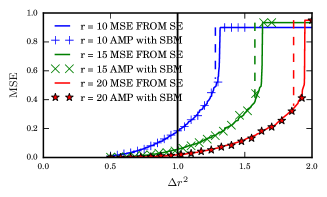
Figure 2: We plot MSE deduced from state evolution (lines) and from AMP (marks) for different values of rank $r$ as a function of $\Delta r^{2}$ (this rescaling is for visual reasons). The vertical full black line is $\Delta_{c}$ for all the cases. The vertical dashed colored lines are $\Delta_{\rm static}$ and the full lines correspond to the MSE obtained from the informative initializations and have discontinuities at $\Delta_{\rm spinodal}$.

In figure 3 we plot the values of $\Delta_{\rm spinodal}$ and $\Delta_{\rm static}$ rescaled by $r\log{r}$ as a function of the rank $r$. As the rank grows $r\to\infty$ the static line will converge to $1/4$ and the spinodal one to $1/2$ (59-60). Whereas the static transition converges nicely to its asymptotic value, for the spinodal transition we are still quite far from the asymptotic regime.

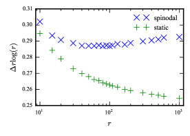
Figure 3: We plot $\Delta r\log{r}$ for the static and spinodal phase transitions obtained from the state evolution using the protocol described in Appendix C. We rescale the $\Delta$ in this way to compare with the large rank expansion in (59) and (60).

IV Conclusions and perspectives

We considered here the problem of estimation of a low rank matrix that was observed element-wise trough an arbitrary noisy channel. Using approximate message passing and its state evolution we compute the Bayes-optimal MMSE in this problem. The most interesting and, comparing to previously studied cases, surprising conclusion is that the MMSE depends on the output channel only trough its Fisher information.

As an example of the considered setting we study the problem of clustering in dense stochastic block model with the difference between probabilities of connection within and between communities scaling as $O(1/\sqrt{n})$. We evaluate the phase transitions and MMSE in this regime, unveiling a wide region of computational hardness.

Both the AMP algorithms and the state evolution apply to a number of other setting considered in the literature, which is a natural direction of future work.

V Acknowledgements

We thank Madhu Advani for clarifying discussion about Fisher information. The research leading to these results has received funding from the European Research Council under the European Union’s $7^{th}$ Framework Programme (FP/2007-2013)/ERC Grant Agreement 307087-SPARCS.

Appendix A

To derive the state evolution let us define

$$G_{il}=\frac{K}{\sqrt{n}}S_{il}{a_{l\rightarrow il}^{t}}.$$ (61)

We then have $B_{i}^{t}=\sum\limits_{l\neq i}G_{il}$. We use the central limit theorem to find the distribution of $B_{i}$ in order to do that one needs to compute, $\mathbb{E}_{Y}(G_{il})$ and ${\rm Cov}(G_{il}G_{ik}^{\top})$. Let us show how to compute the mean

$$\mathbb{E}(G_{il})=\int{\rm d}yP_{\rm out}\left(y|w_{il}\right)\frac{K}{\sqrt{n}}\frac{\partial g}{\partial w}\Big{|}_{y,0}{a_{l\rightarrow il}^{t}}.$$ (62)

We then expand the probability $P_{\rm out}(y|w)$ around 0

$$P_{\rm out}\left(y|w\right)=P_{\rm out}(y|0)\left(1+w\frac{\partial g}{\partial w}\Big{|}_{y,0}\right)\,.$$ (63)

Using (63) in (62) and using (16) and (16) we get

$$\mathbb{E}(G_{il})=\frac{K}{n\Delta}a_{j}x_{j}^{\top}Kx_{l}+O\left(n^{-\frac{3}{2}}\right)\,,$$ (64)

where $a_{i}$ is the mean of $a_{i\rightarrow il}$ with respect to $y_{ij}$. Using (63) and the fact that $a_{l\rightarrow il}$ and $a_{k\rightarrow ik}$ are independent random variables we can compute the second moments of the $G_{ij}$ as

$${\rm Cov}(G_{il},G_{ik})=\delta_{l}^{k}\frac{Ka_{i}a_{i}^{\top}K}{n\Delta},$$ (65)

From the central limit theorem we deduce.

$$B_{i}^{t}=\frac{KM^{t}K{x}_{i}}{\Delta}+W_{i}\,,$$ (66)

where $W_{i}$ is a Gaussian random variable of mean 0 and of covariance $KQ^{t}K/\Delta$.

Appendix B

The Bethe free energy in the case where all the factors are between two variables reads as

$$\Phi=n\phi=\sum\limits_{1\leq i\leq n}\mathbb{F}_{i}-\sum\limits_{1\leq i\leq j\leq n}\mathbb{F}_{ij}\,,$$ (67)

where

$$\mathbb{F}_{i}=\log\left[\int{\rm d}x_{i}P_{\rm prior}\prod_{j\neq i}m_{ij\rightarrow i}(x_{i})\right]$$ (68)

and

$$\mathbb{F}_{ij}=\log\left[\int{\rm d}x_{i}{\rm d}x_{j}P_{\rm out}\left(y_{ij}|w_{ij}\right)n_{i\rightarrow ij}(x_{i})n_{j\rightarrow ij}(x_{j})\right].$$ (69)

Using (6) we find

$$\sum\limits_{1\leq i\leq n}\mathbb{F}_{i}=\sum\limits_{i}\log{\cal Z}(A,B_{i})\,.$$ (70)

For the second term we expand once again $P_{\rm out}\left(y_{ij}|w_{ij}\right)$ around 0 and then take the mean with respect to each message. We then take the log and find

$$\mathbb{F}_{ij}=g(y_{ij},0)+\frac{a_{i\rightarrow ij}^{\top}Ka_{j\rightarrow ij}}{\sqrt{n}}S_{ij}-$$

$$\frac{S_{ij}^{2}}{2n}{\rm Tr}\left[Ka_{i\rightarrow ij}^{t}{a_{i\rightarrow ij}^{t}}^{\top}Ka_{j\rightarrow ij}^{t}{a_{j\rightarrow ij}^{t}}^{\top}\right]+$$

$$\frac{h(y_{ij})}{2n}{\rm Tr}\left[K\left(v_{l\rightarrow il}^{t}+a_{i\rightarrow ij}^{t}{a_{i\rightarrow ij}^{t}}^{\top}\right)\right.$$

$$\times\left.K\left(v_{l\rightarrow il}^{t}+a_{j\rightarrow ij}^{t}{a_{j\rightarrow ij}^{t}}^{\top}\right)\right]\,.$$ (71)

The TAPification procedure that is not detailed here gives us

$$a_{i\rightarrow ij}=a_{i}-\frac{S_{ij}a_{j}}{\sqrt{n}}+O\left(\frac{1}{n}\right)\,.$$ (72)

We also remove the term $g(y_{ij},0)$ since it is a constant that does not depend on the messages. We replace (72), (17) and (15) in (71) and we get

$$\mathbb{F}_{ij}=\frac{a_{i}^{\top}Ka_{j}}{\sqrt{n}}S_{ij}-\frac{1}{2n\Delta}{\rm Tr}\left[Ka_{i}^{t}{a_{i}^{t}}^{\top}Ka_{j}^{t}{a_{j}^{t}}^{\top}\right]\\ \frac{1}{\Delta n}{\rm Tr}\left[Ka_{i}a_{i}^{\top}Kv_{j}+Ka_{j}a_{j}^{\top}Kv_{i}\right]\,.$$ (73)

Since the sum is on all undirected links $ij$ we do the sum on all directed link and divide by $2$

$$\Phi=\sum\limits_{1\leq i\leq n}\log{\cal Z}(A,B_{i})-\\ \frac{1}{2}\sum\limits_{1\leq ij\leq n}\frac{a_{i}^{\top}Ka_{j}}{\sqrt{n}}S_{ij}-\frac{1}{2n\Delta}{\rm Tr}\left[Ka_{i}^{t}{a_{i}^{t}}^{\top}Ka_{j}^{t}{a_{j}^{t}}^{\top}\right]-\\ {\rm Tr}\left[\frac{K}{n\Delta}\left(\sum\limits_{1\leq i\leq n}a_{i}a_{i}^{\top}\right)K\left(\sum\limits_{1\leq i\leq n}v_{i}\right)\right]$$ (74)

To get the Bethe-free-energy in the large $n$ limit we compute the mean of $\frac{a_{i\rightarrow ij}^{\top}Ka_{j\rightarrow ij}}{\sqrt{n}}$ with respect to the noise. The main idea remains the same we compute the mean with respect to a perturbation of $P_{\rm out}$

$$\mathbb{E}\left(\frac{S_{ij}a_{i\rightarrow ij}^{\top}Ka_{j\rightarrow ij}}{\sqrt{n}}\right)=\\ \int{\rm d}yP_{\rm out}(y|0)\left(1+S_{ij}w_{ij}\right)\frac{S_{ij}a_{i\rightarrow ij}^{\top}Ka_{j\rightarrow ij}}{\sqrt{n}}$$ (75)

$$\mathbb{E}\left(\frac{S_{ij}a_{i\rightarrow ij}^{\top}Ka_{j\rightarrow ij}}{\sqrt{n}}\right)=\frac{Kx_{i}a_{i}^{\top}Ka_{j}x_{j}^{\top}}{n\Delta}\,.$$ (76)

To compute the mean of (70) we use the fact that we know the distribution of the $B_{i}$ (66). We replace (76) in (71) and we get

$$\phi =\mathbb{E}_{P_{x},P_{W}}\left[\log{\cal Z}(\frac{KQK}{\Delta},\frac{KMKx}{\Delta}+W)\right]$$ (77)

$$-\frac{1}{2\Delta}{\rm Tr}(KMKM^{\top})+\frac{1}{4\Delta}{\rm Tr}(KQKQ^{\top})\,.$$

Appendix C

To locate the phase transitions $\Delta_{\rm static}$ and $\Delta_{\rm spinodal}$ we make a couple of remarks about the state evolution. First we remark that for $\forall x\in\mathbb{R}^{+}$ $b={\cal M}_{r}(x)$ is a fixed point of (52) for $\Delta={{\cal M}_{r}(x)}/{x}$. By definition $\Delta_{\rm spinodal}$ is the greatest $\Delta$ for which $b_{\rm far}$ exist. Therefore

$$\Delta_{\rm spinodal}=\max_{x\in\mathbb{R}^{+}}\left\{\frac{{\cal M}_{r}(x)}{x}\right\}\,.$$ (78)

To find the $\Delta_{\rm static}$ one can notice that by taking the derivative with respect to $Q$ and $M$ of (30) one finds a combination of (28) and (29). Therefore we have

$$\phi(b_{2},\Delta)-\phi(b_{1},\Delta)=\frac{r-1}{2r^{2}\Delta}\int\limits_{b_{1}}^{b_{2}}{\rm d}u{\cal M}_{r}\left(\frac{u}{\Delta}\right)-u\,.$$ (79)

We deduce a way to compute $\Delta_{\rm static}$ as

$$\Delta_{\rm static}=\max_{x\in\mathbb{R}^{+}}\left\{\frac{{\cal M}_{r}(x)}{x},{\rm s.t.}\,\int\limits_{0}^{x}{\rm d}u{\cal M}_{r}(u)=\frac{x{\cal M}_{r}(x)}{2}\right\}\,.$$ (80)

To compute $\Delta_{\rm static}$ we evaluate ${\cal M}_{r}$ on a whole interval then for each $x$ draw a line between point $(0,0)$ and $(x,H(x))$. We then compute the area between ${\cal M}_{r}$ and this line. When this aera is zero then ${\cal M}_{r}(x)/{x}$ gives us $\Delta_{\rm static}$.

Appendix D

In this appendix we explain the derivation of (59), (60). To do this let us study the function ${\cal M}_{r}(x)$ where we take $x=\beta r\log(r)$, where $\beta=\Omega(1)$. The important part of ${\cal M}_{r}$ is this integral

$$\int\frac{\exp\left(\frac{x}{r}+u_{1}\right)}{\exp\left(\frac{x}{r}+u_{1}\right)+\sum\limits_{i=2}^{r}\exp\left(u_{i}\right)}\prod\limits_{i=1}^{r}{\cal D}u_{i}\,.$$ (81)

The important variables to look at are

$$F_{1}=\exp\left(\frac{x}{r}+u_{1}\right)\,,$$ (82)

$$F_{2}=\sum\limits_{i=2}^{r}\exp\left(u_{i}\right).$$ (83)

If $F_{1}$ dominates $F_{2}$ as $r\rightarrow+\infty$ then ${\cal M}_{r}=1$, otherwise if $F_{2}$ dominates $F_{1}$ then ${\cal M}_{r}=0$.

To estimate $F_{1}$, $F_{2}$ let us notice that with high probability the maximum value will be of order $\sqrt{2\beta\log(r)}$. This is a general property of Gaussian variables that the maximum of $r$ independent Gaussian variables of variance $\sigma^{2}$ is of order $\sigma\sqrt{2\log(r)}$. We can therefore compute the mean of $F_{2}$ all while conditioning on the fact that all of the $u_{i}$ are smaller than $\sqrt{2\beta\log(r)}$. This allows us to compute the typical value of $F_{1}$ as $F_{1}\sim r^{\beta}$. For $F_{2}$ we obtain: when $\beta<1/2$ then $F_{2}\sim r^{\beta+\frac{1}{2}}$, and when if $\beta>1/2$ then $F_{2}\sim r^{\sqrt{2\beta}}$. We have to look at which of the $F_{1}$ or $F_{2}$ has a higher exponent. In these computation we can therefore just assume that

$${\cal M}_{r}(\beta r\log(r))=\mathbb{1}\left(\beta>2\right)\,.$$ (84)

Now let us remind (78) while keeping $x=\beta r\log(r)$

$$\Delta_{\rm spinodal}=\max\left\{\frac{\mathbb{1}\left(\beta>2\right)}{\beta r\log(r)},\beta\in\mathbb{R}^{+}\right\}=\frac{1}{2r\log(r)}$$ (85)

To get the static transition we use (80). Let us find the $\beta$ that satisfies equation (80) we get

$$\beta r\log(r)\left[1-\frac{2}{\beta}\right]=\frac{\beta r\log(r)}{2}\,.$$ (86)

We deduce $\beta=4$ and therefore

$$\Delta_{\rm static}=\frac{1}{4r\log(r)}\,.$$ (87)

References

- [1] I. Carron, “The matrix factorization jungle,” https://sites.google.com/site/igorcarron2/matrixfactorizations.
- [2] Y. Deshpande and A. Montanari, “Information-theoretically optimal sparse PCA,” in Information Theory (ISIT), 2014 IEEE International Symposium on, 2014, pp. 2197–2201.
- [3] T. Lesieur, F. Krzakala, and L. Zdeborova, “Phase transitions in sparse PCA,” arXiv:1503.00338, 2015.
- [4] A. Mnih and R. Salakhutdinov, “Probabilistic matrix factorization,” in Advances in neural information processing systems, 2007, p. 1257.
- [5] D. L. Donoho, A. Maleki, and A. Montanari, “Message-passing algorithms for compressed sensing,” Proc. Natl. Acad. Sci., vol. 106, no. 45, pp. 18 914–18 919, 2009.
- [6] M. Bayati and A. Montanari, “The dynamics of message passing on dense graphs, with applications to compressed sensing,” IEEE Transactions on Information Theory, vol. 57, p. 764, 2011.
- [7] J. Wright, A. Ganesh, S. Rao, Y. Peng, and Y. Ma, “Robust principal component analysis: Exact recovery of corrupted low-rank matrices via convex optimization,” in Advances in neural information processing systems, 2009, pp. 2080–2088.
- [8] A. A. Shabalin, V. J. Weigman, C. M. Perou, and A. B. Nobel, “Finding large average submatrices in high dimensional data,” The Annals of Applied Statistics, pp. 985–1012, 2009.
- [9] Z. Ma, Y. Wu et al., “Computational barriers in minimax submatrix detection,” The Annals of Statistics, vol. 43, no. 3, p. 1089, 2015.
- [10] Y. Cheng and G. M. Church, “Biclustering of expression data.” in Ismb, vol. 8, 2000, pp. 93–103.
- [11] P. Gopalan, J. M. Hofman, and D. M. Blei, “Scalable recommendation with Poisson factorization,” arXiv preprint arXiv:1311.1704, 2013.
- [12] M. Lelarge, L. Massoulié, and J. Xu, “Reconstruction in the labeled stochastic block model,” in Information Theory Workshop (ITW), 2013 IEEE. IEEE, 2013, pp. 1–5.
- [13] S. Rangan and A. K. Fletcher, “Iterative estimation of constrained rank-one matrices in noise,” in Information Theory Proceedings (ISIT), 2012 IEEE International Symposium on. IEEE, 2012, pp. 1246–1250.
- [14] R. Matsushita and T. Tanaka, “Low-rank matrix reconstruction and clustering via approximate message passing,” in Advances in Neural Information Processing Systems, 2013, pp. 917–925.
- [15] S. Rangan, “Generalized approximate message passing for estimation with random linear mixing,” in IEEE International Symposium on Information Theory Proceedings (ISIT), 2011, pp. 2168 –2172.
- [16] Y. Kabashima, F. Krzakala, M. Mézard, A. Sakata, and L. Zdeborová, “Phase transitions and sample complexity in bayes-optimal matrix factorization,” arXiv preprint arXiv:1402.1298, 2014.
- [17] Y. Deshpande and A. Montanari, “Finding hidden cliques of size in nearly linear time,” Foundations of Computational Mathematics, pp. 1–60, 2015.
- [18] A. Decelle, F. Krzakala, C. Moore, and L. Zdeborová, “Asymptotic analysis of the stochastic block model for modular networks and its algorithmic applications,” Phys. Rev. E, vol. 84, no. 6, p. 066106, 2011.
- [19] R. R. Nadakuditi and M. E. Newman, “Graph spectra and the detectability of community structure in networks,” Physical review letters, vol. 108, no. 18, p. 188701, 2012.
- [20] Y. Deshpande, E. Abbe, and A. Montanari, “Asymptotic mutual information for the two-groups stochastic block model,” arXiv preprint arXiv:1507.08685, 2015.
- [21] M. Mézard and A. Montanari, Information, Physics, and Computation. Oxford: Oxford Press, 2009.
- [22] D. J. Thouless, P. W. Anderson, and R. G. Palmer, “Solution of ‘solvable model of a spin-glass’,” Phil. Mag., vol. 35, p. 593, 1977.
- [23] J. Vila, P. Schniter, S. Rangan, F. Krzakala, and L. Zdeborová, “Adaptive damping and mean removal for the generalized approximate message passing algorithm,” arXiv preprint arXiv:1412.2005, 2014.
- [24] J. Baik, G. Ben Arous, and S. Péché, “Phase transition of the largest eigenvalue for nonnull complex sample covariance matrices,” Annals of Probability, pp. 1643–1697, 2005.
- [25] D. Gross, I. Kanter, and H. Sompolinsky, “Mean-field theory of the Potts glass,” Physical review letters, vol. 55, no. 3, p. 304, 1985.
- [26] F. Caltagirone, G. Parisi, and T. Rizzo, “Dynamical critical exponents for the mean-field Potts glass,” Phys. Rev. E, vol. 85, no. 5, p. 051504, 2012.
- [27] F. Krzakala and L. Zdeborová, “Hiding quiet solutions in random constraint satisfaction problems,” Phys. Rev. Lett., vol. 102, p. 238701, 2009.