Itinerant electron scenario for Fe-based superconductors

Abstract

I review works on Fe-based superconductors which depart from a metal with well defined Fermi surfaces and Fermi liquid-type quasiparticles. I consider normal state instabilities – SDW magnetism and nematic order, and superconductivity, all three as the consequences of the instability of a Fermi surface due to interactions between low-energy fermionic quasiparticles. This approach assumes that renormalizations coming from fermions from high energies, of order bandwidth, modify but do not destroy Fermi liquid behavior in the normal state and can be absorbed into the effective low-energy model of interacting fermions located near hole and electron-type Fermi surfaces. I argue that the interactions between these fermions are responsible for (i) a stripe-type SDW magnetic order (and, in some special cases, a checkerboard order ) , (ii) a pre-emptive nematic-type instability, in which magnetic fluctuations break $C_{4}$ lattice rotational symmetry down to $C_{2}$, but magnetic order does not yet develop, and (iii) a superconductivity, which competes with these two orders. The experimental data on superconductivity show very rich behavior with potentially different symmetry of a superconducting state even for different compositions of the same material. I argue that, despite all this, the physics of superconductivity in the itinerant scenario for Fe-based materials is governed by a single underlying pairing mechanism.

I Introduction

The discovery of superconductivity in $Fe$-based pnictides [bib:Hosono, ] (Fe-based compounds with elements from the 5th group: N, P, As, Sb, Bi) was, arguably, among the most significant breakthroughs in condensed matter physics during the past decade. A lot of efforts by the condensed-matter community have been devoted in the few years after the discovery to understand normal state properties of these materials, the pairing mechanism, and the symmetry and the structure of the pairing gap.

The family of $Fe$-based superconductors (FeSCs) is already quite large and keeps growing. It includes various Fe-pnictides such as $1111$ systems RFeAsO ($R=$rare earth element) [bib:Hosono, ; bib:X Chen, ; bib:G Chen, ; bib:ZA Ren, ], $122$ systems XFe₂As₂(X=alkaline earth metals) [bib:Rotter, ; bib:Sasmal, ; bib:Ni, ], 111 systems like LiFeAs [bib:Wang, ], and also Fe-chalcogenides (Fe-based compounds with elements from the 16th group: S, Se, Te) such as FeTe_1-xSe_x   [bib:Mizuguchi, ] and A_xFe_2-ySe₂ ($A=K,Rb,Cs$)  [exp:AFESE, ; exp:AFESE_ARPES, ].

Superconductivity (SC) in FeSCs emerges upon either hole or electron doping (see Fig. 1), but can also be induced by pressure or by isovalent replacement of one pnictide element by another, e.g., As by P (Ref. [nakai, ]). In some systems, like LiFeAs  [bib:Wang, ], LiFeP [bib_mats_1, ] and LaFePO  [bib:Kamihara, ], SC emerges already at zero doping, instead of a magnetic order.

Parent compounds of nearly all FeSCs are metals, in distinction to cuprate superconductors for which all parent compounds are Mott insulators. Still, in similarity with the cuprates, in most cases these parent compounds are antiferromagnetically ordered  [Cruz, ]. Some researchers [localized, ; loc_sel, ; loc_it, ] used this analogy to argue that FeSCs are at short distance from Mott transition, and at least some elements of Mott physics must be included into the description of these systems. A rather similar point of view is [loc_it, ] that fermionic excitations in FeSCs display both localized and itinerant properties and the interplay between the two depends on the type of the orbital (one set of ideas of this kind lead to the notion of "orbital selective Mott transition on FeSCs [loc_sel, ; loc_it, ]). An alternative point of view, which I will present in this review, is that low-energy properties of most of FeSCs can be fully captured in a itinerant approach, without invoking Mott physics.

In itinerant approach, electrons, which carry magnetic moments, travel relatively freely from site to site. The magnetic order of such electrons is often termed as a spin-density-wave (SDW), by analogy with e.g., antiferromagnetic $Cr$, rather than "Heisenberg antiferromagnetism" – the latter term is reserved for systems in which electrons are "nailed down" to particular lattice sites by very strong Coulomb repulsion. From experimental perspective, the majority of FeSCs display a rather small ordered moment in the normal state, consistent with SDW scenario [review, ]. There are notable exceptions – Fe-chalcogenide FeTe (the parent compound of FeTe_1-xSe_x, which superconduct at $x$ around $0.5$) displays magnetic properties consistent with the Heisenberg antiferromagnetism of localized spins [Zaliznyak12, ]. However, the properties of this material vary quite substantially between $x=0$ and $x=0.5$, and magnetic fluctuations at $x\sim 0.5$ are similar to those of other FeSCs. Another example where magnetism is strong and probably involves localized carriers is A_xFe_2-ySe₂ (Ref. [exp:AFESE, ]). However, in this material, localized carriers and itinerant carriers are most likely phase separated, with superconductivity coming primarily from itinerant carriers.

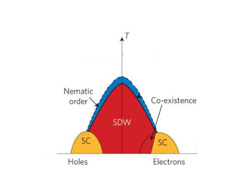
Figure 1: Schematic phase diagram of Fe-based pnictides upon hole or electron doping. In the shaded region, superconductivity and antiferromagnetism co-exist. Not all details/phases are shown. Superconductivity can be initiated not only by doping but also by pressure and/or isovalent replacement of one pnictide element by another  [nakai, ]. Nematic phase at $T>T_{N}$ is subject of debates. Superconductors at large doping are KFe₂As₂ for hole doping   [KFeAs_ARPES_QO, ; KFeAs_exp_nodal, ] and A_xFe_2-ySe₂ (A = K, Rb, Cs) for electron doping  [exp:AFESE, ; exp:AFESE_ARPES, ]. Whether superconductivity in pnictides exists at all intermediate dopings is not clear yet. From Ref. [review_we, ].

The itinerant approach to magnetism and superconductivity in FeSCs and the comparative analysis of Fe- and Cu-based superconductors have been reviewed in several recent publications  [review, ; review_2, ; review_3, ; review_4, ; Graser, ; peter, ; Kuroki_2, ; rev_physica, ; mazin_schmalian, ; review_we, ; korshunov, ; ch_annual, ; maiti_rev, ]. This review is an attempt to summarize our current understanding of the phase diagram, the origin of SDW and nematic orders, the pairing mechanism for superconductivity, and the symmetry and the structure of the pairing gap at various hole and electron dopings.

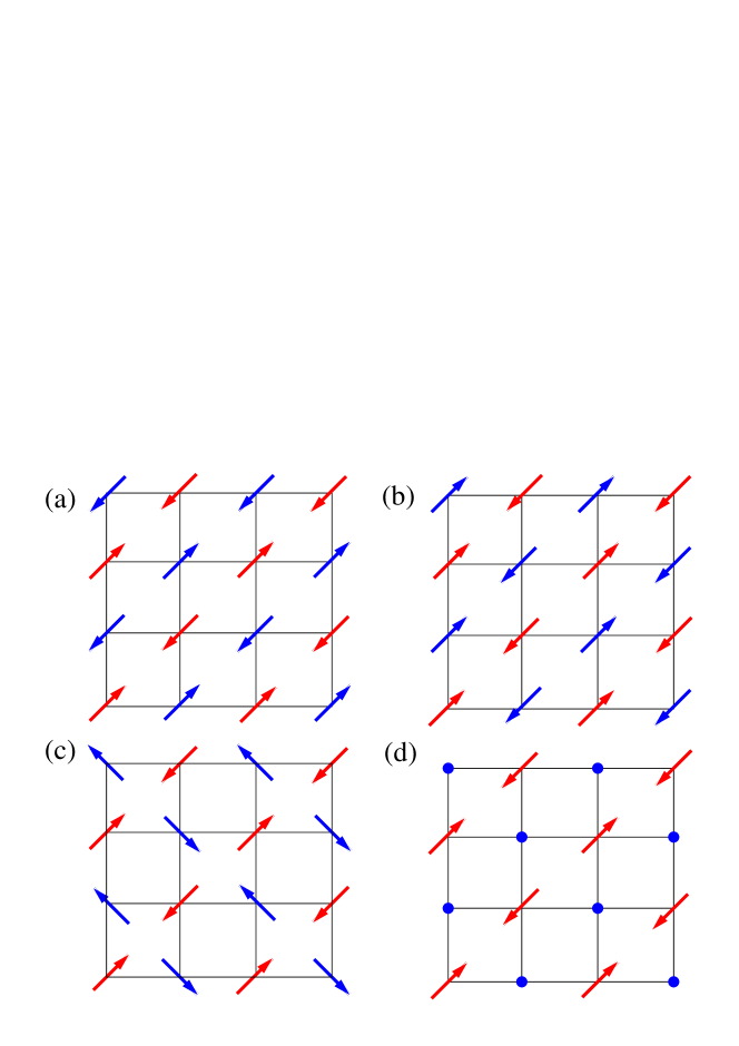
Figure 2: (color online) Various SDW spin configurations described by $\vec{\Delta}_{1}e^{i{\bf Q}_{1}R}+\vec{\Delta}_{2}e^{i{\bf Q}_{2}R}$. For a perfect nesting only $\vec{\Delta}^{2}_{1}+\vec{\Delta}^{2}_{2}$ is fixed. Panel (a) – $\vec{\Delta}_{1}=0$, panel (b) – $\vec{\Delta}_{2}=0$, panel (c) – $\vec{\Delta}_{1}\perp\vec{\Delta}_{2}$, and panel (d) – $\vec{\Delta}_{1}=\vec{\Delta}_{2}$. From [Eremin_10, ]

.

Like I said, the very idea of itinerant approach is that magnetism and superconductivity come from the interactions between fermionic states located very near the Fermi surfaces. These interactions originate from a Coulomb interaction, which is obviously a repulsive one.

A repulsive interaction between itinerant carriers is well known to lead to Stoner-type magnetic instability, and the presence of the SDW-ordered phase on the phase diagram of FeSCs should not come as a surprise. Less obvious issue is what kind of magnetism is present in FeSCs. Experiments show that most of undoped and weakly doped Fe-pnictides display the stripe spin-density wave order at $T<T_{sdw}$, with ordering vectors $(0,\pi)$ or $(\pi,0)$ in the 1-Fe Brillouin zone (1FeBZ), Ref.[Yildirim08, ; Xiang08, ] (see Fig. 2). Such an order not only breaks $O(3)$ spin symmetry, but also breaks lattice rotational symmetry from $C_{4}$ down to $C_{2}$ (the stripes run either along $X$ or along $Y$ direction). Stripe, order, however, does not emerge in all cases. Neutron scattering data on more heavily doped Ba_1-xNa_xFe₂As₂ (Ref. [ osborn, ]) and on Ba(Fe_1-xMn_x)₂As₂  (Ref. [rafael_last, ]) show that the magnetic order there does not break $C_{4}$ symmetry (examples are shown in Fig. 2). I will argue that both types of magnetic order (the one which breaks $C_{4}$ symmetry and the one which doesn’t) emerge in the itinerant scenario for FeSCs.

Another interesting aspect of the normal state phase diagram is that in weakly doped Fe-pnictides, the stripe SDW order is often preceded by a “nematic” phase with broken $C_{4}$ tetragonal symmetry but unbroken $O(3)$ spin rotational symmetry. The emergence of such a phase is not only manifested by a tetragonal to orthorhombic transition at $T_{n}\geq T_{sdw}$, but also by the onset of significant anisotropies in several quantities [Fisher11, ], such as dc resistivity [Chu10, ; Tanatar10, ], optical conductivity [Duzsa11, ; Uchida11, ], local density of states [Davis10, ], orbital occupancy [Shen11, ], susceptibility [Matsuda11, ], and the vortex core in the mixed superconducting state [Song11, ]. The fact that the SDW and structural transition lines follow each other across all the phase diagrams of 1111 and 122 materials, even inside the superconducting dome [FernandesPRB10, ; Nandi09, ], prompted researchers to propose that SDW and nematic orders are intimately connected. The interplay between magnetic and structural transitions in FeSCs is also quite rich: while in 1111 materials the two transitions are second-order and split ($T_{n}>T_{cdw}$), in most of the 122 materials they seem to occur simultaneously or near-simultaneously at small dopings, but clearly split above some critical doping - $x\approx 0.022$ in $\mathrm{Ba\left(Fe_{1-\mathit{x}}Co\mathit{{}_{x}}\right)_{2}As_{2}}$, see [Kim11, ; Birgeneau11, ], and $x\approx 0.039$ in $\mathrm{Ca\left(Fe_{1-\mathit{x}}Co\mathit{{}_{x}}\right)_{2}As_{2}}$, see [Prokes11, ].

For superconductivity, the central issue is what causes the attraction between fermions. The BCS theory of superconductivity attribute the attraction between fermions to the underlying interaction between electrons and phonons  [BCS, ] (the two electrons effectively interact with each other by emitting and absorbing the same phonon which then serves as a glue which binds electrons into pairs). Electron-phonon mechanism has been successfully applied to explain SC in a large variety of materials, from $Hg$ and $Al$ to recently discovered and extensively studied $MgB_{2}$ with the transition temperature $T_{c}=39K$  [mgb2, ]. However, for FeSCs, early first-principle study of superconductivity due to electron-phonon interaction placed $T_{c}$ at around $1K$, much smaller that the actual $T_{c}$ in most of FeSCs. This leaves an electron-electron interaction as the more likely source of the pairing.

Pairing due to electron-electron interaction has been discussed even before high $T_{c}$ era, most notably in connection with superfluidity in ${}^{3}He$  [3he, ; 3he2, ], but became the mainstream after the discovery of SC in the cuprates [bednortz, ]. This discovery signaled the beginning of the new era of “high-temperature superconductivity” to which FeSCs added a new avenue with quite high traffic over the last five years.

A possibility to get superconductivity from nominally repulsive electron-electron interaction is based on two fundamental principles. First, in isotropic systems the analysis of superconductivity factorizes [stat_phys, ] between pairing channels with different angular momenta $l=0,1,2,3$, etc [in spatially isotropic systems $l=0$ component is called $s-$wave, $l=1$ component is called $p-$wave, $l=2$ component is called $d-$wave, and so on]. If just one component with some $l$ is attractive, the system undergoes a SC transition at some temperature $T=T_{c}$. Second, the screened Coulomb interaction $U(r)$ is constant and repulsive at short distances, but oscillates at large distances and may develop an attractive component at some $l$. Kohn and Luttinger (KL) have explicitly proven back in 1965 (Ref.  [KL, ]) that the combination of these two effects necessary leads to a pairing instability, at least at large odd $l$, no matter what the form of $U(r)$ is.

In lattice systems, angular momentum is no longer a good quantum number, and the equation for $T_{c}$ only factorizes between different irreducible representations of the lattice space group. In tetragonal systems, which include both cuprates and FeSCs , there are four one-dimensional irreducible representations $A_{1g}$, $B_{1g}$, $B_{2g}$, and $A_{2g}$ and one two-dimensional representation $E_{2g}$. Each representation has infinite set of eigenfunctions. The eigenfunctions from $A_{1g}$ are invariant under symmetry transformations in a tetragonal lattice: $x\to-x,\leavevmode\nobreak\ y\to-y,\leavevmode\nobreak\ x\to y$, the eigenfunctions from $B_{1g}$ change sign under $x\to y$, and so on. If a superconducting gap has $A_{1g}$ symmetry, it is often called $s-$wave because the first eigenfunction from $A_{1g}$ group is just a constant in momentum space (a $\delta-$function in real space). If the gap has $B_{1g}$ or $B_{2g}$ symmetry, it is called $d-$wave ($d_{x^{2}-y^{2}}$ or $d_{xy}$, respectably), because in momentum space the leading eigenfunctions in $B_{1g}$ and $B_{2g}$ are $\cos k_{x}-\cos k_{y}$ and $\sin k_{x}\sin k_{y}$, respectively, and these two reduce to $l=2$ eigenfunctions $\cos 2\theta$ and $\sin 2\theta$ in the isotropic limit.

In the cuprates, the superconducting gap has been proved experimentally to have $B_{1g}$ symmetry  [d-wave, ]. Such a gap appears quite naturally in the doping range where the cuprates are metals, because KL-type consideration shows that $B_{1g}$ interaction becomes attractive if the fully dressed repulsive interaction between fermions near different corners of the Brillouin zone (the one at momentum transfer near $(\pi,\pi)$) exceeds the repulsion at small momentum transfer. The enhancement of $(\pi,\pi)$ interaction is a sure thing if the system displays strong antiferromagnetic spin fluctuations (see Fig.3). That $B_{1g}$ gap is selected is not a surprise because such gap $\Delta(k)\propto cosk_{x}-\cos k_{y}$ changes sign not only under $k_{x}\to k_{y}$ but also between ${\bf k}$ and ${\bf k}^{\prime}={\bf k}+{\bf Q}$ where ${\bf Q}=(\pi,\pi)$. This sign change is the crucial element for any electronic mechanism of superconductivity because one needs to extract an attractive component from repulsive screened Coulomb interaction.

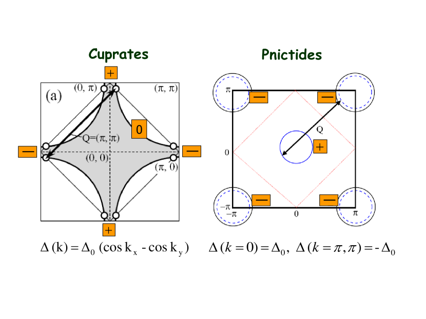
Figure 3: A comparison of the pairing state from spin-fluctuation exchange in cuprate SCs and in FeSCs. In the cuprates (left panel) the FS is large, and antiferromagnetic ${\bf Q}=(\pi,\pi)$ connects points on the same FS. Because spin-mediated interaction is positive (repulsive), the gap must change sign between FS points separated by ${\bf Q}$. As the consequences, the gap changes sign twice along the FS. This implies a $d-$wave gap symmetry. In FeSCs (left panel) scattering by ${\bf Q}$ moves fermions from one FS to the other. In this situation, the gap must change sign between different FS, but to first approximation remains a constant on a given FS. By symmetry, such a gap is an $s-$wave gap. It is called $s^{+-}$ because it changes sign between different FSs

In FeSCs, magnetism and superconductivity are also close neighbors on the phase diagram, and it has been proposed  [Mazin, ; Kuroki, ] at the very beginning of the $Fe$ era that the pairing mechanism in FeSCs is also a spin-fluctuation exchange. However, the geometry of low-energy states in FeSCs and in the cuprates is different, and in most FeSCs the momentum ${\bf Q}$ connects low-energy fermionic states near the center and the corner of the Briilouin zone (see Fig.3). A simple experimentation with trigonometry then tell us that the SC order parameter (the gap) $\Delta(k)$ must be symmetric with respect to $k_{x}\to k_{y}$ and $k_{x}\to-k_{x}$, but still must change sign under ${\bf k}\to{\bf k}+{\bf Q}$. Such order parameter belongs to $A_{1g}$ representation, but it only has contributions from a particular subset of $A_{1g}$ states with the form $\cos k_{x}+\cos k_{y}$, $\cos{3k_{x}}+\cos(3k_{y})$, etc, which all change sign under ${\bf k}\to{\bf k}+{\bf Q}$. An order parameter with such symmetry is called an extended $s-$wave or, in shorter notations, $s^{+-}$.

Majority of researches do believe that in weakly/moderately doped FeSCs the gap does have $s^{+-}$ symmetry. However, numerous studies of superconductivity in FeSCs over the last five years demonstrated that the physics of the pairing is more involved than it was originally thought because of multi-orbital/multi-band nature of low-energy fermionic excitations in FeSCs. It turns out that both the symmetry and the structure of the pairing gap result from rather non-trivial interplay between spin-fluctuation exchange, intraband Coulomb repulsion, and momentum structure of the interactions. In particular, an $s^{\pm}$ gap can be with or without nodes, depending on the orbital content of low-energy excitations. Besides, the structure of low-energy spin fluctuations evolves with doping, and the same spin-fluctuation mechanism that gives rise to $s^{+-}$ gap at small/moderate doping in a particular material can give rise to a $d-$wave gap at strong hole or electron doping.

There is more uncertainly on the theory side. In addition to spin fluctuations, FeSCs also possess charge fluctuations whose strength is the subject of debates. There are proposals  [jap, ; ku, ] that in multi-orbital FeSCs charge fluctuations are strongly enhanced because the system is reasonably close to a transition into a state with an orbital order – a spontaneous symmetry breaking between the occupation of different orbitals). (A counter-argument is that orbital order does not develop on its own but is induced by a magnetic order [rafael_nematic, ; rafael_review, ]). If charge fluctuations are relevant, one should consider, in addition to spin-mediated pairing interaction, also the pairing interaction mediated by charge fluctuations. The last interaction gives rise to a conventional, sign-preserving $s-$wave pairing  [jap, ]. A "p-wave" gap scenario (a gap belonging to $E_{2g}$ representation) has also been put forward  [p_lee, ].

From experimental side, $s$-wave gap symmetry is consistent with ARPES data on moderately doped B_1-xK_x Fe₂As₂ and BaFe₂(As_1-xP_x)₂, which detected only a small variation of the gap along the FSs centered at $(0,0)$ (Ref. [laser_arpes, ]), and with the evolution of the tunneling data in a magnetic field  [hanaguri, ]. However, other data on these and other FeSCs, which measure contributions from all FSs, including the FSs for which ARPES data are not available at the moment, were interpreted as evidence either for the full gap  [ding, ; chen, ; osborn1, ; carrington1, ], or that the gap has either accidental nodes  [nodes, ; carrington, ] or deep minima  [proz, ; proz_1, ; moler, ]. As additional level of complexity, superconductivity was also discovered in materials which only contain hole pockets, like hole-doped KFe₂As₂, or only electron pockets, like A_xFe_2-ySe₂ . For these materials, the argument for $s^{+-}$ superconductivity, driven by magnetically-enhanced interaction between fermions near hole and electron pockets, is no longer applicable, yet both classes of materials have finite $T_{c}$, which is around 3K for KFe₂As₂  and as high as 30K for A_xFe_2-ySe₂   (Refs. [Guo2010, ]). For KFe₂As₂, Various experimental probes  [KFeAs_exp_nodal, ] indicate the presence of gap nodes. Laser ARPES data [shin, ] were interpreted as evidence for $s-$wave with nodes, while thermal conductivity data have been interpreted as evidence for both, $d-$wave and $s-$wave orders (Refs.[reid, ] and [mats_2, ], respectively). For A_xFe_2-ySe₂ , ARPES results were interpreted as evidence for $s-$wave (Ref.[exp:AFESE_ARPES, ]), however neutron scattering experiments [AFESE_neu, ] detected a resonance peak which most naturally can be interpreted as evidence for $d-$wave [AFESE_d, ] (see, however, [khodas_2, ]).

In this paper, I argue that all these seemingly very different gap structures actually follow quite naturally from the same underlying physics idea that FeSCs can be treated as moderately interacting itinerant fermionic systems with multiple FS sheets and effective four-fermion intra-band and inter-band interactions in the band basis. I introduce the effective low-energy model with small numbers of input parameters  [maiti_11, ] and use it to study the doping evolution of the pairing in hole and electron-doped FeSCs. I argue that various approaches based on underlying microscopic models in the orbital basis reduce to this model at low energies.

The paper is organized as follows. In Sec. II I discuss general aspects of the band structure of FeSCs which contain hole and electron pockets. In Sec. III I present a generic discussion of what is needed for SDW order and superconductivity and how magnetic fluctuations help superconductivity to develop. In Sec. IV I briefly review parquet renormalization group approach to FeSCs. This approach treats magnetism and superconductivity on equal footing. I argue that, depending on input parameters and/or doping, the system first becomes either SDW magnet or a superconductor. In Sec.VI I review itinerant approach to magnetism. I show that for most (but not all) dopings a SDW order below $T_{sdw}$ spontaneously breaks $C_{4}$ lattice symmetry in addition to $O(3)$ symmetry of rotations in spin space. I then review works on a pre-emptive spin-nematic instability at $T_{n}>T_{sdw}$, when the system spontaneously breaks $C_{4}$ symmetry down to $C_{2}$, but spin-rotational symmetry remains unbroken down to a smaller $T_{sdw}$. In Sec.VII I review an itinerant approach to superconductivity. I first present a generic symmetry consideration of a gap structure in a multi-band superconductor and show that a “conventional wisdom” that an s-wave gap is nodeless along the FSs, d-wave gap has four nodes, etc, has only limited applicability in multi-band superconductors, and there are cases when the gap with nodes has an $s-$wave symmetry, and the gap without nodes has a $d-$wave symmetry. I then discuss the interplay between intra-band and inter-band interactions, for realistic multi-pocket models for FeSCs and set the conditions for an attraction in an $s-$wave or a $d-$wave channel. I consider 5-orbital model with local interactions, convert it into a band basis, and show the structure of the superconducting gap. I use the combination of RPA and leading angular harmonic approximation to analyze the pairing in $s-$ and $d-$wave channels at different dopings. I show that, depending on parameters and doping, magnetically-mediated pairing leads to an $s^{\pm}$ superconductivity with either a near constant gap along the FSs, or gaps with deep minima, or even with the nodes. I briefly review the experimental situation in Sec. VIII and present concluding remarks in Sec. IX.

II The electronic structure of FeSCs.

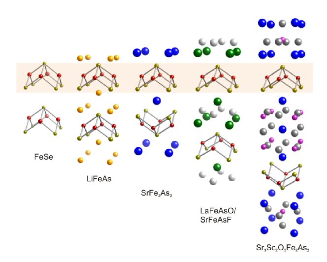
Figure 4: Crystallographic structures of various families of iron-based superconductors. From Ref.  [review_2, ].

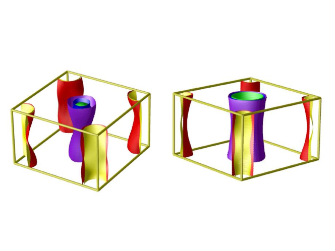
Figure 5: The electronic structure of FeSCs. In weakly and moderately electron-doped materials (left panel) the FS consists of quasi-2D warped cylinders centered at $(0,0)$ and $(\pi,\pi)$ in a 2D cross-section. The ones near $(0,0)$ are hole pockets (filled states are outside cylinders), the ones near $(\pi,\pi)$ are electron pockets (filled states are inside cylinders) There also exists a quasi-3D hole pocket near $k_{z}=\pi$. In hole-doped FeSCs the electronic structure is very similar, but 3D hole pocket becomes quasi-2D warped hole cylinder. From Ref.  [mazin_schmalian, ].

The crystallographic structures of various families of iron-based superconductors is shown in Fig. 4. All FeSCs contain planes made of Fe atoms, and pnictogen/chalcogene atoms are staggered in a checkerboard order above and below the iron planes. In 1111 system this order repeats itself from one Fe plane to the other, while for 122-type systems, it flips sign between neighboring planes.

The electronic structures of FeSCs at low energies are rather well established by ARPES [Li, ] and quantum oscillation measurements  [bib:Suchitra, ]. In weakly and moderately electron-doped materials, like BaFe_1-xCo_xFe₂As₂ the FS contains several quasi-2D warped cylinders centered at $k=(0,0)$ and $k=(\pi,\pi)$ in a 2D cross-section, and may also contain a quasi-3D pocket near $k_{z}=\pi$ (Fig.5). The fermionic dispersion is electron-like near the FSs at $(\pi,\pi)$ (filled states are inside a FS) and hole-like near the FSs centered at $(0,0)$ (filled states are outside a FS). In heavily electron-doped FeSCs, like A_xFe_1-ySe₂ (A = K, Rb, Cs), only electron pockets remain, according to recent ARPES studies.  [exp:AFESE, ] In weakly and moderately hole-doped FeSCs, like Ba_1-xK_xFe₂As₂, the electronic structure is similar to that at moderate electron doping, however the spherical FS becomes the third quasi 2D hole FS centered at $(2\pi,0)=(0,0)$. In addition, new low-energy hole states likely appear around $(\pi,\pi)$ and squeeze electron pockets  [Evtush, ]. At strong hole doping, electron FSs disappear and only only hole FSs are present  [KFeAs_ARPES_QO, ] These electronic structures agree well with first-principle calculations   [bib:first, ; Boeri, ; review_3, ], which is another argument to treat FeSCs as itinerant fermionic systems.

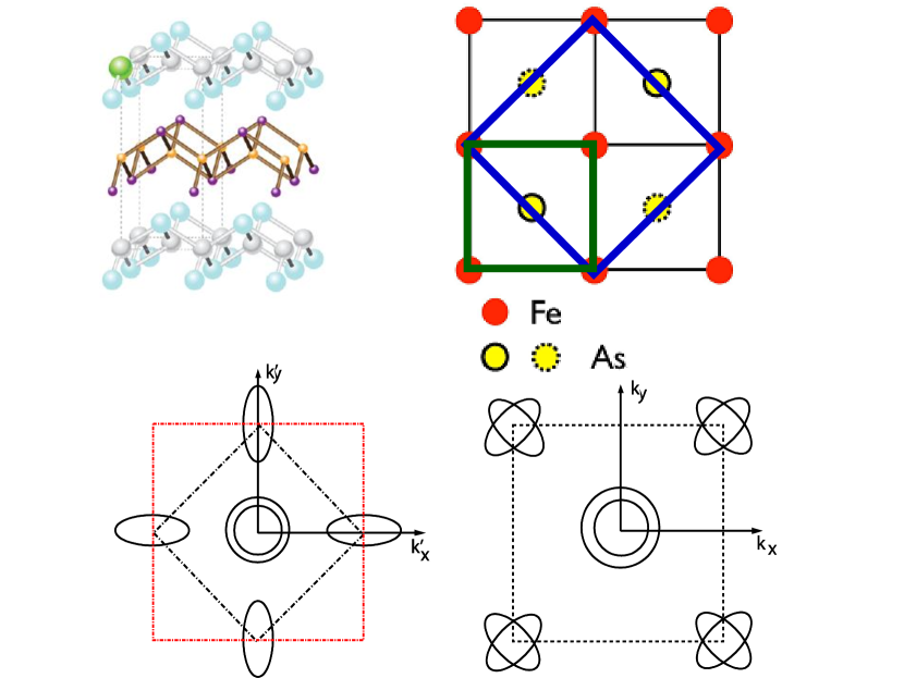
Figure 6: Upper panel: 3D electronic structure of LaOFeAs (left) and its 2D cross-section (left). In only Fe states are considered, an elementary cell contains one Fe atom (green). The actual unit cell (blue) contains two Fe atoms because of two non-equivalent positions of a pnictide above and below the Fe plane. Lower panel – the location of hole and electron FSs in a 2D cross section in the folded BZ (two Fe/cell, right) and in the unfolded BZ (one Fe/cell, left). From Refs.  [norman, ],  [ising, ](b) and  [vekhter_10, ]b.

The measured FS reflects the actual crystal structure of FeSCs in which there are two non-equivalent positions of a pnictide above and below an $Fe$ plane, and, as a result, there are two $Fe$ atoms in the unit cell (this actual 2Fe BZ is called "folded BZ"). From theory perspective, it would be easier to work in the BZ which contains only one $Fe$ atom in the unit cell (this theoretical 1Fe BZ is called "unfolded BZ"). I illustrate the difference between folded and unfolded BZ in Fig.6. In general, only folded BZ is physically meaningful. However, if by some reason a potential from a pnictogen (or chalcogen) can be neglected, the difference between the folded and the unfolded BZ becomes purely geometrical: the momenta ${\tilde{k}}_{x}$ and ${\tilde{k}}_{y}$ in the folded BZ are linear combinations of $k_{x}$ and $k_{y}$ in the unfolded BZ: ${\tilde{k}}_{x}=k_{x}+k_{y}$, ${\tilde{k}}_{y}=k_{x}-k_{y}$. In this situation, the descriptions in the folded and unfolded BZ become equivalent.

Most of the existing theory works on magnetism and on the pairing mechanism and the structure of the SC gap analyze the pairing problem in the unfolded BZ, where which two hole pockets are centered at $(0,0)$ and one at $(\pi,\pi)$, and the two electron pockets are at $(0,\pi)$ and $(\pi,0)$. It became increasingly clear recently that the interaction via a pnictogen/chalcogen and also 3D effects do play some role for the pairing, particularly in strongly electron-doped systems.  [3D, ; mazin, ] However, it is still very likely that the key aspects of the pairing in FeSCs can be understood by analyzing a pure 2D electronic structure with only Fe states involved. In the next three sections I assume that this is the case and consider a 2D model in the unfolded BZ with hole FSs near $(0,0)$ and $(\pi,\pi)$ and electron FSs at $(0,\pi)$ and $(\pi,0)$.

III The low-energy model and the interplay between magnetism and superconductivity

For proof-of-concept I first consider a simple problem: a 2D two-pocket model with one hole and one electron FS, both circular and of equal sizes (see Fig.7), and momentum-independent four-fermion interactions.

The free-fermion Hamiltonian is the sum of kinetic energies of holes and electrons:

$$H_{2}=\sum_{k,\sigma}{\varepsilon}_{c}c^{{\dagger}}_{k,\sigma}c_{k,\sigma}+{\varepsilon}_{f}f^{{\dagger}}_{k,\sigma}f_{k,\sigma}$$ (1)

where $c$ stands for holes, $f$ stands for electrons, and ${\varepsilon}_{c,f}$ stand for their respective dispersions with the property that ${\varepsilon}_{c}(k)=-{\varepsilon}_{f}(k+Q)$, where $\textbf{Q}=(\pi,\pi)$ is the momentum vector which connects the centers of the two fermi surfaces. The density of states $N_{0}$ is the same on both pockets, and the electron pocket ‘nests’ perfectly within the hole pocket when shifted by Q.

There are five different types of interactions between low-energy fermions: two intra-pocket density-density interactions, which I treat as equal, interaction between densities in different pockets, exchange interaction between pockets, and pair hopping term, in which two fermions from one pocket transform into two fermions from the other pocket. I show these interactions graphically in Fig 8.

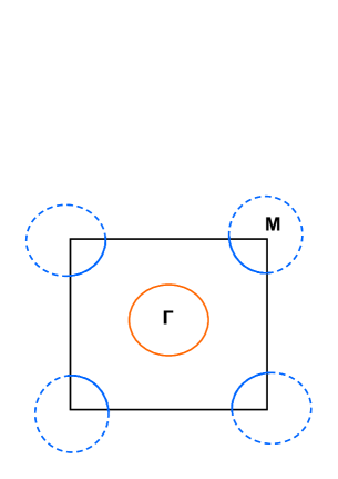
Figure 7: FS topology for a two-pocket model for FeSCs. The two FSs are for hole-like dispersion (blue circle, filled states outside the FS) and electron-like dispersion (orange circle, filled states inside the FS).

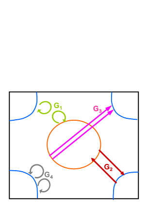
Figure 8: The interactions between pockets in the two-pocket model for Fe-pnictides. $G_{1}$ is a density-density interaction between fermions from different pockets. $G_{2}$ is an exchange interaction between the pockets, $G_{3}$ is a pair hopping process between the pockets, and $G_{4}$ is a density-density interaction within the same pocket. All interactions are repulsive (positive). From [maiti_rev, ; maiti_book, ].

In explicit form

$$H_{\text{int}} = G_{1}\sum_{[k,\sigma]}c^{\dagger}_{k_{1}\sigma}f^{\dagger}_{k_{2}\sigma^{\prime}}f_{k_{3}\sigma^{\prime}}c_{k_{4}\sigma}$$

$$+G_{2}\sum_{[k,\sigma]}f^{\dagger}_{k_{1}\sigma}c^{\dagger}_{k_{2}\sigma^{\prime}}f_{k_{3}\sigma^{\prime}}c_{k_{4}\sigma}$$

$$+\sum_{[k,\sigma]}\frac{G_{3}}{2}\left(c^{{\dagger}}_{k_{1},\sigma_{1}}c^{{\dagger}}_{k_{2},\sigma_{2}}f_{k_{3},\sigma_{2}}f_{k_{4},\sigma_{1}}+\text{h.c}\right)$$

$$+\sum_{[k,\sigma]}\left(\frac{G_{4}}{2}c^{{\dagger}}_{k_{1},\sigma_{1}}c^{{\dagger}}_{k_{2},\sigma_{2}}c_{k_{3},\sigma_{2}}c_{k_{4},\sigma_{1}}+c\leftrightarrow f\right)$$

where $\sum{{}_{[k,\sigma]}}$ is short for the sum over the spins and the sum over all the momenta constrained to $k_{1}+k_{2}=k_{3}+k_{4}$ modulo a reciprocal lattice vector.

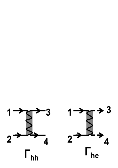
Figure 9: Vertices $\Gamma_{hh}=\Gamma_{ee}$ and $\Gamma_{he}$ introduced in the 2 pocket model. Solid and dashed lines denote fermions from the two pockets. From [cee, ].

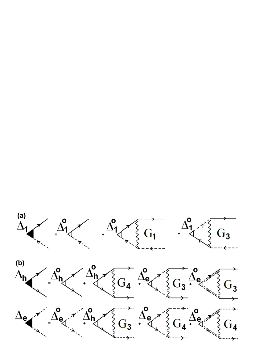
Figure 10: Lowest-order terms in the ladder series for the renormalizations of the SDW and superconducting vertices. The effective coupling in the SDW channel is $G_{1}+G_{3}$. The two couplings in the two SDW channels are $G_{3}+G_{4}$ and $-G_{3}+G_{4}$. From [maiti_rev, ; maiti_book, ].

The textbook approach to analyse potential instabilities towards superconductivity and magnetism is to consider the appearance of the poles in the corresponding vertex functions. For superconductivity, we need to consider vertex functions with zero total incoming momentum: $\Gamma_{hh}({\bf k}_{F},-{\bf k}_{F};{\bf p}_{F},-{\bf p}_{F});\Gamma_{ee}({\bf k}_{F},-{\bf k}_{F};{\bf p}_{F},-{\bf p}_{F})$, where ${\bf k}_{F}$ and ${\bf p}_{F}$ belong to the same pocket, and $\Gamma_{he}({\bf k}_{F},-{\bf k}_{F};{\bf p}_{F},-{\bf p}_{F})$, where ${\bf k}_{F}$ and ${\bf p}_{F}$ belong to different pockets (see Fig. 9). To first order in $G_{i}$, we have

$$\Gamma^{0}_{hh}({\bf k}_{F},-{\bf k}_{F};{\bf p}_{F},-{\bf p}_{F})=-G_{4}$$

$$\Gamma^{0}_{ee}({\bf k}_{F},-{\bf k}_{F};{\bf p}_{F},-{\bf p}_{F})=-G_{4}$$

$$\Gamma^{0}_{he}({\bf k}_{F},-{\bf k}_{F};{\bf p}_{F},-{\bf p}_{F})=-G_{3}$$ (3)

I follow stat_phys and introduce the vertex function with the opposite sign compared to the interaction potential.

For SDW order we need to consider interactions with momentum transfer ${\bf Q}=(\pi,\pi)$: $\Gamma^{0}_{he}({\bf k}_{F},{\bf k}^{\prime}_{F};{\bf p}_{F},{\bf p}^{\prime}_{F})$, $\Gamma^{0}_{he}({\bf k}_{F},{\bf p^{\prime}}_{F};{\bf k}^{\prime}_{F},{\bf p}_{F})$, and $\Gamma^{0}_{he}({\bf k}_{F},{\bf p^{\prime}}_{F};{\bf p}_{F},{\bf k}^{\prime}_{F})$, where ${\bf k}$ and ${\bf k}^{\prime}$ belong to one pocket and ${\bf p}$ and ${\bf p}^{\prime}$ belong to the other pocket, and ${\bf p}={\bf k}+{\bf Q}$. To first order in $G$ we have

$$\Gamma^{0}_{he}({\bf k}_{F},{\bf k}^{\prime}_{F};{\bf p}_{F},{\bf p}^{\prime}_{F})=-G_{3}$$

$$\Gamma^{0}_{he}({\bf k}_{F},{\bf p^{\prime}}_{F};{\bf k}^{\prime}_{F},{\bf p}_{F})=-G_{1}$$

$$\Gamma^{0}_{he}({\bf k}_{F},{\bf p^{\prime}}_{F};{\bf p}_{F},{\bf k}^{\prime}_{F})=-G_{2}$$ (4)

To see which combinations of different $\Gamma$ appear in the SDW and superconducting channels, I add to the Hamiltonian the trial terms $\Delta_{1}c^{\dagger}_{k,\alpha}{\bf\sigma}_{\alpha\beta}f_{k+Q,\beta}$, $\Delta_{h}c^{\dagger}_{k,\alpha}{i\sigma^{y}}_{\alpha\beta}c_{-k,\beta}$, and $\Delta_{e}f^{\dagger}_{k,\alpha}{i\sigma^{y}}_{\alpha\beta}f_{-k,\beta}$, dress them by the interactions, and express the fully renormalized $\Delta_{1}$, $\Delta_{e}$, and $\Delta_{h}$ via fully renormalized vertices. The lowest-order terms in the corresponding series are shown in Fig. 10. One can easily make sure that the vertex which renormalizes $\Delta_{1}$ contains $G_{1}+G_{3}$, while the vertices which renormalize $\Delta_{h}$ and $\Delta_{e}$ are made out of $G_{3}$ and $G_{4}$.

III.1 Ladder approximation

To proceed further, I first assume that the two channels do not communicate with each other, i.e., the renormalization of the SDW vertex does not involve the interactions with zero total momentum, while the renormalization of the two superconducting vertices does not involve the interaction with momentum transfer ${\bf Q}$. Mathematically, this approximation implies that higher-order additions to Fig. 10 form ladder series. These series can be easily summed up analytically.

III.1.1 The SDW vertex

For SDW vertex, summing up ladder diagrams we obtain

$$\Delta_{1}=\Delta_{1}^{(0)}\chi_{ph}(Q),\leavevmode\nobreak\ \leavevmode\nobreak\ \chi_{ph}(Q)=\left(1-\Pi_{ph}(Q)\Gamma^{full}_{sdw}\right)$$ (5)

where

$$\Gamma^{full}_{sdw}=-\frac{G_{1}+G_{3}}{1-\Pi_{ph}(Q)(G_{1}+G_{3})}$$ (6)

where $\Pi_{ph}(Q)$ is the particle-pole polarization bubble at momentum transfer $Q$. Note that only the combination $G_{1}+G_{3}$ appears in (6). The interactions $G_{2}$ and $G_{4}$ do not participate in the renormalization of the SDW vertex.

I show the behavior of $\Pi_{ph}(q)$ at a generic $q$ in Fig. 12 below. At this stage, it is just enough to observe that $\Pi_{ph}(Q)$ is positive. Eq. (6) then shows that the full vertex in the SDW channel $\Gamma^{full}_{sdw}$ and the susceptibility $\chi_{ph}(Q)$ diverge when $\Pi_{ph}(Q)(G_{1}+G_{3})=1$. That the divergence occurs for a repulsive interaction ($G_{1}+G_{3}>0$) reflects the well-known fact that fermion-fermion repulsion does give rise to a Stoner-like magnetic instability.

III.1.2 The superconducting vertex

Let’s now solve for the full $\Delta_{h}$ and $\Delta_{e}$ in the ladder approximation. A simple analysis shows that the two equations become

$$\Delta_{h}=\Delta^{(0)}_{h}-\left(\Delta^{(0)}_{h}\Gamma^{full}_{hh}+\Delta^{(0)}_{e}\Gamma^{full}_{he}\right)\Pi_{pp}$$

$$\Delta_{e}=\Delta^{(0)}_{e}-\left(\Delta^{(0)}_{e}\Gamma^{full}_{ee}+\Delta^{(0)}_{h}\Gamma^{full}_{he}\right)\Pi_{pp}$$ (7)

where $\Pi_{pp}>0$ is the particle-particle polarization bubble at zero momentum transfer: ($\Pi_{pp}=N_{0}(\log|\omega_{c}/\Omega|+i\pi/2)$, where $N_{0}$ is the density of states at the Fermi level and $\Omega$ is the total incoming frequency), and

$$\Gamma^{full}_{hh} = -\frac{1}{2}\left(\frac{G_{4}+G_{3}}{1+(G_{4}+G_{3})\Pi_{pp}}+\frac{G_{4}-G_{3}}{1+(G_{4}-G_{3})\Pi_{pp}}\right)$$

$$\Gamma^{full}_{ee} = \Gamma^{full}_{hh}$$

$$\Gamma^{full}_{he} = -\frac{1}{2}\left(\frac{G_{4}+G_{3}}{1+(G_{4}+G_{3})\Pi_{pp}}-\frac{G_{4}-G_{3}}{1+(G_{4}-G_{3})\Pi_{pp}}\right)$$

The set of equations in (7) decouples into

$$\Delta_{h}-\Delta_{e}=\left(\Delta^{(0)}_{h}-\Delta^{(0)}_{e}\right)\chi^{-}_{pp},\leavevmode\nobreak\ \leavevmode\nobreak\ \chi^{-}_{pp}=\frac{1}{1+(G_{4}-G_{3})\Pi_{pp}}$$

$$\Delta_{h}+\Delta_{e}=\left(\Delta^{(0)}_{h}+\Delta^{(0)}_{e}\right)\chi^{+}_{pp},\leavevmode\nobreak\ \leavevmode\nobreak\ \chi^{+}_{pp}=\frac{1}{1+(G_{4}+G_{3})\Pi_{pp}}$$

(9)

Because $\Pi_{pp}>0$, the presence or absence of a pole in $\Gamma^{full}$ (i.e., potential divergence of $\chi_{pp}$) depends on the signs of $G_{3}+G_{4}$ or $G_{4}-G_{3}$. If both are positive, there are no poles, i.e., non-superconducting state is stable. In this situation, at small $\Omega$, $\Gamma^{full}_{hh}\approx-1/\Pi_{pp}$, $\Gamma^{full}_{he}\approx-(G_{3}/(G^{2}_{4}-G^{2}_{3}))\Pi^{2}_{pp}$, i.e., both vertex functions decrease (inter-pocket vertex decreases faster). If one (or both) combinations are negative, there are poles in the upper frequency half-plane and fermionic system is unstable against pairing. The condition for the instability is $|G_{3}|>G_{4}$. $G_{4}$ is inter-pocket interaction, and there are little doubts that it is repulsive, even if to get it one has to transform from orbital to band basis. $G_{3}$ is interaction at large momentum transfer, and, in principle, it can be either positive or negative depending on the interplay between intra- and inter-orbital interactions. In most microscopic multi-orbital calculations, $G_{3}$ turns out to be positive, and I set $G_{3}>0$ in the analysis (for the case $G_{3}<0$ see Ref. Kontani ).

For positive $G_{3}$, the condition for the pairing instability is $G_{3}>G_{4}$. What kind of a pairing state do we get? First, both $\Gamma^{full}_{hh}$ and $\Gamma^{full}_{he}$ do not depend on the direction along each of the two pockets, hence the pairing state is necessary $s-$wave. On the other hand, the pole is in $\Gamma_{2}$, which appears with opposite sign in $\Gamma^{full}_{hh}$ and $\Gamma^{full}_{he}$. The pole components of the two vertex functions then also differ in sign, which implies that the two-fermion pair wave function changes sign between pockets. Such an $s-$wave state is often call $s^{+-}$ to emphasize the sign change between the pockets. This wave function much resembles the second wave function from $A_{1g}$ representation: $\cos k_{x}+\cos k_{y}$. It is still $s-$wave, but it changes sign under ${\bf k}\to{\bf k}+(\pi,\pi)$, which is precisely what is needed as hole and electron FSs are separated by $(\pi,\pi)$. I caution, however, that the analogy should not be taken too far because the pairing wave function is defined only on the two FSs, and any function from $A_{1g}$ representation which changes sign under ${\bf k}\to{\bf k}+(\pi,\pi)$ would work equally well.

III.2 Beyond ladder approximation

III.2.1 How to get an attraction in the pairing channel?

Having established the pairing symmetry, I now turn to the central issue: how to get an attraction in the pairing channel? Let’s start with the model with a momentum-independent (Hubbard) interaction in band basis. For such interaction, all $G_{i}$ are equal, i.e, $G_{3}=G_{4}=G_{1}=G$. The SDW vertex still diverges when $2G\Pi_{ph}(Q)=1$, but $\chi^{-}_{pp}=1$ and $\chi^{+}_{pp}$ vanishes at small $\Omega$. This implies that, within ladder approximation, the only instability is a SDW. This does not holds, however, beyond the ladder approximation, as I now demonstrate. The consideration below follows Refs. maiti_rev ; maiti_book .

Kohn-Luttinger consideration

As the first step away from the ladder approximation, consider how KL physics works in our case. By this I mean that the intra-pocket interaction $G_{4}$ and pair-hopping $G_{3}$ are both equal to $G$ only if they are treated as bare interactions. In reality, each of the two should be considered as irreducible interaction in the pairing channel. The irreducible interaction is the bare interaction plus all renormalizations except for the ones in the particle-particle channel. KL considerations includes such renormalizations to order $G^{2}$. Below I label irreducible pairing vertices as ${\bar{\Gamma}}^{0}_{hh}$ and ${\bar{\Gamma}}^{0}_{he}$.

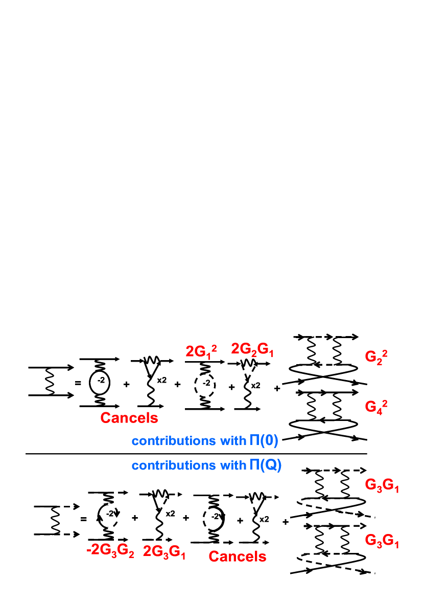
Figure 11: Contributions to the irreducible vertices $\bar{\Gamma}_{hh}^{0}$(top) and $\bar{\Gamma}_{he}$(bottom). $\bar{\Gamma}_{hh}^{0}$ only gets contributions form $\Pi(0)$ while $\bar{\Gamma}_{he}^{0}$ gets contribution from $\Pi(Q)$. From [maiti_rev, ].

The contributions to ${\bar{\Gamma}}^{0}_{hh}$ and ${\bar{\Gamma}}^{0}_{he}$ to order $G^{2}$ are shown in Fig 11. In analytical form I have

$${\bar{\Gamma}}^{0}_{hh} = -G_{4}-\left(G^{2}_{4}+G^{2}_{2}-2G_{1}(G_{1}-G_{2})\right)\Pi_{ph}(0),$$

$${\bar{\Gamma}}^{0}_{he} = -G_{3}-2G_{3}(2G_{1}-G_{2})\Pi_{ph}(Q),$$ (10)

where, I remind, ${\bf Q}=(\pi,\pi)$. For a constant $G$ this reduces to

$${\bar{\Gamma}}^{0}_{hh} = -G\left(1+2G\Pi_{ph}(0)\right),$$

$${\bar{\Gamma}}^{0}_{he} = -G\left(1+2G\Pi_{ph}(Q)\right),$$ (11)

One can show that the relation (LABEL:4_2_1) still holds if we replace $G_{3}$ by $-{\bar{\Gamma}}^{0}_{he}$ and $G_{4}$ by $-{\bar{\Gamma}}^{0}_{hh}$. Because $\Gamma^{full}_{ee}=\Gamma^{full}_{hh}$, I will only deal with $\Gamma^{full}_{hh}$ and $\Gamma^{full}_{he}$, which are given by

$$\Gamma^{full}_{hh} = \frac{1}{2}\left(\frac{{\bar{\Gamma}}^{0}_{he}+{\bar{\Gamma}}^{0}_{hh}}{1-({\bar{\Gamma}}^{0}_{he}+{\bar{\Gamma}}^{0}_{hh})\Pi_{pp}}+\frac{{\bar{\Gamma}}^{0}_{hh}-{\bar{\Gamma}}^{0}_{he}}{1-({\bar{\Gamma}}^{0}_{hh}-{\bar{\Gamma}}^{0}_{he})\Pi_{pp}}\right),$$

$$\Gamma^{full}_{he} = \frac{1}{2}\left(\frac{{\bar{\Gamma}}^{0}_{he}+{\bar{\Gamma}}^{0}_{hh}}{1-({\bar{\Gamma}}^{0}_{he}+{\bar{\Gamma}}^{0}_{hh})\Pi_{pp}}-\frac{{\bar{\Gamma}}^{0}_{hh}-{\bar{\Gamma}}^{0}_{he}}{1-({\bar{\Gamma}}^{0}_{hh}-{\bar{\Gamma}}^{0}_{he})\Pi_{pp}}\right).$$

The condition for the pairing instability becomes $|{\bar{\Gamma}}^{0}_{he}|>-{\bar{\Gamma}}^{0}_{hh}$. Comparing the two irreducible vertex functions, I find

$${\bar{\Gamma}}^{0}_{hh}+|{\bar{\Gamma}}^{0}_{he}|=2G^{2}\left(\Pi_{ph}(Q)-\Pi_{ph}(0)\right)$$ (13)

i.e., the condition for the pairing is satisfied when $\Pi_{ph}(Q)>\Pi_{ph}(0)$. For a gas of fermions with one circular FS, $\Pi_{ph}(q)$ either stays constant or decreases with $q$, and the condition $\Pi_{ph}(Q)>\Pi_{ph}(0)$ cannot be satisfied. However, in our case, the two FS’s are separated by ${\bf Q}$, and, moreover, one FS is of hole type, while the other is of electron type. One can easily verify that, in this situation, $\Pi_{ph}(Q)$ is enhanced comparable to $\Pi_{ph}(0)$. I present the plot of $\Pi_{ph}(q)$ along $q_{x}=q_{y}$ in Fig 12. Indeed, $\Pi_{ph}(Q)$ is much larger than $\Pi_{ph}(0)$.

We see therefore that for the renormalization of the bare interaction into an irreducible pairing vertex does give rise to an attraction in the $A_{1g}$ pairing channel. The attractive pairing interaction is weak and at this stage is certainly smaller than the interaction in the SDW channel. On the other hand, the polarization bubble $\Pi_{ph}(Q)$ is in general some constant, while the polarization bubble $\Pi_{pp}$ diverges logarithmically when the total frequency $\Omega$ vanishes.

Before I proceed, a comment. Because we deal with fermions with circular FSs located near particular $k-$points, polarization operators at small momentum transfer and momentum transfer ${\bf Q}=(\pi,\pi)$ can be approximated by constants. Then the irreducible vertex function has only an $s-$wave ($A_{1g}$) harmonic, like the bare interaction, i.e. KL renormalization does not generate interactions in other channels. Treating pockets as circular is indeed an approximation, because for square lattice the only true requirement is that each FS is symmetric with respect to rotations by multiples of $\pi/2$ ($C_{4}$ symmetry). For small pocket sizes, deviations from circular forms are small, but nevertheless are generally finite. If we include this effect, we find that the KL effect does generate interactions in other channels ($B_{1g},B_{2g}$, and $A_{2g}$), which may be attractive, and also leads to more complex structure of the pair wave function in $s^{+-}$ channel, which now acquires angular dependence along hole and electron pockets, consistent with $C_{4}$ symmetryAccNodes ; Cvetkovic

The Hubbard limit of a constant $G$ is a somewhat artificial case, however. The actual bare interactions $G_{i}$ have to be extracted from the multi-orbital model and do depend on momentum transfer. In this situation $G_{4}-G_{3}$ is generally non-zero already before KL renormalization. It is natural to expect that the bare interaction is a decreasing function of momenta, in which case $G_{4}$, which is the interaction at small momentum transfer, is larger than the interaction $G_{3}$ at momentum transfer near $Q$. Then the KL term has to compete with the first-order repulsion. As long as $G\Pi_{ph}(Q)$ is small, KL renormalization cannot overshoot bare repulsion, and the bound state does not appear. The situation may change when we include momentum dependence of the interaction and non-circular nature of the pockets. In this last case, there appears infinite number of $A_{1g}$ harmonics, which all couple to each other, and in some cases one or several eigenfunctions may end up being attractive A1g ; maiti_11 . Besides, angle dependence generates $d-$wave and $g-$wave harmonics, and some of eigenfunctions in these channels may also become attractive and compete with $s-$wave B1gA1g ; maiti_11 . Still, however, in distinction to the isotropic case, there is no guarantee that “some" eigenfunction from either $A_{1g}$, or $B_{1g}$, or $B_{2g}$, or $A_{2g}$, will be attractive. In other words, a lattice system may well remain in the normal state down to $T=0$.

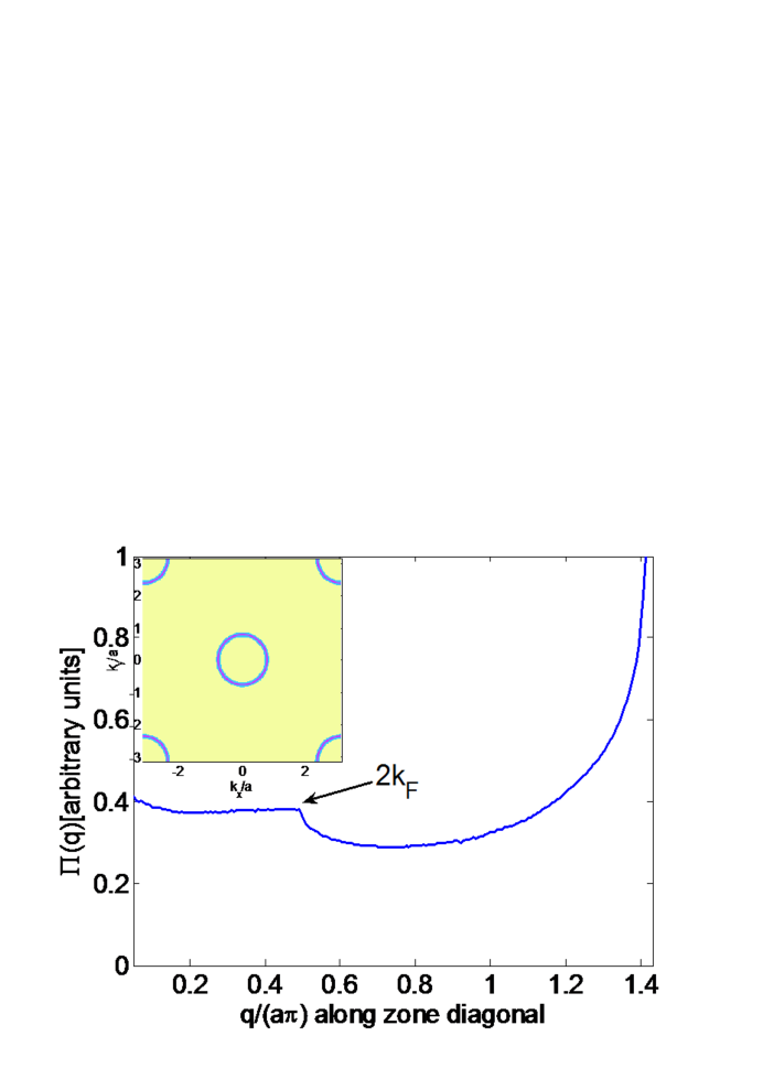
Figure 12: The plot of $\Pi(q)$ for a 2-pocket model with $\vec{q}$ along the zone diagonal. When $\vec{q}<2k_{F}$, $\Pi(q)$ saturates, as it is expected for a 2D system with a circular Fermi surface. Note the $2k_{F}$ cusp-like feature, which is the one-sided $2k_{F}$ non-analyticity of $\Pi(q)$ in 2D. At larger $q$, $\Pi(q)$ gets larger and almost diverges at $\vec{q}\sim\vec{Q}$ due to near-nesting. The inset shows the FS topology for which $\Pi(q)$ has been calculated. The arcs at the corners are parts of the electron pocket and the one in the center is the hole pocket. From [maiti_rev, ; maiti_book, ].

RPA-type approach, spin-mediated interaction

How can we still get superconductivity in this situation? One way to proceed is to apply another ladder summation scheme – this time to series of renormalizations which transform a bare interaction into an irreducible particle-particle vertex. The leading terms in the series are KL terms, but full ladder series include infinite set of higher-order terms. This computational procedure is often called random-phase approximation (RPA) by analogy with the analogous summation scheme to get a screened Coulomb interaction. I skip the details of the calculations (they can be found in, e.g.,  maiti_rev ; scalapino_1 and formally require $\Pi_{ph}(0)\gg\Pi_{ph}(2k_{F})$ and $\Pi_{ph}(Q)\gg\Pi_{ph}(Q+2k_{F})$) and present the result: ladder summation gives rise to an irreducible pairing vertex in the form ${\bar{\Gamma}}^{0}_{\alpha\beta,\gamma\delta}(k,-k;p,-p)=\Gamma_{c}(k-p)\delta_{\alpha\gamma}\delta_{\beta\delta}+\Gamma_{s}(k-p)\vec{\sigma}_{\alpha,\gamma}\cdot\vec{\sigma}_{\beta\delta}$, where for $k$ and $p$ on the same pocket

$$\Gamma_{c}(0)=-\frac{G_{4}}{2}\frac{1}{1+G_{4}\Pi_{ph}(0)}\leavevmode\nobreak\ \leavevmode\nobreak\ \leavevmode\nobreak\ \Gamma_{s}(0)=\frac{G_{4}}{2}\frac{1}{1-G_{4}\Pi_{ph}(0)},$$ (14)

and for $k$ and $p$ at different pockets, when $k-p\approx Q$

$$\Gamma_{c}(Q)=-\frac{G_{3}}{2}\frac{1}{1+G_{3}\Pi_{ph}(Q)}\leavevmode\nobreak\ \leavevmode\nobreak\ \leavevmode\nobreak\ \Gamma_{s}(Q)=\frac{G_{3}}{2}\frac{1}{1-G_{3}\Pi_{ph}(Q)}$$ (15)

Re-expressing ${\bar{\Gamma}}^{0}_{\alpha\beta,\gamma\delta}(k,-k;p,-p)$ in terms of singlet and triplet components as

$${\bar{\Gamma}}^{0}_{\alpha\beta,\gamma\delta}(k,-k;p,-p)=$$

$$\Gamma_{\text{s=0}}(k-p)\left(\delta_{\alpha\gamma}\delta_{\beta\delta}-\delta_{\alpha\delta}\delta_{\beta\gamma}\right)+$$

$$\Gamma_{\text{s=1}}(k-p)\left(\delta_{\alpha\gamma}\delta_{\beta\delta}+\delta_{\alpha\delta}\delta_{\beta\gamma}\right).$$

we obtain

$$\Gamma_{\text{s=0}} = \frac{1}{2}\left(\Gamma_{c}-3\Gamma_{s}\right)$$

$$\Gamma_{\text{s=1}} = \frac{1}{2}\left(\Gamma_{c}+\Gamma_{s}\right)$$ (17)

i.e.

$$\Gamma_{\text{s=0}}(0) = -\frac{G_{4}}{4}\left(\frac{1}{1+G_{4}\Pi_{ph}(0)}+\frac{3}{1-G_{4}\Pi_{ph}(0)}\right)$$

$$\Gamma_{\text{s=1}}(0) = \frac{G_{4}}{4}\left(\frac{1}{1-G_{4}\Pi_{ph}(0)}-\frac{1}{1+G_{4}\Pi_{ph}(0)}\right)$$

$$\Gamma_{\text{s=0}}(Q) = -\frac{G_{3}}{4}\left(\frac{1}{1+G_{3}\Pi_{ph}(Q)}+\frac{3}{1-G_{3}\Pi_{ph}(Q)}\right)$$

$$\Gamma_{\text{s=1}}(Q) = \frac{G_{3}}{4}\left(\frac{1}{1-G_{3}\Pi_{ph}(Q)}-\frac{1}{1+G_{3}\Pi_{ph}(Q)}\right)$$ (18)

Let’s compare this result with what we obtained in the KL formalism. Focus on the singlet channel and expand in (18) to second order in $G_{3,4}$. We have

$$\Gamma_{\text{s=0}}(0)\approx-\frac{G_{4}}{2}\left(1+\frac{1}{1-G_{4}\Pi_{ph}(0)}\right)$$

$$\approx-G_{4}\left(1+0.5G_{4}\Pi_{ph}(0)\right)$$

$$\Gamma_{\text{s=0}}(Q)\approx-\frac{G_{3}}{2}\left(1+\frac{1}{1-G_{3}\Pi_{ph}(Q)}\right)$$

$$\approx-G_{3}\left(1+0.5G_{3}\Pi_{ph}(Q)\right)$$ (19)

Apart from the factor of $1/2$ (which is the consequence of an approximate RPA scheme) $\Gamma_{\text{s=0}}(0)$ is the same as irreducible vertex ${\bar{\Gamma}}^{0}_{11}$, which we obtained in KL calculation in the previous section, and $\Gamma_{\text{s=0}}(Q)$ the same as ${\bar{\Gamma}}^{0}_{12}$ By itself, this is not surprising, as in $\Gamma_{\text{s=0}}$ we included the same particle-hole renormalization of the bare pairing interaction as in the KL formalism.

I now look more closely at the spin-singlet components

$$\Gamma_{\text{s=0}}(0)=-\frac{1}{4}\left(\frac{G_{4}}{1+G_{4}\Pi_{ph}(0)}+\frac{3G_{4}}{1-G_{4}\Pi_{ph}(0)}\right)$$

$$\Gamma_{\text{s=0}}(Q)=-\frac{1}{4}\left(\frac{G_{3}}{1+G_{3}\Pi_{ph}(Q)}+\frac{3G_{3}}{1-G_{4}\Pi_{ph}(Q)}\right),$$ (20)

For repulsive interaction, the charge contribution gets smaller when we add higher terms in $G$ whereas spin contribution gets larger. A conventional recipe in this situation is to neglect all renormalizations in the charge channel and approximate ${\Gamma_{\text{s=0}}}$ with the sum of a constant and the interaction in the spin channel. The irreducible interaction in the $s+-$ channel is then

$$\Gamma_{\text{s=0}}(0)-\Gamma_{\text{s=0}}(Q)=$$

$$\frac{-G_{4}+G_{3}}{4}-\frac{3}{4}\left(\frac{G_{4}}{1-G_{4}\Pi_{ph}(0)}-\frac{G_{3}}{1-G_{3}\Pi_{ph}(Q)}\right)$$

Like I said before, if $G_{4}\Pi_{ph}(0)$ and $G_{3}\Pi_{ph}(Q)$ are both small, $G_{4}-G_{3}$ term is the largest and the pairing interaction is repulsive for $G_{4}>G_{3}$. However, we see that there is a way to overcome the initial repulsion: if $G_{3}\Pi_{ph}(Q)>G_{4}\Pi_{ph}(0)$, one can imagine a situation when $G_{3}\Pi_{ph}(Q)\approx 1$, and the correction term in (III.2.1) becomes large and positive and can overcome the negative first-order term.

What does it mean from physics perspective? We found earlier that the condition $G_{3}\Pi_{ph}(Q)=1$ signals an instability of a metal towards a SDW order with momentum Q. We don’t need the order to develop, but we need SDW fluctuations to be strong and to mediate pairing interaction between fermions. Once spin-mediated interaction exceeds bare repulsion, the irreducible pairing interaction in the corresponding channel becomes attractive. Notice in this regard that we need magnetic fluctuations to be peaked at large momentum transfer $Q$. If they are peaked at small momenta, $\Pi_{ph}(0)$ exceeds $\Pi_{ph}(Q)$, and the interaction in the singlet channel remains repulsive.

Spin-fluctuation approach

What I just described is the main idea of the spin-fluctuation-mechanism of superconductivity. The effective pairing interaction can be obtained either within RPApeter ; Kuroki_2 or, using one of several advanced numerical methods developed over the last decade, or just introduced semi-phenomenologically. The semi-phenomenological model is called the spin-fermion modelacs . Quite often, interaction mediated by spin fluctuations also critically affects single-fermion propagator (the Green’s function), and this renormalization has to be included into the pairing problem. As another complication, the interaction mediated by soft spin fluctuations has a strong dynamical part due to Landau damping – the decay of a spin fluctuation into a particle-hole pair. This dynamics also has to be included into consideration, which makes the solution of the pairing problem near a magnetic instability quite involved theoretical problem.

There are two crucial aspects of the spin-fluctuation approach acs ; maiti_book . First, magnetic fluctuations have to develop at energies much larger than the ones relevant for the pairing, typically at energies comparable to the bandwidth $W$. It is crucial for spin-fluctuation approach that SDW magnetism is the only instability which develops at such high energies. There may be other instabilities (e.g., charge order), but the assumption is that they develop at small enough energies and can be captured within the low-energy model with spin fluctuations already presentEfetov3 ; Senthil ; wang . Second, spin-fluctuation approach is fundamentally not a weak coupling approach. In the absence of nesting, $\Pi_{ph}(Q)$ and $\Pi_{ph}(0)$ are generally of order $1/W$, and $\Pi_{ph}(Q)$ is only larger numerically. Then the interaction $G_{3}$ must be of order $W$ in order to get a strong magnetically-mediated component of the pairing interaction,

One way to proceed in this situation is to introduce the spin-fermion model with static magnetic fluctuations built into it, and then assume that within this model the interaction between low-energy fermions ${\bar{g}}$ is smaller than $W$ and do controlled low-energy analysis treating $\bar{g}/W$ as a small parameteracs ; Efetov3 ; Senthil . There are several ways to make the assumptions ${\bar{g}}\ll W$ and $G\sim W$ consistent with each other, e.g., if microscopic interaction has length $\Gamma_{0}$ and $\Gamma_{0}k_{F}/\hbar\gg 1$, then ${\bar{g}}$ is small in $1/(\frac{\Gamma_{0}k_{F}}{\hbar})$ compared to $G$ (Refs.cm ; Dzero ). At the same time, the properties of the spin-fermion model do not seem to crucially depend on ${\bar{g}}/W$ ratio, so the hope is that, even if the actual ${\bar{g}}$ is of order $W$, the analysis based on expansion in ${\bar{g}}/W$ captures the essential physics of the pairing system behavior near a SDW instability in a metal.

IV Interplay between SDW magnetism and superconductivity, parquet RG approach

I now return to weak coupling, where I have control over calculations, and ask the question whether one can still get an attraction in at least one pairing channel despite that $G_{4}>G_{3}$, i.e., the bare pairing interaction is repulsive in all channels. The answer is, actually, yes, it is possible, but under a special condition that $\Pi_{ph}(Q)$ is singular and diverges logarithmically at zero frequency or zero temperature, in the same way as the particle-particle bubble $\Pi_{pp}(0)$. This condition is satisfied exactly when there is a perfect nesting between fermionic excitations separated by $Q$. For Fe-pnictides, it implies that hole and electron FSs perfectly match each other when one is shifted by $Q$.

I show below that $\Pi_{ph}(Q)$ and $\Pi_{pp}(0)$ do have exactly the same logarithmic singularity at perfect nesting. At the moment, let’s take this for granted and compare the relevant scales. First, no fluctuations develop at energies/temperatures of order $W$ because at such high scales the logarithmical behavior of $\Pi_{pp}$ and $\Pi_{ph}$ is not yet developed and both bubbles scale as $1/W$. At weak coupling $G/W<<1$, hence corrections to bare vertices are small at these energies. Second, we know that the pairing vertex evolves at $(G_{3}-G_{4})\Pi_{pp}(0)\sim O(1)$, and that corrections to the bare irreducible pairing vertex become of order one when $G_{3}\Pi_{ph}(Q)\sim O(1)$. But we also know from, e.g., (15) that at the same scale the SDW vertex begins to evolve. Moreover other inter-pocket interactions, which we didn’t include so far: density-density and exchange interactions (which here and below we label as $G_{1}$ and $G_{2}$, respectively) also start evolving because their renormalization involves terms $G_{1}\Pi_{ph}(Q)$ and $G_{2}\Pi_{ph}(Q)$, which also become of $O(1)$, provided that all bare interactions are of the same order. Once $G_{1,2}\Pi_{ph}(Q)$ becomes of order one, the renormalization of $G_{3}$ by $G_{1}$ and $G_{2}$ interactions also becomes relevant. The bottom line here is that renormalization of all interactions become relevant at the same scale where $G_{i}\Pi_{ph}(Q)\sim G_{i}\Pi_{pp}(0)\sim 1$. At this scale we can expect superconductivity, if the corrections to $G_{4}-G_{3}$ overcome the sign of the pairing interaction, and we also we can expect an instability towards SDW and, possibly, towards some other order. The issue then is whether it is possible to construct a rigorous description of the system behavior in the situation when all couplings are small compared to $W$, but $G_{i}\Pi_{ph}(Q)$ and $G_{i}\Pi_{pp}(0)$ are of order one. The answer is yes, and the corresponding procedure is called a parquet renormalization group (pRG).

The pRG is a controlled weak coupling approach. It assumes that no correlations develop at energies comparable to the bandwidth, but that there are several competing orders whose fluctuations develop simultaneously at smaller energies. Superconductivity is one of them, others include SDW and potential charge-density-wave (CDW), nematic and other orders. The pRG approach treats superconductivity, SDW, CDW and other potential instabilities on equal footings. Correlations in each channel grow up with similar speed, and fluctuations in one channel affect the fluctuations in the other channel and vise versa. For superconductivity, once the corrections to the pairing vertex become of order one, and there is a potential to convert initial repulsion into an attraction. We know that second-order contribution to the pairing vertex from SDW channel works in the right direction, and one may expect that higher-order corrections continue pushing the pairing interaction towards an attraction. However even if attraction develops, there is no guarantee that the system will actually undergo a SC transition because it is entire possible that SDW instability comes before SC instability.

The pRG approach addresses both of these issues. It can be also applied to a more realistic case of non-perfect nesting if deviations from nesting are small in the sense that there exists a wide range of energies where $\Pi_{ph}(Q)$ and $\Pi_{pp}(0)$ are approximately equal. Below some energy scale, $\omega_{0}$, the logarithmical singularity in $\Pi_{ph}(Q)$ is cut. If this scale is smaller than the one at which the leading instability occurs, a deviation from a perfect nesting is an irrelevant perturbation. If it is larger, then pRG runs up to $\omega_{0}$, and at smaller energies only SC channel continues to evolve in BCS fashion.

There also exists a well-developed numerical computational procedure called functional RG (fRG)frg1 ; frg2 ; dhl . Its advantage is that it is not restricted to a small number of patches and captures the evolution of the interactions in various channels even if the interactions depend on the angles along the FS. The “price" one has to pay is the reduction in the control over calculations – fRG includes both leading and subleading logarithmical terms. If only logarithmical terms are left, the angle dependencies of the interactions do not evolve in the process of RG flow, only the overall magnitude changesRG_SM So far, the results of fRG and pRG analysis for various systems fully agree. Below I focus on the pRG approach. For the thorough tutorial on the RG technique, see Ref. shankar . In the discussion below and in Sec. 8.5 I follow Refs. [maiti_rev, ; maiti_book, ].

IV.1 Parquet Renormalization Group: The Basics

I recall that in Fe-pnictides a bubble with momentum transfer $Q$ contains one hole (c) and one electron (f) propagator, and at perfect nesting the dispersions of holes and electrons are just opposite, $\varepsilon_{c}(k)=-\varepsilon_{f}(k+Q)$. The particle-hole and particle-particle bubbles are

$$\Pi_{pp}(0) = -i\int\frac{d^{2}k\;d\omega}{(2\pi\hbar)^{3}}G^{c}(k,\omega)G^{c}(-k,-\omega)$$

$$\Pi_{ph}(Q) = i\int\frac{d^{2}k\;d\omega}{(2\pi\hbar)^{3}}G^{c}(k,\omega)G^{f}(Q+k,\omega),$$ (22)

where

$G^{c,f}=\frac{1}{\omega-\varepsilon^{c,f}_{k}+i\delta sgn(\omega)}$. Substituting into Eq. IV.1 and using $\varepsilon_{c}(k)=-\varepsilon_{f}(k+Q)$ one can easily make sure that the two expressions in Eq. IV.1 are identical. Evaluating the integrals we obtain

$$\Pi_{pp}(0)=\Pi_{ph}(Q)=N_{0}L+...$$ (23)

where $N_{0}=m/2\pi\hbar^{2}$ is the 2D density of states,

$$L=\frac{1}{2}\log\left(\frac{W}{E}\right),$$ (24)

$E$ is a typical energy of an external fermion, and the dots stand for non-logarithmic terms. The factor $1/2$ is specific to the pocket model and accounts for the fact that for small pocket sizes, the logarithm comes from integration over positive energies $W>E>E_{F}$. At non-perfect nesting, the particle-particle channel is still logarithmic, but the particle-hole channel gets cut by the energy difference ($\delta E$) associated with the nesting mismatch, such that

$$\Pi_{ph}(Q)=N_{0}\log\frac{W}{\sqrt{E^{2}+\delta E^{2}}}$$ (25)

The main idea of pRG (as of any RG procedure) is to consider $E$ as a running variable, assume that initial $E$ is comparable to $W$ and $G_{i}\log\left(\frac{W}{E}\right)=G_{i}L$ is small, calculate the renormalizations of all couplings by fermions with energies larger than $E$, and find how the couplings evolve as $E$ approaches the region where $G_{i}L=O(1)$.

This procedure can be carried out already in BCS theory, because Cooper renormalizations are logarithmical. For an isotropic system, the evolution of the interaction $U_{l}$ in a channel with angular momentum $l$ due to Cooper renormalization can be expressed in RG treatment as an equation for the running coupling $U_{l}(L)$

$$\frac{dU_{l}(L)}{dL}=-N_{0}\left(U_{l}(L)\right)^{2}.$$ (26)

The solution of (26) is

$$U_{l}(L)=\frac{U_{l}}{1+U_{l}N_{0}L}.$$ (27)

Similar formulas can be obtained in lattice systems when there are no competing instabilities, i.e., only renormalizations in the pairing channel are relevant. For example, in the two-pocket model for the pnictides, the equations for the vertices $\Gamma_{hh}(L)=-G_{4}(L)$ and $\Gamma_{he}(L)=-G_{3}(L)$, Eqs. (LABEL:4_2_1), can be reproduced by solving the two coupled RG equations

$$\frac{dG_{3}(L)}{dL}=-2N_{0}G_{3}(L)G_{4}(L)$$

$$\frac{dG_{4}(L)}{dL}=-N_{0}\left(\left(G_{3}(L)\right)^{2}+\left(G_{4}(L)\right)^{2}\right)$$ (28)

with boundary conditions $G_{4}(L=0)=G_{4}$, $G_{3}(L=0)=G_{3}$. The set can be factorized by introducing $G_{A}(L)=G_{3}(L)+G_{4}(L)$ and $G_{B}(L)=G_{4}(L)-G_{3}(L)$ to

$$\frac{dG_{A}(L)}{dL}=-N_{0}\left(G_{A}(L)\right)^{2},\leavevmode\nobreak\ \leavevmode\nobreak\ \frac{dG_{B}(L)}{dL}=-N_{0}\left(G_{B}(L)\right)^{2}$$ (29)

The solution of the set yields

$$G_{A}(L)=G_{4}(L)+G_{3}(L)=\frac{G_{3}+G_{4}}{1+N_{0}L(G_{3}+G_{4})}$$

$$G_{B}(L)=G_{4}(L)-G_{3}(L)=\frac{G_{4}-G_{3}}{1+N_{0}L(G_{4}-G_{3})}$$ (30)

Solving this set and using $\Gamma_{hh}(L)=-G_{4}(L)$, $\Gamma_{he}(L)=-G_{3}(L)$, we reproduce (LABEL:4_2_1). This returns us to the same issue as we had before, namely if $G_{4}>G_{3}$, the fully renormalized pairing interaction does not diverge at any $L$ and in fact decays as $L$ increases: $G_{4}(L)$ decays as $1/L$ and $G_{3}(L)$ decays even faster, as $1/L^{2}$.

I now consider how things change when $\Pi_{ph}(Q)$ is also logarithmical and the renormalizations in the particle-hole channel have to be included on equal footings with renormalizations in the particle-particle channel.

IV.2 pRG in a 2-pocket model

Because two types of renormalizations are relevant, we need to include into consideration all vertices with either small total momentum or with momentum transfer near $Q$ i.e., use the full low-energy Hamiltonian of Eq. (III). There are couplings $G_{3}$ and $G_{4}$ which are directly relevant for superconductivity, and also the couplings $G_{1}$ and $G_{2}$ for density-density and exchange interaction between hole and electron pockets, respectively. These are shown in Fig. 8.

The strategy to obtain one-loop pRG equations, suitable to our case, is the following: One has to start with perturbation theory and obtain the variation of each full vertex $\delta G_{i}$ to order $G_{i}G_{j}L$. Then one has to replace $\delta G_{i}/L$ by $dG_{i}(L)/dL$ and also replace $G_{i}G_{j}$ in the r.h.s. by $G_{i}(L)G_{j}(L)$. The result is the set of coupled differential equations for $dG_{i}(L)/dL$ whose right sides are given by bilinear combinations of $G_{i}(L)G_{j}(L)$. The procedure may look a bit formal, but one can rigorously prove that it is equivalent to summing up series of corrections to $G_{i}$ in powers of $G_{i}L$, neglecting corrections terms with higher powers of $G_{i}$ than of $L$. One can go further and collecting correction terms of order $G_{i}G_{j}G_{k}L$. This is called 2-loop order, and 2-loop terms give contributions of order $(G(L))^{3}$ to the right side of the equations for $dG_{i}(L)/dL$. 2-loop calculations are, however, quite involvedbrazil and have not been re-checked. Below I only consider 1-loop pRG equations.

$\begin{array}[]{cc}\includegraphics[width=195.12767pt]{g_1g_2}&\leavevmode\nobreak\ \leavevmode\nobreak\ \leavevmode\nobreak\ \leavevmode\nobreak\ \leavevmode\nobreak\ \leavevmode\nobreak\ \includegraphics[width=195.12767pt]{g_3g_4}\end{array}$

Figure 13: The pRG diagrams to one loop order, which contribute to the parquet flow of $g_{1}$, $g_{2}$, $g_{3}$ and $g_{4}$ vertices. From [maiti_rev, ; maiti_book, ].

The $G^{2}$ corrections to all four couplings are shown in Fig.13. Evaluating the integrals and following the recipe we obtain

$$\dot{g}_{1}=g_{1}^{2}+g_{3}^{2}$$

$$\dot{g}_{2}=2g_{2}(g_{1}-g_{2})$$

$$\dot{g}_{3}=2g_{3}(2g_{1}-g_{2}-g_{4})$$

$$\dot{g}_{4}=-g_{3}^{2}-g_{4}^{2}$$

where we introduced $g_{i}\equiv g_{i}(L)=G_{i}(L)N_{0}$ and $\dot{g}_{i}=dg_{i}/dL$

We note that the renormalizations of $g_{4}$ are still only in the Cooper channel and causes $g_{4}$ to reduce. But for $g_{3}$ we now have a counter-term from $g_{1}$, which pushes $g_{3}$ up. And the $g_{1}$ term is in turn pushed up by $g_{3}$. Thus already at this stage one can qualitatively expect $g_{3}$ to eventually get larger. Fig 14 shows the solution of (IV.2)– the flow of the four couplings for this model. We see that, even if $g_{3}$ is initially smaller than $g_{4}$, it flows up with increasing $L$, while $g_{4}$ flows to smaller values. At some $L=L_{0}$, $g_{3}$ crosses $g_{4}$, and at larger $L$ the pairing interaction $g_{4}-g_{3}$ becomes negative (i.e., attractive). In other words, in the process of pRG flow, the system self-generates attractive pairing interaction. I remind that the attraction appears in the $s^{+-}$ channel. The pairing interaction in $s^{++}$ channel: $g_{3}+g_{4}$ remains positive (repulsive) despite that $g_{4}$ eventually changes sign and becomes negative. It is essential that for $L\sim L_{0}$ the renormalized $g_{i}$ are still of the same order as bare couplings, i.e., are still small, and the calculations are fully under control. In other words, the sign change of the pairing interaction is a solid result, and higher-loop corrections may only slightly shift the value of $L_{0}$ when it happens.

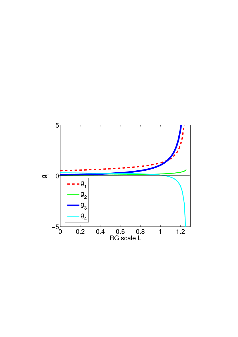
Figure 14: The flow of dimensionless couplings $g_{1,2,3,4}$. $g_{3}$ grows and eventually crosses $g_{4}$, which becomes negative at a large enough RG scale. From [cee, ].

At some larger $L=L_{c}$, the couplings diverge, signaling the instability towards an ordered state (which one I discuss later). One-loop pRG is valid "almost" all the way to the instability, up to $L_{c}-L\sim O(1)$, when the renormalized $g_{i}$ become of order one. At smaller distances from $L_{c}$ higher-loop corrections become relevant. It is very unlikely, however, that these corrections will change the physics in any significant way.

The sign change of the pairing interaction can be detected also if the nesting is not perfect and $\Pi_{ph}(Q)$ does not behave exactly in the same way as $\Pi_{pp}(0)$. The full treatment of this case is quite involved. For illustrative purposes I follow the approach first proposed in Ref.Furukawa and measure the non-equivalence between $\Pi_{pp}(0)$ and $\Pi_{ph}(Q)$ by introducing a phenomenological parameter $d_{1}=\Pi_{ph}(Q)/\Pi_{pp}(0)$ and treat $d_{1}$ as an $L-$ independent constant $0<d_{1}<1$, independent on $L$. This is indeed an approximation, but it is at least partly justified by our earlier observation that the most relevant effect for the pairing is the sign change of $g_{4}-g_{3}$ at some scale $L_{0}$, and around this scale $d_{1}$ is not expected to have strong dependence on $L$. The case $d_{1}=1$ corresponds to perfect nesting, and the case $d_{1}=0$ implies that particle-hole channel is irrelevant, in which case, I remind, $g_{4}-g_{3}$ remains positive for all $L$.

The pRG equations for arbitrary $d_{1}$ are straightforwardly obtained using the same strategy as in the derivation of (IV.2), and the result is cee ; rahul ; podolsky

$$\dot{g}_{1}=d_{1}(g_{1}^{2}+g_{3}^{2})$$

$$\dot{g}_{2}=2d_{1}g_{2}(g_{1}-g_{2})$$

$$\dot{g}_{3}=2d_{1}g_{3}(2g_{1}-g_{2})-2g_{3}g_{4}$$

$$\dot{g}_{4}=-g^{2}_{3}-g^{2}_{4}$$

In Fig 15 I show the behavior of the couplings for representative $0<d_{1}<1$. Like before, I take bare value of $g_{4}$ to be larger than the bare $g_{3}$, i.e., at high energies the pairing interaction is repulsive. This figure and analytical consideration shows that for any non-zero $d_{1}$ the behavior is qualitatively the same as for perfect nesting, i.e., at some $L_{0}<L_{c}$ the running couplings $g_{3}$ and $g_{4}$ cross, and for larger $L$ (smaller energies) pairing interaction in $s^{+-}$ channel becomes attractive. The only effect of making $d_{1}$ smaller is the increase in the value of $L_{0}$. Still, for sufficiently small bare couplings, the range where the pairing interaction changes sign is fully under control in one-loop pRG theory.

$\begin{array}[]{ccc}\includegraphics[width=166.2212pt]{flow_d1}&\includegraphics[width=166.2212pt]{flow_dp3}&\includegraphics[width=166.2212pt]{flow_dp05}\end{array}$

Figure 15: The flow of ratio of couplings $g_{3}/g_{1}$ and $g_{4}/g_{1}$ for different nesting parameters $d_{1}=1$(a), $d_{1}=0.3$(b),$d_{1}=0.05$(c). All cases are qualitatively similar in that $g_{3}/g_{1}$ eventually crosses $g_{4}/g_{1}$. The smaller is the nesting parameter, the ‘later’ is this crossing. If $d_{1}=0$, this crossing will never happen and $g_{4}>g_{3}$ for all $L$.

A way to see analytically that $g_{3}-g_{4}$ changes sign and becomes positive is to consider the system behavior near $L=L_{c}$ and make sure that in this region $g_{3}>g_{4}$. One can easily make sure that all couplings diverge at $L_{c}$, and their ratios tend to some constant values (see discussion around Eq. (V.1) below for more detail). Introducing $g_{2}=ag_{1},g_{3}=bg_{1}$, and $g_{4}=cg_{1}$, and substituting into (IV.2) we find an algebraic set of equations for $a,b$, and $c$. Solving the set, we find that $b=\frac{\sqrt{\sqrt{16d_{1}^{4}-4d_{1}^{2}+4}+2-d_{1}^{2}}}{d_{1}}$and $c=\frac{d_{1}}{2}(3-b^{2})$. The negative sign of $c$ and positive sign of $b$, combined with the fact that $g_{1}$ definitely increases under the flow and surely remains positive, imply that near $L_{c}$, $g_{4}$ is negative, while $g_{3}$ is positive (this is also evident from the Fig 15). Obviously then, $g_{3}$ and $g_{4}$ must cross at some $L_{0}<L_{c}$.

The reason for the sign change of the pairing interaction is clear from the structure of the pRG equation for $g_{3}$ the r.h.s. of which contains the term $4d_{1}g_{3}g_{4}$, which pushes $g_{3}$ up. We know from second-order KL calculation that the upward renormalization of $g_{3}$ comes from the magnetic channel and can be roughly viewed as the contribution from spin-mediated part of effective fermion-fermion interaction. Not surprisingly, we will see below that $g_{1}$ does, indeed, contribute to the SDW vertex. From this perspective, the physics of the attraction in pRG (or in fRG, which brings in the same conclusions as pRG) and in spin-fermion model is the same: magnetic fluctuations push inter-pocket/inter-patch interaction up, and below some energy scale the renormalized inter-pocket/inter-patch interaction becomes larger than repulsive intra-pocket/intra-patch interaction.

There is, however, one important difference between the RG description and the description in terms of spin-fermion model. In the spin-fermion model, magnetic fluctuations are strong, but the system is assumed to be at some distance away from an SDW instability. In this situation, SC instability definitely comes ahead of SDW magnetism. There may be other instabilities produced by strong spin fluctuations, like CDWMax ; efetov ; Physics ; wang ; sachdev_new ; pdw , which compete with SC and, by construction, also occur before SDW order sets in.

In RG treatment (pRG or fRG), SDW magnetism and SC instability (and other potential instabilities) compete with each other, and which one develops first needs to be analyzed. So far, we only found that SC vertex changes sign and becomes attractive. But we do not know whether superconductivity is the leading instability, or some other instability comes first. This is what we will study next. The key issue, indeed, is whether superconductivity can come ahead of SDW magnetism, whose fluctuations helped convert repulsion in the pairing channel into an attraction.

V Competition between density wave orders and superconductivity

Thus far, we identified an instability in a particular channel with the appearance of a pole in the upper frequency half-plane in the corresponding vertex – the vertex with zero total momentum in the case of SC instability, and the vertex with the total momentum $Q$ in the case of SDW instability. Since our goal is to address the competition between these states, it is actually advantageous to use a slightly different approach: introduce all potentially relevant fluctuating fields, use them to decouple 4-fermion terms into a set of terms containing two fermions and a fluctuating field, compute the renormalization of these “three-legged" vertices and use these renormalized vertices to obtain the susceptibilities in various channels and check which one is the strongest. We will see that the renormalized vertices in different channels (most notably, SDW and SC) do diverge near $L_{c}$, but with different exponents. The leading instability will be in the channel for which the exponent is the largest. There is one caveat in this approach — for a divergence of the susceptibility the exponent for the vertex should be larger than $1/2$ (Ref.Cvetkovic ), but we will see below that this condition is satisfied, at least for the leading instability.

V.1 Two pocket model

Let us see how it works for a two-pocket model. There are two particle-particle three legged vertices $\Gamma_{h,e}$ as shown in Fig 16. To obtain the flow of these vertices, i.e., $\Gamma^{SC}_{h,e}(L)$ I assume that external fermions and a fluctuating field have energies comparable to some E (i.e.,$L=\log\Lambda/E$) and collect contributions from all fermions with energies larger than $E$. To do this with logarithmical accuracy I write all possible diagrams, choose a particle-particle cross-section at the smallest internal energy $E^{\prime}\geq E$ and sum up all contributions to the left and to the right of this cross-section, as shown in Fig 17. The sum of all contributions to the left of the cross-section gives the three legged vertex at energy $E^{\prime}$ (or $L^{\prime}=\log\Lambda/E^{\prime}$), and the sum of all contributions to the right of the cross-section gives the interaction $g_{i}$ at energy $L^{\prime}$. The integration over the remaining cross-section gives $\int^{L}dL^{\prime}$ (with our normalization of $g_{i}$), and the equation for, e.g., $\Gamma_{h}(L)$ becomes

$$\Gamma^{SC}_{h}(L)=\int^{L}dL^{\prime}\left(\Gamma^{SC}_{h}(L^{\prime})g_{4}(L^{\prime})+\Gamma^{SC}_{e}(L^{\prime})g_{3}(L^{\prime})\right)$$ (33)

Differentiating over the upper limit, we obtain differential equation for $d\Gamma^{SC}_{h}(L)/dL$ whose r.h.s. contains $\Gamma^{SC}_{h,e}(L)$ and $g_{3,4}(L)$ at the same scale $L$.

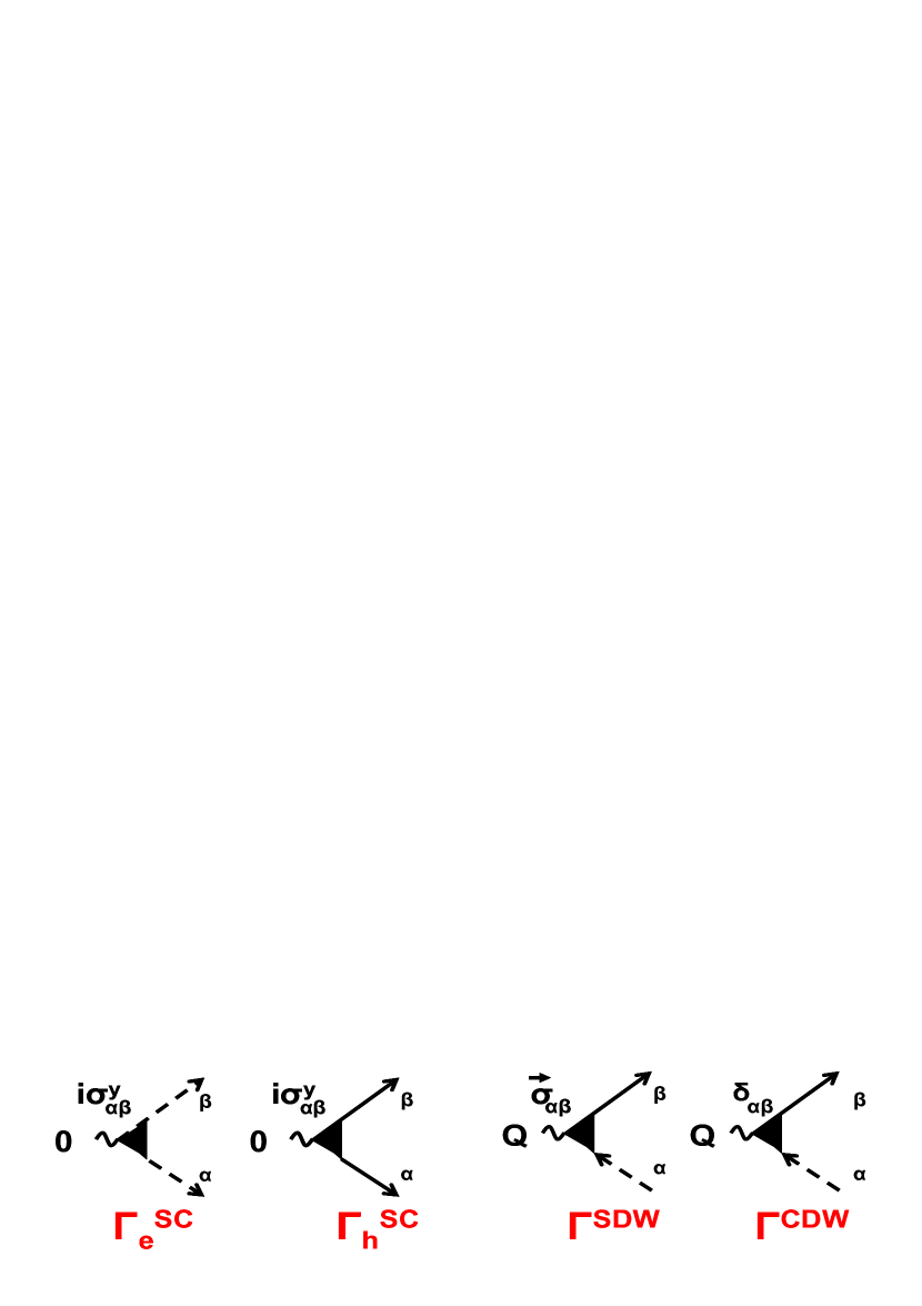
Figure 16: Superconducting and density-wave three-leg vertices. Divergence of any of these vertices indicates that the system is likely to be unstable to the corresponding order. $\Gamma^{SC}_{h,e}$ are superconducting vertices, $\Gamma^{SDW}$ is SDW vertex and $\Gamma^{CDW}$ is CDW vertex. From [cee, ].

Figure 17: The flow diagrams for the effective vertices: SC vertex (top two) and SDW vertex (bottom). The couplings $g_{i}$’s here are running couplings in RG sense. From [maiti_rev, ; maiti_book, ].

Collecting the contributions for $\Gamma^{SC}_{h}(L)$ an $\Gamma^{SC}_{e}(L)$ we obtain

$$\frac{d\Gamma^{SC}_{h}}{dL} = \Gamma^{SC}_{h}g_{4}+\Gamma^{SC}_{e}g_{3}$$

$$\frac{d\Gamma^{SC}_{e}}{dL} = \Gamma^{SC}_{e}g_{4}+\Gamma^{SC}_{h}g_{3}$$

or

$$\frac{d\Gamma_{++}}{dL} = (g_{4}+g_{3})\Gamma_{++}$$

$$\frac{d\Gamma_{+-}}{dL} = (g_{4}-g_{3})\Gamma_{+-}$$

where $\Gamma_{++}\equiv\Gamma^{SC}_{h}+\Gamma^{SC}_{e}$ and $\Gamma_{+-}\equiv\Gamma^{SC}_{h}-\Gamma^{SC}_{e}$. The first one is for $s^{++}$ pairing, the second is for $s^{+-}$ pairing. We have seen in the previous section that the running couplings $g_{3,4}$ diverge at some critical RG scale $L_{c}$. The flow equation near $L_{c}$ is in the form $\dot{g}\sim g^{2}$, hence

$$g_{i}=\frac{\alpha_{i}}{L_{c}-L}.$$ (36)

Substituting this into Eq. V.1 and solving the differential equation for $\Gamma$ we find that the two SC three legged vertices behave as

$$\Gamma_{s^{++}}\propto\frac{1}{(L_{c}-L)^{-\alpha_{3}-\alpha_{4}}},\leavevmode\nobreak\ \leavevmode\nobreak\ \Gamma_{s^{+-}}=\frac{1}{(L_{c}-L)^{\alpha_{3}-\alpha_{4}}},$$ (37)

The requirement for the divergence of $\Gamma_{s^{+-}}$ is $\alpha_{3}>\alpha_{4}$, which is obviously the same as $g_{3}>g_{4}$ (see (36)).

I follow the same procedure for an SDW vertex ${\vec{\Gamma}}^{SDW}_{\alpha\beta}=\Gamma^{SDW}{\vec{\sigma}}_{\alpha\beta}$. I introduce a particle-hole vertex with momentum transfer $Q$ and spin factor ${\vec{\sigma}}_{\alpha\beta}$, as shown in Fig 16, and obtain the equation for $d\Gamma^{SDW}(L)/dL$ in the same way as we did for SC vertices. We obtain (see Fig. 17)

$$\frac{d\Gamma^{SDW}}{dL} = d_{1}(g_{1}+g_{3})\Gamma^{SDW}$$

Using Eq. 36 and following the same steps as above we obtain at $L\approx L_{c}$

$$\Gamma^{SDW}\propto\frac{1}{(L_{c}-L)^{d_{1}(\alpha_{1}+\alpha_{3})}}$$ (39)

For CDW vertex (the one with the overall factor $\delta_{\alpha\beta}$ instead ${\vec{\sigma}}_{\alpha\beta}$), the flow equation is

$$\frac{d\Gamma^{CDW}}{dL} = d_{1}(g_{1}+g_{3}-2g_{3}-2g_{2})\Gamma^{CDW}$$ (40)

$$= d_{1}(g_{1}-g_{3}-2g_{2})\Gamma^{CDW}$$

Using the same procedure as before we obtain

$$\Gamma^{CDW}=\frac{1}{(L_{c}-L)^{d_{1}(\alpha_{1}-\alpha_{3}-2\alpha_{2})}}$$ (41)

The exponents $\alpha_{i}$ can be easily found by plugging in the asymptotic forms in Eq. 36 into the RG equations. This gives the following set of non linear algebraic equations in $\alpha_{i}$

$$\alpha_{1} = d_{1}(\alpha_{1}^{2}+\alpha_{3}^{2})$$

$$\alpha_{2} = 2d_{1}\alpha_{2}(\alpha_{1}-\alpha_{2})$$

$$\alpha_{3} = 2d_{1}\alpha_{3}(2\alpha_{1}-\alpha_{2})-2\alpha_{3}\alpha_{4}$$

$$\alpha_{4} = -\alpha_{3}^{2}-\alpha_{4}^{2}$$

Consider first the case of perfect nesting, $d_{1}=1$. The solution of the set of equations is $\alpha_{1}=\frac{1}{6}$, $\alpha_{2}=0$, $\alpha_{3}=\frac{\sqrt{5}}{6}$ and $\alpha_{4}=-\frac{1}{6}$; Combining $\alpha$’s, we find that the exponents for superconducting and spin density wave instabilities and positive and equal:

$$\alpha_{s\pm} \equiv \alpha_{3}-\alpha_{4}=\frac{1+\sqrt{5}}{6}\approx 0.539$$

$$\alpha_{SDW} \equiv \alpha_{1}+\alpha_{3}=\frac{1+\sqrt{5}}{6}\approx 0.539$$

while the exponent for CDW and $s++$ vertices are negative

$$\alpha_{CDW} = \alpha_{1}+\alpha_{3}=\frac{1-\sqrt{5}}{6}\approx-0.206$$

$$\alpha_{s++} = -\alpha_{3}-\alpha_{4}=\frac{1-\sqrt{5}}{6}\approx-0.206$$ (44)

We see that the superconducting ($s^{+-}$) and SDW channels have equal susceptibilities in this approximation, while CDW channel is not a competitor.

The analysis can be extended to $d_{1}<1$. I define $\beta\equiv\alpha_{4}/\alpha_{1}$, $\gamma\equiv\alpha_{3}/\alpha_{1}$ and obtain

$$\gamma^{2} = \frac{\sqrt{16d_{1}^{4}-4d_{1}^{2}+4}+2-d_{1}^{2}}{d_{1}^{2}}$$

$$\beta = \frac{d_{1}}{2}\left(3-\gamma^{2}\right)$$

$$\alpha_{1} = \frac{1}{d_{1}}\frac{1}{1+\gamma^{2}}$$ (45)

In Fig18 I plot $\alpha_{s\pm}=\alpha_{3}-\alpha_{4}$, $\alpha_{SDW}=\alpha_{1}+\alpha_{3}$, and $\alpha_{CDW}=\alpha_{1}-\alpha_{3}$, We clearly see that (i) CDW channel is never a competitor, and (ii) as $d_{1}$ decreases (the nesting gets worse), the pairing vertex diverges with a higher exponent that SDW channel, hence $s^{+-}$ superconductivity becomes the leading instability, overshooting the channel which helped SC vertex to change sign in the first place.

In real systems, pRG equations are only valid up to some distance from the instability at $L_{c}$. Very near $L_{c}$ three-dimensional effects, corrections from higher-loop orders and other perturbations likely affect the flow of the couplings. Besides, in pocket models, the pRG equations are only valid for $E$ between the bandwidth $W$ and the Fermi energy $E_{F}$. At $E<E_{F}$, internal momenta in the diagrams, which account for the flow of the couplings, become smaller than external $k_{F}$, and the renormalization of $g_{i}$ start depending on the interplay between all four external momenta in the verticesrev_physica ; RG_SM . The calculation of the flow in this case is technically more involved, but the result is physically transparent – SDW and $s^{+-}$ SC channels stop talking to each other, and the vertex evolves according to Eqs. (37) and (V.1), with $g_{i}$ taken at the scale $E_{F}$ (or $L_{F}=\log\Lambda/E_{F}$). If $L_{F}>L_{c}$, the presence of the scale set by the Fermi energy is irrelevant, but if $L_{F}<L_{c}$ (which is the case for the Fe-pnictides because superconducting $T_{c}$ and magnetic $T_{SDW}$ are much smaller than $E_{F}$), then one should stop pRG flow at $L_{E_{F}}$. At perfect nesting, the SDW combination $g_{1}+g_{3}$ is larger than $s^{+-}$ combination $g_{3}-g_{4}$ at any $L<L_{c}$, hence SDW channel wins, and the leading instability upon cooling down the system is towards a SDW order. At non-zero doping, $\Pi_{ph}(Q)$ is cut by a deviation from nesting, what in our language implies that $d_{1}<1$. If bare $g_{3}$ and $g_{4}$ are not to far apart, there exists a critical $d_{1}$ at which $g_{3}-g_{4}$ crosses $d_{1}(g_{1}+g_{3})$ at $L_{F}$, and at larger $d_{1}$ the crossing occurs before $L_{F}$. In this situation, $s^{+-}$ SC becomes the leading instability upon cooling off the system.

The comparison between different channels can be further extended by considering current SDW and CDW vertices (imaginary $\Gamma^{SDW}$ and $\Gamma^{CDW}$) and so on. I will not dwell into this issue.

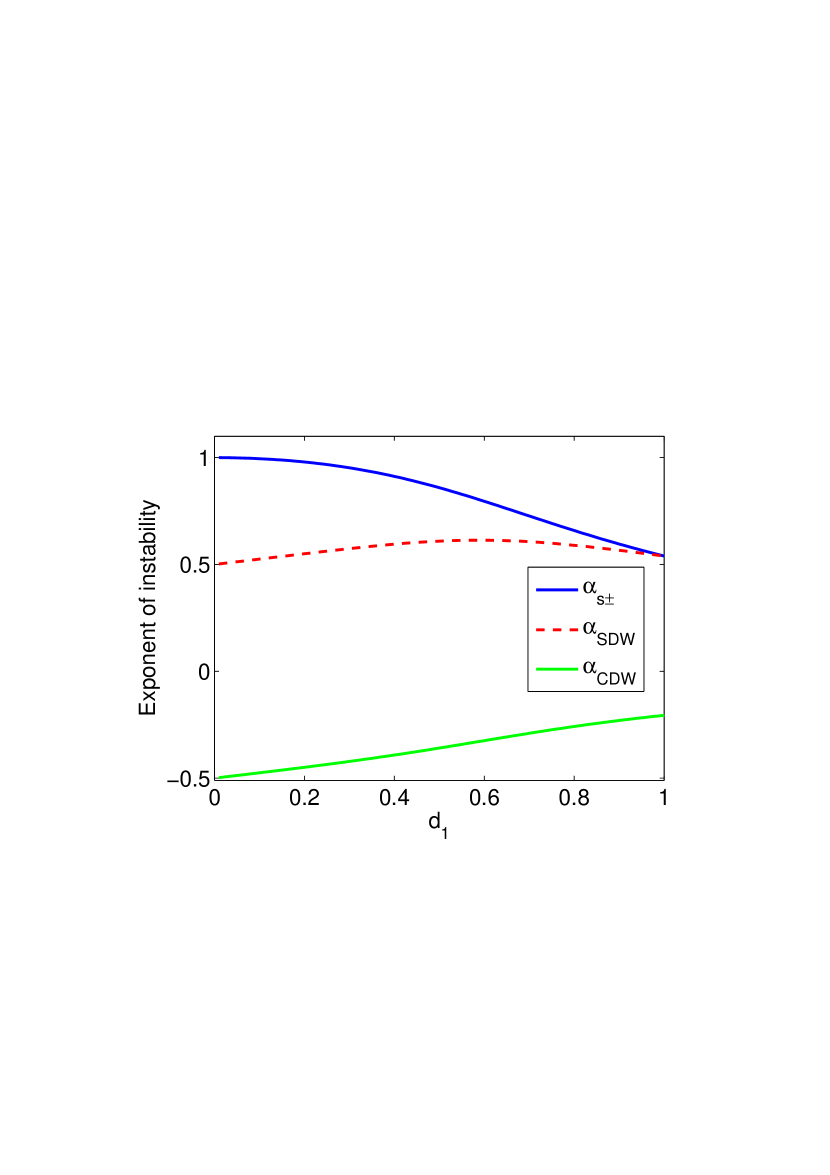
Figure 18: Exponents ($\alpha_{s\pm}$, $\alpha_{SDW}$ and $\alpha_{CDW}$) for different values of the nesting parameter $d_{1}$ calculated near the critical RG scale, where the couplings diverge. The state with the largest exponent wins. SDW and SC are degenerate when $d_{1}=1$ (perfect nesting) and superconductivity wins for all other values of $d_{1}$. CDW is not a competitor for all values of $d_{1}$.

Before moving on, I need to clarify one more point. So far we found that the vertices $\Gamma^{SC}$ and $\Gamma^{SDW}$ diverge and compared the exponents. However, to actually analyze the instability in a particular channel one has to compute fluctuation correction to susceptibility

$$\chi^{i}_{fl}(L)\sim\int d^{2}k(\Gamma^{i})^{2}\Pi_{i}\propto\int^{L}dL^{\prime}\left(\Gamma^{i}(L^{\prime})\right)^{2}$$ (46)

where $\Pi_{i}$ is either $\Pi^{SDW}=\Pi_{ph}$ or $\Pi^{SC}=\Pi_{pp}$ (see Fig 19)

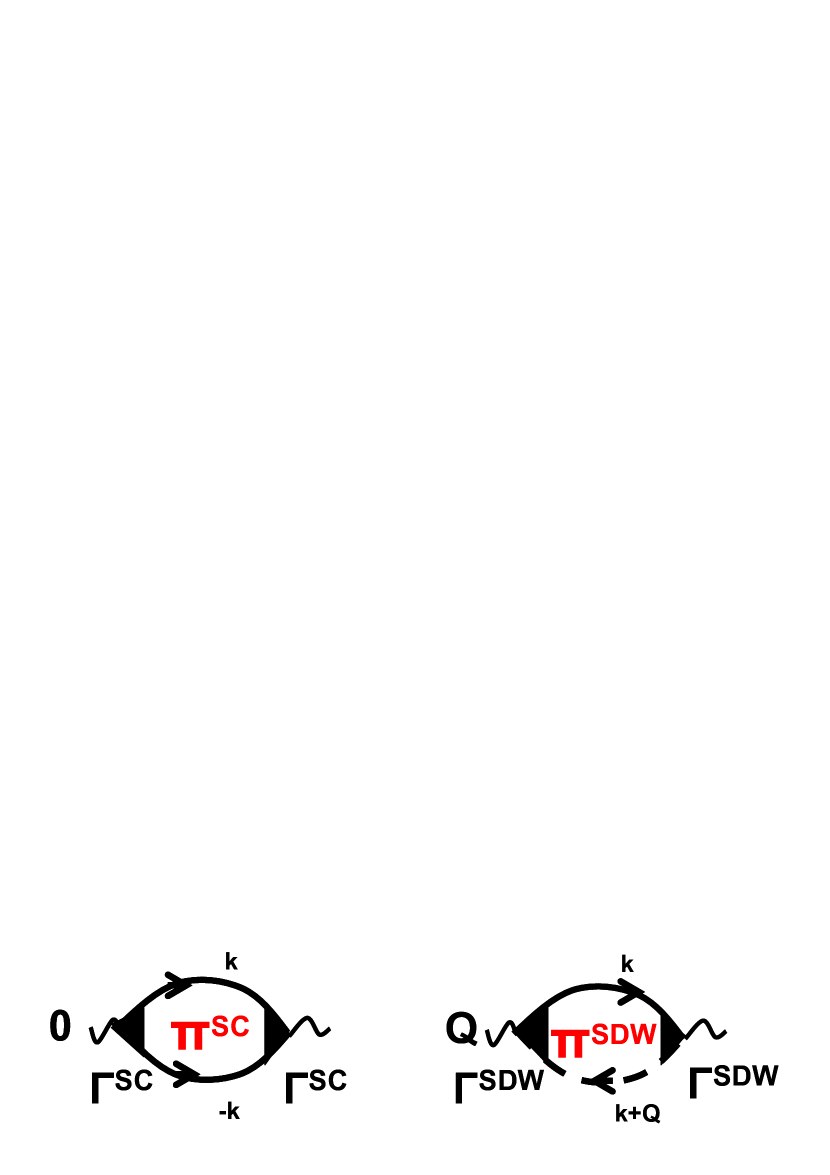
Figure 19: (Left) The fluctuation correction to SC pairing susceptibility. (Right) The fluctuation correction to SDW susceptibility.

The fully renormalized susceptibility in a given channel is

$$\left(\chi^{i}(L)\right)^{-1}=r^{i}_{0}-\chi^{i}_{fl}(L)$$ (47)

where $r^{i}_{0}$ is some bare value of order one. The true instability occurs at $L^{*}$ when $\chi^{i}_{fl}(L^{*})=r^{i}_{0}$. At weak coupling, the critical $L^{*}$ is close to $L_{c}$, and, indeed, the instability occurs first in the channel with the largest exponent for $\Gamma^{i}$. However, we need $\chi^{i}_{fl}(L)$ to diverge at $L_{c}$, otherwise there will no instability at weak coupling Cvetkovic . This requirement sets the condition that the exponent for the corresponding $\Gamma$ must be larger than $1/2$. Fortunately, this condition is satisfied in the two-pocket model. For $d_{1}=1$, this is evident from (V.1). For $d_{1}<1$, the exponent for the SC channel only increases, while the one in SDW channel decreases but still remains larger than $1/2$ as it is evidenced from Fig18 where I plotted the exponents for SC and SDW vertices as a function of $d_{1}$. In the limit $d_{1}\rightarrow 0$,

$$\alpha_{SDW}\approx\frac{1}{2}+\frac{d_{1}}{4}$$ (48)

.

The fact that both $\alpha_{SC}$ and $\alpha_{SDW}$ are larger than $1/2$ implies that in Landau-Ginzburg expansion in powers of SC and SDW order parameters ($\Delta$ and $M$, respectively), not only the prefactor for $\Delta^{2}$ changes sign at $T_{c}$, but also the prefactor for $M^{2}$ term changes sign and becomes negative below some $T_{m}<T_{c}$. This brings in the possibility that at low T SC and SDW orders co-exist. The issue of the co-existence, however, requires a careful analysis of the interplay of prefactors for fourth order terms $M^{4}$, $\Delta^{4}$, and $M^{2}\Delta^{2}$. I do not discuss this specific issue. For details see VVC ; FS .

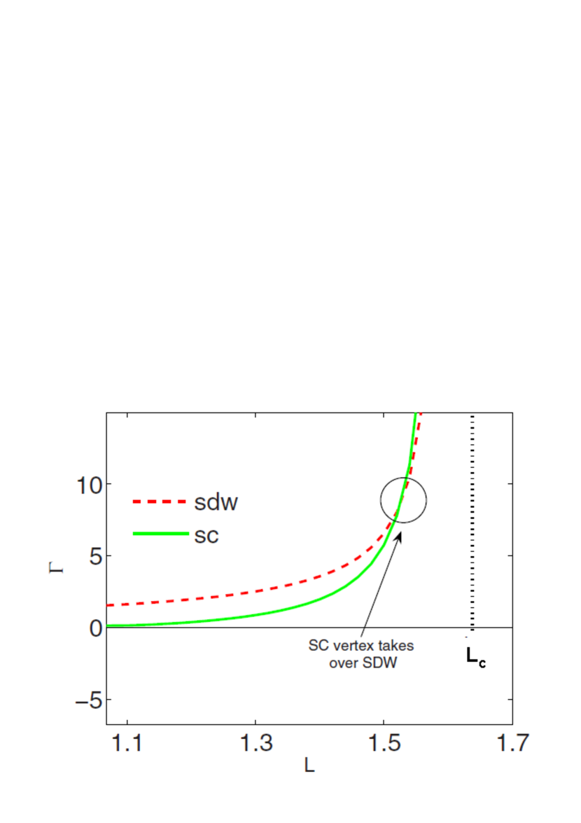
Figure 20: The flow of the SC and SDW vertices with the RG scale. Both diverge at a critical scale, $L_{c}$, but the SC vertex diverges stronger. From Ref. [RG_SM, ].

V.1.1 Multi-pocket models

The interplay between SDW and SC vertices is more involved in more realistic multi-pocket models Fe-pnictides, with several electron and hole pockets. I recall that weakly doped Fe-pnictides have 2 electron pockets and 2-3 hole pockets. In multi-pocket models one needs to introduce a larger number of intra-and inter-pocket interactions and analyze the flow of all couplings to decide which instability is the leading one. This does not provide any new physics compared to what we have discussed, but in several cases the interplay between SC and SDW instabilities becomes such that superconductivity wins already at perfect nesting. In particular, in 3-pocket models (two electron pockets and one hole pockets) the exponent for the SC vertex gets larger than the exponent for the SDW vertex already at $d_{1}=1$. I show the flow of SC an SDW couplings for 3-pocket model in Fig.20. Once $d_{1}$ becomes smaller than one, SC channel wins even bigger compared to SDW channel.

Superconductivity right at zero doping has been detected in several Fe-pnictides, like LaOFeAs and LiFeAs, and it is quite possible that this is at least partly due to the specifics of pRG flow.

V.2 Summary of the pRG approach

I now summarize the key points of the pRG approach

• The SC vertex starts out as repulsive, but it eventually changes sign at some RG scale ($L_{0}$). This happens due to the "push" from SDW channel, which rives rise to upward renormalization of the inter-pocket interaction $g_{3}$.

• Both SDW and SC vertices diverge at RG scale $L_{c}$ which is larger than $L_{0}$. The leading instability is in the channel whose vertex diverges with a larger exponent. At perfect nesting, SDW instability occurs first in 2-pocket model, however in some multi-pocket models SC vertex has a larger exponent that the SDW vertex and SC becomes the leading instability.

• Deviations from perfect nesting (quantified by $d_{1}<1$) act against SDW order by reducing the corresponding exponent. At sufficiently small $d_{1}$ SC instability becomes the leading one.

• The necessary condition for the instability is the diverges of the fluctuating component of the susceptibility. This sets up a condition $\alpha>1/2$, where $\alpha$ is the exponent for the corresponding vertex. For the leading instability, we found $\alpha>1/2$ in all cases. For the subleading instability, $\alpha$ can be either larger or smaller than $1/2$. This affects potential co-existence of the leading and subleading orders at a lower $T$.

VI SDW magnetism and nematic order

For this section, I assume that we are in the range of parameters/dopings, where SDW instability comes first, and consider (i) what kind of SDW order emerges and (ii) the interplay between breaking of $O(3)$ spin-rotational symmetry and breaking of a discrete $C_{4}$ symmetry of rotations on a tetragonal lattice. I consider these two issues one after the other. In the discussions in this section I follow Refs. [Eremin_10, ; rafael_nematic, ; rafael_review, ].

VI.1 Selection of SDW order

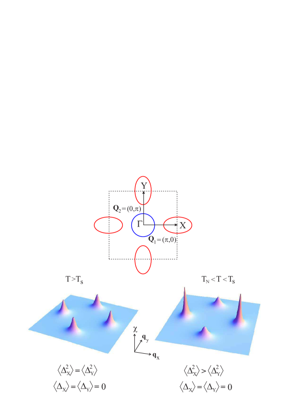
Figure 21: (Color online.) (upper panel) The band-structure with a circular hole pocket at $\Gamma$ and two electron pockets at $X$ and $Y$. The Brillouin zone contains one Fe atom. (lower panels) Static magnetic susceptibility $\chi_{\mathbf{q}}$ across the Brillouin zone for different temperatures. At high temperatures, fluctuations near the two stripe magnetic ordering vectors are equally strong, $\left\langle\Delta_{X}^{2}\right\rangle=\left\langle\Delta_{Y}^{2}\right\rangle$. Above the magnetic ordering temperature $T_{N}$ but below the Ising-nematic ordering temperature $T_{s}$, fluctuations associated with one of the stripe states become stronger (in the figure, $\left\langle\Delta_{X}^{2}\right\rangle>\left\langle\Delta_{Y}^{2}\right\rangle$) and the tetragonal symmetry is broken inside the unit cell. Stronger fluctuations around one ordering vector yield stronger intensity and narrower peaks.

I return to the model I started with, but now with interactions renormalized by pRG contributions from energies lager than $E_{F}$. The only necessary extension we need to make is we need to consider two electron pockets, one at $(0,\pi)$ and another at $(\pi,0)$ in the unfolded Brillouin zone (see Fig.21). To make presentation more simple, we consider only one hole pocket, centered at $(0,0)$. The extension to two (or three) hole pockets is straightforward, but requites care and in some cases leads to new states zlatko ; kang

We need to be a bit more precise and include the ellipticity of electron pockets. Accordingly, we approximate dispersions of fermions near hole and electron pockets by $\varepsilon_{\Gamma,\mathbf{k}}=\varepsilon_{0}-\frac{k^{2}}{2m}-\mu\equiv-\varepsilon$, $\varepsilon_{X,\mathbf{k+Q_{1}}}=\varepsilon-\delta_{0}+\delta_{2}\cos 2\theta$, $\varepsilon_{Y,\mathbf{k+Q_{2}}}=\varepsilon-\delta_{0}-\delta_{2}\cos 2\theta$, where $m_{i}$ denotes the band masses, $\varepsilon_{0}$ is the offset energy, $\mu$ is the chemical potential, $\delta_{0}=2\mu$, $\delta_{2}=\varepsilon_{0}m(m_{x}-m_{y})/(2m_{x}m_{y})$, and $\theta=\tan^{-1}k_{y}/k_{x}$ Vorontsov10 .

I shift the momenta of the fermions near the $X$ and $Y$ Fermi pockets by $\mathbf{Q}_{1}$ and $\mathbf{Q}_{2}$, respectively, i.e. $\varepsilon_{X,\mathbf{k+Q_{1}}}\rightarrow\varepsilon_{X,\mathbf{k}}$, $\varepsilon_{Y,\mathbf{k+Q_{2}}}\rightarrow\varepsilon_{Y,\mathbf{k}}$.

This model has eight fermionic interactions $U_{n}$ (with the same structure as in a 2-pocket model, but now there are four different inter-and intra-pocket interactions involving the two electron pockets). These interactions can be decomposed into the spin density-wave (SDW), the charge density-wave (CDW) and the pairing channels. For magnetism, I keep only the interactions in the spin channel with momenta near $\mathbf{Q}_{1}$ and $\mathbf{Q}_{2}$. This reduces the interacting Hamiltonian to

$$\mathcal{H}_{\mathrm{int}}=-\frac{1}{2}g_{\mathrm{spin}}\sum\limits_{i,\mathbf{q}}\mathbf{s}_{i,\mathbf{q}}\cdot\mathbf{s}_{i,-\mathbf{q}}$$ (49)

where $\mathbf{s}_{i,\mathbf{q}}=\sum_{k}c_{\Gamma,\mathbf{k+q}\alpha}^{\dagger}\bm{\sigma}_{\alpha\beta}c_{i,\mathbf{k}\beta}$ is the electronic spin operator, with Pauli matrices $\bm{\sigma}_{\alpha\beta}$. The coupling $u_{\mathrm{spin}}$ is the combination of density-density and pair-hopping interactions between hole and electron states ($g_{1}$ and $g_{3}$ terms in the same notations as in previous two Sections).

$$g_{1}c_{\Gamma,\alpha}^{\dagger}c_{\Gamma,\alpha}c_{X,\beta}^{\dagger}c_{X,\beta} = -\frac{g_{1}}{2}c_{\Gamma,\alpha}^{\dagger}\bm{\sigma}_{\alpha\beta}c_{X,\beta}\cdot c_{X,\gamma}^{\dagger}\bm{\sigma}_{\gamma\delta}c_{\Gamma,\delta}+(\cdots)$$

$$g_{3}c_{\Gamma,\alpha}^{\dagger}c_{X,\alpha}c_{\Gamma,\beta}^{\dagger}c_{X,\beta} = -\frac{g_{3}}{2}c_{\Gamma,\alpha}^{\dagger}\bm{\sigma}_{\alpha\beta}c_{X,\beta}\cdot c_{X,\gamma}^{\dagger}\bm{\sigma}_{\gamma\delta}c_{\Gamma,\delta}+(\cdots)$$ (50)

where the dots stand for the terms with $\delta_{\alpha,\beta}\delta_{\gamma,\delta}$, which only contribute to the CDW channel. Combining the two contributions for the SDW channel, I find $g_{\mathrm{spin}}=g_{1}+g_{3}$, as in (6). Once $g_{\mathrm{spin}}$ exceeds some critical value (which gets smaller when $\delta_{0}$ and $\delta_{2}$ decrease), static magnetic susceptibility diverges at $(0,\pi)$ and $(\pi,0)$, and the system develops long-range magnetic order. An excitonic-type SDW instability in Fe-pnictides, resulting from the interaction between hole and electron pockets, has been considered by several authors Eremin_10 ; Cvetkovic09 ; Gorkov08 ; Timm09 ; Kuroki08 ; DungHaiLee08 ; Platt08 ; Vorontsov09 ; FS ; Knolle10 .

My strategy is the following: I introduce the two bosonic fields $\bm{\Delta}_{(X,Y)}\propto\sum_{\mathbf{k}}c_{\Gamma,\mathbf{k}\alpha}^{\dagger}\bm{\sigma}_{\alpha\beta}c_{(X,Y),\mathbf{k}\beta}$ for the collective magnetic degrees of freedom, use Hubbard-Stratonovich transformation to get rid of the terms in (49) with four fermions, integrate out the fermions, and obtain a Ginzburg-Landau (GL) action for $\bm{\Delta}_{X}$ and $\bm{\Delta}_{Y}$. I then analyze this action in saddle-point approximation and show that one of the magnetic order parameters - either $\left\langle\bm{\Delta}_{X}\right\rangle$ or $\left\langle\bm{\Delta}_{Y}\right\rangle$ - becomes non-zero in the magnetically ordered state. This leads to stripe-type SDW order in which spins are ordered ferromagnetically in one direction and antiferromagnetically in the other, i.e. the ordering momentum is either $(\pi,0)$ or $(0,\pi)$. I then show that another state, in which $\left\langle\bm{\Delta}_{X}\right\rangle$ or $\left\langle\bm{\Delta}_{Y}\right\rangle$ emerge simultaneously, may occur at a higher doping osborn . The same tendency occurs in systems like Ba(Fe_1-xMn_x)₂As₂, where the local Mn moments interact with the Fe conduction electrons rafael_last .

VI.1.1 The action in terms of $\bm{\Delta}_{X}$ and $\bm{\Delta}_{Y}$

A straightforward way to obtain the action in terms of $\left\langle\bm{\Delta}_{X}\right\rangle$ and $\left\langle\bm{\Delta}_{Y}\right\rangle$ is to start with the fermionic Hamiltonian $\mathcal{H}=\mathcal{H}_{\mathrm{0}}+\mathcal{H}_{\mathrm{int}}$ and write the partition function as the integral over Grassmann variables:

$$Z\propto\int dc_{i,\mathbf{k}}dc_{i,\mathbf{k}}^{\dagger}\mathrm{e}^{-\beta\mathcal{H}}$$ (51)

and then decouple the quartic term in fermionic operators using the Hubbard-Stratonovich transformation:

$$\mathrm{e}^{\frac{ax^{2}}{2}}=\frac{1}{\sqrt{2\pi a}}\int dy\,\mathrm{e}^{\left(-\frac{y^{2}}{2a}+yx\right)}$$ (52)

where, in our case, $x=\mathbf{s}_{i,\mathbf{0}}=\sum_{k}c_{\Gamma,\mathbf{k}\alpha}^{\dagger}\bm{\sigma}_{\alpha\beta}c_{(X,Y),\mathbf{k}\beta}$ and $y=\bm{\Delta}_{(X,Y)}$. One can then integrate Eq. (51) over fermionic variables using the fact that after the Hubbard-Stratonovich transformation the effective action becomes quadratic with respect to the fermionic operators. The result of the integration is recast back into the exponent and the partition function is expressed as:

$$Z\propto\int d\bm{\Delta}_{X}d\bm{\Delta}_{Y}\mathrm{e}^{-S_{\mathrm{eff}}\left[\bm{\Delta}_{X},\bm{\Delta}_{Y}\right]}$$ (53)

If relevant $\bm{\Delta}_{X}$ and $\bm{\Delta}_{Y}$ are small, which I assume to hold even if the magnetic transition is first-order (I present the conditions on the parameters below), one can expand $S_{\mathrm{eff}}\left[\bm{\Delta}_{X},\bm{\Delta}_{Y}\right]$ in powers of $\bm{\Delta}_{X}$ and $\bm{\Delta}_{Y}$ and obtain the Ginzburg-Landau type of action for the order parameters $\bm{\Delta}_{X},\bm{\Delta}_{Y}$. For uniform $\bm{\Delta}_{i}$, the most generic form of $S_{\mathrm{eff}}\left[\bm{\Delta}_{X},\bm{\Delta}_{Y}\right]$ is

$$S_{\mathrm{eff}}\left[\bm{\Delta}_{X},\bm{\Delta}_{Y}\right] = r_{0}\left(\bm{\Delta}_{X}^{2}+\bm{\Delta}_{Y}^{2}\right)+\frac{u}{2}\left(\bm{\Delta}_{X}^{2}+\bm{\Delta}_{Y}^{2}\right)^{2}$$ (54)

$$-\frac{g}{2}\left(\bm{\Delta}_{X}^{2}-\bm{\Delta}_{Y}^{2}\right)^{2}+v\left(\bm{\Delta}_{X}\cdot\bm{\Delta}_{Y}\right)^{2}$$

Carrying out this procedure, one obtains the coefficients $r_{0}$, $u$, $g$, and $v$ in terms of the non-interacting fermionic propagators convoluted with Pauli matrices. The coefficient $v$ vanishes in our model because of the anti-commutation property of the Pauli matrices: $\sigma^{i}\sigma^{j}+\sigma^{j}\sigma^{i}=0$ for $i\neq j$. To get a non-zero $v$, one needs to include direct interactions between the two electron pockets Eremin_10 . The other three prefactors are expressed via fermionic propagators $G_{j,\mathbf{k}}^{-1}=i\omega_{n}-\xi_{j,\mathbf{k}}$ as

$$r_{0} = \frac{2}{g_{\mathrm{spin}}}+2\int_{k}G_{\Gamma,k}G_{X,k}$$

$$u = \frac{1}{2}\int_{k}G_{\Gamma,k}^{2}\left(G_{X,k}+G_{Y,k}\right)^{2}$$

$$g = -\frac{1}{2}\int_{k}G_{\Gamma,k}^{2}\left(G_{X,k}-G_{Y,k}\right)^{2}$$ (55)

where $\int_{k}=T\sum_{n}\int\frac{d^{d}k}{\left(2\pi\right)^{d}}$ and $k=\left(\mathbf{k},\omega_{n}\right)$, with momentum $\mathbf{k}$ and Matsubara frequency $\omega_{n}=\left(2n+1\right)\pi T$. Similar coefficients were found in Ref. Brydon11 , which focused on the magnetic instabilities in a two-band model. Near $T_{N,0}$ one can expand $r_{0}$ as $r_{0}=a(T-T_{N,0})$, with $a>0$. Evaluating the integrals with the products of the Green’s functions, we obtain

$$u \approx \frac{7\zeta\left(3\right)N_{F}}{4\pi^{2}T^{2}}$$

$$g \approx 0.024u\left(\frac{\varepsilon_{0}\delta m}{T}\right)^{2}$$ (56)

for $\delta m\ll T/\varepsilon_{0}\ll 1$. The crucial result for our consideration is that $g$ is positive for any non-zero ellipticity.

The action $S_{\mathrm{eff}}$ is exact and includes all fluctuations of the two bosonic fields. Fluctuations need to be included for the analysis of a potential nematic order (see below), but the type of SDW can be analyzed already in the mean-field approximation (see Refs Eremin_10 ; rafael_nematic for justification.) Solving for the minimum of $S_{\mathrm{eff}}\left[\bm{\Delta}_{X},\bm{\Delta}_{Y}\right]$ in Eq. (54), we find that, when $g=0$, the ground state has a huge degeneracy because any configuration $\bm{\Delta}=\left\langle\bm{\Delta}_{X}\right\rangle\mathrm{e}^{i\mathbf{Q}_{1}\cdot\mathbf{r}}+\left\langle\bm{\Delta}_{Y}\right\rangle\mathrm{e}^{i\mathbf{Q}_{1}\cdot\mathbf{r}}$ with $\left\langle\bm{\Delta}_{X}\right\rangle^{2}+\left\langle\bm{\Delta}_{Y}\right\rangle^{2}=-r_{0}/u$ minimizes $\tilde{S}_{\mathrm{eff}}$. A non-zero $g$ gives rise to the additional coupling $2g\Delta_{X}^{2}\Delta_{Y}^{2}$, which breaks this degeneracy. For a positive $g$, this term favors the states in which only one order parameter has a nonzero value, i.e. configurations with either $\left\langle\bm{\Delta}_{X}\right\rangle\neq 0$ or $\left\langle\bm{\Delta}_{X}\right\rangle\neq 0$, but not both. These are stripe phases, in which spins order ferromagnetically along one direction and antiferromagnetically along the other one.

For larger dopings, recent calculations osborn have shown that $g$ may change sign and become negative. Then the SDW phase does not break $C_{4}$ symmetry. The transformation from a stripe SDW state to a state which preserves $C_{4}$ symmetry has recently been observed in Ba_1-xNa_xFe₂As₂ near the end of the SDW region osborn .

VI.2 pre-emptive spin-nematic order

I now analyze a possibility that $Z_{2}$ symmetry between $X$ and $Y$ directions gets broken before the system develops a stripe SDW order. To analyze this possibility, I include fluctuations of the $\bm{\Delta}_{X,Y}$ fields, introduce the collective Ising-nematic bosonic variable $\phi\propto\Delta_{X}^{2}-\Delta_{Y}^{2}$ together with $\psi\propto\bm{\Delta}_{X}^{2}+\bm{\Delta}_{Y}^{2}$, integrate over $\bm{\Delta}_{X}$ and $\bm{\Delta}_{Y}$, and obtain an effective action in terms of $\phi$ and $\psi$. I analyze this action and check whether the system develops an instability towards $\left\langle\phi\right\rangle\neq 0$ before $\left\langle\bm{\Delta}_{X}\right\rangle$ or $\left\langle\bm{\Delta}_{Y}\right\rangle$ becomes non-zero (see Fig. 21).

That the action (54) can potentially lead to a preemptive Ising-nematic instability is evident from the presence of the term $g\left(\Delta_{X}^{2}-\Delta_{Y}^{2}\right)^{2}$, which can give rise to an ordered state with $\left\langle\Delta_{X}^{2}\right\rangle-\left\langle\Delta_{Y}^{2}\right\rangle\neq 0$ in a way similar to how the $\bm{s}_{i,\mathbf{q}}\bm{s}_{i,-\mathbf{q}}$ term in the Hamiltonian (49) gives rise to a state with non-zero $\left\langle\bm{s}_{i,0}\right\rangle\neq 0$. The pre-emptive Ising-nematic instability, however, does not appear in the mean-field approximation simply because when magnetic fluctuations are absent, a non-zero $\left\langle\Delta_{i}^{2}\right\rangle\neq 0$ appears simultaneously to $\left\langle\Delta_{i}\right\rangle\neq 0$, once $r_{0}$ changes sign. However, it may well happen once we go beyond mean-field and include magnetic fluctuations.

To study a potential preemptive $Z_{2}$ transition, I need to introduce collective variables of the fields $\bm{\Delta}_{X}$ and $\bm{\Delta}_{Y}$. Let me introduce auxiliary scalar fields $\phi$ for $\bm{\Delta}_{X}^{2}-\bm{\Delta}_{Y}^{2}$ and $\psi$ for $\bm{\Delta}_{X}^{2}+\bm{\Delta}_{Y}^{2}$. The field $\psi$ always has a non-zero expectation value $\left\langle\psi\right\rangle\neq 0$, which describes Gaussian corrections to the magnetic susceptibility $\chi_{i,q}^{-1}$ in Eq. 58. Meanwhile, the field $\phi$ may or may not have a non-zero expectation value. If it does, it generates a non-zero value of $\left\langle\bm{\Delta}_{X}^{2}-\bm{\Delta}_{Y}^{2}\right\rangle$ and the system develops an Ising-nematic order.

The effective action in terms of $\phi$ and $\psi$ is obtained by using again the Hubbard-Stratonovich transformation of Eq. (51), but this time the variable $x$ is either $\psi\propto\Delta_{X}^{2}+\Delta_{Y}^{2}$ or $\phi\propto\Delta_{X}^{2}-\Delta_{Y}^{2}$. Applying this transformation and integrating over fluctuating fields $\Delta_{X}$ and $\Delta_{Y}$, I obtain the effective action in terms on $\phi$ and $\psi$ in the form

$$S_{\mathrm{eff}}\left[\phi,\psi\right]=\int_{q}\left\{\frac{\phi^{2}}{2g}-\frac{\psi^{2}}{2u}+\frac{3}{2}\log\left[\left(\chi_{q}^{-1}+\psi\right)^{2}-\phi^{2}\right]\right\}$$ (57)

As it is customary for the analysis of fluctuating fields $\Delta_{X}$ and $\Delta_{Y}$, we extended the mass term $r_{0}$ to include spatial and time variations of $\Delta_{X,Y}$:

$$r_{0}\rightarrow\chi_{i,q}^{-1}=r_{0}+\gamma\left|\nu_{n}\right|+q^{2}$$ (58)

where $\nu_{n}=2\pi Tn$ is the bosonic Matsubara frequency.

This action can be straightforwardly analyzed in the saddle-point approximation $\partial S_{\mathrm{eff}}\left[\phi,\psi\right]/\partial\phi=\partial S_{\mathrm{eff}}\left[\phi,\psi\right]/\partial\psi=0$ (for justification see Ref. rafael_nematic ). Differentiating, I obtain two non-linear coupled equations for $\phi$ and $\psi$:

$$\frac{\psi}{u} = \int_{q}\frac{r_{0}+\psi+q^{2}+\gamma|\nu_{n}|}{\left(r_{0}+\psi+q^{2}+\gamma|\nu_{n}|\right)^{2}-\phi^{2}}$$

$$\frac{\phi}{g} = \int_{q}\frac{\phi}{\left(r_{0}+\psi+q^{2}+\gamma|\nu_{n}|\right)^{2}-\phi^{2}}$$ (59)

The full solution of these equations at various temperatures and in different dimensions is presented in Ref. rafael_nematic . The key point is that, for positive $g$, $\phi$ becomes non-zero at a higher temperature $(T_{n})$ than the one ($T_{sdw})$ at which SDW order sets in. In the interval $T_{n}>T>T_{sdw}$, $\left\langle\bm{\Delta}_{X}^{2}-\bm{\Delta}_{Y}^{2}\right\rangle$ becomes non-zero, while $\left\langle\bm{\Delta}_{X}\right\rangle=\left\langle\bm{\Delta}_{Y}^{2}\right\rangle=0$. Such an order breaks $C_{4}$ lattice symmetry down to $C_{2}$ and is often called Ising-nematic order.

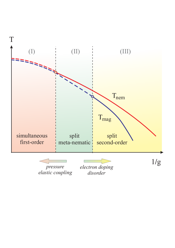
Figure 22: Evolution of the character of the magnetic and nematic transitions in the spin-driven nematic theory. The control parameter is the inverse nematic coupling $g$, which changes as function of various control parameters within an itinerant scenario (arrows). Second-order (first-order) lines are denotes by solid (dashed) lines. Regions (I)-(III) correspond to those of the phase diagram in Fig. 1. The arrows show how the nematic order parameter $g$ is expected to evolve with doping, disorder, pressure, and elastic coupling. From [rafael_nematic, ].

In Fig. 22 I present the phase diagram for anisotropic 3D system. The transition to an Ising-nematic state can be either second-order, or first order. A strong first-order nematic transition may instantly induce SDW order.

VI.3 consequences of the Ising-nematic order

Because spin-nematic order breaks $C_{4}$ lattice rotational symmetry, it couples linearly to any other parameter which breaks the same symmetry, such as orbital and structural order parameters. Then, once spin-nematic order becomes non-zero, it acts as "external field" to the two other parameters and induces non-zero values of both of them. As a result, below $T_{n}$ the fermionic dispersion becomes anisotropic, the occupations of $d_{xz}$ and $d_{yz}$ orbitals become non-equal, and also the lattice constants $a$ and $b$ along the $x$ and $y$ directions of the Fe-plane, respectively, become non-equal. I refrain to discuss this issue in more detail here and direct a reader to a recent review rafael_review . The development of the Ising-nematic order also gives rise to an increase of the magnetic correlation length, what in turn gives rise to a pseudo-gap-type behavior of the fermionic spectral function.

VII The structure of the superconducting gap

I now turn to superconductivity. Like I did for SDW order, I assume that renormalizations captured within pRG are already included into consideration and consider an effective low-energy model with effective pairing interactions in the band basis. In the discussions in this Section I follow Refs. [ch_annual, ; cee, ; cvv, ; maiti_rev, ; maiti_book, ; RG_SM, ; maiti_kor, ; maiti_11, ].

VII.1 The structure of $s-$wave and $d-$wave gaps in a multi-band SC - general reasoning

In previous sections I assumed that the interactions in the particle-particle channel (the dressed $G_{3}$ and $G_{4}$ terms) are independent on the angles along the hole and electron FSs. In this situation, the only option is an $s-$wave gap, which changes sign between the FSs, but is a constant along each FS. Now I consider realistic models in which the interactions in the band basis are obtained from the underlying multi-orbital model. These interactions generally depend on locations of fermions along the FS.

I first display general arguments on what should be the form of the gap in different symmetries and on different FSs. I show that an $s-$wave gap generally has angle dependence and may even have nodes, while a d-wave gap, which is normally assumed to have nodes, may in fact be nodeless on electron FSs.

A generic low-energy BCS-type model in the band basis is described by

$${\cal H}=\sum_{i,{\bf k}}\epsilon_{i}({\bf k})a^{\dagger}_{i{\bf k}}a_{i{\bf k}}+\sum_{i,j,{\bf k},{\bf p}}U_{i,j}({\bf k},{\bf p})a^{\dagger}_{i{\bf k}}a^{\dagger}_{i-{\bf k}}a_{j{\bf p}}a_{j-{\bf p}}$$ (60)

The quadratic term describes low-energy excitations near hole and electron FSs, labeled by $i$ and $j$, and the four-fermion term describes the scattering of a pair $(k\uparrow,-k\downarrow)$ on the FS $i$ to a pair $(p\uparrow,-p\downarrow)$ on the FS $j$. These interactions are either intra-pocket interactions (hole-hole $U_{h_{i}h_{i}}$ or electron-electron $U_{e_{i}e_{i}}$ ), or inter-pocket interactions (hole-electron $U_{e_{j}h_{i}}$, hole-hole $U_{h_{i}\neq h_{j}}$, and electron-electron $U_{e_{i}\neq e_{j}}$).

Assume for simplicity that the frequency dependence of $\Gamma$ can be neglected and low-energy fermions are Fermi-liquid quasiparticles with Fermi velocity $v_{k_{F}}$. In this situation, the gap $\Delta(k)$ also doesn’t depend on frequency, and to obtain $T_{c}$ one has to solve the eigenfunction/eigenvalue problem:

$$\lambda_{i}\Delta_{i}(k)=-\int\frac{dp_{\parallel}}{4\pi^{2}v_{{\bf p}_{F}}}\Gamma({\bf k}_{F},{\bf p}_{F})\Delta_{i}(p)$$ (61)

where $\Delta_{i}$ are eigenfunctions and $\lambda_{i}$ are eigenvalues. The system is unstable towards pairing if one or more $\lambda_{i}$ are positive. The corresponding $T_{c,i}$ scale as $T_{c,i}=\Lambda_{i}e^{-1/\lambda_{i}}$. Although $\Lambda_{i}$ are generally different for different $i$, the exponential dependence on $1/\lambda_{i}$ implies that, most likely, the solution with the largest positive $\lambda_{i}$ emerges first and establish the pairing state, at least immediately below $T_{c}$.

Like I discussed in the Introduction, the pairing interaction $U(k,p)$ can be decomposed into representations of the tetragonal space group (one-dimensional representations are $A_{1g}$, $B_{1g}$, $B_{2g}$, and $A_{2g}$). Basis functions from different representations do not mix, but each contains infinite number of components. For example, $s-$wave pairing corresponds to fully symmetric $A_{1g}$ representation, and the $s-$wave ($A_{1g}$) component of $U(k,p)$ can be quite generally expressed as

$$U^{(1g)}(k,p)=U_{s}(k,p)=\sum_{m,n}A^{s}_{mn}\Psi^{s}_{m}(k)\Psi^{s}_{n}(p)$$ (62)

where $\Psi^{s}_{m}(k)$ are the basis functions of the A_1g symmetry group: $1$, $\cos k_{x}\cos k_{y}$, $\cos k_{x}+\ cosk_{y}$, etc, and $A^{s}_{mn}$ are coefficients. Suppose that $k$ belongs to a hole FS and is close to $k=0$. Expanding any wave function with A_1g symmetry near $k=0$, one obtains along $|{\bf k}|=k_{F}$,

$$\Psi^{s}_{m}(k)=a_{m}+b_{m}\cos 4\phi_{k}+c_{m}\cos 8\phi_{k}+...$$ (63)

where $\phi_{k}$ is the angle along the hole FS (which is not necessary a circle). Similarly, for $B_{1g}$ representation the wave-functions are $\cos k_{x}-\cos k_{y}$, $cos2k_{x}-cos2k_{y}$, etc, and expanding them near $k=0$ one obtains

$$\Psi^{d}_{m}(k)=a^{*}_{m}\cos 2\phi_{k}+b^{*}_{m}\cos 6\phi_{k}+c^{*}_{m}\cos 10\phi_{k}+...$$ (64)

There are no fundamental reasons to expect that $b_{m},\leavevmode\nobreak\ c_{m}$ or $b^{*}_{m},c^{*}_{m}$ are much smaller than $a_{m}$ or $a^{*}_{m}$, but sub-leading terms are often small numerically. I assume that this is the case and neglect subleading terms, i.e., assume that $s-$wave interaction between fermions on the hole FSs can be approximated by an angle-independent $U^{s}_{h_{i}h_{j}}(k,p)\equiv U_{h_{i}h_{j}}$ ($h_{i}$ label different hole FSs), while $d-$wave ($B_{1g}$) interaction can be approximated by $U^{d}_{h_{i}h_{j}}(k,p)={\tilde{U}}_{h_{i}h_{j}}\cos 2\phi_{k}\cos 2\phi_{p}$.

The situation changes, however, when I consider the pairing component involving fermions from electron FSs. Suppose that $k$ are still near the center of the BZ, but $p$ are near one of the two electron FSs, say the one centered at $(0,\pi)$. Consider all possible $\Psi_{n}(p)$ with $A_{1g}$ symmetry A simple experimentation with trigonometry shows that there are two different subsets of basis functions:

$${\text{s}ubset}\leavevmode\nobreak\ I:1,\leavevmode\nobreak\ \cos{p_{x}}\cos{p_{y}},\leavevmode\nobreak\ \cos{2p_{x}}+\cos{2p_{y}}...$$

$${\text{s}ubset}\leavevmode\nobreak\ II:\cos{p_{x}}+\cos{p_{y}},\leavevmode\nobreak\ \cos{3p_{x}}+\cos{3p_{y}}...$$ (65)

For a circular FS centered at $(0,\pi)$, the functions from subset I can be again expanded in series of $\cos 4l\phi_{p}$ with integer $l$. The functions from subset II are different – they all vanish at $(0,\pi)$ and are expanded in series of $\cos(2\phi_{p}+4l\phi_{p})$ (the first term is $\cos 2\phi_{p}$, the second is $\leavevmode\nobreak\ \cos 6\phi_{p}$, etc). For elliptic FS $\cos 4l\phi_{p}$ and $\cos(2\phi_{p}+4l\phi_{p})$ terms appear in both subsets. In either case, the total

$$\Psi^{s}_{m}(p) = {\bar{a}}_{m}+{\bar{b}}_{m}\cos 4\phi_{p}+{\bar{c}}_{m}\cos 8\phi_{p}+...$$ (66)

$$+{\bar{\bar{a}}}_{m}\cos 2\phi_{p}+{\bar{\bar{b}}}_{m}\cos 6\phi_{p}+{\bar{\bar{c}}}_{m}\cos 10\phi_{k}+...$$

For the other electron FS, $\Psi^{s}_{m}(p)$ is the same, but momentum components $p_{x}$ and $p_{y}$are interchanged, hence the sign of all $\cos(2\phi+4l\phi_{p})$ components changes.

Let’s make the same approximation as before and neglect all components with $l>0$. Then

$$\Psi^{s}_{m}(p)={\bar{a}}_{m}\pm{\bar{\bar{a}}}_{m}\cos 2\phi_{p}$$ (67)

where the upper sign is for one electron FS and the lower for the other. It is essential that the angle-independent term and the $\cos 2\phi_{p}$ term have to be treated on equal footing because each is the leading term in the corresponding series. Combing (67) with the fact that $\Psi^{s}_{m}(k)$ can be approximated by a constant, we obtain a generic form of the $s-$wave component of the interaction between fermions near hole and electron FSs

$$U^{s}_{e_{1},h_{i}}(k,p) = U_{e,h_{i}}\left(1+2\alpha_{e,h}\cos 2\phi_{p_{e1}}+...\right)$$

$$U^{s}_{e_{2},h_{i}}(k,p) = U_{e,h_{i}}\left(1-2\alpha_{e,h}\cos 2\phi_{p_{e2}}+....\right)$$ (68)

where dots stand for $\cos{4\phi_{k}},\cos{4\phi_{p}},\cos{6\phi_{p}}$, etc terms.

By the same reasoning, $s-$wave components of inter-pocket and intra-pocket interactions between fermions from electron FSs are

$$U^{s}_{e_{1},e_{1}}(k,p) = U_{e,e}\left(1+2\alpha_{ee}\left(\cos 2\phi_{k_{e1}}+\cos 2\phi_{p_{e1}}\right)\right.$$

$$+4\beta_{ee}\cos 2\phi_{k_{e1}}\cos 2\phi_{p_{e1}}+...$$

$$U^{s}_{e_{2},e_{2}}(k,p) = U_{e,e}\left(1-2\alpha_{ee}\left(\cos 2\phi_{k_{e2}}+\cos 2\phi_{p_{e2}}\right)\right.$$

$$+4\beta_{ee}\cos 2\phi_{k_{e2}}\cos 2\phi_{p_{e2}}+...$$

$$U^{s}_{e_{1},e_{2}}(k,p) = U_{e,e}\left(1+2\alpha_{ee}\left(\cos 2\phi_{k_{e1}}-\cos 2\phi_{p_{e2}}\right)\right.$$ (69)

$$-4\beta_{ee}\cos 2\phi_{k_{e1}}\cos 2\phi_{p_{e2}}+...$$

Once the pairing interaction has the form of Eqs. (68) and (69), the gaps along the hole FSs are angle-independent (modulo $\cos 4\phi$ terms), but the gaps along the two electron FSs are of the form

$$\Delta^{(s)}_{e}(k)=\Delta_{e}\pm\bar{\Delta}_{e}\cos 2\phi_{k}.$$ (70)

When $\bar{\Delta}_{e}$ is small compared to $\Delta_{e}$, the angle dependence is weak, but when $|\bar{\Delta}_{e}|>|\Delta_{e}|$, $s-$wave gaps have nodes at “accidental” values of $\phi$, which differ between the two electron FSs.

A similar consideration holds for $d_{x^{2}-y^{2}}$ gap. Within the same approximation of leading angular momentum harmonics, we have

$$U^{d}_{e_{1},h_{i}}(k,p) = {\tilde{U}}_{e,h_{i}}\cos 2\phi_{h_{i}}\left(1+{\tilde{\alpha}}_{e,h}\cos 2\phi_{p_{e1}}\right)+...$$

$$U^{d}_{e_{2},h_{i}}(k,p) = {\tilde{U}}_{e,h_{i}}\cos 2\phi_{h_{i}}\left(-1+{\tilde{\alpha}}_{e,h}\cos 2\phi_{p_{e2}}\right)+...$$ (71)

and

$$U^{d}_{e_{1},e_{1}}(k,p) = {\tilde{U}}_{e,e}\left(1+2\alpha_{ee}\left(\cos 2\phi_{k_{e1}}+\cos 2\phi_{p_{e1}}\right)\right.$$

$$+4\beta_{ee}\cos 2\phi_{k_{e1}}\cos 2\phi_{p_{e1}}+...$$

$$U^{d}_{e_{2},e_{2}}(k,p) = {\tilde{U}}_{e,e}\left(1-2\alpha_{ee}\left(\cos 2\phi_{k_{e2}}+\cos 2\phi_{p_{e2}}\right)\right.$$

$$+4\beta_{ee}\cos 2\phi_{k_{e2}}\cos 2\phi_{p_{e2}}+...$$

$$U^{d}_{e_{1},e_{2}}(k,p) = {\tilde{U}}_{e,e}\left(-1-2\alpha_{ee}\left(\cos 2\phi_{k_{e1}}-\cos 2\phi_{p_{e2}}\right)\right.$$ (72)

$$+4\beta_{ee}\cos 2\phi_{k_{e1}}\cos 2\phi_{p_{e2}}+...$$

The solution of the gap equation then yields the gap in the form

$$\Delta^{(d)}_{h}(k)={\tilde{\Delta}}_{h}\cos 2\phi_{k}$$

$$\Delta^{(d)}_{e}(k)=\pm{\tilde{\Delta}}_{e}+\bar{{\tilde{\Delta}}}_{e}\cos 2\phi_{k}.$$ (73)

Along the hole FS, the gap behaves as a conventional $d-$wave gap with 4 nodes along the diagonals. Along electron FSs, the two gaps differ in the sign of the angle-independent terms, and have in-phase $\cos 2\phi$ oscillating components. When $\bar{{\tilde{\Delta}}}_{e}<<{\tilde{\Delta}}_{e}$ the two electron gaps are simply “plus” and “minus” gaps, but when $\bar{{\tilde{\Delta}}}_{e}>{\tilde{\Delta}}_{e}$, each has accidental nodes, again along different directions on the two electron FSs.

We see therefore that the geometry of the FSs in FeSCs affects the gap structure in quite fundamental way: because electron FSs are centered at the $k$ points which are not along BZ diagonals, $s-$wave gaps on these FSs have $\cos 2\phi$ oscillations which one normally would associate with a $d-$wave symmetry, and $d-$wave gaps have constant (plus-minus) components which one would normally associate with an $s-$wave symmetry. When these “wrong” components are large, the gaps have accidental nodes. These nodes may be present or absent for both $s-$wave and $d-$wave gaps.

An $s-$wave gap with nodes in one of the “exotic” options offered by the electronic structure of FeSCs. Another “exotic” option is a $d-$wave state without nodes. In heavily electron-doped FeSCs, hole states are gapped, and only electron FSs remain. The $d-$wave gaps on these two FSs have no nodes if $\cos 2\phi$ oscillation component is smaller than a constant term, hence the system will display a behavior typical for a fully gapped SC despite that the gap actually has a d-wave symmetry. There are even more exotic options offered by the actual three-dimensionality of the electronic structure and/or the hybridization of the electron FSs due to interaction via a pnictide/chalcogen, Refs. [3D, ; mazin, ; khodas, ; khodas_3, ].

A generic analysis of the eigenvalue/eigenfunction problem, Eq. (61), reduces to the set of either four (or five) coupled equations in either s-wave or d-wave channels: two (or three) $\Delta$’s are the gaps on the hole FSs, and two other $\Delta$’s are angle-independent and $\cos 2\phi$ components of the gaps on the electron FSs. Accordingly, there are either four or five different $\lambda_{s}$ and $\lambda_{d}$.

VII.1.1 Generic condition for a non-zero $T_{c}$.

Before I analyze specific cases of $4\times 4$ and $5\times 5$ gap equations, I consider the issue whether in the presence of angular dependence of the interactions its is still required for superconductivity that the inter-pocket interaction $u_{he}$ must exceed the threshold set by intra-pocket hole-hole and electron-electron interactions. Interestingly enough, this may no longer be necessary. To illustrate this, consider the case of an $s-$wave pairing in a four-pocket model and assume for simplification that only one hole pocket is relevant to the pairing. Then the eigenvalue problem reduces to the set of three equations for $\Delta_{h}$, $\Delta_{e}$, and ${\bar{\Delta}}_{e}$ ($\Delta_{e}(k)=\Delta_{e}+{\bar{\Delta}}_{e}\cos{2\phi_{k}}$). Solving the set, we find three solutions $\lambda^{s}_{i}$ ($i=1,2,3$). In the absence of $\cos 2\phi$ terms in $\Gamma_{ij}(k,p)$, $\lambda^{s}_{3}=0$, and $\lambda^{s}_{1,2}$ are given by

$$\lambda^{s}_{1,2}=\frac{-(u_{hh}+2u_{ee})\pm\sqrt{(u_{hh}-2u_{ee})^{2}+8u^{2}_{he}}}{2}$$ (74)

I remind that $u_{ij}=U_{ij}N_{0}$, where $N_{0}$ is the density of states. Obviously, $u_{he}$ has to exceed a threshold, otherwise $\lambda^{s}_{1,2}<0$. Once the angle dependent terms in (68-69) become non-zero, $\lambda^{s}_{3}$ also becomes non-zero, and its sign depends on the interplay between $\alpha_{he}$, $\alpha_{ee}$, and $\beta_{ee}$. In particular, when $u^{2}_{he}<u_{ee}u_{hh}$ (and, hence, $\lambda_{1,2}<0$), $\lambda^{s}_{3}$ is positive or negative depending on whether or not $A>0$, where

$$A=4u_{ee}u_{hh}\left(\alpha^{2}_{ee}-\beta_{ee}\right)+u^{2}_{he}\left(\alpha^{2}_{he}+2\beta_{ee}-3\alpha_{he}\alpha_{ee}\right)$$ (75)

When the angle-dependence of the electron-electron interaction can be neglected, i.e., $\alpha_{ee}=\beta_{ee}=0$, $\lambda^{s}_{3}>0$ no matter what is the ratio of $u^{2}_{he}$ and $u_{ee}u_{hh}$. In particular, for $u_{hh}u_{ee}>u^{2}_{he}$ and $\alpha_{he}<<1$,

$$\lambda^{s}_{3}=\alpha^{2}_{he}\frac{2u^{2}_{he}u_{hh}}{u_{hh}u_{ee}-u^{2}_{he}}>0$$ (76)

In other words, for one of $s-$wave solutions, $\lambda^{s}>0$ even if intra-pocket repulsions are the largest. The full solution of the $3\times 3$ set with $\alpha_{ee}=\beta_{ee}=0$ shows that two $\lambda$’s are repulsive and one is attractive for arbitrary $u^{2}_{he}/u_{ee}u_{hh}$. When the ratio is small, the attractive solution is close to (76), when the ratio is large, the attractive solution is close to $\lambda^{s}_{1}$ in (74). I illustrate this in Fig. 23

$\begin{array}[]{cc}\includegraphics[width=216.81pt]{SC_vrtcs_ap4_annual.pdf}&\includegraphics[width=216.81pt]{special_nodal_pd_annual.pdf}\end{array}$

Figure 23: (a) The three eigenvalues in the $s-$wave channel $\lambda^{s}_{i}$ as functions of $u^{2}_{he}/(u_{ee}u_{hh})$ for $\alpha_{ee}=\beta_{ee}=0$ and $\alpha_{he}=0.4$. For any $u^{2}_{he}/(u_{ee}u_{hh})$, one $\lambda^{s}_{i}$ is positive (attractive), other two are negative. Positive $\lambda^{s}_{i}$ corresponds to $s\pm$ pairing. At small $u^{2}_{he}/(u_{ee}u_{hh})$ pairing is induced by $\alpha_{he}$ and the gap has nodes on electron FSs. At large $u^{2}_{he}/(u_{ee}u_{hh})$ positive $\lambda^{s}_{i}$ exists already at $\alpha_{he}=0$, and the gap along electron FS has nodes only if $\alpha_{he}$ is above the threshold. The circle marks the area where positive and negative solutions come close to each other. The splitting between the two increases with $\alpha_{he}$. (b) The regions of nodeless and nodal $s^{\pm}$ gap, depending on $\alpha_{he}$ and $u^{2}_{he}/u_{ee}u_{hh}$. From Ref.  [RG_SM, ].

There is, however, one essential difference between the cases $u^{2}_{he}/u_{ee}u_{hh}>1$ and $u^{2}_{he}/u_{ee}u_{hh}<1$. In the first case, momentum-dependence of the interaction just modifies the “plus-minus” solution which already existed for momentum-independent interaction. In this situation, the gap along electron FS gradually acquires some $\cos 2\phi$ variation and remains nodeless for small $\alpha_{he}$. In the second case, the solution with $\lambda>0$ is induced by the momentum dependence of the interaction, and the eigenvalue corresponding to $\lambda^{s}_{3}$ necessary has ${\bar{\Delta}}_{e}>\Delta_{e}$, i.e., $s-$wave gap has nodes along the electron FS  [cvv, ]. In other words, the pairing occurs for all parameters but whether the gap is nodal or not at small $\alpha_{he}$ depends on the relative strength of intra-pocket and inter-pocket interactions. When intra-pocket interaction dominates, the gap “adjusts” and develops strong $\cos 2\phi$ component which does not couple to a momentum-independent $u_{ee}$ term and by this effectively reduces the strength of electron-electron repulsion.

The same reasoning holds for the case of two non-equivalent hole FSs, and for 5-pocket models, and also for the $d-$wave channel, For all cases, the solution with $\lambda_{i}>0$ may exist even when intra-pocket interactions are the largest, but in this situation the gaps must have accidental nodes. The existence or non-existence of the solution at strong intra-pocket repulsion then depends on the complex interplay between the prefactors of $\cos 2\theta$ terms in electron-hole and electron-electron pairing vertices, see Eq. (75).

$\begin{array}[]{cc}\includegraphics[width=195.12767pt]{wo_RPA_HIY.pdf}&\includegraphics[width=195.12767pt]{wo_RPA_EXY.pdf}\end{array}$

Figure 24: Representative fits of the interactions $\Gamma_{ij}({\bf k}_{F},{\bf p}_{F}$) by LAHA for the 4-pocket model. $\Gamma_{ij}$ are obtained by converting the Hamiltonian, Eqs. (77), (78) from the orbital to the band basis. The symbols represent interactions computed numerically for the 5-band orbital model using LDA band structure, the black lines are the fits using Eqs. (68)-(72). The fit is for the set $U=1.67$, $J=J^{\prime}=0.21$, $V=1.46$, and $\mu=0.08$ (all in eV). A positive $\mu$ corresponds to electron doping. ${\bf k}_{F}$ in $\Gamma_{ij}({\bf k}_{F},{\bf p}_{F})$ is selected along $y$ direction on either an electron or a hole FS (its location is specified on top of each figure), and ${\bf p}_{F}$ is varied along each of FSs. The angle $\phi$ is measured relative to $k_{x}$.

VII.2 How to extract $U_{ij}({\bf k},{\bf p})$ from the orbital model?

So far, in our discussion $u_{ij}$, $\alpha_{ij}$, etc, are treated as some phenomenological inputs. To obtain the actual values of these parameters, one needs a microscopic model. The most commonly considered model for FeSCs is an effective 5-orbital model for $Fe$ atoms with local intra-orbital and inter-orbital hopping integrals and intra-orbital and inter-orbital density-density (Coulomb) repulsions, Hund-rule exchange, and the pair hopping term.

$$H_{int}=\sum_{is}U_{ii}n_{i,s\uparrow}n_{is\downarrow}+\sum_{i,s,t\neq s}\frac{V_{st}}{2}n_{is}n_{it}-\sum_{i,s,t\neq s}J_{st}\vec{S}_{is}\cdot\vec{S}_{it}+\frac{1}{2}\sum_{i,s,t\neq s}J^{\prime}_{st}\sum_{\sigma}c_{is\sigma}^{\dagger}c_{is\bar{\sigma}}^{\dagger}c_{it\bar{\sigma}}c_{it\sigma}$$ (77)

where $n_{is}=n_{i,s\uparrow}+n_{is\downarrow}$.

The Hamiltonian $H_{int}$ can be equivalently re-expressed via spin-independent interactions, as

$$H_{int}=\sum_{is}Un_{i,s\uparrow}n_{is\downarrow}+\sum_{i,s,t\neq s}\frac{{\bar{U}}}{2}n_{is}n_{it}+\sum_{i,s,t\neq s}\frac{J}{2}c_{is\sigma}^{\dagger}c_{it\sigma}c^{\dagger}_{it\bar{\sigma}}c_{it{\bar{\sigma}}}+\frac{1}{2}\sum_{i,s,t\neq s}J^{\prime}\sum_{\sigma}c_{is\sigma}^{\dagger}c_{is\bar{\sigma}}^{\dagger}c_{it\bar{\sigma}}c_{it\sigma}$$ (78)

where ${\bar{U}}=V_{st}+J_{st}/2$.

The hopping integrals (36 total) are obtained from the fit to DFT band structure. [ref:Cao, ] For the interaction parameters, the most common approximation is to assume that ${\bar{U}}$, $J$ and $J$ are independent of the orbital indices $s$ and $t$, as long as $s\neq t$. The model can be also extended to include non-local Fe-Fe interactions via a pnictide  [orbital_J, ].

The bare parameters in (77) and (78) are inter-related due to local spin-rotation invariance  [Graser, ; Kuroki, ], but that invariance is broken if we view (77) and (78) as an effective low-energy model in which the interactions are dressed by the renormalizations coming from fermions with energies of order bandwidth. By this reason, in most studies $U$, ${\bar{U}}$, $J$, and $J^{\prime}$ are treated as independent parameters.

	$u_{h_{1}h_{1}}$	$u_{h_{2}h_{2}}$	$u_{h_{1}h_{2}}$	$u_{h_{1}e}$	$\alpha_{h_{1}e}$	$u_{h_{2}e}$	$\alpha_{h_{2}e}$	$u_{ee}$	$\alpha_{ee}$	$\beta_{ee}$
NSF	$0.8$	$0.76$	$0.78$	$0.46$	$-0.24$	$0.4$	$-0.30$	0.77	0.14	0.09
SF	$2.27$	$2.13$	$2.22$	$4.65$	$-0.34$	$2.29$	$-0.22$	3.67	0.15	0.04
	$\tilde{u}_{h_{1}h_{1}}$	$\tilde{u}_{h_{2}h_{2}}$	$\tilde{u}_{h_{1}h_{2}}$	$\tilde{u}_{h_{1}e}$	$\tilde{\alpha}_{h_{1}e}$	$\tilde{u}_{h_{2}e}$	$\tilde{\alpha}_{h_{2}e}$	$\tilde{u}_{ee}$	$\tilde{\alpha}_{ee}$	$\tilde{\beta}_{ee}$
NSF	$0.7$	$0.66$	$-0.68$	$-0.25$	$-0.58$	$0.24$	$-0.42$	0.11	-0.5	0.25
SF	$1.50$	$1.40$	$-1.50$	$-3.73$	$-0.44$	$1.44$	$-0.32$	1.03	-0.49	-0.02

Table 1: Table for $s$-wave and $d-$wave parameters for the same set as in Fig. 24. NSF and SF mean the bare interaction without the spin-fluctuation component and the full interaction, respectively.

We now need to convert (77), (78) into the band basis and re-express it in the form of Eq. (60). This is done by transforming into the momentum space, introducing new, hybridized operators, which diagonalize the hopping Hamiltonian, and re-expressing the interaction terms in (77) or (78) in terms of these new operators. The end result of this procedure is the effective Hamiltonian in the band basis which has the form of Eq. (60) with $U_{ij}({\bf k},{\bf p})$ given by

$${U}_{ij}({\bf k},{\bf k}^{\prime}) = \sum_{stpq}\alpha_{i}^{t,*}(-{\bf k})\alpha_{i}^{s,*}({\bf k})\mathrm{Re}\left[{\Gamma}_{st}^{pq}({\bf k},{\bf k}^{\prime})\right]$$ (79)

$$\times\alpha_{j}^{p}({\bf k}^{\prime})\alpha_{j}^{q}(-{\bf k}^{\prime}),$$

where $[{U}_{st}^{pq}({\bf k},{\bf k}^{\prime})$ are linear combinations of $U,{\bar{U}}$, $J$ and ${\bar{J}}$, and $\alpha_{i}^{p}$ is the matrix element connecting the original fermionic operator $c_{p}$ in the orbital basis with the new fermionic operator $a_{i}$ on FS $i$ in the band basis. The matrix elements $\alpha_{i}^{p}$ contain information which orbitals mostly contribute to a particular segment of a particular FS  [Graser, ; peter, ]. Because of this, the interaction $U_{ij}({\bf k},{\bf p})$ in the band basis generally depends on the angles along different FSs and contains components in all representations of the tetragonal $D_{4h}$ group.

The angle dependence of $s-$wave and $d_{x^{2}-y^{2}}$ vertices agrees by symmetry with Eqs (68)-(72). What s a’priori unknown is how well the interactions can be approximated by the leading angle harmonics, i.e., whether the terms labeled as dots in (68)-(72) can actually be neglected. This issue was analyzed in detail in Ref. [maiti_11, ], and the answer is affirmative – the leading anhular harmonic approximation (LAHA) works rather well. In Fig.24 I show representative fits for a particular set of parameters and in Table 1, in the lines marked NSF, I show $u_{eh}$ and other parameters, extracted from the fit (NSF stangs for "no spin fluctuations", meaning that this is for the bare interaction, without extra spin-fluctuation component (see below)). The results somewhat vary depending on the values of $U$, $V$, $J$, $J^{\prime}$, but in general intra-band interactions in the $s-$wave channel, $u_{ee}$ and $u_{hh}$, exceed interband $u_{he}$. This is not surprising because $u_{ee}$ and $u_{hh}$ are essentially Coulomb interactions at small momentum transfers, while $u_{eh}$ is the interaction at large momentum transfer, and it should be smaller on general grounds. Only when $V=J=J^{\prime}=0$, the interaction in the band basis becomes independent on the momentum  [cee, ], i.e., $u_{ee}=u_{hh}=u_{he}$ (this was termed “Coulomb avoidance” in Ref. [mazin_schmalian, ]). According to Table 1, intra-band interactions are also larger in the d-wave channel: ${\tilde{u}}_{h_{i}h_{i}}{\tilde{u}}_{ee}>{\tilde{u}}^{2}_{h_{i}e}$, although the reasons why this is the case are not transparent.

$\begin{array}[]{cc}\includegraphics[width=173.44534pt]{FS_plot_mu_0p05.pdf}&\includegraphics[width=173.44534pt]{SF_0p05_G4_HIX.pdf}\\ \includegraphics[width=173.44534pt]{SF_0p05_G4_s.pdf}&\includegraphics[width=173.44534pt]{SF_0p05_G4_d.pdf}\\ \end{array}$

Figure 25: Representative case of small/moderate electron doping, when both hole and electron pockets are present. Panel a – the FS, panel b – representative fits of the interactions by LAHA (the dots are RPA results, the lines are LAHA expressions, Eqs (68)-(72)). Panels c and d – the eigenfunctions in $s-$wave and $d-$wave channels for the largest $\lambda^{s}$ and $\lambda^{d}$. From Ref. [maiti_11, ].

$\begin{array}[]{cc}\includegraphics[width=195.12767pt]{for_Tom_KFeSe_EXX.pdf}&\includegraphics[width=195.12767pt]{for_Tom_KFeSe_EXY.pdf}\\ \includegraphics[width=195.12767pt]{for_Tom_KFeSe_s.pdf}&\includegraphics[width=195.12767pt]{for_Tom_KFeSe_d.pdf}\end{array}$

Figure 26: The fits of the RPA interactions by LAHA and the structure of $s-$wave and $d-$wave gaps for the case of heavy electron doping, when only electron FSs are present. From Ref. [maiti_11, ].

VII.3 Doping dependence of the couplings, examples

I now present the results for the gap structure at various doping, obtained within LAHA, but including dressing of interactions by spin-fluctuations in RPA (lines marked "SF" in the Tables). The results for hole and electron doping differ, and I present them separately. I will follow Refs. [ch_annual, ; maiti_11, ].

VII.3.1 Electron doping

For small and moderate electron dopings, the FS consists of 4 pockets – two hole FS at $(0,0)$ and two electron FSs at $(0,\pi)$ and $(\pi,0)$. Typical fits by LAHA, the parameters extracted from the fits, and the solutions in s-wave and d-wave channels are shown in Fig. 25 and in Table 2. It turns out  [maiti_11, ] that some system properties are sensitive to the choice of the parameters, but some are quite universal. The parameter-sensitive properties are the presence or absence of accidental nodes in the $s$-wave gap (although for most of parameters the gap does have nodes, as in Fig. 25) and the gap symmetry itself, because for most of input parameters and dopings $\lambda^{s}$ and $\lambda^{d}$ remain comparable as long as both hole and electron FSs are present (see Table 2). That $d-$wave state is a strong competitor in 4-pocket systems has been first emphasized in Refs.  [Graser, ; Kuroki, ]. The authors of  [Graser, ] hinted that different FeSCs may have different symmetry even for the same topology of the FS.

The universal observation is that the driving force for attraction in both $s$-wave and $d$-wave channels is strong inter-pocket electron-hole interaction ($u_{h_{i}e}$ and ${\tilde{u}}_{h_{i}e}$ terms) no matter how small the hole or electron pockets are. The gap structure actually changes only little with doping as long as both hole and electron pockets are present.

Table 2: Some of the LAHA parameters extracted from the LAHA fit in Figs. (25) and (26) for electron doping. Blocks (i) corresponds to Fig. (25), block (ii) corresponds to Fig. (26) (no hole pockets). From Ref  [maiti_11, ].

	(i)							(ii)
$s$-wave	$u_{h_{1}h_{1}}$	$u_{h_{1}e}$	$\alpha_{h_{1}e}$	$u_{ee}$	$\alpha_{ee}$	$\lambda_{s}$		$u_{ee}$	$\alpha_{ee}$	$\lambda_{s}$
	0.8	0.79	-0.19	0.91	0.05	0.25		3.65	0.20	0.1
$d$-wave	$\tilde{u}_{h_{1}h_{1}}$	$\tilde{u}_{h_{1}e}$	$\tilde{\alpha}_{h_{1}e}$	$\tilde{u}_{ee}$	$\tilde{\alpha}_{ee}$	$\lambda_{d}$		$\tilde{u}_{ee}$	$\tilde{\alpha}_{ee}$	$\lambda_{d}$
	0.50	-0.39	-0.46	-0.04	1.5	0.37		-2.57	0.29	5.9

Extreme electron doping

The situation changes qualitatively once the hole pockets disappear (Fig. 26). It is clear from Table 2 that now the $d$-wave channel becomes the dominant one. Comparing the LAHA parameters for the two dopings, we see the reason: once the hole pockets disappear, a direct $d$-wave electron-electron interaction ${\tilde{u}}_{ee}$ becomes strong and attractive. The argument why this happens is as follows:  [maiti_11, ] ${\tilde{u}}_{ee}$ is an antisymmetric combination of intra-pocket and inter-pocket electron-electron interactions ${\tilde{u}}_{ee}=u_{\mathrm{intra}}^{ee}-u_{\mathrm{inter}}^{ee}$. Both $u_{\mathrm{inter}}^{ee}$ and $u_{\mathrm{intra}}^{ee}$ are positive (repulsive), but the sign of ${\tilde{u}}_{ee}$ depends on the interplay between $u_{\mathrm{inter}}^{ee}$ and $u_{\mathrm{intra}}^{ee}$. As long as hole FSs are present, SF are peaked near $\mathbf{q}=(0,\pi)$ and $(\pi,0)$, which are an equal distance from the relevant momenta $\mathbf{q}=0$ for $u_{\mathrm{intra}}^{ee}$ and $\mathbf{q}=(\pi,\pi)$ for $u_{\mathrm{inter}}^{ee}$. In this situation, $u_{\mathrm{intra}}^{ee}$ and $u_{\mathrm{inter}}^{ee}$ remain close in magnitude, and ${\tilde{u}}_{ee}$ is small. Once the hole pockets disappear, the peak in the RPA spin susceptibility shifts towards $(\pi,\pi)$   [graser_11, ] and $u_{\mathrm{inter}}^{ee}$ increases more due to the SF component than $u_{\mathrm{intra}}^{ee}$. A negative $u_{\mathrm{intra}}^{ee}-u_{\mathrm{inter}}^{ee}$ then gives rise to a “plus-minus” gap on the two electron FSs. The gap changes sign under $k_{x}\to k_{y}$ and therefore has $d_{x^{2}-y^{2}}$ symmetry. This pairing mechanism is essentially identical to spin-fluctuation scenario for d-wave pairing in the cuprates  [scalapino_1, ].

There are other proposals for the gap structure at extreme electron doping. The authors of Refs.  [yu_11, ; bernevig, ] argued that the gap symmetry may be nodeless $s-$wave (equal sign of the gap on the pockets at $(0,\pi)$ and $\pi,0)$, if one uses for electron-electron interaction the weak coupling version of the $J_{1}-J_{2}$ model. Another proposal for strongly electron-doped FeSCs is $s^{++}$ pairing driven by orbital fluctuations  [kontani_se, ]. And yet another proposal khodas ; mazin_a ; hu is that the pairing state in FeSCs with only electron pocket present is $s^{+-}$, with the sign change between the hybridized electron pockets. Such a state emerges if one includes into consideration the hybridization of the two electron pockets. In this novel $s^{+-}$ state, all electron states are gapped, yet because of sign change, there is a spin resonance at momenta which is roughly a distance between the electron pockets in the unfolded BZ khodas_2 .

$\begin{array}[]{cc}\includegraphics[width=195.12767pt]{FS_plot_mu_m0p05.pdf}&\includegraphics[width=195.12767pt]{SF_m0p05_G4_HOY.pdf}\\ \includegraphics[width=195.12767pt]{SF_m0p05_G4_s.pdf}&\includegraphics[width=195.12767pt]{SF_m0p05_G4_d.pdf}\\ \end{array}$

Figure 27: Representative case of small/moderate hole doping, when both hole and electron pockets are present. Panel a – the FS, panel b – representative fits of the interactions by LAHA (the dots are RPA results, the lines are LAHA expressions, Eqs (68)-(72)). Panels c and d – the eigenfunctions in $s-$wave and $d-$wave channels for the largest $\lambda^{s}$ and $\lambda^{d}$. From Ref. [maiti_11, ].

$\begin{array}[]{cc}\includegraphics[width=195.12767pt]{SF_m0p30_TG8_HIX.pdf}&\includegraphics[width=195.12767pt]{SF_m0p30_TG8_HPY.pdf}\\ \includegraphics[width=195.12767pt]{SF_m0p30_TG8_s.pdf}&\includegraphics[width=195.12767pt]{SF_m0p30_TG8_d.pdf}\\ \end{array}$

Figure 28: The fits of the RPA interactions by LAHA and the structure of $s-$wave and $d-$wave gaps in for strong hole doping ($\mu=-0.30eV$), when only hole FSs are present. From Ref. [maiti_11, ].

Table 3: Some of LAHA parameters extracted from the fits in Figs. 27 and 28 for hole doping. Block (i) corresponds to Fig. 27 (hole and electron pockets are present), block (ii) corresponds to Fig. 28 ( no electron pockets).

	(i)						(iii)
$s-wave$	$u_{h_{1}h_{1}}$	$u_{h_{1}e}$	$\alpha_{h_{1}e}$	$u_{ee}$	$\lambda_{s}$		$u_{h_{1}h_{1}}$	$u_{h_{1}h_{2}}$	$u_{h_{1}h_{3}}$	$u_{h_{3}h_{3}}$	$\lambda_{s}$
	0.0.86	0.92	-0.18	1.00	0.58		0.67	0.8	0.29	1.37	0.13
$d-wave$	$\tilde{u}_{h_{1}h_{1}}$	$\tilde{u}_{h_{1}e}$	$\tilde{\alpha}_{h_{1}e}$	$\tilde{u}_{ee}$	$\lambda_{d}$		$\tilde{u}_{h_{1}h_{1}}$	$\tilde{u}_{h_{1}h_{2}}$	$\tilde{u}_{h_{1}h_{3}}$	$\tilde{u}_{h_{3}h_{3}}$	$\lambda_{d}$
	0.51	-0.45	-0.48	0.07	0.31		0.36	-0.5	-0.02	-0.17	0.11

VII.3.2 Hole doping

For small and moderate hole doping, the FS contains 5 pockets –two hole pockets at $(0,0)$, two electron pockets at $(0,\pi)$ and $(\pi,0)$, and one more hole pocket at $(\pi,\pi)$. Representative FSs for hole doping, typical fits by LAHA, the parameters extracted from the fit, and the solutions in s-wave and d-wave channels are shown in Fig. 27 and in Table 3. Just like for electron doping, there are universal and parameter-sensitive features. The parameter-sensitive property is again the presence or absence of accidental nodes in the $s$-wave gap along the electron FSs, although for most of the parameters, the gap does not have nodes (see Fig. 27) because the total $u_{he}$ increases once it acquires an additional contribution $u_{h_{3}e}$.

There are two universal features. First, the $s$-wave eigenvalue is enhanced relative to a $d-$wave one and becomes the leading instability as long as both hole and electron pockets are present. Second, the driving force for the attraction in both $s$- and $d$- channels is again strong inter-pocket electron-hole interaction ($u_{he}$ and ${\tilde{u}}_{he}$ terms), no matter how small electron pockets are.

Extreme hole doping

The situation again changes rapidly once electron pockets disappear, see Fig. 28. Now electron-hole interaction becomes irrelevant, and the attractive pairing interaction may only be due to intra and inter-pocket interactions involving hole pockets. LAHA analysis shows [maiti_11, ; maiti_kor, ] that, at least for in some range of parameters, there is an attraction in both $s-$wave and $d-$wave channels, and furthermore $\lambda_{d}\approx\lambda_{s}$, see Fig. 28 The near-equivalence of $s-$wave and $d-$wave eigenvalues was also found in recent unrestrictive RPA study [kuroki_11a, ]. Within LAHA, the attractive $\lambda_{s}$ is due to strong intra-pocket interaction between the two hole pockets centered at $(0,0)$. The $s-$wave gap then changes sign between these two hole pockets. The gap along $(\pi,\pi)$ pocket is induced by a weaker inter-pocket interaction and is much smaller. LAHA neglects $\cos 4n\phi$ gap variations along the hole FSs (i.e., $s-$wave gaps are treated as angle-independent), but the theory can indeed be extended to include these terms. The attractive $\lambda_{d}$ emerges by two reasons. First, the $d$-wave intra-pocket interaction ${\tilde{u}}_{h_{3}h_{3}}$ becomes negative, second, the inter-pocket interaction ${\tilde{u}}_{h_{1}h_{2}}$ between the two pockets at $(0,0)$ becomes larger in magnitude than repulsive ${\tilde{u}}_{h_{1}h_{1}}$ and ${\tilde{u}}_{h_{2}h_{2}}$ (see Table 3). The solutions with $\lambda_{d}>0$ then exist separately for FSs $h_{1,2}$ and for $h_{3}$, the residual inter-pocket interaction just sets the relative magnitudes and phases between the (larger) gap at $h_{3}$ and (smaller) gaps at $h_{1,2}$. The $d$-wave gap with the same structure has been obtain in the fRG analysis at large hole doping [KFeAs_fRG, ].

VII.4 LiFeAs

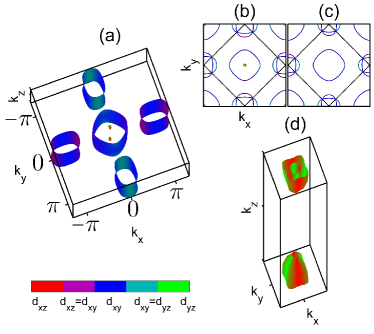
Figure 29: Fermi surface of LiFeAs as deduced from the ARPES experiments: (a) shows the three-dimensional version of the Fermi surface and (b) and (c) refer to the two-dimensional cuts at $|k_{z}|=\pi$ (left) and $k_{z}=0$, respectively. Hole pockets are located a $(0,0)$ and $(\pi,\pi)$ and electron pockets are at $(\pm\pi,0)$ and $(0,\pm\pi)$. In case of $k_{z}=0$, the two tiny hole pockets $h_{1,2}$ vanish just below the FS and only $h_{3}$ and $e_{1,2}$ remain. (d) shows the zoomed region of the first BZ around the $\Gamma-$point of the BZ with tiny $\alpha$ hole pockets.

There is a possibility to obtain a more complex behavior even in systems which contain both hole and electron pockets. One such example is LiFeAs. Its electronic structure contains three hole and two electron pockets, however two $\Gamma-$centered hole pockets have strong 3D dispersion and exist only near $k_{z}=\pi$ (see Fig.29 As a result the FS in the cross-sections at small $k_{z}$ consists of one hole and two electron pockets (hole $\gamma$ pocket and electron $\beta$ pockets), while in the cross-section at $k_{z}$ near $\pi$ the FS consists of three hole pockets and two electron pockets. The orbital content of the FSs for the two $\alpha$ FSs is very different from that for other three FSs. Namely, the two $\Gamma-$centered hole pockets ($\alpha$ pockets) are made chiefly of $d_{xz}$ and $d_{yz}$ orbitals. The other three FSs are made primarily of $d_{xy}$ orbital, with rather small admixture of $d_{xz}$ and $d_{yz}$ orbitals (Refs.peter_lifeas ; ilya_lifeas . These features indicate that the low-energy electronic structure of LiFeAs consists of two very different subsets. One is made out of quasi-2D $\gamma$ and $\beta$ pockets with primarily $d_{xy}$ orbital content, and the other is made out of $\alpha$ pockets, which are highly anisotropic along $k_{z}$ and are made primarily out of $d_{xz}$ and $d_{yz}$ orbitals.

s-wave	$U_{h_{1}h_{1}}$	$U_{h_{2}h_{2}}$	$U_{h_{3}h_{3}}$	$U_{h_{1}h_{2}}$	$U_{h_{1}h_{3}}$	$U_{h_{2}h_{3}}$	$U_{h_{1}e}$	$\alpha_{h_{1}e}$	$U_{h_{2}e}$	$\alpha_{h_{2}e}$	$U_{h_{3}e}$	$\alpha_{h_{3}e}$	$U_{ee}$	$\alpha_{ee}$	$\beta_{ee}$
$J=0.0U$	0.92	0.99	1.21	0.95	0.29	0.23	0.28	-0.34	0.22	-0.49	1.20	-0.12	1.20	-0.12	0.03
$J=0.1U$	0.99	1.09	1.14	1.03	0.16	0.10	0.15	-0.85	0.08	-1.65	1.14	-0.13	1.14	-0.13	0.04
$J=0.3U$	1.14	1.28	1.02	1.20	-0.09	-0.15	-0.12	1.58	-0.18	1.10	1.02	-0.16	1.03	-0.17	0.05

Table 4: LAHA projected interactions in the $s-$wave channel for k${}_{z}=\pi$. The energies are in units of $U$.

s-wave	$U_{h_{3}h_{3}}$	$U_{h_{3}e}$	$\alpha_{h_{3}e}$	$U_{ee}$	$\alpha_{ee}$	$\beta_{ee}$
$J=0.0U$	1.53	1.36	-0.14	1.22	-0.13	0.04
$J=0.1U$	1.48	1.30	-0.16	1.16	-0.14	0.04
$J=0.3U$	1.40	1.19	-0.20	1.04	-0.18	0.06

Table 5: LAHA projected interactions in the $s-$wave channel for k${}_{z}=0$. The energies are in units of $U$.

The results ilya_lifeas for the interactions in $s-$wave channels within LAHA are shown in Tables IV and V. For the model described by Eq. (78) with $U^{\prime}=U-2J$ and $J^{\prime}=J$, we clearly see that the two subsets are nearly separated for all $J/U$. This near-separation opens up a novel possibility for the structure of $s^{+-}$ gap. Namely, superconducting gaps consistent with the structure of interactions in Table IV are

$$\begin{split}\Delta_{h_{1}}(\phi)&=\Delta_{h_{1}}\\ \Delta_{h_{2}}(\phi)&=\Delta_{h_{2}}\\ \Delta_{h_{3}}(\phi)&=\Delta_{h_{3}}\\ \Delta_{e_{1}}(\theta)&=\Delta_{e}+\bar{\Delta}_{e}\cos{2\theta}\\ \Delta_{e_{2}}(\theta)&=\Delta_{e}-\bar{\Delta}_{e}\cos{2\theta}\\ \end{split}$$ (80)

In a "conventional" $s^{+-}$ gap structure, the gaps on the three hole pockets are of the same sign. Here, superconductivity within the subset of the two $\alpha$ pockets is primary due to inter-pocket repulsion between fermions near these pockets. When this repulsion exceeds inter-pocket repulsion, it gives rise to sign-changing $s^{+-}$ superconductivity between these two pockets. In Fig. 30 I show the gap structure obtained for the parameters from Table IV and how it evolves when I artificially increase the interaction between $\alpha$ and $\beta$ pockets. When inter-subset interaction is strong, I obtain a conventional $s^{+-}$ superconductivity, with the same sign of the gap on all three hole pockets peter_lifeas . However, for small/moderate coupling between the $\alpha$ and $\beta-\gamma$ subsets, we see from Fig. 30 that the gaps on the two $\alpha$ pockets are of opposite sign.

Another novel structure of an $s-$wave gap (termed as "orbital antiphase state") has been suggested in Ref. gabi_lifeas . In this state, superconducting gap has the same sign on the two $\alpha$ pockets but changes sign between $\alpha$ pockets and $\gamma$ pocket. Such a state occurs if the coupling between the two subsets is strong and predominantly involves $\alpha-\gamma$ interaction.

VII.5 Superconductivity which breaks time-reversal symmetry

Several groups argued recently that multi-orbital character of FeSCs is an ideal playground to search for a truly novel spin-singlet superconductivity which breaks time-reversal symmetry (TRS). Spin-triplet superconductivity with broken time-reversal symmetry ($p_{x}\pm ip_{y}$ state) has likely been found in $Sr_{2}RuO_{4}$ Mackenzie , which represents a solid-state analog of superfluid ³He Volovikold ; 3he2 , but the spin-singlet $d+id$ state has not yet been observed experimentally. Such a state was once proposed as a candidate state for high $T_{c}$ cuprate superconductors laughlin , but later gave way to a more-conventional TRS-preserving $d-$wave state. A TRS breaking $d+id$ superconductivity has been recently predicted for fermions on a hexagonal lattice (e.g., graphene) near van-Hove doping rahul ; ronny_gr .

For FeSCs, one proposal is to explore the region where $s-$wave and $d-$wave pairing channels are competitive in strength, and there is a transition from one pairing symmetry to the other, as one varies the parameters. In the intermediate regime, the system very likely falls into an intermediate $s+id$ state, with a broken TRS khodas ; ronny_review ; s+id .

There is an even more exotic possibility to get a broken TRS state in an s-wave superconductor zlatko_1 ; maiti_trs ; lara ; egor . Consider as an example a system at extreme hole doping, like Ba_1-xK_xFe₂As₂ at $x\approx 1$ and assume that the superconducting order is $s-$wave, with the sign change of the gap between the two $\Gamma-$centered hole pockets. Once hole doping gets smaller and electron pockets appear, the system eventually develops a "conventional" $s^{+-}$ superconductivity in which the gaps on the two $\Gamma-$centered hole pockets have the same sign. According to theory maiti_trs , the system evolution with decreasing $x$ from a novel to a conventional $s^{+-}$ order may go through an intermediate state in which the relative phase $\phi$ between the gaps on the $\Gamma$-centered hole pockets gradually evolves from $\phi=\pm\pi$ in the novel s-wave state to $\phi=0$ in a conventional $s^{+-}$ state (Fig. 31). In between, the system selects either $\phi$ or $-\phi$, which are related by time-reversal transformation, i.e. it breaks time-reversal symmetry (an $s\pm is$ state).

An intermediate state with broken time-reversal symmetry is also expected in Ba_1-xK_xFe₂As₂ at $x\leq 1$ if the superconducting state in KFe₂As₂ is $d-$wave. In this situation, the system must transform from a $d-$wave at $x=1$ to an $s$-wave at a smaller $x$, and, like I just said, this normally involves an intermediate $s\pm id$ phase. Another recent proposal for TRS broken superconducting state in FeSCs is $s+it$ superconductivity in the co-existence phase with SDW (see Ref. [e_1, ]).

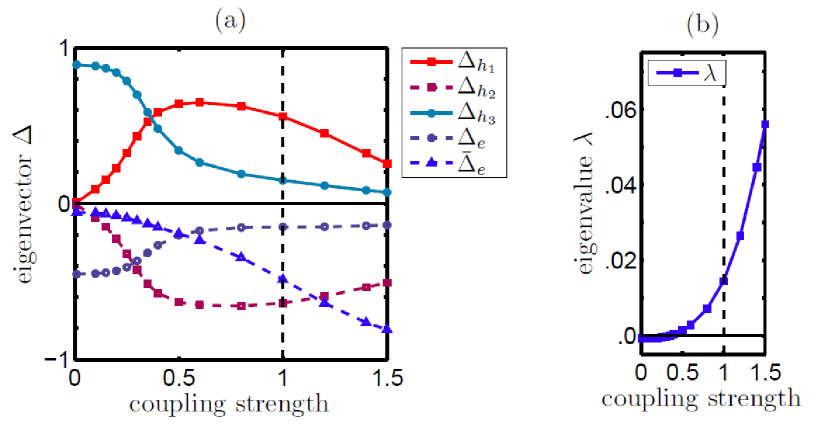
Figure 30: Evolution of the gaps (a) and the largest eigenvalue (b) for the $s-$wave solution, with the coupling between the subset A (the two hole $\alpha$-pockets) and the subset B (the outer hole $\gamma$-pocket and the two electron $\beta$-pockets). From Ref. [ilya_lifeas, ]

VIII Experimental situation on superconductivity in FeSCs

As of today, there is no “smoking gun” experiment which would carry the same weight as phase-sensitive measurements of $d_{x^{2}-y^{2}}$ gap symmetry in the cuprates  [d-wave, ]. Still, there is enough experimental data to minimize the number of possible gap structures.

As we discussed in the previous section, theoretically proposed gap symmetry and structure can be different for weakly/moderately doped systems with hole and electron FSs and for strongly doped systems where FSs of only one type are present. It is then instructive to consider weak/moderate and strong doping separately.

VIII.1 Moderate doping, gap symmetry

The candidates are s-wave (either $s^{\pm}$ or $s^{++}$) or $d_{x^{2}-y^{2}}$ gap. The two behave very differently along the hole FSs centered at $(0,0)$ – s-wave gap is nodeless with $\cos 4\phi$ variations, while d-wave gap has nodes along $k_{x}=\pm k_{y}$. ARPES measurements, both from synchrotron  [Evtush, ; 122hole_ARPES, ; ARPES_1111, ; 122electron_ARPES, ] and using laser light  [laser_arpes, ], show quite convincingly that the gap along hole FSs is nodeless in both hole and electron-doped FeSCs. This unambiguously selects an s-wave. Additional evidence in support of s-wave pairing comes from very flat low-T behavior of the penetration depth in the highest $T_{c}$ 1111 FeSCs systems  [martin_09, ].

VIII.2 Moderate doping, $s^{\pm}$ vs $s^{++}$

The distinction between $s^{\pm}$ and $s^{++}$ gaps is a more subtle issue, particularly given that both belong to the same $A_{1g}$ representation and also because in general $A_{1g}$ gap on electron pockets may have strong oscillating component. In general, the gaps on electron and hole FSs have non-equal magnitudes, and the issue whether the gap is $s^{\pm}$ or $s^{++}$ reduces to whether the gap averaged over an electron FS has the same sign or opposite sign than the gap averaged over a hole FS. This is not a fundamental symmetry issue and, moreover, when $\cos 2\phi$ oscillations are strong, one may switch from equal to opposite signs of the averaged gaps by a small change of parameters  [RG_SM, ] or by adding impurities.  [efremov, ] Still, when oscillations are not very strong, whether the eigenfunction has $s^{\pm}$ or $s^{++}$ character is essential because it determines, to a large extent, whether the pairing is driven by spin or by orbital fluctuations (see Sec.VI).

The experimental data most frequently cited in support of $s^{\pm}$ gap is the observation of a magnetic resonance in neutron scattering  [Cruz, ; resonance, ]. If, as many researchers believe, the resonance is a spin exciton, it exists at a momentum $Q$ if the gaps at FS momenta $k_{F}$ and $k_{F}+Q$ are of opposite sign. Experimentally, in most FeSCs the resonance is observed  [Cruz, ; resonance, ] near $Q=(\pi,\pi)$ in the folded BZ, which in this zone is precisely the distance between electron and hole FSs. The excitonic resonance then exists if the gap changes sign between hole and electron pockets and does not exist if the gap doesn’t change sign. A similar reasoning has been used in identifying the the resonance seen in the cuprates with a fingerprint of $d_{x^{2}-y^{2}}$ gap symmetry  [eschrig, ]

The neutron peak is the resonance if it is narrow and is located below twice the gap value. The argument made by the supporters of $s^{++}$ scenario  [jap, ] is that the observed neutron peak is more broad than the resonance seen in the cuprates, and that there is no firm evidence that the peak energy is below $2\Delta$ for the minimum gap. For $s^{++}$ gap structure, there is no resonance, but there is a redistribution of the neutron spectral weight immediately above 2$\Delta$ what gives rise to a local maximum in the magnetic structure factor  [jap, ; kuroki_11, ; eremin_11, ]. Still, the majority of researchers do believe that the observed neutron peak is a resonance, and the fact that it is quite broad is at least partly due to $\cos 2\phi$ gap variations along the electron FSs [eremin_11, ].

Another rather strong evidence in support of $s^{\pm}$ gap is the observed variation of the quasiparticle interference pattern in a magnetic field  [hanaguri, ] although the interpretation of the data has been subject of debates  [debates, ]. It was also argued  [co-existence_Fe, ] that the very presence of the co-existence region between SC and stripe magnetism in FeSCs is a fingerprint of an $s^{\pm}$ gap, because for $s^{++}$ gap a first order transition between a pure magnetic and a pure SC state is a much more likely scenario.

VIII.3 Moderate doping, nodal vs no-nodal $s^{\pm}$ gap

Let’s assume that the pairing is driven by spin fluctuations and the gap has $s^{\pm}$ structure. In 2D scenario, such gap has $\cos 2\phi$ variations along electron FSs, which, according to theory, can be rather strong, particularly in electron-doped FeSCs. Experimental data show that, whether or not the gap is nodeless or has nodes, depends on the material, on the doping, and on whether SC co-exists with SDW order.

VIII.3.1 Hole doping

For hole-doped FeSCs (e.g. for Ba_1-xK_xFe₂As₂) the data indicate that the gap is nodeless, away from the co-existence region. This is consistent with the theory (see Sec. VII). ARPES experiments do not show any angular variation of the gap along both hole and electron FSs  [Evtush, ; 122hole_ARPES, ], but it is not entirely clear whether ARPES can at present distinguish between the gaps on the two electron FSs which in folded zone are both centered at $(\pi,\pi)$. Thermal conductivity data show that $\kappa/T$ tends to zero in the limit of $T=0$, in line with what one should expect for a nodeless SC  [reid_11, ]. Specific heat data also show non-nodal behavior  [heat_hole, ]. The interpretation of the penetration depth data requires more care as the data do show a power-law behavior $\lambda(T)-\lambda(0)\propto T^{a}$ with $a\sim 2$ (Refs.  [122hole_pen_depth, ]). Such a behavior is expected for a SC with point nodes, but it is also expected in a wide range of $T$ for a nodeless $s^{\pm}$ SC in the presence of modest inter-band scattering by non-magnetic impurities  [impurities, ]. Penetration depth measurements on artificially irradiated samples  [kim_10, ] support the idea that the gap is nodeless and power-law $T^{a}$ behavior of $\lambda(T)-\lambda(0)$ is due to impurities.

VIII.3.2 Electron doping

For electron-doped FeSCs, e.g., 122 materials like Ba(Fe_1-xCo_x)₂As₂ or 1111 materials like NdFeAsO_1-xF_x, ARPES shows no-nodal gap along hole FS  [ARPES_1111, ; 122electron_ARPES, ], but there are no data on the gap along each of the two electron FSs. At optimal doping, the data on both thermal conductivity  [thermal_opt, ; hashimoto, ] and penetration depth  [hashimoto, ; pen_opt, ] are consistent with no-nodal gap However, the data for overdoped Ba(Fe_1-xCo_x)₂As₂ indicate that gap nodes may develop: the behavior of $\lambda(T)$ becomes more steep, and $\kappa/T$ now tends to a finite value  [thermal_opt, ], expected for a SC with line nodes. The data also show $\sqrt{H}$ behavior of $\kappa$ in a magnetic field  [thermal_opt, ] expected for a SC with line nodes  [volovik, ], but it was argued that the behavior resembling $\sqrt{H}$ can be obtained even if $s^{\pm}$ gap has no nodes  [bang, ]. There is also clear anisotropy between in-plane conductivity and conductivity along $z$ direction, what was interpreted  [thermal_opt, ] as an indication that the nodes may be located near particular $k_{z}$. Specific heat data in overdoped Ba(Fe_0.9Co_0.1)₂As₂ were also interpreted as evidence for the nodes.  [heat_el_over, ]

The development of the nodes in $s^{\pm}$ gap upon electron doping is in line with the theory. The farther the system moves away from the SDW phase, the weaker is the increase of intra-band electron-hole interaction and hence the stronger is the competition from intra-band repulsion. As I discussed in Sec.III), the gap adjusts to this change by increasing its $\cos 2\phi$ component in order to effectively reduce the effect of the intra-band repulsion in the gap equation.

There is also experimental evidence for $\cos 2\phi$ gap oscillations from the observed oscillations  [wen_10, ] of the field-induced component of the specific heat $C(H,T)$ in superconducting FeTe_1-xSe_x ($x\sim 0.5$). The measured $C(H,T)$ oscillates with the direction of the applied field as $\cos 4\phi$. In theory, such an oscillation is related to the behavior of $\Delta^{2}(\phi)$ (Ref.  [vekhter_10, ]), hence $\cos 2\phi$ gap oscillations in $\Delta$ lead to $\cos 4\phi$ oscillations in $C(H,T)$. The observed field and temperature dependence of the prefactor for $\cos 4\phi$ term are consistent with the idea that the oscillations are caused by $\cos 2\phi$ term in $\Delta$. These data were also interpreted as evidence for no-nodal gap because if $\cos 2\phi$ gap oscillations were strong and the gap had nodes at accidental points, the behavior of $\Delta^{2}$ would be more complex than the observed $a+b\cos 4\phi$.

For LiFeAs, which is undoped but has FS structure similar to electron-doped FeSCs, no-nodal behavior has been observed in ARPES  [LiFeAs_ARPES2, ], specific heat  [LiFeAs_ARPES1_nutron_scat, ], penetration depth  [thermal_pen_LiFeAs, ] and NMR  [buechner, ; ma_10, ] measurements. An $a+b\cos 4\phi$ variation of the gap on the hole $\gamma$ pocket, consistent with $s-$wave superconductivity, has been observed sergei_b , together with $c+d|\cos 2\phi|$ variations of the gap on electron pockets ding_lifeas . The latter is precisely what is expected theoretically for an s-wave superconductor when the hybridization between the two $\beta$ pockets is weak. The gap on the $\alpha$ pocket probably also has angle dependence, but the pocket is too small to detect it in ARPES measurements.

VIII.3.3 Co-existence region with SDW

Taken at a face value, thermal conductivity and penetration depth data indicate that the gap becomes nodal deep in the co-existence regime in both hole-doped and in electron-doped FeSCs. The most striking evidence comes from thermal conductivity  [thermal_opt, ; reid_11, ] – in the co-existence regime $\kappa/T$ tends to a finite value at $T\to 0$ and shows $\sqrt{H}$ behavior, both typical for a SC with line nodes. From theory perspective, the gap remains nodeless near the onset of co-existence with SDW if it was nodeless outside f the co-existence phase parker , however, deep in the co-existence phase angular variation of the gap increase due to FS reconstruction (Ref. [e_2, ]).

$\begin{array}[]{cc}\includegraphics[width=195.12767pt]{schema}&\includegraphics[width=195.12767pt]{schemb}\end{array}$

Figure 31: Qualitative phase diagram for strongly hole-doped FeSC. I model the doping dependence by varying the ratio of inter-pocket electron-hole and hole-hole interactions $u_{he}/u_{hh}$. The $+-$ state has gaps of opposite signs on the two GCP’s and no gap on electron pockets, the $++$ state is an ordinary $s\pm$ state, in which the gaps have opposite signs on hole and electron pockets. The state with broken TRS is in between the two. The gap structures are pictorially presented inside each region by vectors placed inside the circles. The magnitudes of the vectors represent $|\Delta_{i}|$ and the angles represent the phases. Cases $(a)$ and $(b)$ are for equal and non-equal intra-pocket interactions ($u_{h_{1}}$ and $u_{h_{2}}$) for the two hole pockets, respectively . For ($a$), the state with broken TRS starts right at $T_{c}$ and extends into a finite range at $T=0$. For ($b$), this state splits off from the $T_{c}$ line and is only accessible at lower temperatures, while immediately below $T_{c}$ the $+-$ state gradually evolves into the $++$ state as $u_{he}/u_{hh}$ increases.

VIII.3.4 Isovalent doping

Electron or hole doping is not the only way to change the properties of FeSCs. Another route is to replace one pnictide with the other. The most common replacement is As $\to$ P. P-containing materials include the very first FeSC – LaFeOP, with $T_{c}\leq 5K$ (Ref.  [lafop, ]), the family BaFe₂ As_1-xP_x with the highest $T_{c}$ around 30K (Ref.  [matsuda, ]), and LiFeP  [private, ]. Penetration depth, thermal conductivity, specific heat, and NMR data  [thermal_p, ] in these materials all show the behavior consistent with line nodes. In particular, $\kappa$ scales linearly with $T$ at low $T$ and displays $\sqrt{H}$ behavior in a magnetic field, and $\lambda(T)-\lambda(0)$ is also linear in $T$ down to very low $T$. Laser ARPES data show  [laser_arpes, ] that the gap along FS is nodeless, so the nodes likely are located on electron FSs.

On general grounds, the existence of the nodes on electron FSs is in line with theory predictions particularly as BaFe₂ As_1-xP_x has the same structure of 4 cylindrical FSs as electron-doped FeSCs for which nodes are most likely. It has been argued  [Kuroki, ] that a replacement of As by P changes the hight of a pnictide with respect to Fe plane, what effectively reduces inter-pocket electron-hole interaction, in which case the gap develops nodes to reduce the effect of intra-pocket repulsion. However, this argument is only suggestive, and it is not entirely clear at the moment why all P-based FeSCs have nodes. One way to analyze this semi-quantitatively is to study the correlation between $2\Delta/T_{c}$ on the hole FS and the presence of the nodes on electron FSs. This study shows  [maiti_delta, ] that from this perspective P-based FeSCs are indeed the “best case” for the gap nodes.

Another open issue is the location of the nodes along z- direction. Oscillations of thermal conductivity with the direction of a magnetic field have been measured recently  [vekhter_11, ], and $\cos 4\phi$ component of these oscillations has been interpreted using the modified 2D form of the gap on an electron pocket $\Delta_{e}(k_{z})=\Delta_{0}(1+\alpha(k_{z})\cos 2\phi)$. The best fit to the data yields $\alpha(k_{z})>1$ for some $k_{z}$ and $\alpha(k_{z})<1$ for others, in which case the nodes form patches along $k_{z}$. This gap structure has been reproduced in microscopic calculations khodas_3 , but whether this is the only explanation of the data is unclear.

It is still possible, though, that the nodes are located on a hole FS, near particular $k_{z}$, as some of 3D theories suggest  [3D, ]. Another possibility, which is also not entirely ruled out, is that the system behavior near the surface, probed by ARPES, is not the same as in the bulk. The probability that this is the case is not high, though, because some ARPES data have been obtained using a laser light which probes states located farther from the surface than in conventional synchrotron-based ARPES.

VIII.4 Strongly doped FeSCs

VIII.4.1 Electron doping

Strongly electron doped materials are represented by a family of A_xFe_2-ySe₂ ($A=K,Rb,Cs$)  [exp:AFESE, ; exp:AFESE_ARPES, ] of which K${}_{0}.8$Fe_1.7Se₂ is the most studied material. $T_{c}$ in A_xFe_2-ySe₂ is rather high, almost 40K. ARPES shows  [exp:AFESE_ARPES, ] that only electron FSs are present in A_xFe_2-ySe₂, while hole pockets are at least $60meV$ from the FS, although hole dispersion above $60meV$ is still clearly visible in ARPES. Two electron FSs are at $(0,\pi)$ and $(\pi,0)$, like in other FeSCs, and there is, possibly, another electron FS at $(0,0)$. RPA, LAHA and fRG calculations for these systems predict Maier2011a ; Das2011 ; Das2011 ; Wang2011c ; maiti_11 ; dhl that the gap should have a d-wave symmetry, at least for the case when the FSs are only at $(0,\pi)$ and $(\pi,0)$. A d-wave symmetry in this situation means that the gaps on the two electron FSs behave as $\Delta_{0}(\pm 1+\alpha\cos 2\phi)$, and all calculations yield $\alpha<1$, i.e., no nodes (neglecting 3D effects). One theoretical alternative is $s^{++}$ symmetry by one reason  [kontani_se, ] or the other  [yu_11, ; bernevig, ], another is $s^{+-}$ state between electron pockets mazin_a ; khodas ; khodas_2 . At present, both ARPES exp:AFESE_ARPES and specific heat data Hardy_13 point that the gap is nodeless, at least for most of $k_{z}$ values. Of particular relevance here are ARPES data on a small electron pocket centered at $k_{z}=\pi$ and $k_{x}=k_{y}=0$. These data show kfeas_pi that the gap has no nodes, and, taken at a face value, rule out $d-$wave. At the same time, neutron data clearly show AFESE_neu spin resonance, which, if interpreted as spin exciton eschrig , requires a sign change of the gap. Both ARPRS and neutron data and recent Raman data e_3 are consistent with the novel $s^{+-}$ gap, but more studies are needed to verify whether this state is the right one for A_xFe_2-ySe₂

VIII.4.2 Hole doping

The case of extreme hole doping is represented by KFe₂As₂ ($T_{c}=3K$), which is at the opposite end from parent BaFe₂As₂ in the family of K_xBa_1-xFe₂As₂. According to ARPES  [KFeAs_ARPES_QO, ], this system has no electron pockets. It contains hole pockets at $(0,0)$ and additional hole pockets around $(\pi,\pi)$, but whether the latter play any role for superconductivity is not clear at the moment.

Both thermal conductivity and penetration depth measurements clearly point to nodal behavior [KFeAs_exp_nodal, ]. There is, however, no “smoking gun” symmetry-sensitive measurement, so whether the gap is a d-wave or an $s$-wave with nodes due to strong $\cos 4\phi$ gap component on one of the FSs remains an open issue. Recent study of $T_{c}$ under pressure has found louis_last that $T_{c}$ initially decreases with pressure initially, and then suddenly changes trend above a critical pressure $P_{c}$ and start increasing. This is a strong indication of the near-degeneracy between different pairing states in KFe₂As₂. These states can be $s$ and $d$, or different $s-$wave states. Like I said before, some theorists suggested mixed states, like $s+id$ or $s+is$, which break TRS. Zero-field $\mu$SR measurements so far have not detected spontaneous internal magnetic fields, expected for $s+id$ state sonier . Whether such fields are generated for $s+is$ state is less clear. This is an active field of research and I refrain from discussing it in more detail.

VIII.4.3 FeTe_1-xSe_x

There has been high interest recently in the properties of Fe-chalcogenide FeTe_1-xSe_x. The parent compound FeTe_x is a SDW metal, but with high magnetic moment and magnetic order different from that in Fe-pnictides (see dukatman for details). Superconductivity emerges around $x=0.5$, and magnetic fluctuations and FS-geometry at these $x$ do not differ substantially from Fe-pnictides, and it is reasonable to expect that magnetic fluctuations may mediate $s^{+-}$ supeconductivity. This, however, has not been studied in detail yet. On the other end, at $x=1$, the system behavior is quite unusual – the structural transition sets in at around $80K$ (see dresden ), well before magnetic fluctuations develop. Structural order increases as $T$ decreases, but changes trend below superconducting $T_{c}\sim 9$, what clearly shows that structural order competes with superconductivity. The existence of structural transition without strong magnetic fluctuations fueled speculations that structural order in FeSe may reflect spontaneous orbital order, i.e., orbital fluctuations are "in the driver’s seat". If this is the case, one should expect $s^{++}$ superconductivity in this material. Experimental studies in the superconducting state of FeTe_1-xSe_x are called for to resolve this issue. There is also an interesting and highly unusual system behavior under pressure – structural transition temperature goes down and magnetic fluctuations rapidly develop pressure .

A highly unusual behavior has been detected in thin films of FeSe. ARPES measurements detected only electron pockets arpes_filmsfese , like in K_xFe_2-ySe₂. Like in K_xFe_2-ySe₂, $T_{c}$ is rather high, $T_{c}\sim 60K$ (even higher $T_{c}$ have been reported tcspecul ). Whether FeSe (and, more generally, FeTe_1-xSe_x for $x\geq 0.5$) falls into the same category as Fe-pnictides remains to be seen.

VIII.5 Summary

Overall, the agreement between itinerant theory and experiment with respect to the type of SDW order, the interplay between the nematic order and magnetism (e.g., the normal state phase diagram as a function of doping) and the symmetry and structure of the superconducting gap is reasonably good. With respect to superconductivity, itinerant approach predicts that the gap is $s^{+-}$ in most systems, with angular variation, chiefly on electron pockets, and with accidental nodes in some systems. A more complex gap structure emerges in systems with strong hole or strong electron doping.

IX Conclusion

he analysis of the normal state behavior and superconductivity in FeSCs is a fascinating subject because of multi-orbital/multi-band nature of these materials. This review is an attempt to present a coherent picture of itinerant scenario for FeSCs. I discussed the SDW magnetism, which in most FeSCs corresponds to stripe order, the pre-emptive nematic phase, and the origin of superconductivity and the symmetry and structure of the superconducting gap in different classes of FeSCs and at different doping levels. It is safe to say that there is no major disagreement between theory predictions within the itinerant scenario and the experiments. This by no means implies that FeSCs fall into a class of "weakly coupled Fermi liquids". There are numerous indications that the coupling is strong and is not that much different from that in the cuprates, where, we know, Mott state does develop near half-filling. Nevertheless, most of parent compounds of FeSCs are metals, and, in my view, that low-energy physics of FeSCs is adequately captured within a moderate coupling itinerant scenario. Up to what temperature/energy one can extent the itinerant approach is another question. This scale varies from material to material, but, still, is larger than the scales associated with superconducting $T_{c}$ and is likely larger that SDW transition temperature $T_{sdw}$ and the temperature $T_{n}$ associated with the development of a nematic order. The physics at higher temperature/energies is outside the validity of the itinerant approach.

References

- (1) Y. Kamihara, T. Watanabe, M. Hirano, H. Hosono, J. Am. Chem. Soc. 130, 3296(2008).
- (2) X. H. Chen, T. Wu, G. Wu, R. H. Liu, H. Chen, D. F. Fang, Nature 453, 761(2008).
- (3) G. F. Chen, Z. Li, D. Wu, G. Li, W. Z. Hu et al Phys. Rev. Lett. 100, 247002 (2008).
- (4) Z.-A. Ren, G.-C. Che, X.-L. Dong, J. Yang, W. Lu et al Europhys. Lett. 83, 17002(2008)
- (5) M. Rotter, M. Tegel, D. Johrendt, Phys. Rev. Lett. 101, 107006 (2008)
- (6) K. Sasmal, B. Lv, B. Lorenz, A. M. Guloy, F. Chen, Y.-Y. Xue, and C.-W. Chu, Phys. Rev. Lett. 101, 107007 (2008),
- (7) N. Ni, A. Thaler, J. Q. Yan, A. Kracher, E. Colombier, S. L. Bud’ko, P. C. Canfield, Phys. Rev. B 82, 024519 (2010).
- (8) X.C.Wang, Q.Q. Liu, Y.X. Lv, W.B. Gao, L.X.Yang, R.C.Yu, F.Y.Li, and C.Q. Jin, arXiv:0806.4688v3; S. V. Borisenko, V. B. Zabolotnyy, D. V. Evtushinsky, T. K. Kim, I. V. Morozov et al Phys. Rev. Lett. 105, 067002 (2010).
- (9) Y. Mizuguchi, F. Tomioka, S. Tsuda, T. Yamaguchi, and Y. Takano, Appl. Phys. Lett. 93, 152505 (2008), F. C. Hsu et al., Proc. Natl. Acad. Sci. U.S.A. 105, 14 262 (2008), M. H. Fang, H. M. Pham, B. Qian, T. J. Liu, E. K. Vehstedt, Y. Liu, L. Spinu, and Z. Q. Mao, Phys. Rev. B 78, 224503 (2008), G. F. Chen, Z. G. Chen, J. Dong, W. Z. Hu, G. Li, X. D. Zhang, P. Zheng, J. L. Luo, and N. L. Wang, Phys. Rev. B 79, 140509(R) (2009).
- (10) J. Guo, S. Jin, G. Wang, S. Wang, K. Zhu, T. Zhou, M. He, and X. Chen, Phys. Rev. B 82, 180520(R) (2010). See Y. Liu, Z. C. Li, W. P. Liu, G. Friemel, D. S. Inosov, R. E. Dinnebier, Z. J. Li, and C. T. Lin, Supercond. Sci. Technol. 25, 075001 (2012).
- (11) T. Qian, X.-P. Wang, W.-C. Jin, P. Zhang, P. Richard, G. Xu, X. Dai, Z. Fang, J.-G. Guo, X.-L. Chen, H. Ding, Phys. Rev. Lett. 106, 187001 (2011).
- (12) Y. Nakai, T. Iye, S. Kitagawa, K. Ishida, H. Ikeda, S. Kasahara, H. Shishido, T. Shibauchi, Y. Matsuda, T. Terashima, Phys. Rev. Lett. 105, 107003 (2010).
- (13) see e.g., S. Kasahara, K. Hashimoto, H. Ikeda, T. Terashima, Y. Matsuda, T. Shibauchi, Phys. Rev. B 85, 060503(R) (2012).
- (14) Y. Kamihara, T. Watanabe, M. Hirano, and H. Hosono, J. Am. Chem. Soc. 128, 10012 (2006).
- (15) For the latest results on magnetic measaurements, see D. S. Inosov, J. T. Park, P. Bourges, D. L. Sun, Y. Sidis, A. Schneidewind, K. Hradil, D. Haug, C. T. Lin, B. Keimer, and V. Hinkov, Nature Physics 6, 178-181 (2010) and references therein.
- (16) see e.g., E. Abrahams and Q. Si, J. Phys.: Condens. Matter 23, 223201 (2011); C. Weber and F. Mila, arXiv:1207.0095.
- (17) Ming Yi, Donghui Lu, Rong Yu, Scott Riggs, Jiun-Haw Chu, Bing Lv, Zhongkai Liu, Minghui Lu, Yongtao Cui, Makoto Hashimoto, Sung-Kwan Mo, Zahid Hussain, Ching-Wu Chu, Ian Fisher, Qimiao Si, Zhi-Xun Shen, PRL 110, 067003 (2013)
- (18) M.J. Calderón, L. de’ Medici, B. Valenzuela, E. Bascones, Phys. Rev. B 90, 115128 (2014); L. de’ Medici, G. Giovannetti, M. Capone, Phys. Rev. Lett. 112, 177001 (2014).
- (19) D.C. Johnston, Adv. Phys., 59, 803 (2010).
- (20) see e.g., I. A. Zaliznyak, et al, Z. J. Xu, J. S. Wen, J. M. Tranquada, G. D. Gu, V. Solovyov, V. N. Glazkov, A. I. Zheludev, V. O. Garlea, and M. B. Stone, Phys. Rev. B 85, 085105 (2012) and references therein.
- (21) J-P Paglione and R.L. Greene, Nature Phys. 6, 645 (2010).
- (22) I.I. Mazin, Nature 464, 183 (2010).
- (23) H.H. Wen and S. Li, Annu. Rev. Condens. Matter Phys., 2, 121 (2011).
- (24) S. Graser, T. A. Maier, P. J. Hirshfeld, D. J. Scalapino, New J. Phys. 11, 025016 (2009).
- (25) A. F. Kemper, T. A. Maier, S. Graser, H.-P. Cheng, P. J. Hirschfeld, and D. J. Scalapino, New J. Phys. 12, 073030 (2010).
- (26) K. Kuroki, H. Usui, S. Onari, R. Arita, and H. Aoki, Phys. Rev. B 79, 224511 (2009).
- (27) A. V. Chubukov Physica C 469, 640(2009).
- (28) I.I. Mazin and J. Schmalian, Physica C, 469, 614 (2009).
- (29) D.N. Basov and A.V. Chubukov, Nature Physics 7, 241 (2011).
- (30) P.J. Hirschfeld, M.M. Korshunov, and I.I. Mazin, Reports on Progress in Physics 74, 124508 (2011).
- (31) A.V, Chubukov, Annual Review of Condensed Matter Physics 3, 57 (2012).
- (32) S. Maiti and A V. Chubukov, arXiv:1305.4609, in "Proceedings of the XVII Training Course in the physics of Strongly Correlated Systems", Vietri sul Mare (Salerno), Italy.
- (33) T. Yildirim, Phys. Rev. Lett. 101, 057010 (2008).
- (34) F. Ma, Z.-Y. Lu, and T. Xiang, Phys. Rev. B 78, 224517 (2008).
- (35) Avci, S. et al. Nature Comm. 5, 3845 (2014).
- (36) X. Wang and R. M. Fernandes, Phys. Rev. B 89, 144502 (2014).
- (37) I. R. Fisher, L. Degiorgi, and Z. X. Shen, Rep. Prog. Phys. 74, 124506 (2011).
- (38) J.-H. Chu, J. G. Analytis, K. De Greve, P. L. McMahon, Z. Islam, Y. Yamamoto, and I. R. Fisher, Science 329, 824 (2010).
- (39) M. A. Tanatar, E. C. Blomberg, A. Kreyssig, M. G. Kim, N. Ni, A. Thaler, S. L. Bud’ko, P. C. Canfield, A. I. Goldman, I. I. Mazin, and R. Prozorov, Phys. Rev. B 81, 184508 (2010).
- (40) A. Dusza, A. Lucarelli, F. Pfuner, J.-H. Chu, I. R. Fisher, and L. Degiorgi, EPL 93, 37002 (2011); A. Lucarelli, A. Dusza, A. Sanna, S. Massidda, J.-H. Chu, I.R. Fisher, and L. Degiorgi, New J. Phys. 14, 023020 (2012).
- (41) M. Nakajima, T. Liang, S. Ishida, Y. Tomioka, K. Kihou, C. H. Lee, A. Iyo, H. Eisaki, T. Kakeshita, T. Ito, and S. Uchida, PNAS 108, 12238 (2011).
- (42) T.-M. Chuang, M. P. Allan, J. Lee, Y. Xie, N. Ni, S. L. Bud’ko, G. S. Boebinger, P. C. Canfield, and J. C. Davis, Science 327, 181 (2010).
- (43) M. Yi, D. Lu, J.-H Chu, J. G. Analytis, A. P. Sorini, A. F. Kemper, B. Moritz, S.-K. Mo, R. G. Moore, M. Hashimoto, W.-S. Lee, Z. Hussain, T. P. Devereaux, I. R. Fisher, and Z.-X. Shen, PNAS 108, 6878 (2011).
- (44) S. Kasahara, H.J. Shi, K. Hashimoto, S. Tonegawa, Y. Mizukami, T. Shibauchi, K. Sugimoto, T. Fukuda, T. Terashima, Andriy H. Nevidomskyy, Y. Matsuda Nature 486, 382-385 (2012).
- (45) C.-L. Song, Y.-L. Wang, P. Cheng, Y.-P. Jiang, W. Li, T. Zhang, Z. Li, K. He, L. Wang, J.-F. Jia, H.-H. Hung, C. Wu, X. Ma, X. Chen, and Q.-K. Xue, Science 332, 1410 (2011).
- (46) R. M. Fernandes, D. K. Pratt, W. Tian, J. Zarestky, A. Kreyssig, S. Nandi, M. G. Kim, A. Thaler, N. Ni, P. C. Canfield, R. J. McQueeney, J. Schmalian, and A. I. Goldman, Phys. Rev. B 81, 140501(R) (2010).
- (47) S. Nandi, M. G. Kim, A. Kreyssig, R. M. Fernandes, D. K. Pratt, A. Thaler, N. Ni, S. L. Bud’ko, P. C. Canfield, J. Schmalian, R. J. McQueeney, and A. I. Goldman, Phys. Rev. Lett. 104, 057006 (2010).
- (48) M. G. Kim, R. M. Fernandes, A. Kreyssig, J. W. Kim, A. Thaler, S. L. Bud’ko, P. C. Canfield, R. J. McQueeney, J. Schmalian, and A. I. Goldman, Phys. Rev. B 83, 134522 (2011).
- (49) C. R. Rotundu and R. J. Birgeneau, arXiv:1106.5761
- (50) K. Proke¨, S. Mat’a¨, L. Harnagea, S. Singh, S. Wurmehl, D. N. Argyriou, and B. Büchner, Phys. Rev. B 83, 104414 (2011).
- (51) J. Bardeen, L. Cooper, J. R. Schrieffer, Phys. Rev. 108, 1175-1204 (1957).
- (52) S. L. Bud’ko, G. Lapertot, C. Petrovic, C. E. Cunningham, N. Anderson, and P. C. Canfield, Phys. Rev. Lett. 86, 1877 (2001).
- (53) A.J. Leggett, Rev. Mod. Phys. 47, 331(1975), R. Balian, R. and N. R. Werthamer, Phys. Rev. 131, 1553 (1963). P.W. Anderson, and W.F.Brinkman, Phys. Rev. Lett. 30 , 1108 (1973).
- (54) D. Vollhardt and P. Woelfle, Superfluid phases of Helium 3, Taylor and Francis, London, 1990.
- (55) J. G. Bednorz and K. A. Müller, Zeitschrift für Physik B Condensed Matter, 64, 189 (1986).
- (56) E. M. Lifshitz and L. P. Pitaevski, Statistical Physics, (Pergamon Press, 1980).
- (57) W. Kohn and J. M. Luttinger, Phys. Rev. Letters, 15, 524 (1965).
- (58) see e.g., B. Goss Levi, Physics Today, January 1996, Page 19 and references therein.
- (59) I. I. Mazin, D. J. Singh, M. D. Johannes, and M. H. Du, Phys. Rev. Lett. 101, 057003 (2008).
- (60) K. Kuroki, S. Onari, R. Arita, H. Usui, Y. Tanaka, H. Kontani, and H. Aoki Phys. Rev. Lett. 101, 087004 (2008).
- (61) Seiichiro Onari and Hiroshi Kontani, Phys. Rev. Lett. 103, 177001 (2009).
- (62) W.G. Yin, C. C. Lee, and Wei Ku, Phys. Rev. Lett. 105, 107004 (2010).
- (63) R. Fernandes, A.V. Chubukov, I. Eremin, J. Knolle, and J. Schmalian, Phys. Rev. B 85, 024534 (2012).
- (64) R.M. Fernandes, A.V. Chubukov, and J. Schmalian, Nature Phys. 10, 97 (2014).
- (65) P. A. Lee and X.-G. Wen, Phys. Rev. B 78, 144517 (2008).
- (66) Y. Ota, K. Okazaki, Y. Kotani, T. Shimojima, W. Malaeb, S. Watanabe, C. -T. Chen, K. Kihou, C. H. Lee, A. Iyo, H. Eisaki, T. Saito, H. Fukazawa, Y. Kohori, S. Shin, Phys. Rev. B 89, 081103 (2014) and references therein.
- (67) T. Hanaguri, S. Niitaka, K. Kuroki, and H. Takagi Science 328, 474 (2010).
- (68) H. Ding, P. Richard, K. Nakayama, K. Sugawara, T. Arakane et al Europhys. Lett., 83, 47001 (2008).
- (69) T. Y. Chen, Z. Tesanovic, R. H. Liu, X. H. Chen, and C. L. Chien, Nature, 453, 1224 (2008).
- (70) A. D. Christianson, E. A. Goremychkin, R. Osborn, S. Rosenkranz, M. D. Lumsden, C. D. Malliakas, I. S. Todorov, H. Claus, D. Y. Chung, M. G. Kanatzidis, R. I. Bewley, and T. Guidi, Nature, 456, 930 (2008).
- (71) L. Malone, J. D. Fletcher, A. Serafin, A. Carrington, N. D. Zhigadlo, Z. Bukowski, S. Katrych, and J. Karpinski, Phys. Rev. B 79, 140501(R) (2009).
- (72) S. Kasahara et al, Phys. Rev. B 81, 184519, (2010).
- (73) J. D. Fletcher, A. Serafin, L. Malone, J. Analytis, J.-H. Chu, A. S. Erickson, I. R. Fisher, and A. Carrington, Phys. Rev. Lett. 102, 147001 (2009).
- (74) R. T. Gordon, N. Ni, C. Martin, M. A. Tanatar, M. D. Vannette, H. Kim et al Phys. Rev. Lett., 102, 127004 (2009).
- (75) C. Martin, R. T. Gordon, M. A. Tanatar, H. Kim, N. Ni, S. L. Bud’ko et al Phys. Rev. B 80, 020501(R) (2009).
- (76) L. Luan, O. M. Auslaender, T. M. Lippman, C. W. Hicks, B. Kalisky et al Phys. Rev. B 81, 100501(R) (2010).
- (77) see e.g., J. Guo, S. Jin, G.Wang, S.Wang, K.Zhu, et al. Phys. Rev. B 82, 180520 (2010).
- (78) K. Okazaki et al., Science 337, 1314 (2012).
- (79) J.-Ph. Reid, M. A. Tanatar, A. Juneau-Fecteau, R. T. Gordon, S. Rene de Cotret, N. Doiron-Leyraud, T. Saito, H. Fukazawa, Y. Kohori, K. Kihou, C. H. Lee, A. Iyo, H. Eisaki, R. Prozorov, and L. Taillefer, Phys. Rev. Lett. 109, 087001 (2012).
- (80) D. Watanabe, T. Yamashita, Y. Kawamoto, S. Kurata, Y. Mizukami, T. Ohta, S. Kasahara, M. Yamashita, T. Saito, H. Fukazawa, Y. Kohori, S. Ishida, K. Kihou, C. H. Lee, A. Iyo, H. Eisaki, A. B. Vorontsov, T. Shibauchi, and Y. Matsuda, Phys. Rev. B 89, 115112 (2014).
- (81) G. Friemel et al, Phys. Rev. B 85, 140511 (2012).
- (82) A. Kreisel, Y. Wang, T. A. Maier, P. J. Hirschfeld, D. J. Scalapino, Phys. Rev. B 88, 094522 (2013).
- (83) S. Pandey, A. V. Chubukov, and M. Khodas Phys. Rev. B 88, 224505 (2013).
- (84) S. Maiti, M. M. Korshunov, T. A. Maier, P. J. Hirschfeld, and A. V. Chubukov, Phys. Rev. Lett. 107, 147002 (2011); S. Maiti, M. M. Korshunov, T. A. Maier, P. J. Hirschfeld, and A. V. Chubukov, Phys. Rev. B. 84, 224505 (2011).
- (85) M. Yi, D. H. Lu, J. G. Analytis, J.-H. Chu, S.-K. Mo et al Phys. Rev. B 80, 024515 (2009)
- (86) T. Sato, K. Nakayama, Y. Sekiba, P. Richard, Y.-M. Xu et al Phys. Rev. Lett. 103, 047002 (2009); T. Terashima et al., J. Phys. Soc. Japan 79, 053702 (2010).
- (87) S. E. Sebastian, J. Gillett, N. Harrison, P. H. C. Lau, C. H. Mielke, and G. G. Lonzarich, J. Phys.: Condens. Matter 20 422203(2008).
- (88) D. V. Evtushinsky, D. S. Inosov, V. B. Zabolotnyy, M. S. Viazovska, R. Khasanov et al New J. Phys. 11, 055069 (2009);
- (89) J. K. Dong, S. Y. Zhou, T. Y. Guan, H. Zhang, Y. F. Dai et al Phys. Rev. Lett. 104, 087005 (2010); K. Hashimoto, A. Serafin, S. Tonegawa, R. Katsumata, R. Okazaki et al., Phys. Rev. B 82, 014526 (2010).
- (90) P. M. R. Brydon, M. Daghofer, C. Timm, J. van den Brink, Phys. Rev. B 83, 060501 (2011).
- (91) D.J. Singh and M.-H. Du, Phys. Rev. Lett. 100, 237003 (2008); M.J. Calderon, B. Valenzuela, and E. Bascones, Phys. Rev. B 80, 094531 (2009).
- (92) L. Boeri, O. V. Dolgov, and A. A. Golubov, Phys. Rev. Lett. 101, 026403 (2008)
- (93) I.I. Mazin, arXiv:1102.3655 (unpublished).
- (94) S. Graser, A. F. Kemper, T. A. Maier, H.-P. Cheng, P. J. Hirschfeld, and D. J. Scalapino, Phys. Rev. B 81, 214503 (2010).
- (95) S. Onari, H. Kontani, M. Sato, Phys. Rev. B. 81, 060504(R) (2010), H. Kontani, S. Onari, Phys. Rev. Lett. 104, 157001 (2010), T. Saito, S. Onari, H. Kontani, Phys. Rev. B 82, 144510 (2010).
- (96) A.V. Chubukov, M.G. Vavilov, A.B. Vorontsov Phys. Rev. B 80, 140515(R) (2009).
- (97) V. Cvetkovic and O. Vafek, Phys. Rev. B 88, 134510 (2013).
- (98) R. Thomale, C. Platt, J. Hu, C. Honerkamp, and B. Andrei Bernevig Phys. Rev. B 80, 180505(R) (2009),
- (99) K. Suzuki, H. Usui, and K. Kuroki, Phys. Rev. B 84, 144514 (2011). R. Thomale, C. Platt, W. Hanke, J-P Hu, and B. Andrei Bernevig, Phys. Rev. Lett. 107, 117001 (2011). T. A. Maier, S. Graser, P. J. Hirschfeld, and D. J. Scalapino, Phys. Rev. B 83, 100515(R) (2011).
- (100) see e.g., D.J. Scalapino, Rev. Mod. Phys. 84, 1383 (2012)
- (101) S. Maiti and A.V. Chubukov, "Superconductivity from a repilsive interaction" in "Novel Superconductors", Chapter 15, Bennemann and Ketterson eds., Oxford Press 2014.
- (102) H. Meier, C. Pépin, K. B. Efetov, Phys. Rev. B 84, 205131 (2011).
- (103) D. F. Mross, J. McGreevy, H. Liu, T. Senthil Phys. Rev. B 82, 045121 (2010).
- (104) D.L. Maslov and A.V. Chubukov, Phys Rev. B. 81, 045110 (2010).
- (105) M. Dzero and L. P. Gor’kov Phys. Rev. B 69, 092501 (2004).
- (106) H. Zhai, F. Wang, and D.-H. Lee, Phys. Rev. B 80, 064517 (2009).
- (107) R. Thomale, C. Platt, J. Hu, C. Honerkamp, and B. A. Bernevig Phys. Rev. B 80, 180505(R) (2009).
- (108) S. Maiti and A.V. Chubukov, Phys. Rev. B 82, 214515(2010).
- (109) R. Shankar, Rev. Mod. Phys. 66, 129 (1994); W. Metzner, C. Castellani, and C. Di Castro, Adv. Phys. 47, 317 (1998); M. Salmhofer, Commun. Math. Phys. 194, 249 (1998).
- (110) V.S. de Carvalho, H. Freire, Europhys. Lett. 96, 17006 (2011).
- (111) N. Furukawa, T. M. Rice, and M. Salmhofer, Phys. Rev. Lett. 81, 3195 (1998); M. Salmhofer et al, Prog. Theor. Phys. 112, 943 (2004); K. Le Hur and T. M. Rice, Annals of Physics 324 (2009) 1452
- (112) A. V. Chubukov, D. Efremov, and I. Eremin, Phys. Rev. B 78, 134512 (2008).
- (113) Nandkishore, L. Levitov, A. Chubukov, Nature Physics 8, 158-163 (2012).
- (114) Daniel Podolsky, Hae-Young Kee, and Yong Baek Kim, Europhysics Letters 88, 17004 (2009).
- (115) M.A. Metlitski and S. Sachdev, Phys. Rev. B. 82, 075128 (2010).
- (116) K. B. Efetov, H. Meier, C. Pépin, Nat. Phys. 9, 442 (2013).
- (117) A.V. Chubukov, Physics 3, 54 (2010).
- (118) M. G. Vavilov, A. V. Chubukov, A. B. Vorontsov, Supercond. Sci. Technol. 23, 054011 (2010).
- (119) R. M. Fernandes, J. Schmalian, Phys. Rev. B 82, 014521 (2010).
- (120) Eremin, I. and Chubukov, A. V. Phys. Rev. B 81, 024511 (2010).
- (121) A. B. Vorontsov, M. G. Vavilov, and A. V. Chubukov, Phys. Rev. B 81, 174538 (2010).
- (122) V. Cvetkovic and Z. Tesanovic, Phys. Rev. B 80, 024512 (2009).
- (123) V. Barzykin and L. P. Gor’kov, JETP Lett. 88, 131 (2008).
- (124) P. M. R. Brydon and C. Timm, Phys. Rev. B 79, 180504(R) (2009); B. Zocher, C. Timm, and P. M. R. Brydon, arXiv:1106.5315
- (125) K. Kuroki, S. Onari, R. Arita, H. Usui, Y. Tanaka, H. Kontani, and H. Aoki, Phys. Rev. Lett. 101, 087004 (2008).
- (126) F. Wang, H. Zhai, Y. Ran, A. Vishwanath, and D.-H. Lee, Phys. Rev. Lett. 102, 047005 (2009).
- (127) C. Platt, C. Honerkamp, and W. Hanke, New J. Phys. 11, 055058 (2009).
- (128) A. B. Vorontsov, M. G. Vavilov, and A. V. Chubukov, Phys. Rev. B 79, 060508(R) (2009).
- (129) J. Knolle, I. Eremin, A.V. Chubukov, and R. Moessner, Phys. Rev. B 81, 140506(R) (2010).
- (130) P. M. R. Brydon, J. Schmiedt, and C. Timm, arXiv:1109.2071
- (131) C. Cao, P.J. Hirschfeld, H.-P. Cheng, Phys. Rev. B 77, 220506(R) (2008).
- (132) R. Yu, P. Goswami, Q. Si, P. Nikolic, and J-X Zhu, arXiv:1103.3259.
- (133) M. Khodas and A. V. Chubukov Phys. Rev. Lett. 108, 247003 (2012)
- (134) I. I. Mazin, Phys. Rev. B 84, 024529 (2011).
- (135) Jiangping Hu, Phys. Rev. X 3, 031004 (2013) and references therein.
- (136) S. Maiti, M. M. Korshunov, A. V. Chubukov, Phys. Rev. B 85, 014511 (2012)
- (137) Y. Wang, A. Kreisel, V. B. Zabolotnyy, S. V. Borisenko, B. Büchner, T. A. Maier, P. J. Hirschfeld, D. J. Scalapino arXiv:1310.3517.
- (138) F. Ahn et al Phys. Rev. B 89, 144513 (2014).
- (139) Z. P. Yin, K. Haule, and G. Kotliar, arXiv:1311.1188.
- (140) M. Kiesel, Ch. Platt, W. Hanke, D. A. Abanin, and R. Thomale, Phys. Rev. B 86, 020507 (2012).
- (141) see e.g., Ch. Platt, R. Thomale, C. Honerkamp, S-C. Zhang, and W. Hanke Phys. Rev. B 85, 180502 (2012)
- (142) Ch. Platt, W. Hanke, and R. Thomale, arXiv:1310.6191, Advances in Physics (2014).
- (143) V. Stanev, J. Kang, Z. Tesanovic, Phys. Rev. B 78, 184509 (2008); V. Stanev, B. S. Alexandrov, P. Nikolić and Z. Tešanović, arXiv:1006.0447; V. Cvetkovic and Z. Tesanovic, Phys. Rev. B 80, 024512(2009)
- (144) V. Stanev and Z. Tesanovic, Phys. Rev. B 81, 134522 (2010).
- (145) S. Maiti and A. V. Chubukov, Phys. Rev. B 87, 144511 (2013)
- (146) M. Marciani, L. Fanfarillo, C. Castellani, L. Benfatto, arXiv:1306.5545.
- (147) D.F. Agtenberg, V. Barzykin, and L.P. Gorkov, Phys. Rev. B 60, 14868 (1999); L. Fanfarillo, L. Benfatto, S. Caprara, C. Castellani, and M. Grilli, Phys. Rev. B 79, 172508 (2009); T.K. Ng and N. Nagaosa, Europhys. Lett. 87, 17003 (2009); Y. Tanaka and T. Yanagisawa, Solid. State. Comm. 150, 1980 (2010); J. Carlström, J. Garaud, and E. Babaev, Phys. Rev. B 84, 134518 (2011); I. Bobkova and A. Bobkov, Phys. Rev. B 84, 134527 (2011); X. Hu and Z. Wang, Phys. Rev. B 85, 064516 (2011); T. Yanagisawa, Y. Tanaka1, I. Hase, and K. Yamaji, J. Phys. Soc. Jpn. 81 024712 (2012); S.-Z. Lin and X. Hu, Phys. Rev. Lett. 108, 177005 (2012); G. Livanas, A. Aperis, P. Kotetes, G. Varelogiannis, arXiv:1208.2881 (2012); V. Stanev, Phys. Rev. B 85, 174520 (2012).
- (148) Kang, J. and Tesanovic, Z. Phys. Rev. B 83, 020505 (2011).
- (149) T. Saito, S. Onari, and H. Kontani, Phys. Rev. B 83, 140512(R) (2011).
- (150) A. V. Chubukov, M. G. Vavilov, A. B. Vorontsov, Phys. Rev. B 80, 140515(R)(2009)
- (151) Q. Si and E. Abrahams, Phys. Rev. Lett. 101, 076401 (2008).
- (152) R. Thomale, C. Platt, W. Hanke, J-P. Hu, and B. A. Bernevig, arXiv:1101.3593.
- (153) K. Suzuki, H. Usui, and K. Kuroki arXiv:1108.0657.
- (154) K. Nakayama, T. Sato, P. Richard, Y.-M. Xu, T. Kawahara, K. Umezawa, T. Qian, M. Neupane, G. F. Chen, H. Ding, and T. Takahashi, Phys. Rev. B 83, 020501 (2011); Y-M. Xu, Y-B. Huang, X-Y. Cui, E. Razzoli, M. Radovic et al Nature Physics 7, 198-202 (2011).
- (155) T. Kondo, A. F. Santander-Syro, O. Copie, C. Liu, M. E. Tillman, et al Phys. Rev. Lett. 101, 147003 (2008).
- (156) Y. Sekiba, T Sato, K Nakayama, K Terashima, P Richard et al New J. Phys. 11, 025020 (2009); K. Terashima et. al., Proceedings of the National Academy of Sciences of the USA (PNAS) 106, 7330 (2009).
- (157) C. Martin, M. E. Tillman, H. Kim, M. A. Tanatar, S. K. Kim et al Phys. Rev. Lett. 102, 247002 (2009).
- (158) D.V. Efremov, M.M. Korshunov, O.V. Dolgov, A.A. Golubov, and P.J. Hirschfeld, Phys. Rev. B 84, 180512(R) (2011).
- (159) A. D. Christianson, E. A. Goremychkin, R. Osborn, S. Rosenkranz, M. D. Lumsden, et. al., Nature 456, 930 (2008); R. Osborn, J.-P. Castellan, S. Rosenkranz, E. A. Goremychkin, D. Y. Chung, et al, arXiv:1106:0771.
- (160) see e.g. Ar. Abanov, A. V. Chubukov, and J. Schmalian Journal of Electron Spectroscopy and Related Phenomena, 117, 129 (2001); M. Eschrig, Adv. Phys. 55, 47 (2006), and references therein.
- (161) Y. Nagai and K. Kuroki, arXiv:1103.0586; T.A. Maier, S. Graser, P.J. Hirschfeld, D.J. Scalapino, Phys. Rev. B 83, 220505(R) (2011).
- (162) S. Maiti, J. Knolle, I. Eremin, and A.V. Chubukov, arXiv:1108:0266
- (163) I.I. Mazin amd D.J. Singh, arXiv 1007.0047; T. Hanaguri, S. Niitaka, K. Kuroki, and H. Takagi, arXiv:1007.0307.
- (164) R. M. Fernandes, D. K. Pratt, W. Tian, J. Zarestky, A. Kreyssig et. al., Phys. Rev. B 81, 140501(R) (2010); R.M. Fernandes and J. Schmalian, Phys. Rev. B 82, 014521 (2010); A.B.Vorontsov, M.G.Vavilov, and A.V.Chubukov, Phys. Rev. B 81, 174538 (2010); M. G. Vavilov, A. V. Chubukov, and A. B. Vorontsov, Supercond. Sci. Technol. 23, 054011 (2010).
- (165) J.-Ph. Reid, M. A. Tanatar, X. G. Luo, H. Shakeripour, S. René de Cotret et al . arXiv:1105.2232.
- (166) P. Popovich, A. V. Boris, O. V. Dolgov, A. A. Golubov, D. L. Sun, C. T. Lin, R. K. Kremer, and B. Keimer, Phys. Rev. Lett. 105, 027003 (2010).
- (167) C. Martin, R. T. Gordon, M. A. Tanatar, H. Kim, N. Ni, et al, Phys. Rev. B 80, 020501(R) (2009); R. Khasanov, D. V. Evtushinsky, A. Amato, H.-H. Klauss, H. Luetkens, et al Phys. Rev. Lett. 102, 187005(2009).
- (168) A.B. Vorontsov, M.G. Vavilov, and A.V. Chubukov, Phys. Rev. B 79, 140507(R) (2009); O.V. Dolgov, A.A. Golubov, D. Parker, New Journal of Physics, 11, 075012 (2009); Y. Bang, Europhys. Letters, 86, 47001 (2009).
- (169) H. Kim, R. T. Gordon, M. A. Tanatar, J. Hua, U. Welp et al Phys. Rev. B 82, 060518 (2010).
- (170) J.-Ph. Reid M. A. Tanatar, X. G. Luo, H. Shakeripour, N. Doiron-Leyraud et al Phys. Rev. B 82, 064501 (2010); M.A. Tanatar, J.-Ph. Reid, H. Shakeripour, X. G. Luo, N. Doiron-Leyraud et al, Phys. Rev. Lett. 104, 067002 (2010).
- (171) G.E. Volovik, JEPT Lett., 58, 469 (1993).
- (172) Y. Bang, Phys. Rev. Lett., 104, 217001 (2010).
- (173) K. Hashimoto, T. Shibauchi, T. Kato, K. Ikada, R. Okazaki et al, Phys. Rev. Lett. 102, 017002 (2009).
- (174) R.R. Gordon, H. Kim, N. Salovich, R. W. Giannetta, R. M. Fernandes et. al. L. Luan, T. M. Lippman, C. W. Hicks, J. A. Bert, O. M. Auslaender et. al., Phys. Rev. Lett. 106, 067001 (2011).
- (175) D-J. Jang, A. B. Vorontsov, I. Vekhter, K. Gofryk, Z. Yang et al, New Journal of Physics 13, 023036 (2011).
- (176) B. Zeng, G. Mu, H. Q. Luo, T. Xiang, H. Yang et al, Nature Comm., 1, 112 (2010).
- (177) S.V. Borisenko, V. B. Zabolotnyy, D. V. Evtushinsky, T. K. Kim, I. V. Morozov et al Phys. Rev. Lett. 105, 067002 (2010).
- (178) D. S. Inosov, J. S. White, D. V. Evtushinsky, I. V. Morozov, A. Cameron et. al., Phys. Rev. Lett. 104, 187001 (2010).
- (179) H. Kim, M. A. Tanatar, Y. J. Song, Y. S. Kwon, and R. Prozorov, Phys. Rev. B 83, 100502 (2011).
- (180) L. Ma, J. Zhang, G. F. Chen, and W. Yu Phys. Rev. B 82, 180501(R) (2010)
- (181) D. Parker, M. G. Vavilov, A. V. Chubukov, and I. I. Mazin, Phys. Rev. B 80, 100508 (2009).
- (182) A.I. Coldea, J. D. Fletcher, A. Carrington, J. G. Analytis, A. F. Bangura, et al, Phys. Rev. Lett. 101, 216402 (2008).
- (183) S. Kasahara, T. Shibauchi, K. Hashimoto, K. Ikada, S. Tonegawa et al, Phys. Rev. B 81, 184519, (2010).
- (184) T. Shibauchi, private communication.
- (185) K. Hashimoto, A. Serafin, S. Tonegawa, R. Katsumata, R. Okazaki et al, Phys. Rev. B 82, 014526 (2010); M. Yamashita, N. Nakata, Y. Senshu, S. Tonegawa, K. Ikada, et al, Phys. Rev. B 80, 220509(R) (2009); J. S. Kim, P. J. Hirschfeld, G. R. Stewart, S. Kasahara, T. Shibauchi, T. Terashima, and Y. Matsuda, arXiv:1002.3355; Y. Nakai, T. Iye, S. Kitagawa, K. Ishida, H. Ikeda, et al, Phys. Rev. Lett. 105, 107003 (2010).
- (186) S. Maiti and A.V. Chubukov, arXiv:1104.2923.
- (187) M. Yamashita, Y. Senshu, T. Shibauchi, S. Kasahara, K. Hashimoto, et al, arXiv:1103.0885.
- (188) T.A. Maier, S. Graser, P. J. Hirschfeld, and D. J. Scalapino, Phys. Rev. B 83, 100515(R) (2011)
- (189) Fa. Wang, F. Yang, M. Gao, Z-Y. Lu, T. Xiang, and D-H. Lee. Europhys. Lett. 93, 57003 (2011).
- (190) Ar. Abanov, A. V. Chubukov, and M. R. Norman, Phys. Rev. B 78, 220507(R) (2008).
- (191) M. Norman, Physics 1, 21 (2008).
- (192) see e.g. R. M. Fernandes, L. H. VanBebber, S. Bhattacharya, P. Chandra, V. Keppens et al Phys. Rev. Lett. 105, 157003 (2010); C. Xu, M. Mueller, and S. Sachdev, Phys. Rev. B 78, 020501(R) (2008); C. Fang, H. Yao, W.-F. Tsai, J.P. Hu, and S. A. Kivelson, Phys. Rev. B 77 224509 (2008).
- (193) A.B.Vorontsov and I.Vekhter, Phys. Rev. Lett. 105, 187004 (2010); A.V. Chubukov and I. Eremin, Phys. Rev. B 82, 060504(R) (2010).
- (194) A. Abanov, A. V. Chubukov and J. Schmalian, Adv. Phys. 52, 119 (2003).
- (195) Mackenzie, A.P. and Maeno, Y., Rev. Mod. Phys., 75, 657-712 (2003).
- (196) Volovik, G.E. Phys. Lett. A 128, 277-279 (1988)
- (197) Laughlin, R.B. Phys. Rev. Lett. 80, 5188-5191 (1998)
- (198) T. A. Maier, S.Graser, P. J. Hirschfeld, and D. J. Scalapino, Phys. Rev. B 83, 100515 (2011).
- (199) T. Das and A. V. Balatsky, Phys. Rev. B 84, 014521 (2011); Phys. Rev. B 84, 115117 (2011).
- (200) F. Wang, F. Yang, M. Gao, Z.-Y. Lu, T. Xiang et al, Europhys. Lett., 93, 57003 (2011).
- (201) Fan Yang, Fa Wang, and Dung-Hai Lee Phys. Rev. B 88, 100504 (2013) and references therein.
- (202) F. F. Tafti, A. Juneau-Fecteau, M.-E. Delage, S. Rene de Cotret, J.-Ph. Reid, A. F. Wang, X.-G. Luo, X. H. Chen, N. Doiron-Leyraud, and Louis Taillefer, Nature Physics 9, 349-352 (2013).
- (203) Hardy, F. et al. Phys. Rev. Lett. 111, 027002 (2013).
- (204) L. Zhao, D. Mou, S. Liu, X. Jia, J. He, et al., Phys. Rev. B 83, 140508 (2011); M. Xu, Q. Q. Ge, R. Peng, Z. R. Ye, J. Jiang, et al., Phys. Rev. B 85, 220504 (2012).
- (205) S.V. Borisenko, V. B. Zabolotnyy, A.A. Kordyuk, D.V. Evtushinsky, T.K. Kim, I.V. Morozov, R. Follath, and B. Büchner, Symmetry 4(1), 251 (2012).
- (206) K. Umezawa, Y. Li, H. Miao, K. Nakayama, Z.-H. Liu, P. Richard, T. Sato, J. B. He, D.-M. Wang, G. F. Chen, H. Ding, T. Takahashi, and S.-C. Wang, 1111.3496v1(2011).
- (207) M. Khodas and A. V. Chubukov Phys. Rev. B 86, 144519 (2012).
- (208) C. Fang, Y. Wu, R. Thomale, B. A. Bernevig, and Jiangping Hu Physical Review X 1, 011009 (2011).
- (209) Y. Wang and A.V. Chubukov, Phys. Rev. B 90, 035149 (2014).
- (210) see e.g., K. Fujita, M. H. Hamidian, S. D. Edkins, C. K. Kim, Y. Kohsaka, M. Azuma, M. Takano, H. Takagi, H. Eisaki, S. Uchida, A. Allais, M. J. Lawler, E.-A. Kim, S. Sachdev, and J. C. Séamus Davis, arXiv:1404.0362; S. Sachdev and R. La Placa, Phys. Rev. Lett. 111, 027202 (2013); J. D. Sau and S. Sachdev, Phys. Rev. B 89, 075129 (2014); D. Chowdhury and S. Sachdev Phys. Rev. B 90, 134516 (2014); W. A. Atkinson, A.P. Kampf, and S. Bulut, arXiv:1404.1335; D. Chowdhury and S. Sachdev, arXiv:1409.5430.
- (211) P. A. Lee, Phys. Rev. X 4, 031017 (2014); D. Agterberg, D. S. Melchert, and M. K. Kashyap, arXiv:1406.4959; Y. Wang, D Agterberg, and A.V. Chubukov, arXiv:1412.4798.
- (212) Z. L. Mahyari, A. Cannell, C. Gomez, S. Tezok,A. Zelati,E.V.L. de Mello, J-Q, Yan, D.G. Mandrus, and J.E. Sonier, arXiv 1311.5235.
- (213) S. Ducatman, N. B. Perkins, and A.V Chubukov, Phys. Rev. Lett. 109, 157206, 2012
- (214) S.-H. Baek, D. V. Efremov, J. M. Ok, J. S. Kim, J. v-d Brink, and B. Büchner Nature Materials, 2014.
- (215) T. Imai, K. Ahilan, F. L. Ning, T. M. McQueen, and R. J. Cava, Phys. Rev. Lett. 102, 177005 (2009); M. Bendele, A. Ichsanow, Yu. Pashkevich, L. Keller, Th. Strässle, A. Gusev, E. Pomjakushina, K. Conder, R. Khasanov, and H. Keller Phys. Rev. B 85, 064517 (2012); K. Miyoshi, K. Morishita, E. Mutou, M. Kondo, O. Seida, K. Fujiwara, J. Takeuchi, and S. Nishigori, J. Phys. Soc. Jpn. 83, 013702 (2014).
- (216) Shaolong He, Junfeng He, Wenhao Zhang, Lin Zhao, Defa Liu, Xu Liu, Daixiang Mou, Yun-Bo Ou, Qing-Yan Wang, Zhi Li, Lili Wang, Yingying Peng, Yan Liu, Chaoyu Chen, Li Yu, Guodong Liu, Xiaoli Dong, Jun Zhang, Chuangtian Chen, Zuyan Xu, Xi Chen, Xucun Ma, Qikun Xue, and X. J. Zhou, Nature Materials 12, 605 (2013); Defa Liu, Wenhao Zhang, Daixiang Mou, Junfeng He, Yun-Bo Ou, Qing-Yan Wang, Zhi Li, Lili Wang, Lin Zhao, Shaolong He, Yingying Peng, Xu Liu, Chaoyu Chen, Li Yu, Guodong Liu, Xiaoli Dong, Jun Zhang, Chuangtian Chen, Zuyan Xu, and Jiangping Hu, Nature Communications 3, 931 (2013).
- (217) Jian-Feng Ge, Zhi-Long Liu, Canhua Liu, Chun-Lei Gao, Dong Qian, Qi-Kun Xue, Ying Liu, Jin-Feng Jia, arXiv:1406.3435.
- (218) A. Hinojosa, R. M. Fernandes, and A. V. Chubukov Phys. Rev. Lett. 113, 167001 (2014)
- (219) S. Maiti, R. M. Fernandes, and A. V. Chubukov Phys. Rev. B 85, 144527 (2012).
- (220) M. Khodas, A. V. Chubukov, and G. Blumberg Phys. Rev. B 89, 245134 (2014).