Nonlinear Spinor Fields in Bianchi type-VI space-time

Abstract

Within the scope of Bianchi type-VI cosmological model we study the role of spinor field in the evolution of the Universe. It is found that due to the spinor affine connections the energy-momentum tensor of the spinor field possesses non-diagonal components. The non-triviality of non-diagonal components of the energy-momentum tensor imposes some severe restrictions either on the spinor field or on the metric functions or on both of them. But unlike in cases of Bianchi type-I or $VI_{0}$, in case of Bianchi type-VI model it does not lead to the elimination of spinor field nonlinearity or mass term in the spinor field Lagrangian. It is also found that depending on the sign of self-coupling constant the model can give rise to late time acceleration or generate oscillatory mode of evolution.

I Introduction

With the more and more observational data available from far sky, the need for a change in the standard cosmological paradigm becomes inevitable. Prior to 1998 when we had no idea about the accelerating mode of expansion the available observational data were well fit in the standard Einstein model. But the discovery and further reconfirmation of the existence of the late time accelerated mode of expansion riess ; perlmutter have opened a new window for change. Along with that comes out a number of alternative models of the evolution of the Universe.

The most popular among the models are those which consider the old Einstein theory with a new ”matter” as a source field. The models with $\Lambda$-term starobinsky ; PRpadma ; 2006APSS302-83-91 , quintessence Carden ; chimento1 ; Linder1 ; olivares ; zlatev ; 2005ChineseJPhys43-1035-1043 , Chaplygin gas Kamenshchik ; Amendola ; Bean ; bento ; B1 ; B2 ; B4 ; bilic etc. are among the most studied ones, though some other models of dark energy are also proposed. After some remarkable works by different authors henneaux ; ochs ; saha1997a ; saha1997b ; saha2001a ; saha2004a ; saha2004b ; saha2006c ; saha2006e ; saha2007 ; saha2006d ; greene ; ribas ; souza ; kremer , showing the important role of spinor field in the evolution of the Universe, it has been extensively used to model the dark energy. This success is directly related to its ability to answer some fundamental questions of modern cosmology: (i) Problem of initial singularity and its possible elimination saha1997a ; saha1997b ; saha2001a ; saha2004a ; saha2004b ; PopPLB ; PopPRD ; PopGREG ; FabIJTP ; (ii) problem of isotropization misner ; saha2001a ; saha2004a ; saha2006c ; PopPRD and (iii) late time acceleration of the Universe ribas ; saha2006d ; saha2006e ; saha2007 ; PopGREG ; PopPLB ; FabIJTP ; ELKO ; FabJMP ; PopPRD . Moreover recently it was found that the spinor field can also describe the different characteristics of matter from ekpyrotic matter to phantom matter, as well as Chaplygin gas krechet ; saha2010a ; saha2010b ; saha2011 ; saha2012 .

It should be noticed that in earlier works only the diagonal components of the energy-momentum tensor of the spinor field were taken into account. But recently it was shown that due to its specific behavior in curve spacetime the spinor field can significantly change not only the geometry of spacetime but itself as well. The existence of nontrivial non-diagonal components of the energy-momentum tensor plays a vital role in this matter. In sahaIJTP2014 ; sahaAPSS2015 it was shown that depending on the type restriction imposed on the non-diagonal components of the energy-momentum tensor, the initially Bianchi type-I evolves into a LRS Bianchi type-I spacetime or FRW one from the very beginning, whereas the model may describe a general Bianchi type-I spacetime but in that case the spinor field becomes massless and linear. The same thing happens for a Bianchi type-$VI_{0}$ spacetime, i.e., the geometry of Bianchi type-$VI_{0}$ spacetime does not allow the existence of a massive and/or nonlinear spinor field sahabvi0 .

Anisotropic Bianchi type VI cosmological models were studied by many authors RJPSV2010 ; APSSZS2013 ; IJTPS2013 ; ECAYA2014 ; ECAYA2015 . In this report we study the role of spinor field in the evolution of a Bianchi type VI anisotropic cosmological model.

II Basic equation

Let us consider the case when the anisotropic space-time is filled with nonlinear spinor field. The corresponding action can be given by

$${\cal S}(g;\psi,\bar{\psi})=\int\,L\sqrt{-g}d\Omega$$ (1)

with

$$L=L_{\rm g}+L_{\rm sp}.$$ (2)

Here $L_{\rm g}$ corresponds to the gravitational field

$$L_{\rm g}=\frac{R}{2\kappa},$$ (3)

where $R$ is the scalar curvature, $\kappa=8\pi G$, with G being Einstein’s gravitational constant and $L_{\rm sp}$ is the spinor field Lagrangian.

II.1 Gravitational field

The gravitational field in our case is given by a Bianchi type-VI anisotropic space time:

$$ds^{2}=dt^{2}-a_{1}^{2}e^{-2mx_{3}}dx_{1}^{2}-a_{2}^{2}e^{2nx_{3}}dx_{2}^{2}-a_{3}^{2}dx_{3}^{2},$$ (4)

with $a_{1},\,a_{2}$ and $a_{3}$ being the functions of time only and $m$ and $n$ are some arbitrary constants.

The nontrivial Christoffel symbols for (4) are

$$\Gamma_{01}^{1} = \frac{\dot{a_{1}}}{a_{1}},\quad\Gamma_{02}^{2}=\frac{\dot{a_{2}}}{a_{2}},\quad\Gamma_{03}^{3}=\frac{\dot{a_{3}}}{a_{3}},$$

$$\Gamma_{11}^{0} = a_{1}\dot{a_{1}}e^{-2mx_{3}},\quad\Gamma_{22}^{0}=a_{2}\dot{a_{2}}e^{2nx_{3}},\quad\Gamma_{33}^{0}=a_{3}\dot{a_{3}},$$ (5)

$$\Gamma_{31}^{1} = -m,\quad\Gamma_{32}^{2}=n,\quad\Gamma_{11}^{3}=\frac{ma_{1}^{2}}{a_{3}^{2}}e^{-2mx_{3}},\quad\Gamma_{22}^{3}=-\frac{na_{2}^{2}}{a_{3}^{2}}e^{2nx_{3}}.$$

The nonzero components of the Einstein tensor corresponding to the metric (4) are

$$G_{1}^{1} = -\frac{\ddot{a}_{2}}{a_{2}}-\frac{\ddot{a}_{3}}{a_{3}}-\frac{\dot{a}_{2}}{a_{2}}\frac{\dot{a}_{3}}{a_{3}}+\frac{n^{2}}{a_{3}^{2}},$$ (6a)

$$G_{2}^{2} = -\frac{\ddot{a}_{3}}{a_{3}}-\frac{\ddot{a}_{1}}{a_{1}}-\frac{\dot{a}_{3}}{a_{3}}\frac{\dot{a}_{1}}{a_{1}}+\frac{m^{2}}{a_{3}^{2}},$$ (6b)

$$G_{3}^{3} = -\frac{\ddot{a}_{1}}{a_{1}}-\frac{\ddot{a}_{2}}{a_{2}}-\frac{\dot{a}_{1}}{a_{1}}\frac{\dot{a}_{2}}{a_{2}}-\frac{mn}{a_{3}^{2}},$$ (6c)

$$G_{0}^{0} = -\frac{\dot{a}_{1}}{a_{1}}\frac{\dot{a}_{2}}{a_{2}}-\frac{\dot{a}_{2}}{a_{2}}\frac{\dot{a}_{3}}{a_{3}}-\frac{\dot{a}_{3}}{a_{3}}\frac{\dot{a}_{1}}{a_{1}}+\frac{m^{2}-mn+n^{2}}{a_{3}^{2}},$$ (6d)

$$G_{3}^{0} = (m-n)\frac{\dot{a}_{3}}{a_{3}}-m\frac{\dot{a}_{1}}{a_{1}}+n\frac{\dot{a}_{2}}{a_{2}}.$$ (6e)

II.2 Spinor field

For a spinor field $\psi$, the symmetry between $\psi$ and $\bar{\psi}$ appears to demand that one should choose the symmetrized Lagrangian kibble . Keeping this in mind we choose the spinor field Lagrangian as saha2001a :

$$L_{\rm sp}=\frac{\imath}{2}\left[\bar{\psi}\gamma^{\mu}\nabla_{\mu}\psi-\nabla_{\mu}\bar{\psi}\gamma^{\mu}\psi\right]-m_{\rm sp}\bar{\psi}\psi-F,$$ (7)

where the nonlinear term $F$ describes the self-interaction of a spinor field and can be presented as some arbitrary functions of invariants generated from the real bilinear forms of a spinor field. Since $\psi$ and $\psi^{\star}$ (complex conjugate of $\psi$) have four component each, one can construct $4\times 4=16$ independent bilinear combinations. They are

$$S = \bar{\psi}\psi\qquad({\rm scalar}),$$ (8a)

$$P = \imath\bar{\psi}\gamma^{5}\psi\qquad({\rm pseudoscalar}),$$ (8b)

$$v^{\mu} = (\bar{\psi}\gamma^{\mu}\psi)\qquad({\rm vector}),$$ (8c)

$$A^{\mu} = (\bar{\psi}\gamma^{5}\gamma^{\mu}\psi)\qquad({\rm pseudovector}),$$ (8d)

$$Q^{\mu\nu} = (\bar{\psi}\sigma^{\mu\nu}\psi)\qquad({\rm antisymmetric\,\,\,tensor}),$$ (8e)

where $\sigma^{\mu\nu}\,=\,(\imath/2)[\gamma^{\mu}\gamma^{\nu}\,-\,\gamma^{\nu}\gamma^{\mu}]$. Invariants, corresponding to the bilinear forms, are

$$I = S^{2},$$ (9a)

$$J = P^{2},$$ (9b)

$$I_{v} = v_{\mu}\,v^{\mu}\,=\,(\bar{\psi}\gamma^{\mu}\psi)\,g_{\mu\nu}(\bar{\psi}\gamma^{\nu}\psi),$$ (9c)

$$I_{A} = A_{\mu}\,A^{\mu}\,=\,(\bar{\psi}\gamma^{5}\gamma^{\mu}\psi)\,g_{\mu\nu}(\bar{\psi}\gamma^{5}\gamma^{\nu}\psi),$$ (9d)

$$I_{Q} = Q_{\mu\nu}\,Q^{\mu\nu}\,=\,(\bar{\psi}\sigma^{\mu\nu}\psi)\,g_{\mu\alpha}g_{\nu\beta}(\bar{\psi}\sigma^{\alpha\beta}\psi).$$ (9e)

According to the Fierz identity, among the five invariants only $I$ and $J$ are independent as all others can be expressed by them: $I_{v}=-I_{A}=I+J$ and $I_{Q}=I-J.$ Therefore, we choose the nonlinear term $F$ to be the function of $I$ and $J$ only, i.e., $F=F(I,J)$, thus claiming that it describes the nonlinearity in its most general form. Indeed, without losing generality we can choose $F=F(K)$, with $K$ taking one of the following expressions $\{I,\,J,\,I+J,\,I-J\}$.. Here $\nabla_{\mu}$ is the covariant derivative of spinor field:

$$\nabla_{\mu}\psi=\frac{\partial\psi}{\partial x^{\mu}}-\Gamma_{\mu}\psi,\quad\nabla_{\mu}\bar{\psi}=\frac{\partial\bar{\psi}}{\partial x^{\mu}}+\bar{\psi}\Gamma_{\mu},$$ (10)

with $\Gamma_{\mu}$ being the spinor affine connection. In (7) $\gamma$’s are the Dirac matrices in curve space-time and obey the following algebra

$$\gamma^{\mu}\gamma^{\nu}+\gamma^{\nu}\gamma^{\mu}=2g^{\mu\nu}$$ (11)

and are connected with the flat space-time Dirac matrices $\bar{\gamma}$ in the following way

$$g_{\mu\nu}(x)=e_{\mu}^{a}(x)e_{\nu}^{b}(x)\eta_{ab},\quad\gamma_{\mu}(x)=e_{\mu}^{a}(x)\bar{\gamma}_{a}$$ (12)

where $e_{\mu}^{a}$ is a set of tetrad 4-vectors.

For the metric (4) we choose the tetrad as follows:

$$e_{0}^{(0)}=1,\quad e_{1}^{(1)}=a_{1}e^{-mx_{3}},\quad e_{2}^{(2)}=a_{2}e^{nx_{3}},\quad e_{3}^{(3)}=a_{3}.$$ (13)

The Dirac matrices $\gamma^{\mu}(x)$ of Bianchi type-VI space-time are connected with those of Minkowski one as follows:

$$\gamma^{0}=\bar{\gamma}^{0},\quad\gamma^{1}=\frac{e^{mx_{3}}}{a_{1}}\bar{\gamma}^{1},\quad\gamma^{2}=\frac{e^{-nx_{3}}}{a_{2}}\bar{\gamma}^{2},\quad\gamma^{3}=\frac{1}{a_{3}}\bar{\gamma}^{3}$$

$$\gamma^{5}=-\imath\sqrt{-g}\gamma^{0}\gamma^{1}\gamma^{2}\gamma^{3}=-\imath\bar{\gamma}^{0}\bar{\gamma}^{1}\bar{\gamma}^{2}\bar{\gamma}^{3}=\bar{\gamma}^{5}$$

with

$$\bar{\gamma}^{0}\,=\,\left(\begin{array}[]{cc}I&0\\ 0&-I\end{array}\right),\quad\bar{\gamma}^{i}\,=\,\left(\begin{array}[]{cc}0&\sigma^{i}\\ -\sigma^{i}&0\end{array}\right),\quad\gamma^{5}=\bar{\gamma}^{5} = \left(\begin{array}[]{cc}0&-I\\ -I&0\end{array}\right),$$ (20)

where $\sigma_{i}$ are the Pauli matrices:

$$\sigma^{1}\,=\,\left(\begin{array}[]{cc}0&1\\ 1&0\end{array}\right),\quad\sigma^{2}\,=\,\left(\begin{array}[]{cc}0&-\imath\\ \imath&0\end{array}\right),\quad\sigma^{3}\,=\,\left(\begin{array}[]{cc}1&0\\ 0&-1\end{array}\right).$$ (27)

Note that the $\bar{\gamma}$ and the $\sigma$ matrices obey the following properties:

$$\bar{\gamma}^{i}\bar{\gamma}^{j}+\bar{\gamma}^{j}\bar{\gamma}^{i}=2\eta^{ij},\quad i,j=0,1,2,3$$

$$\bar{\gamma}^{i}\bar{\gamma}^{5}+\bar{\gamma}^{5}\bar{\gamma}^{i}=0,\quad(\bar{\gamma}^{5})^{2}=I,\quad i=0,1,2,3$$

$$\sigma^{j}\sigma^{k}=\delta_{jk}+i\varepsilon_{jkl}\sigma^{l},\quad j,k,l=1,2,3$$

where $\eta_{ij}=\{1,-1,-1,-1\}$ is the diagonal matrix, $\delta_{jk}$ is the Kronekar symbol and $\varepsilon_{jkl}$ is the totally antisymmetric matrix with $\varepsilon_{123}=+1$.

The spinor affine connection matrices $\Gamma_{\mu}(x)$ are uniquely determined up to an additive multiple of the unit matrix by the equation

$$\frac{\partial\gamma_{\nu}}{\partial x^{\mu}}-\Gamma_{\nu\mu}^{\rho}\gamma_{\rho}-\Gamma_{\mu}\gamma_{\nu}+\gamma_{\nu}\Gamma_{\mu}=0,$$ (28)

with the solution

$$\Gamma_{\mu}=\frac{1}{4}\bar{\gamma}_{a}\gamma^{\nu}\partial_{\mu}e^{(a)}_{\nu}-\frac{1}{4}\gamma_{\rho}\gamma^{\nu}\Gamma^{\rho}_{\mu\nu}.$$ (29)

From the Bianchi type-VI metric (29) one finds the following expressions for spinor affine connections:

$$\Gamma_{0} = 0,$$ (30a)

$$\Gamma_{1} = \frac{1}{2}\left(\dot{a}_{1}\bar{\gamma}^{1}\bar{\gamma}^{0}-m\frac{a_{1}}{a_{3}}\bar{\gamma}^{1}\bar{\gamma}^{3}\right)e^{-mx_{3}},$$ (30b)

$$\Gamma_{2} = \frac{1}{2}\left(\dot{a}_{2}\bar{\gamma}^{2}\bar{\gamma}^{0}+n\frac{a_{2}}{a_{3}}\bar{\gamma}^{2}\bar{\gamma}^{3}\right)e^{nx_{3}},$$ (30c)

$$\Gamma_{3} = \frac{\dot{a}_{3}}{2}\bar{\gamma}^{3}\bar{\gamma}^{0}.$$ (30d)

II.3 Field equations

Variation of (1) with respect to the metric function $g_{\mu\nu}$ gives the Einstein field equation

$$G_{\mu}^{\nu}=R_{\mu}^{\nu}-\frac{1}{2}\delta_{\mu}^{\nu}R=-\kappa T_{\mu}^{\nu},$$ (31)

where $R_{\mu}^{\nu}$ and $R$ are the Ricci tensor and Ricci scalar, respectively. Here $T_{\mu}^{\nu}$ is the energy momentum tensor of the spinor field.

Varying (7) with respect to $\bar{\psi}(\psi)$ one finds the spinor field equations:

$$\imath\gamma^{\mu}\nabla_{\mu}\psi-m_{\rm sp}\psi-{\cal D}\psi-\imath{\cal G}\gamma^{5}\psi = 0,$$ (32a)

$$\imath\nabla_{\mu}\bar{\psi}\gamma^{\mu}+m_{\rm sp}\bar{\psi}+{\cal D}\bar{\psi}+\imath{\cal G}\bar{\psi}\gamma^{5} = 0,$$ (32b)

where we denote ${\cal D}=2SF_{K}K_{I}$ and ${\cal G}=2PF_{K}K_{J}$, with $F_{K}=dF/dK$, $K_{I}=dK/dI$ and $K_{J}=dK/dJ.$ In view of (32) can be rewritten as

$$L_{\rm sp} = \frac{\imath}{2}\left[\bar{\psi}\gamma^{\mu}\nabla_{\mu}\psi-\nabla_{\mu}\bar{\psi}\gamma^{\mu}\psi\right]-m_{\rm sp}\bar{\psi}\psi-F(I,\,J)$$ (33)

$$= \frac{\imath}{2}\bar{\psi}[\gamma^{\mu}\nabla_{\mu}\psi-m_{\rm sp}\psi]-\frac{\imath}{2}[\nabla_{\mu}\bar{\psi}\gamma^{\mu}+m_{\rm sp}\bar{\psi}]\psi-F(I,\,J),$$

$$= 2(IF_{I}+JF_{J})-F=2KF_{K}-F(K),$$

where $K=\{I,\,J,\,I+J,\,I-J\}$.

II.4 Energy momentum tensor of the spinor field

The energy-momentum tensor of the spinor field is given by

$$T_{\mu}^{\rho}=\frac{\imath}{4}g^{\rho\nu}\left(\bar{\psi}\gamma_{\mu}\nabla_{\nu}\psi+\bar{\psi}\gamma_{\nu}\nabla_{\mu}\psi-\nabla_{\mu}\bar{\psi}\gamma_{\nu}\psi-\nabla_{\nu}\bar{\psi}\gamma_{\mu}\psi\right)\,-\delta_{\mu}^{\rho}L_{\rm sp}.$$ (34)

Then in view of (10) and (33) the energy-momentum tensor of the spinor field can be written as

$$T_{\mu}^{\,\,\,\rho} = \frac{\imath}{4}g^{\rho\nu}\left(\bar{\psi}\gamma_{\mu}\partial_{\nu}\psi+\bar{\psi}\gamma_{\nu}\partial_{\mu}\psi-\partial_{\mu}\bar{\psi}\gamma_{\nu}\psi-\partial_{\nu}\bar{\psi}\gamma_{\mu}\psi\right)$$ (35)

$$- \frac{\imath}{4}g^{\rho\nu}\bar{\psi}\left(\gamma_{\mu}\Gamma_{\nu}+\Gamma_{\nu}\gamma_{\mu}+\gamma_{\nu}\Gamma_{\mu}+\Gamma_{\mu}\gamma_{\nu}\right)\psi\,-\delta_{\mu}^{\rho}\left(2KF_{K}-F(K)\right).$$

As is seen from (35), is case if for a given metric $\Gamma_{\mu}$’s are different, there arise nontrivial non-diagonal components of the energy momentum tensor.

We consider the case when the spinor field depends on $t$ only, i.e. $\psi=\psi(t)$. Then inserting (10) into (35) one finds

$$T_{0}^{0} = \frac{\imath}{2}g^{00}\left(\bar{\psi}\gamma_{0}\dot{\psi}-\dot{\bar{\psi}}\gamma_{0}\psi\right)-L_{\rm sp},$$ (36a)

$$T_{1}^{1} = -\frac{\imath}{2}g^{11}\bar{\psi}\left(\gamma_{1}\Gamma_{1}+\Gamma_{1}\gamma_{1}\right)\psi-L_{\rm sp},$$ (36b)

$$T_{2}^{2} = -\frac{\imath}{2}g^{22}\bar{\psi}\left(\gamma_{2}\Gamma_{2}+\Gamma_{2}\gamma_{2}\right)\psi-L_{\rm sp},$$ (36c)

$$T_{3}^{3} = -\frac{\imath}{2}g^{33}\bar{\psi}\left(\gamma_{3}\Gamma_{3}+\Gamma_{3}\gamma_{3}\right)\psi-L_{\rm sp},$$ (36d)

$$T_{1}^{0} = \frac{\imath}{4}g^{00}\left(\bar{\psi}\gamma_{1}\dot{\psi}-\dot{\bar{\psi}}\gamma_{1}\psi\right)-\frac{\imath}{4}g^{00}\bar{\psi}\left(\gamma_{0}\Gamma_{1}+\Gamma_{1}\gamma_{0}\right)\psi,$$ (36e)

$$T_{2}^{0} = \frac{\imath}{4}g^{00}\left(\bar{\psi}\gamma_{2}\dot{\psi}-\dot{\bar{\psi}}\gamma_{2}\psi\right)-\frac{\imath}{4}g^{00}\bar{\psi}\left(\gamma_{0}\Gamma_{2}+\Gamma_{2}\gamma_{0}\right)\psi,$$ (36f)

$$T_{3}^{0} = \frac{\imath}{4}g^{00}\left(\bar{\psi}\gamma_{3}\dot{\psi}-\dot{\bar{\psi}}\gamma_{3}\psi\right)-\frac{\imath}{4}g^{00}\bar{\psi}\left(\gamma_{0}\Gamma_{3}+\Gamma_{3}\gamma_{0}\right)\psi,$$ (36g)

$$T_{2}^{1} = -\frac{\imath}{4}g^{11}\bar{\psi}\left(\gamma_{2}\Gamma_{1}+\Gamma_{1}\gamma_{2}+\gamma_{1}\Gamma_{2}+\Gamma_{2}\gamma_{1}\right)\psi,$$ (36h)

$$T_{3}^{2} = -\frac{\imath}{4}g^{22}\bar{\psi}\left(\gamma_{3}\Gamma_{2}+\Gamma_{2}\gamma_{3}+\gamma_{2}\Gamma_{3}+\Gamma_{3}\gamma_{2}\right)\psi,$$ (36i)

$$T_{3}^{1} = -\frac{\imath}{4}g^{11}\bar{\psi}\left(\gamma_{3}\Gamma_{1}+\Gamma_{1}\gamma_{3}+\gamma_{1}\Gamma_{3}+\Gamma_{3}\gamma_{1}\right)\psi.$$ (36j)

Further inserting (30) into (36) after a little manipulations for the components of the energy-momentum tensor one finds:

$$T_{0}^{0} = m_{\rm sp}S+F(K),$$ (37a)

$$T_{1}^{1} = T_{2}^{2}=T_{3}^{3}=F(K)-2KF_{K},$$ (37b)

$$T_{1}^{0} = -\frac{\imath\,n\,e^{-mx_{3}}}{4}\frac{a_{1}}{a_{3}}\,\bar{\psi}\bar{\gamma}^{3}\bar{\gamma}^{1}\bar{\gamma}^{0}\psi=-\frac{n\,e^{-mx_{3}}}{4}\frac{a_{1}}{a_{3}}\,A^{2},$$ (37c)

$$T_{2}^{0} = -\frac{\imath\,m\,e^{nx_{3}}}{4}\frac{a_{2}}{a_{3}}\,\bar{\psi}\bar{\gamma}^{2}\bar{\gamma}^{3}\bar{\gamma}^{0}\psi=-\frac{m\,e^{nx_{3}}}{4}\frac{a_{2}}{a_{3}}\,A^{1},$$ (37d)

$$T_{3}^{0} = 0,$$ (37e)

$$T_{2}^{1} = \frac{\imath\,e^{(m+n)x_{3}}}{4}\frac{a_{2}}{a_{1}}\left[\left(\frac{\dot{a}_{1}}{a_{1}}-\frac{\dot{a}_{2}}{a_{2}}\right)\bar{\psi}\bar{\gamma}^{1}\bar{\gamma}^{2}\bar{\gamma}^{0}\psi-\frac{m+n}{a_{3}}\bar{\psi}\bar{\gamma}^{1}\bar{\gamma}^{2}\bar{\gamma}^{3}\psi\right]$$ (37f)

$$= \frac{e^{(m+n)x_{3}}}{4}\frac{a_{2}}{a_{1}}\left[\left(\frac{\dot{a}_{1}}{a_{1}}-\frac{\dot{a}_{2}}{a_{2}}\right)A^{3}-\frac{m+n}{a_{3}}A^{0}\right],$$

$$T_{3}^{1} = \frac{\imath\,e^{mx_{3}}}{4}\frac{a_{3}}{a_{1}}\left(\frac{\dot{a}_{3}}{a_{3}}-\frac{\dot{a}_{1}}{a_{1}}\right)\bar{\psi}\bar{\gamma}^{3}\bar{\gamma}^{1}\bar{\gamma}^{0}\psi=\frac{e^{mx_{3}}}{4}\frac{a_{3}}{a_{1}}\left(\frac{\dot{a}_{3}}{a_{3}}-\frac{\dot{a}_{1}}{a_{1}}\right)A^{2}$$ (37g)

$$T_{3}^{2} = \frac{\imath\,e^{-nx_{3}}}{4}\frac{a_{3}}{a_{2}}\left(\frac{\dot{a}_{2}}{a_{2}}-\frac{\dot{a}_{3}}{a_{3}}\right)\bar{\psi}\bar{\gamma}^{2}\bar{\gamma}^{3}\bar{\gamma}^{0}\psi=\frac{e^{-nx_{3}}}{4}\frac{a_{3}}{a_{2}}\left(\frac{\dot{a}_{2}}{a_{2}}-\frac{\dot{a}_{3}}{a_{3}}\right)A^{1}.$$ (37h)

As one sees from (36) and (37) the non-triviality of non-diagonal components of the energy momentum tensors is directly connected with the affine spinor connections $\Gamma_{i}$’s.

From (32) one can write the equations for bilinear spinor forms (8):

$$\dot{S}_{0}+{\cal G}A_{0}^{0} = 0,$$ (38a)

$$\dot{P}_{0}-\Phi A_{0}^{0} = 0,$$ (38b)

$$\dot{A}_{0}^{0}-\frac{m-n}{a_{3}}A_{0}^{3}+\Phi P_{0}-{\cal G}S_{0} = 0,$$ (38c)

$$\dot{A}_{0}^{3}-\frac{m-n}{a_{3}}A_{0}^{0} = 0,$$ (38d)

$$\dot{v}_{0}^{0}-\frac{m-n}{a_{3}}v_{0}^{3} = 0,$$ (38e)

$$\dot{v}_{0}^{3}-\frac{m-n}{a_{3}}v_{0}^{0}+\Phi Q_{0}^{30}+{\cal G}Q_{0}^{21} = 0,$$ (38f)

$$\dot{Q}_{0}^{30}-\Phi v_{0}^{3} = 0,$$ (38g)

$$\dot{Q}_{0}^{21}-{\cal G}v_{0}^{3} = 0,$$ (38h)

where we denote $S_{0}=SV,\,P_{0}=PV,\,A_{0}^{\mu}=A_{\mu}V,\,v_{0}^{\mu}=v^{\mu}V,\,Q_{0}^{\mu\nu}=Q^{\mu\nu}V$ and $\Phi=m_{\rm sp}+{\cal D}$. Here we also introduce the volume scale

$$V=a_{1}a_{2}a_{3}.$$ (39)

Combining these equations together and taking the first integral one gets

$$(S_{0})^{2}+(P_{0})^{2}+(A_{0}^{0})^{2}-(A_{0}^{3})^{2} = C_{1}={\rm Const},$$ (40a)

$$(Q_{0}^{30})^{2}+(Q_{0}^{21})^{2}+(v_{0}^{3})^{2}-(v_{0}^{0})^{2} = C_{2}={\rm Const}$$ (40b)

Now let us consider the Einstein field equations. In view of (6) and (37) we find the following system of Einstein Equations

$$\frac{\ddot{a}_{2}}{a_{2}}+\frac{\ddot{a}_{3}}{a_{3}}+\frac{\dot{a}_{2}}{a_{2}}\frac{\dot{a}_{3}}{a_{3}}-\frac{n^{2}}{a_{3}^{2}} = \kappa\left(F(K)-2KF_{K}\right),$$ (41a)

$$\frac{\ddot{a}_{3}}{a_{3}}+\frac{\ddot{a}_{1}}{a_{1}}+\frac{\dot{a}_{3}}{a_{3}}\frac{\dot{a}_{1}}{a_{1}}-\frac{m^{2}}{a_{3}^{2}} = \kappa\left(F(K)-2KF_{K}\right),$$ (41b)

$$\frac{\ddot{a}_{1}}{a_{1}}+\frac{\ddot{a}_{2}}{a_{2}}+\frac{\dot{a}_{1}}{a_{1}}\frac{\dot{a}_{2}}{a_{2}}+\frac{mn}{a_{3}^{2}} = \kappa\left(F(K)-2KF_{K}\right),$$ (41c)

$$\frac{\dot{a}_{1}}{a_{1}}\frac{\dot{a}_{2}}{a_{2}}+\frac{\dot{a}_{2}}{a_{2}}\frac{\dot{a}_{3}}{a_{3}}+\frac{\dot{a}_{3}}{a_{3}}\frac{\dot{a}_{1}}{a_{1}}-\frac{m^{2}-mn+n^{2}}{a_{3}^{2}} = \kappa\left(m_{\rm sp}S+F(K)\right),$$ (41d)

$$\left(m-n\right)\frac{\dot{a}_{3}}{a_{3}}-m\frac{\dot{a}_{1}}{a_{1}}+n\frac{\dot{a}_{2}}{a_{2}} = 0,$$ (41e)

$$0 = \frac{n\,e^{-mx_{3}}}{4}\frac{a_{1}}{a_{3}}\,A^{2},$$ (41f)

$$0 = \frac{m\,e^{nx_{3}}}{4}\frac{a_{2}}{a_{3}}\,A^{1},$$ (41g)

$$0 = \frac{e^{(m+n)x_{3}}}{4}\frac{a_{2}}{a_{1}}\left[\left(\frac{\dot{a}_{1}}{a_{1}}-\frac{\dot{a}_{2}}{a_{2}}\right)A^{3}-\frac{m+n}{a_{3}}A^{0}\right],$$ (41h)

$$0 = \frac{e^{mx_{3}}}{4}\frac{a_{3}}{a_{1}}\left(\frac{\dot{a}_{3}}{a_{3}}-\frac{\dot{a}_{1}}{a_{1}}\right)A^{2},$$ (41i)

$$0 = \frac{e^{-nx_{3}}}{4}\frac{a_{3}}{a_{2}}\left(\frac{\dot{a}_{2}}{a_{2}}-\frac{\dot{a}_{3}}{a_{3}}\right)A^{1}.$$ (41j)

From (41f) and (41g) one dully finds

$$A^{2}=0,\quad{\rm and}\quad A^{1}=0.$$ (42)

In view of (42) the relations (41i) and (41j) fulfill even without imposing restrictions on the metric functions. From (41h) one finds the following relations between $A^{0}$ and $A^{3}$:

$$\left(\frac{\dot{a}_{1}}{a_{1}}-\frac{\dot{a}_{2}}{a_{2}}\right)A^{3}=\frac{m+n}{a_{3}}A^{0}.$$ (43)

Inserting (43) into (38d) one finds

$$\frac{m+n}{m-n}\frac{\dot{A}_{0}^{3}}{A_{0}^{3}}=\left(\frac{\dot{a}_{1}}{a_{1}}-\frac{\dot{a}_{2}}{a_{2}}\right),$$ (44)

with the solution

$$\left({A_{0}^{3}}\right)^{\frac{m+n}{m-n}}=X_{03}\left(\frac{a_{1}}{a_{2}}\right),\quad X_{03}={\rm const.}$$ (45)

On the other hand from (41e) one finds the following relation between the metric functions

$$a_{3}=X_{0}\left(\frac{a_{1}^{m}}{a_{2}^{n}}\right)^{1/(m-n)}.$$ (46)

Thus the non-diagonal components of Einstein equations not only connected the different metric functions as was found in saha2004b , but also imposes some restrictions on the components of the spinor field.

To find the metric functions explicitly we have to address the diagonal components of Einstein system. Explicit presence of $a_{3}$ force us to impose some additional conditions. In an early work saha2004b we propose two different situations, namely, set $a_{3}=\sqrt{V}$ and $a_{3}=V$ which allows us to obtain exact solutions for the metric functions.

In a recent paper we imposed the proportionality condition, widely used in literature. Demanding that the expansion is proportion to a component of the shear tensor, namely

$$\vartheta=N_{3}\sigma_{3}^{3}.$$ (47)

The motivation behind assuming this condition is explained with reference to Thorne thorne67 . The observations of the velocity-red-shift relation for extragalactic sources suggest that Hubble expansion of the universe is isotropic today within $\approx 30$ per cent kans66 ; ks66 . To put more precisely, red-shift studies place the limit

$$\frac{\sigma}{H}\leq 0.3,$$ (48)

on the ratio of shear $\sigma$ to Hubble constant $H$ in the neighborhood of our Galaxy today. Collins et al. Collins have pointed out that for spatially homogeneous metric, the normal congruence to the homogeneous expansion satisfies the condition $\frac{\sigma}{\theta}$ is constant. Under this proportionality condition it was also found that the energy-momentum distribution of the model is strictly isotropic, which is absolutely true for our case.

Let us now find expansion and shear for BVI metric. The expansion is given by

$$\vartheta=u^{\mu}_{;\mu}=u^{\mu}_{\mu}+\Gamma^{\mu}_{\mu\alpha}u^{\alpha},$$ (49)

and the shear is given by

$$\sigma^{2}=\frac{1}{2}\sigma_{\mu\nu}\sigma^{\mu\nu},$$ (50)

with

$$\sigma_{\mu\nu}=\frac{1}{2}\left[u_{\mu;\alpha}P^{\alpha}_{\nu}+u_{\nu;\alpha}P^{\alpha}_{\mu}\right]-\frac{1}{3}\vartheta P_{\mu\nu},$$ (51)

where the projection vector $P$:

$$P^{2}=P,\quad P_{\mu\nu}=g_{\mu\nu}-u_{\mu}u_{\nu},\quad P^{\mu}_{\nu}=\delta^{\mu}_{\nu}-u^{\mu}u_{\nu}.$$ (52)

In comoving system we have $u^{\mu}=(1,0,0,0)$. In this case one finds

$$\vartheta=\frac{\dot{a}_{1}}{a_{1}}+\frac{\dot{a}_{2}}{a_{2}}+\frac{\dot{a}_{3}}{a_{3}}=\frac{\dot{V}}{V},$$ (53)

and

$$\sigma_{1}^{1} = -\frac{1}{3}\left(-2\frac{\dot{a}_{1}}{a_{1}}+\frac{\dot{a}_{2}}{a_{2}}+\frac{\dot{a}_{3}}{a_{3}}\right)=\frac{\dot{a}_{1}}{a_{1}}-\frac{1}{3}\vartheta,$$ (54a)

$$\sigma_{2}^{2} = -\frac{1}{3}\left(-2\frac{\dot{a}_{2}}{a_{2}}+\frac{\dot{a}_{3}}{a_{3}}+\frac{\dot{a}_{1}}{a_{1}}\right)=\frac{\dot{a}_{2}}{a_{2}}-\frac{1}{3}\vartheta,$$ (54b)

$$\sigma_{3}^{3} = -\frac{1}{3}\left(-2\frac{\dot{a}_{3}}{a_{3}}+\frac{\dot{a}_{1}}{a_{1}}+\frac{\dot{a}_{2}}{a_{2}}\right)=\frac{\dot{a}_{3}}{a_{3}}-\frac{1}{3}\vartheta.$$ (54c)

One then finds

$$\sigma^{2}=\frac{1}{2}\left[\sum_{i=1}^{3}\left(\frac{\dot{a}_{i}}{a_{i}}\right)^{2}-\frac{1}{3}\vartheta^{2}\right]=\frac{1}{2}\left[\sum_{i=1}^{3}H_{i}^{2}-\frac{1}{3}\vartheta^{2}\right].$$ (55)

Inserting (46) into (53), (54) and (55) we find

$$\vartheta=\frac{2m-n}{m-n}\frac{\dot{a}_{1}}{a_{1}}+\frac{m-2n}{m-n}\frac{\dot{a}_{2}}{a_{2}},$$ (56)

and

$$\sigma_{1}^{1} = \frac{m-2n}{3(m-n)}\left(\frac{\dot{a}_{1}}{a_{1}}-\frac{\dot{a}_{2}}{a_{2}}\right),$$ (57a)

$$\sigma_{2}^{2} = \frac{n-2m}{3(m-n)}\left(\frac{\dot{a}_{1}}{a_{1}}-\frac{\dot{a}_{2}}{a_{2}}\right),$$ (57b)

$$\sigma_{3}^{3} = \frac{m+n}{3(m-n)}\left(\frac{\dot{a}_{1}}{a_{1}}-\frac{\dot{a}_{2}}{a_{2}}\right).$$ (57c)

On account of (46), (54c), (39) from (47) one finds

$$a_{1} = \left[\frac{X_{1}^{(m-n)/(m-2n)}}{X_{0}}\,V\right]^{\frac{1}{3}+N_{3}\frac{m-2n}{m+n}},$$ (58a)

$$a_{2} = X_{1}\left[\frac{X_{1}^{(m-n)/(m-2n)}}{X_{0}}\,V\right]^{\frac{1}{3}+N_{3}\frac{n-2m}{m+n}},$$ (58b)

$$a_{3} = X_{0}X_{1}^{-n/(m-n)}\left[\frac{X_{1}^{(m-n)/(m-2n)}}{X_{0}}\,V\right]^{\frac{1}{3}+N_{3}},$$ (58c)

where $X_{1}$ is an integration constant. Further taking into account that $V=a_{1}a_{2}a_{3}$ from (58) one finds

$$X_{1}^{\frac{m-n}{m-2n}+\frac{m-2n}{m-n}}=1,$$ (59)

with either $X_{1}=1$ or $\frac{m-n}{m-2n}+\frac{m-2n}{m-n}=0$. Since $(m-n)^{2}+(m-2n)^{2}\neq 0$, we conclude $X_{1}=1$. Hence for the metric functions finally we obtain

$$a_{1}=\left[\frac{V}{X_{0}}\right]^{\frac{1}{3}+N_{3}\frac{m-2n}{m+n}},\quad a_{2}=\left[\frac{V}{X_{0}}\right]^{\frac{1}{3}+N_{3}\frac{n-2m}{m+n}},\quad a_{3}=X_{0}\left[\frac{V}{X_{0}}\right]^{\frac{1}{3}+N_{3}}.$$ (60)

The equation for $V$ can be found from the Einstein Equation (6) which for some manipulation looks

$$\ddot{V}=2(m^{2}-mn+n^{2})X_{0}^{2N_{3}-4/3}V^{1/3-2N_{3}}+\frac{3\kappa}{2}\left[m_{\rm sp}S+2\left(F(K)-KF_{K}\right)\right]V.$$ (61)

In order to solve (61) we have to know the relation between the spinor and the gravitational fields. Let us first find those relations for different $K$. Let us recall that $K$ takes one of the following expressions $\{I,\,J,\,I+J,\,I-J\}$, with ${\cal D}=2SF_{K}K_{I}$ and ${\cal G}=2PF_{K}K_{J}$.

In case of $K=I$, i.e. ${\cal G}=0$ from (38a) we duly have

$$\dot{S}_{0}=0,$$ (62)

with the solution

$$K=I=S^{2}=\frac{V_{0}^{2}}{V^{2}},\quad\Rightarrow\quad S=\frac{V_{0}}{V},\quad V_{0}={\rm const.}$$ (63)

In this case spinor field can be either massive or massless.

As far as case with $K$ taking one of the expressions $\{J,\,I+J,\,I-J\}$ that gives $K_{J}=\pm 1$ is concerned, it can be solved exactly only for a massless spinor field.

In case of $K=J$, i.e. $\Phi={\cal D}=0$ from (38b) we duly have

$$\dot{P}_{0}=0,$$ (64)

with the solution

$$K=J=P^{2}=\frac{V_{0}^{2}}{V^{2}},\quad\Rightarrow\quad P=\frac{V_{0}}{V},\quad V_{0}={\rm const.}$$ (65)

In case of $K=I+J$ the equations (38a) and (38b) can be rewritten as

$$\dot{S}_{0}+2PF_{K}A_{0}^{0} = 0,$$ (66a)

$$\dot{P}_{0}-2SF_{K}A_{0}^{0} = 0,$$ (66b)

which can be rearranged as

$$S_{0}\dot{S}_{0}+P_{0}\dot{P}_{0}=\frac{d}{dt}\left(S_{0}^{2}+P_{0}^{2}\right)=\frac{d}{dt}\left(V^{2}K\right)=0,$$ (67)

with the solution

$$K=\frac{V_{0}^{2}}{V^{2}},\quad V_{0}={\rm const.}$$ (68)

Note that one can represent $S$ and $P$ as follows:

$$S=\frac{V_{0}}{V}\sin{\theta},\quad P=\frac{V_{0}}{V}\cos{\theta}.$$ (69)

The term $\theta$ can be determined from (66a) or (66b) on account of (43), (45) and (60).

Finally, for $K=I-J$ the equations (38a) and (38b) can be rewritten as

$$\dot{S}_{0}-2PF_{K}A_{0}^{0} = 0,$$ (70a)

$$\dot{P}_{0}-2SF_{K}A_{0}^{0} = 0,$$ (70b)

which can be rearranged as

$$S_{0}\dot{S}_{0}-P_{0}\dot{P}_{0}=\frac{d}{dt}\left(S_{0}^{2}-P_{0}^{2}\right)=\frac{d}{dt}\left(V^{2}K\right)=0,$$ (71)

with the solution

$$K=\frac{V_{0}^{2}}{V^{2}},\quad V_{0}={\rm const.}$$ (72)

As in previous case one can rewrite $S$ and $P$ as follows:

$$S=\frac{V_{0}}{V}\cosh{\theta},\quad P=\frac{V_{0}}{V}\sinh{\theta}.$$ (73)

Like previous case $\theta$ can be determined from (70a) or (70b) on account of (43), (45) and (60).

III Solution to the field equations

In this section we solve the field equations. Let us begin with the spinor field equations. In view of (10) and (30) the spinor field equation (32a) takes the form

$$\imath\bar{\gamma}^{0}\left(\dot{\psi}+\frac{1}{2}\frac{\dot{V}}{V}\psi\right)-m_{\rm sp}\psi-\frac{m-n}{2a_{3}}\bar{\gamma}^{3}\psi-{\cal D}\psi-\imath{\cal G}\bar{\gamma}^{5}\psi = 0,$$ (74a)

$$\imath\left(\dot{\bar{\psi}}+\frac{1}{2}\frac{\dot{V}}{V}\bar{\psi}\right)\bar{\gamma}^{0}+m_{\rm sp}\bar{\psi}-\frac{m-n}{2a_{3}}\bar{\psi}\bar{\gamma}^{3}+{\cal D}\bar{\psi}+\imath{\cal G}\bar{\psi}\bar{\gamma}^{5} = 0.$$ (74b)

As we have already mentioned, $\psi$ is a function of $t$ only. We consider the 4-component spinor field given by

$$\psi=\left(\begin{array}[]{c}\psi_{1}\\ \psi_{2}\\ \psi_{3}\\ \psi_{4}\end{array}\right).$$ (79)

Denoting $\phi_{i}=\sqrt{V}\psi_{i}$ and $\bar{X}_{0}=(m-n)X_{0}^{N_{3}-2/3}$ from (74) for the spinor field we find we find

$$\dot{\phi}_{1}+\imath\,{\Phi}\phi_{1}+\left[\imath\,\frac{\bar{X}_{0}}{2V^{1/3+N_{3}}}+{\cal G}\right]\phi_{3} = 0,$$ (80a)

$$\dot{\phi}_{2}+\imath\,{\Phi}\phi_{2}-\left[\imath\,\frac{\bar{X}_{0}}{2V^{1/3+N_{3}}}-{\cal G}\right]\phi_{4} = 0,$$ (80b)

$$\dot{\phi}_{3}-\imath\,{\Phi}\phi_{3}+\left[\imath\,\frac{\bar{X}_{0}}{2V^{1/3+N_{3}}}-{\cal G}\right]\phi_{1} = 0,$$ (80c)

$$\dot{\phi}_{4}-\imath\,{\Phi}\phi_{4}-\left[\imath\,\frac{\bar{X}_{0}}{2V^{1/3+N_{3}}}+{\cal G}\right]\phi_{2} = 0.$$ (80d)

Further denoting ${\cal Y}=\frac{\bar{X}_{0}}{2V^{1/3+N_{3}}}$ we can write the foregoing system of equation in the form:

$$\dot{\phi}=A\phi,$$ (81)

with $\phi={\rm col}\left(\phi_{1},\,\phi_{2},\,\phi_{3},\,\phi_{4}\right)$ and

$$A=\left(\begin{array}[]{cccc}-\imath\,\Phi&0&-\imath\,{\cal Y}-{\cal G}&0\\ 0&-\imath\,\Phi&0&\imath\,{\cal Y}-{\cal G}\\ -\imath\,{\cal Y}+{\cal G}&0&\imath\,\Phi&0\\ 0&\imath\,{\cal Y}+{\cal G}&0&\imath\,\Phi\end{array}\right).$$ (82)

It can be easily found that

$${\rm det}A=\left(\Phi^{2}+{\cal Y}^{2}+{\cal G}^{2}\right)^{2}.$$ (83)

The solution to the equation (81) can be written in the form

$$\phi(t)={\rm Texp}\left(-\int_{t}^{t_{1}}A_{1}(\tau)d\tau\right)\phi(t_{1}),$$ (84)

where

$$A=\left(\begin{array}[]{cccc}-\imath\,{\cal D}&0&-\imath\,{\cal Y}-{\cal G}&0\\ 0&-\imath\,{\cal D}&0&\imath\,{\cal Y}-{\cal G}\\ -\imath\,{\cal Y}+{\cal G}&0&\imath\,{\cal D}&0\\ 0&\imath\,{\cal Y}+{\cal G}&0&\imath\,{\cal D}\end{array}\right).$$ (85)

and $\phi(t_{1})$ is the solution at $t=t_{1}$. As we have already shown, $K=V_{0}^{2}/V^{2}$ for $K=\{J,\,I+J,\,I-J\}$ with trivial spinor-mass and $K=V_{0}^{2}/V^{2}$ for $K=I$ for any spinor-mass. Since our Universe is expanding, the quantities ${\cal D}$, ${\cal Y}$ and ${\cal G}$ become trivial at large $t$. Hence in case of $K=I$ with non-trivial spinor-mass one can assume $\phi(t_{1})={\rm col}\left(e^{-\imath m_{\rm sp}t_{1}},\,e^{-\imath m_{\rm sp}t_{1}},\,e^{\imath m_{\rm sp}t_{1}},\,e^{\imath m_{\rm sp}t_{1}}\right)$, whereas for other cases with trivial spinor-mass we have $\phi(t_{1})={\rm col}\left(\phi_{1}^{0},\,\phi_{2}^{0},\,\phi_{3}^{0},\,\phi_{4}^{0}\right)$ with $\phi_{i}^{0}$ being some constants. Here we have used the fact that $\Phi=m_{\rm sp}+{\cal D}.$ The other way to solve the system (80) is given in saha2004b .

As far as equation for $V$, i.e., (61) is concerned, we solve it setting $K=I$ as in this case we can use the mass term as well.

Assuming

$$F=\sum_{k}\lambda_{k}I^{n_{k}}=\sum_{k}\lambda_{k}S^{2n_{k}}$$ (86)

on account of $S=V_{0}/V$ we find

$$\ddot{V}=\Phi(V),\quad\Phi(V)={\bar{X}}V^{1/3-2N_{3}}+\frac{3\kappa}{2}\left[m_{\rm sp}\,V_{0}+2\sum_{k}\lambda_{k}(1-n_{k})V_{0}^{2n_{k}}V^{1-2n_{k}}\right],$$ (87)

where ${\bar{X}}=2\left(m^{2}-mn+n^{2}\right)X_{0}^{(2N_{3}-4/3)}$.

Let us now show the existence and uniqueness of the solution of the Eq. (87). For this we study the right hand side of the Eq. (87), namely we check whether $\Phi(t,\,V)$ satisfies the Lipschitz condition. In doing so let us rewrite (87) as

$$\dot{W} = \Phi(V),$$ (88a)

$$\dot{V} = W.$$ (88b)

Let $(t_{*},\,V_{*})$ and $(t_{*},\,W_{*})$ be a particular pair of values assigned to the real variables $(t,\,V)$ and $(t_{*},\,W_{*})$ such that within a rectangular domain ${\bf D}$ surrounding the point $(t_{*},\,V_{*})$ and defined by the inequalities

$$|t-t_{*}|\leq A_{*},\qquad|V-V_{*}|\leq B_{*},$$ (89)

$\Phi(t,\,V)$ is a one valued continuous function of $t$ and $V$. Indeed, for the other parameter fixed $\Phi(t,\,V)$ is a one valued continuous function. Recalling that $V=0$ corresponds to a space-time singularity and $V$ is essentially non-negative, for any nontrivial value of $V$ we conclude that $|\Phi(t,\,V)|$ has an upper bound $M$ in ${\bf D}$. We also define $h={\rm min}(A_{*},B_{*}/M)$. If $h<A_{*}$, upon $t$ we impose the additional condition $|t-t_{*}|<h$. Let $(t_{1},\,V_{1})$ and $(t_{2},\,V_{2})$ are two points within ${\bf D}$.

The Lipschitz condition in this case

$$\sqrt{\left[\Phi(t_{1},\,V_{1})-\Phi(t_{2},\,V_{2})\right]^{2}+(W_{1}-W_{2})^{2}}\leq L\sqrt{(V_{1}-V_{2})^{2}+(W_{1}-W_{2})^{2}},$$ (90)

for any $L>1$ follows from

$$\sqrt{\left[\Phi(t_{1},\,V_{1})-\Phi(t_{2},\,V_{2})\right]^{2}}\leq L\sqrt{(V_{1}-V_{2})^{2}}.$$ (91)

Here $L$ is a constant. Inserting $\Phi(t,\,V)$ from (87) into the left hand side of (91) we find

$$\left|\Phi(t_{1},\,V_{1})-\Phi(t_{2},\,V_{2})\right| = \left|{\bar{X}}\left(V_{1}^{1/3-2N_{3}}-V_{2}^{1/3-2N_{3}}\right)+3\kappa\sum_{k}\lambda_{k}(1-n_{k})V_{0}^{2n_{k}}\left[V_{1}^{1-2n_{k}}-V_{2}^{1-2n_{k}}\right]\right|$$ (92)

$$= \left|(V_{2}-V_{1})\left[{\bar{X}_{1}}{(V^{*})}^{-(2/3+2N_{3})}+\sum_{k}\lambda_{k}^{*}{(V^{*})^{-2n_{k}}}\right]\right|$$

where $V^{*}\in[V_{1},\,V_{2}]$,  $V_{1}>0,\quad V_{2}>0$. Here we also denote ${\bar{X}_{1}}=(1/3-2N_{3}){\bar{X}}$, and $\lambda_{k}^{*}=2\kappa(1-n_{k})(1-2n_{k})V_{0}^{2n_{k}}\lambda_{k}$. Here we used the mean value theorem.

Since $\left[{\bar{X}_{1}}{(V)}^{-(2/3+2N_{3})}+\sum_{k}\lambda_{k}^{*}{(V)^{-2n_{k}}}\right]$ is continuous, it possesses a maximum $L$ in the interval $[V_{1},\,V_{2}]$, such that

$$\left|\Phi(t_{1},\,V_{1})-\Phi(t_{2},\,V_{2})\right|\leq L\left|V_{2}-V_{1}\right|$$ (93)

in the domain ${\bf D}$. Further extending this study to other domains it can be shown that the condition (93) holds in ${\bf D}=\bigcup_{V_{1}>0,V_{2}<\infty}[V_{1},\,V_{2}].$

Thus we see that $\Phi(t,\,V)$ is continuous and satisfies Lipschitz condition in the domain $D$. Hence Eq. (87) admits a unique continuous solution.

Once the existence and uniqueness of the solution of (87) is proved, we can carry our study further. The first integral of (87) is

$$\dot{V}=\Phi_{1}(V),\quad\Phi_{1}(V)=\sqrt{{\bar{X}_{1}}V^{(4/3-2N_{3})}+3\kappa\left[m_{\rm sp}V_{0}V+\sum_{k}\lambda_{k}V_{0}^{2n_{k}}V^{2(1-n_{k})}+{\bar{C}}\right]},$$ (94)

where we denote ${\bar{X}_{1}}=6{\bar{X}}/(4-6N_{3})$ and ${\bar{C}}$ is the constant of integration. The solution for $V$ can be written in quadrature as

$$\int\frac{dV}{\sqrt{{\bar{X}_{1}}V^{(4/3-2N_{3})}+3\kappa\left[m_{\rm sp}V_{0}V+\sum_{k}\lambda_{k}V_{0}^{2n_{k}}V^{2(1-n_{k})}\right]+{\bar{C}}}}=t+t_{0},$$ (95)

with ${\bar{C}}$ and $t_{0}$ being some arbitrary constants.

In what follows we solve the Eqn. (87) numerically. In doing so we determine $\dot{V}(0)$ from (94) for the given value of $V(0)$.

To determine the character of the evolution, let us first study the asymptotic behavior of the equation (87). It should be recalled that we have $K=V_{0}^{2}/V^{2}$. Since all the physical quantities constructed from the spinor fields as well as the invariants of gravitational fields are inverse function of $V$ of some degree, it can be concluded that at any spacetime point where the volume scale becomes zero, it is a singular point saha2001a . So we assume at the beginning $V$ was small but non-zero. Then from (87) we see that at $t\to 0$ the nonlinear term prevails if $n_{k}=n_{1}:n_{1}>{\rm max}\left[1/2,\,N_{3}+1/3\right]$. Recalling that we are considering an expanding Universe, at $t\to\infty$ the volume scale should be quite large. In that case the nonlinear term prevails over the first term if $n_{k}=n_{2}:n_{2}<{\rm min}\left[1/2,\,N_{3}+1/3\right]$. For $n_{k}=n_{0}:1-2n_{0}=0$, i.e. $n_{0}=1/2$ the spinor field nonlinearity vanishes and the corresponding term becomes equivalent to the (effective) mass term.

To define whether the model allows decelerated or accelerated mode of expansion we also plot deceleration parameter $q$ defines as

$$q=-\frac{V\ddot{V}}{{\dot{V}}^{2}},$$ (96)

which in view of (87) and (94) can be rewritten as

$$q=-\frac{V\Phi(V)}{\Phi_{1}^{2}(V)}=-\frac{{\bar{X}}V^{4/3-2N_{3}}+\frac{3\kappa}{2}\left[m_{\rm sp}V_{0}V+2\sum_{k}\lambda_{k}(1-n_{k})V_{0}^{2n_{k}}V^{1-2n_{k}}\right]}{{\bar{X}_{1}}V^{(4/3-2N_{3})}+3\kappa\left[m_{\rm sp}V_{0}V+\sum_{k}\lambda_{k}V_{0}^{2n_{k}}V^{2(1-n_{k})}\right]+{\bar{C}}},$$ (97)

Now let us see what happens to deceleration parameter as $t\to\infty$. As we have already established, for $n_{2}<1/2$ and $n_{2}<1/3+N_{3}$ the nonlinear tern prevails and in this case we find

$$q\approx-(1-n_{2})<0,$$ (98)

whereas for $N_{3}<1/6$ and $n_{2}>1/3+N_{3}$ we have

$$q\approx-\frac{\bar{X}}{\bar{X}_{1}}=-(2/3-N_{3})<0.$$ (99)

Thus we see that in both cases the Universe expands with acceleration.

It should also be emphasized that for $n_{1}>1/2$ and $N_{3}>1/6$ the mass term prevails asymptotically at $t\to\infty$ and the Universe expands as a quadratic function of time, i.e., $V|_{t\to\infty}\propto t^{2}$.

The above analysis shows that the absence of mass term leads to constant deceleration parameter, while for a time depending deceleration parameter the presence of a non-zero mass term is essential.

Let us also see what happens to EoS (equation of state) parameter in this case. Inserting (86) into (37a) and (37b) one finds the expressions for energy density $\varepsilon=T_{0}^{0}$ and pressure $p=-T_{1}^{1}$ (in this particular case as $T_{1}^{1}=T_{2}^{2}=T_{3}^{3}$):

$$\varepsilon=m_{\rm sp}\frac{V_{0}}{V}+\sum_{k}\lambda_{k}\frac{V_{0}^{2n_{k}}}{V^{2n_{k}}},\quad p=\sum_{k}\lambda_{k}(2n_{k}-1)\frac{V_{0}^{2n_{k}}}{V^{2n_{k}}}.$$ (100)

In view of (100) for the EoS parameter we find

$$W=\frac{p}{\varepsilon}=\frac{\sum_{k}\lambda_{k}(2n_{k}-1)\frac{V_{0}^{2n_{k}}}{V^{2n_{k}}}}{m_{\rm sp}\frac{V_{0}}{V}+\sum_{k}\lambda_{k}\frac{V_{0}^{2n_{k}}}{V^{2n_{k}}}},$$ (101)

It can be shown that at the early stage of evolution the EoS parameter is dominated by the usual matter, while at later stage the dark energy becomes dominant. Moreover, at the absence of the mass term the EoS parameter becomes a constant as in that case $W=2n_{k}-1$, whereas for a non-trivial mass term the EoS parameter is a variable function of time. Here we have exploited the fact that, at any concrete stage of evolution, one of the terms of the sum becomes predominant; hence others can be overlooked.

There might be some question regarding the choice of nonlinearity in the form (86). The reason lies on the fact that the spinor description of different kinds of fluid and dark energy such as ekpyrotic matter, dust, radiation, quintessence, Chaplygin gas, phantom matter etc. is in one form or the other is given by the power law of the invariants of spinor field. While the spinor description of fluid or dark energy leads to the elimination of mass term, the choice (86) still allows us to study the role of spinor mass on the evolution of the Universe. To show this let us recall that only in case of $K=I=S^{2}$ we could express $K$ in terms of $V$ with a non-trivial mass term in the Lagrangian. So setting $F=F(S)$ from

$$W=\frac{p}{\varepsilon},$$ (102)

in view of (37a) and (37b) one finds saha2010a ; saha2010b ; saha2011 ; saha2012

$$F=\lambda S^{1+W}-mS=\lambda\frac{V_{0}^{1+W}}{V^{1+W}}-m\frac{V_{0}}{V}$$ (103)

that corresponds to dust ($W=0$),  radiation ($W=1/3)$),  hard Universe ($W\in(1/3,\,1)$),  stiff matter ($W=1$),  quintessence ($W\in(-1/3,\,-1)$), cosmological constant ($W=-1$),  phantom matter ($W<-1$), and ekpyrotic matter ($W>1$), respectively. Inserting (103) into (7) one finds that the mass term in this case vanishes, while the spinor field nonlinearity given by (86) does not. In this case for energy density and pressure we find $\varepsilon=\lambda V_{0}^{1+W}/V^{1+W}$ and $p=\lambda WV_{0}^{1+W}/V^{1+W}$, respectively. EoS parameter in this case is a constant by definition, while in absence of the mass term the deceleration parameter also becomes a constant. Nevertheless one can use (86) with the trivial mass term in the Lagrangian and the sum ($\sum_{k}$) in (86) can be viewed as multi-component source field with $k$ standing for different types of matter and dark energy such as ekpyrotic matter, dust, radiation, quintessence, Chaplygin gas, phantom matter etc.

Comparing (86) with (103) one finds $2n_{k}=W+1$. Further setting the value of $W$ for different fluid and dark energy we find the corresponding value of $n_{k}$: dust ($n_{k}=1/2$),  radiation ($n_{k}=2/3)$),  hard Universe ($n_{k}\in(2/3,\,1)$),  stiff matter ($n_{k}=1$),  quintessence ($n_{k}\in(0,\,1/3)$), cosmological constant ($n_{k}=0$),  phantom matter ($n_{k}<0$), and ekpyrotic matter ($n_{k}>1$), respectively. It was shown earlier, when $n_{k}=1/2$ the corresponding term can be added to the mass term. So we can conclude that the term with $n_{k}=1/2$ which also describes dust behaves like a mass term.

One of the principal advantage of using spinor description of source field lies on the fact that in this case one needs not think about whether two or more components considered can be separated. To show that let us write the Biacnhi identity that leads to

$$T_{\mu;\nu}^{\nu}=T_{\mu,\nu}^{\nu}+\Gamma_{\rho\nu}^{\nu}T_{\mu}^{\rho}-\Gamma_{\mu\nu}^{\rho}T_{\rho}^{\nu}=0,$$ (104)

which for the metric (4) on account of the components of the energy-momentum tensor takes the from

$$\dot{\varepsilon}+\frac{\dot{V}}{V}\left(\varepsilon+p\right)=0.$$ (105)

Inserting $\varepsilon$ and $p$ from (37a) and (37b) from (105) one finds

$$\frac{m_{\rm sp}}{V}\,\,\frac{d}{dt}\left(SV\right)+\frac{F_{K}}{V^{2}}\,\,\frac{d}{dt}\left(KV^{2}\right)=0.$$ (106)

In case of $K=I=S^{2}$ (106) fulfills identically thanks to (63), i.e., $SV=const.$ and $KV^{2}=const.$, whereas in the case when $K$ takes one of the following expressions $\{J,\,I+J,\,I-J\}$, for a massless spinor field (106) fulfills identically thanks to (65), (68) and (72), i.e., $KV^{2}=const.$ Hence if we use spinor description of different fluid and dark energy simulated from corresponding equation of sate, the Bianchi identity will be fulfilled identically without invoking any additional condition.

To this end let us solve the equation for $V$ numerically. For simplicity let us consider system with two components only. In this case we have

$$\ddot{V} = \Phi(V),$$ (107)

$$\Phi(V) = {\bar{X}}V^{1/3-2N_{3}}+\frac{3\kappa}{2}\left[m_{\rm sp}\,V_{0}+2\lambda_{1}(1-n_{1})V_{0}^{2n_{1}}V^{1-2n_{1}}+2\lambda_{2}(1-n_{2})V_{0}^{2n_{2}}V^{1-2n_{2}}\right],$$

with the first integral

$$\dot{V} = \Phi_{1}(V),$$ (108)

$$\Phi_{1}^{2}(V) = {\bar{X}_{1}}V^{(4/3-2N_{3})}+3\kappa\left[m_{\rm sp}V_{0}V+\lambda_{1}V_{0}^{2n_{1}}V^{2(1-n_{1})}+\lambda_{2}V_{0}^{2n_{2}}V^{2(1-n_{2})}+{\bar{C}}\right],$$

Since we are interested in qualitative picture here, so we set the value of problem parameters very simple. In doing so we set the value of $N_{3},\,n_{1}$ and $n_{2}$ in such as way that none of the four terms in the right hand side of (107) merge with the others. Beside this we will consider the coupling constants $\lambda_{1}$ and $\lambda_{2}$ with different signs. The initial value $V(0)$ is taken to be small but non-zero in such a way that the right hand side of (108) remains non-negative. For the given initial value $\dot{V}(0)$ is defined from (108).

From (108) it can be easily established that only in case when both $\lambda_{1}$ and $\lambda_{2}$ are positive the model allows ever expanding solution, whereas, if one of the $\lambda_{i}$’s is negative, the non-negativity of the expressions under the square-root imposes some restrictions on the value of $V$. A negative $\lambda_{1}$ generates the minimums while the negative $\lambda_{2}$ generates the maximums. In case if the minimum occurs at a negative value of $V$ we have a Universe that expands to some maximum value and then contracts before ending in a Big Crunch. If both maximums and minimums are non-zero, we have periodic solution with no beginning and no end. In both cases $\lambda_{2}<0$. If $\lambda_{2}>0$ independent to whether $\lambda_{1}$ is positive or negative, we have ever expanding solution.

For simplicity we set $m=1,\,n=2,\,X_{0}=1,\,V_{0}=1,\,m_{\rm sp}=1,\,C_{0}=1,\,\kappa=1.$ Fixing $N_{3}=-1/3$ from $n_{1}>{\rm max}\left[1/2,\,N_{3}+1/3\right]$ we set $n_{1}=3/2$ (ekpyrotic matter) and $n_{1}=2/3$ (radiation), while from $n_{2}<{\rm min}\left[1/2,\,N_{3}+1/3\right]$ we set $n_{2}=1/4$ (quintessence) and $n_{2}=-1$ (phantom matter). As far as coupling constants are concerned we consider two cases with $\lambda_{1}=\{1,-0.001\}$ and $\lambda_{2}=\{1,-1\}$. The initial value of $V(0)$ is taken to be $V(0)=0.01$.

In Fig. 1 we have illustrated the evolution of volume scale $V$ for the Universe filled with massive spinor field with $n_{1}=2/3$, $n_{2}=1/4$, $\lambda_{1}=1$ and $\lambda_{2}=1$. We draw the picture of evolution of $V$ in the Figs. 2, 3 and 4 for $\{n_{1}=2/3,n_{2}=-1,\lambda_{1}=1,\lambda_{2}=-1\}$; $\{n_{1}=3/2,n_{2}=1/4,\lambda_{1}=-0.001,\lambda_{2}=1\}$, and $\{n_{1}=2/3,n_{2}=-1,\lambda_{1}=-0.001,\lambda_{2}=-1\}$, respectively. In Figs. 5 and 6 we have illustrated the evolution of deceleration parameter for positive $\lambda_{2}$ only.

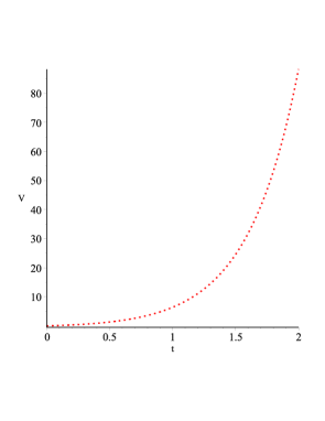
Figure 1: Evolution of the Universe filled with massive spinor field with $n_{1}=2/3$, $n_{2}=1/4$, $\lambda_{1}=1$ and $\lambda_{2}=1$

.

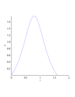
Figure 2: Evolution of the Universe filled with massive spinor field with $n_{1}=2/3$, $n_{2}=-1$, $\lambda_{1}=1$ and $\lambda_{2}=-1$.

.

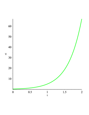
Figure 3: Evolution of the Universe filled with massive spinor field with $n_{1}=3/2$, $n_{2}=1/4$, $\lambda_{1}=-0.001$ and $\lambda_{2}=1$

.

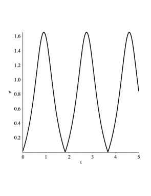
Figure 4: Evolution of the Universe filled with massive spinor field with $n_{1}=2/3$, $n_{2}=-1$, $\lambda_{1}=-0.001$ and $\lambda_{2}=-1$.

.

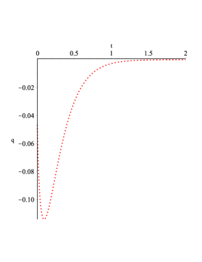
Figure 5: Plot of deceleration parameter $q$ with $n_{1}=2/3$, $n_{2}=1/4$, $\lambda_{1}=1$ and $\lambda_{2}=1$

.

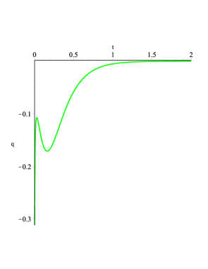
Figure 6: Plot of deceleration parameter $q$ with $n_{1}=3/2$, $n_{2}=1/4$, $\lambda_{1}=-0.001$ and $\lambda_{2}=1$.

.

IV Conclusion

Within the scope of Bianchi type-VI spacetime we study the role of spinor field on the evolution of the Universe. It is found that in this case the non-diagonal components of the energy-momentum tensor of spinor field, unlike in the cases Bianchi type I sahaAPSS2015 and Bianchi type-$VI_{0}$ sahabvi0 , does not lead to the elimination of spinor field nonlinearity and the mass term in spinor field Lagrangian. Depending of the sign of self-coupling constant the model in this case allows either late time acceleration or oscillatory mode of evolution.

Acknowledgments
This work is supported in part by a joint Romanian-LIT, JINR, Dubna Research Project, theme no. 05-6-1119-2014/2016.

References

• (1) A.G. Riess et al., Astron. J. 116, 1009 (1998)
• (2) S Perlmutter et al., Astrophys. J. 517, 565 (1999)
• (3) Sahni V. and Starobinsky A.A. Int. J. Mod. Phys. D 9 373 (2000)
• (4) Padmanabhan T. Phys. Rep. 380 235 (2003)
• (5) Saha B. Astrophys. Space Sci. 302 83 (2006) DOI: 10.1007/s10509-005-9008-5
• (6) Cardenas R., Gonzalez T., Leiva Y., Martin O. and Quiros I. Phys. Rev. D 67 083501 (2003)
• (7) Chimento L.P., Jakubi A.S., Pavon D., and Zimdahl W. Phys. Rev. D 67 083513 (2003)
• (8) Linder, E.V. General Relat. Grav. 40 329 (2008)
• (9) Olivares G., Atrio-Barandela F. and Pavon D. Phys. Rev. D 71 063523 (2005)
• (10) Zlatev I., Wang L., and Steinhardt P.J. Phys. Rev. Lett. 82 896 (1999)
• (11) Saha B Chinese J. of Phys. 43 1035 (2005)
• (12) Gorini V., Kamenshchik A., and Moschella U. Phys. Rev. D 67 063509 (2003)
• (13) Amendola L., Finelli F., Burigana C., and Carturan D. J. Cosmology Astropart. Phys. 0307 005 (2003)
• (14) Bean R. and Dore O. Phys. Rev. D. 68 023515 (2003)
• (15) Bento M.C., Bertolami O, and Sen A.A. Phys. Rev. D 66 043507 (2002)
• (16) Bento M.C., Bertolami O, and Sen A.A. Phys. Rev. D 67 063003 (2003)
• (17) Bento M.C., Bertolami O, and Sen A.A. Phys. Lett. B 575 172 (2003)
• (18) Biesiada M., Godlowski W., and Szydlowski M. Astrophys. J. 622 28 (2005)
• (19) Bilic N., Tupper G.B. and Viollier R.D. Phys. Lett. 353 17 (2002)
• (20) M. Henneaux Phys. Rev. D 21, 857 (1980)
• (21) U. Ochs and M. Sorg Int. J. Theor. Phys. 32, 1531 (1993)
• (22) B. Saha and G.N. Shikin Gen. Relat. Grav. 29, 1099 (1997)
• (23) B. Saha and G.N. Shikin J Math. Phys. 38, 5305 (1997)
• (24) B. Saha Phys. Rev. D 64, 123501 (2001)
• (25) B. Saha and T. Boyadjiev Phys. Rev. D 69, 124010 (2004)
• (26) B. Saha Phys. Rev. D 69, 124006 (2004)
• (27) B. Saha Phys. Particle. Nuclei. 37. Suppl. 1, S13 (2006)
• (28) B. Saha Grav. $\&$ Cosmol. 12(2-3)(46-47), 215 (2006)
• (29) B. Saha Romanian Rep. Phys. 59, 649 (2007).
• (30) B. Saha Phys. Rev. D 74, 124030 (2006)
• (31) C. Armend$\acute{a}$riz-Pic$\acute{o}$n and P.B. Greene Gen. Relat. Grav. 35, 1637 (2003)
• (32) M.O. Ribas, F.P. Devecchi, and G.M. Kremer Phys. Rev. D 72, 123502 (2005)
• (33) R.C de Souza and G.M. Kremer Class. Quantum Grav. 25, 225006 (2008)
• (34) G.M. Kremer and R.C de Souza arXiv:1301.5163v1 [gr-qc]
• (35) N. J. Popล‚awski Phys. Lett. B 690, 73 (2010)
• (36) N. J. Popล‚awski Phys. Rev. D 85, 107502 (2012)
• (37) N. J. Popล‚awski Gen. Releat. Grav. 44, 1007 (2012)
• (38) L. Fabbri Int. J. Theor. Phys. 52 634 (2013)
• (39) C.W. Misner Asrophys. J. 151, 431 (1968)
• (40) L. Fabbri Phys. Rev. D 85 0475024 (2012)
• (41) S. Vignolo, L. Fabbri, and R. Cianci J. Math. Phys. 52 112502 (2011)
• (42) V.G.Krechet, M.L. Felโ€™chenkov, and G.N. Shikin Grav. $\&$ Cosmol. 14 No 3(55), 292 (2008)
• (43) B. Saha Cent. Euro. J. Phys. 8, 920 (2010a)
• (44) B. Saha Romanian Rep. Phys. 62, 209 (2010b)
• (45) B. Saha Astrophys. Space Sci. 331, 243 (2011)
• (46) B. Saha Int. J. Theor. Phys. 51, 1812 (2012)
• (47) B. Saha Int. J. Theor. Phys. 53 1109 (2014) DOI: 10.1007/s10773-013-1906-7
• (48) B. Saha Astrophys. Space Sci. 357 28 (2015) DOI 10.1007/s10509-015-2291-x
• (49) B. Saha Euro. Phys. J. Plus 130 208 (2015) DOI 10.1140/epjp/i2015-15208-0
• (50) B. Saha and M. Visinescu, Romainan J. Phys. 55 1064 (2010)
• (51) Mohd. Zeyauddin and B. Saha, Astrophys. Space Sci. 343 445 (2013)
• (52) B. Saha, Int. J. Theor. Phys. 52 3646 (2013)
• (53) B. Saha, Phys. Part. Nuclei 45 349 (2014)
• (54) A. Pradhan and B. Saha, Phys. Part. Nuclei 46 310 (2015)
• (55) T.W.B. Kibble J. Math. Phys. 2, 212 (1961)
• (56) K.S. Thorne The Astrophys. J. 148, 51 (1967)
• (57) R. Kantowski and R.K. Sachs J. Math. Phys. 7, 443 (1966)
• (58) J. Kristian and R.K. Sachs Astrophys. J. 143, 379 (1966)
• (59) C.B. Collins, E.N. Glass, and D.A. Wilkinson Gen. Rel. Grav. 12, 805 (1980)