Fast bias inversion of a double well without residual particle excitation

Abstract

We design fast bias inversions of an asymmetric double well so that the lowest states in each well remain so and free from residual motional excitation. This cannot be done adiabatically, and a sudden bias switch produces in general motional excitation. The residual excitation is suppressed by complementing a predetermined fast bias change with a linear ramp whose time-dependent slope compensates for the displacement of the wells. The process, combined with vibrational multiplexing and demultiplexing, can produce vibrational state inversion without exciting internal states, just by deforming the trap.

I Introduction

In a recent paper multi a protocol to realize fast vibrational state multiplexing/demultiplexing of ultra cold atoms was introduced. By a properly designed time-dependent potential deformation between a harmonic trap and a biased double well, the states of a single atom in a harmonic trap can be dynamically mapped into states localized at each well (vibrational demultiplexing, see the left arrow in Fig. 1), or vice versa (multiplexing, see the right arrow in Fig. 1), faster than adiabatically and without residual excitation at the final time. It was suggested that these processes may be combined with a bias inversion to produce state inversions, from the ground to the first excited state of the harmonic trap and vice versa, based on trap deformations only, see Fig. 1, or to produce vibrationally excited Fock states from an initial ground state multi . These are basic operations to implement quantum information processing. Thus the possibility to perform them without exciting internal atomic states as an intermediate step is of much interest, as decoherence induced by decay would be suppressed; moreover the systems amenable of manipulation would not need to have an isolated two-level structure. The objective of this paper is to design fast controlled bias inversions so that the lowest states in each well remain so without residual excitation. Unlike multiplexing, however, there is no truly adiabatic slow process that achieves this state transformation. In the bias inversion depicted within the central frame of Fig. 1, for example, a slow bias change would preserve the state ordering so that the states represented in the third potential configuration would be interchanged (i.e. the grey state in the right well, and the white one in the left well). Nevertheless, in the limit in which the two wells are effectively independent, which in practice means, for times shorter than the tunneling time among the wells, the intended state transition might indeed be done slowly enough to be considered adiabatic. If we approximate each “isolated” well by a harmonic oscillator, the intended transformation amounts to a “horizontal” displacement along the inter well-axis together with a rising/lowering of the energy of the wells. The latter effects, however, do not affect the intrawell dynamics, so we may focus on the displacement. In other words, within the stated approximations the bias inversion amounts to the transport of a particle in a harmonic potential. Thus, to achieve a fast transition without residual excitation we may use shortcuts to adiabaticity designed to perform fast transport review . Specifically we shall use a compensating-force approach transport_Erik ; transport_Mikel , equivalent to the fast-forward scaling technique MN , based on adding to the potential a linear ramp with time-dependent slope to compensate for the effect of the trap motion in the non-inertial frame of the trap. We shall compare this approach with a sudden bias switch, a fast quasi-adiabatic (FAQUAD) approach FAQUAD , or a smooth polynomial connection without compensation. In Sec. II we introduce the compensating-force approach and Sec. III describes the alternative methods. In Sec. IV numerical examples are presented with parameters appropriate for trapped ions in multisegmented, linear Paul traps, and for neutral atoms in optical traps. Finally, in Sec. V we discuss the results and open questions.

Figure 1: Schematic representation of demultiplexing (left arrow), bias inversion (framed in dashed line, central arrow) and multiplexing (right arrow).

II Compensating-force approach

If the double well potential with nearly independent wells is subjected to a bias inversion such that the trap frequencies of each well are essentially equal and constant throughout, and the trajectories of the well minima move in parallel, the process may be described by a parallel transport of two rigid harmonic oscillators, one for each well. The Hamiltonian potential near the minima may be approximated as

$$V_{0}(x-x_{0})=\frac{1}{2}m\Omega_{0}^{2}(x-x_{0})^{2},$$ (1)

where $\Omega_{0}$ is the angular frequency and $x_{0}=x_{0}(t)$ is the common notation for either of the two minima. When needed we may distinguish the minima as $x_{0,\pm}$, with $x_{0,+}>x_{0,-}$. The Hamiltonian $H_{0}=p^{2}/2m+V_{0}(x-x_{0})$ has eigenenergies $E_{n}=\left(n+\frac{1}{2}\right)\hbar\Omega_{0},$ and well known normalized eigenstates $\phi_{n}(x-x_{0})$, proportional to Hermite polynomials Schiff .

Adding to the Hamiltonian a linear term with an appropriate time-dependent slope the non inertial effect of the motion of the well will be compensated in the trap frame transport_Erik ; transport_Mikel . To define the trap frame consider the following position and momentum displacement unitary operator

$$\mathcal{U}=e^{ipx_{0}(t)/\hbar}e^{-im\dot{x}_{0}(t)x/\hbar},$$ (2)

where the overdot represents a time derivative. Starting from the Schrödinger equation

$$i\hbar\partial_{t}|\psi\rangle=H_{0}|\psi\rangle,$$ (3)

the transformed wave function $|\Phi\rangle=\mathcal{U}|\psi\rangle$ obeys

$$i\hbar\partial_{t}|\Phi\rangle=\mathcal{U}H_{0}\mathcal{U}^{\dagger}|\Phi\rangle+i\hbar(\partial_{t}\mathcal{U})\mathcal{U}^{\dagger}|\Phi\rangle=H^{\prime}_{0}|\Phi\rangle,$$ (4)

where the interaction picture (trap frame) Hamiltonian is

$$H^{\prime}_{0}=\frac{p^{2}}{2m}+V_{0}(x)+mx\ddot{x}_{0}+\frac{1}{2}m{\dot{x}_{0}}^{2},$$ (5)

and $V_{0}(x)=\frac{1}{2}m\Omega_{0}^{2}x^{2}$. The term $m{\dot{x}_{0}}^{2}/2$ only depends on time, it does not affect the dynamics and can be ignored. To compensate the motion of the trap, we add $-mx\ddot{x}_{0}$ to $H_{0}$. This produces $-m(x+x_{0})\ddot{x}_{0}$ in the trap frame and the resulting potential in that frame is reduced to $V_{0}(x)$, again neglecting purely time-dependent functions. $V_{0}(x)$ does not depend on time, so any stationary state in this trap frame will remain stationary, an excitations are avoided.

III Alternative methods

In this section we present three simple alternative approaches to perform the bias inversion.

Sudden approach. In the sudden approach the potential is changed abruptly from the initial to the final configuration, but the state of the system remains unchanged immediately after the potential change (in general it will evolve afterwards). If the target state is $\psi_{tar}$ the resulting fidelity is

$$F_{s}=|\langle\psi(0)|\psi_{tar}\rangle|.$$ (6)

Fast quasi-adiabatic approach (FAQUAD). A quasi-adiabatic method to speed up adiabatic processes when there is one control parameter $\lambda(t)$ is based on distributing the adiabaticity parameter homogeneously in time FAQUAD . For instantaneous levels 0 and 1 this means

$$\hbar\left|\frac{{\langle}\phi_{0}|\partial_{t}\phi_{1}{\rangle}}{E_{0}-E_{1}}\right|=c,$$ (7)

where the instantaneous eigenstates $\phi_{0}$, $\phi_{1}$ and eigenenergies $E_{0}$, $E_{1}$ depend on time through their dependence on $\lambda$, and $c$ is constant. By the chain rule this becomes a first order differential equation for $\lambda(t)$, and $c$ is set so that the boundary conditions for $\lambda(t)$ at initial, $t=0$, and final time $t_{f}$ are satisfied. In the transport of a particle with a harmonic oscillator of angular frequency $\Omega_{0}$ centered at $x_{0}(t)$ we set $\lambda(t)=x_{0}(t)$. Using the energies and eigenstates of the first two levels of the harmonic oscillator in Eq. (7), the FAQUAD condition becomes simply

$$\frac{m\dot{x}_{0}(t)}{\sqrt{2\hbar m\Omega_{0}}}=c.$$ (8)

The solution is the linear connection $x_{0}(t)=x_{0}(0)+[x_{0}(t_{f})-x_{0}(0)]t/t_{f}$. The minimal $t_{f}$ for which a zero of excitation energy appears is Bowler ; FAQUAD $2\pi/\Omega_{0}$.

Polynomial connection without compensation. The final and initial values of the control parameter may as well be smoothly connected without applying any compensation, for example using a fifth order polynomial that assures the vanishing of first and second derivatives of the parameter at the boundary times.

IV Examples

In the following examples, the potentials and parameters are adapted for a trapped ion in a multisegmented Paul trap, and for a neutral atom in a dipole trap.

IV.1 Trapped ions

For a trapped ion we consider a simple double well potential of the form

$$V(x,t)=\beta x^{4}+\alpha x^{2}+\gamma x,$$ (9)

with $\alpha(t)<0$ and $\beta(t)>0$ Home ; Niza ; Mainz . $\alpha$ and $\beta$ are assumed to be constant and $\gamma\equiv\gamma(t)$ time dependent. The bias inversion implies a change of sign of $\gamma(t)$ from $\gamma_{0}>0$ to $-\gamma_{0}$.

From $\frac{\partial V}{\partial x}=0$ the condition for the extrema becomes

$$4\beta x^{3}+2\alpha x+\gamma=0.$$ (10)

It is useful to define

$$A = 0,\;B=\frac{2\alpha}{4\beta},\;C=\frac{\gamma}{4\beta},$$ (11)

$$Q = \frac{A^{2}-3B}{9},\,R=\frac{2A^{3}-9AB+27C}{54}.$$ (12)

When $R^{2}<Q^{3}$ there are two minima and one maximum. With $\alpha<0$ and $\beta>0$, this is satisfied for

$$|\gamma|<\left(\frac{2}{3}\right)^{3/2}\sqrt{-\frac{\alpha^{3}}{\beta}}.$$ (13)

The trajectories of the minima are

$$x_{0,\pm}=-2\sqrt{Q}\cos\left({\frac{\theta+(1\pm 1)\pi}{3}}\right)-\frac{A}{3},$$ (14)

where $\theta=\arccos\left({\frac{R}{\sqrt{Q^{3}}}}\right)$, $0\leq\theta\leq\pi$ and the roots are taken to be positive. Up to second order in $\gamma$ they are

$$x_{0,-} \approx -\frac{1}{\sqrt{2}}\sqrt{-\frac{\alpha}{\beta}}+\frac{\gamma}{4\alpha}-\frac{3\gamma^{2}\sqrt{-\alpha\beta}}{16\sqrt{2}\alpha^{3}},$$ (15)

$$x_{0,+} \approx \frac{1}{\sqrt{2}}\sqrt{-\frac{\alpha}{\beta}}+\frac{\gamma}{4\alpha}+\frac{3\gamma^{2}\sqrt{-\alpha\beta}}{16\sqrt{2}\alpha^{3}}.$$ (16)

The quadratic term $\gamma$ is negligible with respect to the linear term when

$$|\gamma|\ll\frac{4\sqrt{2}}{3}\sqrt{-\frac{\alpha^{3}}{\beta}},$$ (17)

which implies that the trajectories for the minima move in parallel. Note that this inequality automatically implies the one in Eq. (13). Neglecting the quadratic term, the two minima are given by $x_{0,\pm}=\pm\frac{1}{\sqrt{2}}\sqrt{-\frac{\alpha}{\beta}}+\frac{\gamma}{4\alpha}$. The distance between the minima is given by

$$D = 2\sqrt{Q}\left\{\cos{\left(\frac{\theta}{3}\right)}+\sin{\left[\frac{1}{6}(\pi+2\theta)\right]}\right\}$$ (18)

$$\approx \sqrt{2}\sqrt{-\frac{\alpha}{\beta}}+\frac{3\sqrt{-\alpha\beta}}{8\sqrt{2}\alpha^{3}}\gamma^{2}.$$

We may also compute the energy bias between the two wells as

$$\delta=\gamma D.$$ (19)

The distance travelled by each well is, when (17) is fulfilled, $d=\gamma_{0}/(2\alpha)$, see Eqs. (15) and (16), and the effective frequency at each minimum

$$\omega_{0}=\sqrt{\frac{1}{m}\left(\frac{d^{2}V}{dx^{2}}\right)_{x=x_{0}}}.$$ (20)

For Eq. (9) the effective frequencies are

$$\omega_{0,\pm} = \sqrt{\!\frac{2}{m}}\sqrt{\!\alpha\!+\!\frac{2}{3}\beta\left\{\!A\!+\!6\sqrt{Q}\cos\!{\left[\frac{1}{3}\!\left(\!\frac{\theta+(1\pm 1)\pi}{3}\!\right)\!\right]}\!\right\}^{\!2}\!}$$ (21)

$$\approx 2\sqrt{-\frac{\alpha}{m}}\mp\frac{3}{2\sqrt{2}}\sqrt{\frac{\beta}{\alpha^{2}m}}\gamma.$$

Hence, comparing the two terms, the condition for the frequencies to be essentially constant $\omega_{0,\mp}\approx\Omega_{0}\equiv 2\sqrt{-\frac{\alpha}{m}}$ is again the inequality in Eq. (17).

In the regime where the inequality (17) holds, we can apply the compensating force approach to implement a fast bias inversion. Since the compensating term $-mx\ddot{x}_{0}$ is equal for both harmonic traps, we add it to $V$ in Eq. (9), and the resulting Hamiltonian $H$ is

$$H=\frac{p^{2}}{2m}+\beta x^{4}+\alpha x^{2}+(\gamma-m\ddot{x}_{0})x.$$ (22)

Note that the compensation amounts to changing the time dependence of the slope of the linear term from the reference process defined by $\gamma(t)$ to $\gamma_{eff}(t)\equiv\gamma(t)-m\ddot{x}_{0}(t)=\gamma(t)-m\ddot{\gamma}(t)/(4\alpha)$. To set $\gamma(t)$ we design a connection between the initial and final configurations. First note the boundary conditions

$$\gamma(0)=\gamma_{0}>0,\,\,\,\gamma(t_{f})=-\gamma_{0},$$ (23)

which we complement by

$$\dot{\gamma}(t_{b})=0,\,\,\,\ddot{\gamma}(t_{b})=0,$$ (24)

$$t_{b}=0,t_{f},$$

so that $\dot{x}_{0}(t_{b})=\ddot{x}_{0}(t_{b})=0$. This implies that ${\cal{U}}(t_{b})=e^{ipx_{0}(t_{b})/\hbar}$ and $\dot{\cal{U}}(t_{b})=0$. Therefore the Hamiltonians and the wave functions in interaction and Schrödinger pictures transform into each other by a simple coordinate displacement. At intermediate times, we interpolate the function as $\gamma(t)=\sum_{n=0}^{5}c_{n}t^{n}$, where the coefficients are found by solving Eqs. (23) and (24). Finally,

$$\gamma(t) = \gamma(0)+10[\gamma(t_{f})-\gamma(0)]s^{3}$$ (25)

$$- 15[\gamma(t_{f})-\gamma(0)]s^{4}+6[\gamma(t_{f})-\gamma(0)]s^{5},$$

where $s=t/t_{f}$. This function and examples of $\gamma_{eff}$ are shown in Fig. 2.

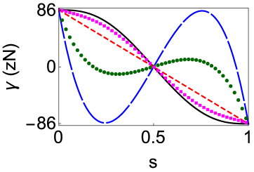
Figure 2: (Color online) $\gamma$ versus $s=t/t_{f}$ for the polynomial in Eq. (25) (solid black line) and FAQUAD (short-dashed red line). $\gamma_{0}=86.4$ zN, $\gamma(t_{f})=-\gamma_{0}$, $\alpha=-4.7$ pN/m, and $\beta=5.2$ mN/m³. Also shown are the different effective slopes adding a compensation to the polynomial, $\gamma_{eff}(t)=\gamma(t)-m\ddot{\gamma}(t)/(4\alpha)$, for the mass of ⁹Be⁺ and times $t_{f}=0.07$ $\mu$s (long-dashed blue line); $t_{f}=0.1$ $\mu$s (green dots); and $t_{f}=0.3$ $\mu$s (magenta squares).

In order to compare the robustness of the compensating force method against the alternative ones we consider a ⁹Be⁺ ion in the double well with the realistic parameters $\alpha=-4.7$ pN/m and $\beta=5.2$ mN/m³, similar to those in Wineland . For a moderate initial bias compared to the vibrational quanta, such as

$$\gamma_{0}\sim\frac{\hbar\Omega_{0}}{D},$$ (26)

the fidelity provided by the sudden approach is one for all practical purposes so we can change the bias abruptly and reach the target state. The displacement of the trap $d$ may be compared with the oscillator characteristic length $a_{0}=\sqrt{\hbar/m\Omega_{0}}$. Their ratio is

$$R=\frac{d}{a_{0}}=\frac{\gamma_{0}}{2\alpha}\sqrt{\frac{m\Omega_{0}}{\hbar}}.$$ (27)

For the Paul trap $R\approx 0.00065$, which explains the high fidelity of the sudden approach for a moderate bias inversion of the ion. At these bias values there is really no need to apply a more sophisticated protocol than the sudden switch.

Henceforth, we assume a much larger $\gamma_{0}$, but still satisfying the condition (17). In particular, for an initial bias of 1000 $\Omega_{0}\hbar$ (corresponding to $\gamma_{0}=86.4$ zN), the ratio becomes $R\approx 0.65$. The maximum variation of the difference between the trajectories of the minima is $3$ pm, about three orders of magnitude less than the displacement of each minimum ($9.2$ nm), so the minima follow parallel trajectories. Furthermore, the maximum variation of the frequencies in Eq. (21) with respect to $\Omega_{0}=2\pi\times 5.6$ MHz is $2\pi\times 3.7$ kHz, so the effective frequency is nearly constant.

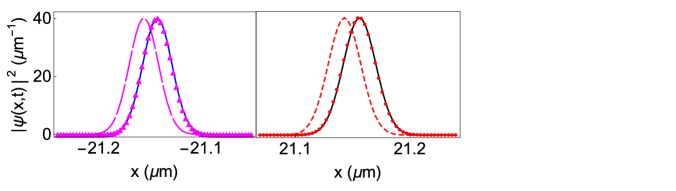
Figure 3: (Color online) Left: Ground state of the left well at $t=0$ (long-dashed magenta line) and at $t=t_{f}$ (magenta triangles), and final state with the compensating force applied on the double well (solid blue line). Right: Ground state of the right well: at $t=0$ (short-dashed red line) and at $t=t_{f}$ (red dots) and final state with the compensating force applied (solid black line). $t_{f}=4$ ns and other parameters as in Fig. 2 for ⁹Be⁺.

Figure 3 demonstrates the effect of the compensating-force approach. Starting from the ground state of the lower (left) well, the final evolved state following the shortcut with compensation stays as the “ground state” of the left well. This is actually defined as the lowest state of the double well system predominantly located on the left. There is a similar process for the right well. The final states represented are obtained by solving the Schrödinger equation with the full Hamiltonian (22).

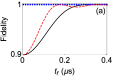
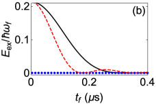
Figure 4: (Color online). (a) Fidelity $|\langle\phi_{L}(t_{f})|\psi(t_{f})\rangle|$, where $|\phi_{L}(t_{f})\rangle$ is the lowest state located in the left well in the final time configuration, and $|\psi(t_{f})\rangle$ is the evolved state following the shortcut at final time. (b) Final excitation energy for the process on the left well using compensating-force (blue dots), fifth degree polynomial in Eq. (25) (solid black line), and FAQUAD (short-dashed red line). The parameters are for ⁹Be⁺ as in Fig. 2.

Fig. 4 is for the process in the left well. It compares the fidelity at final time and the excitation energy, defined as $E_{ex}=E(t_{f})-E_{0}(t_{f})$ where $E(t_{f})$ is the final energy after the quantum evolution following the shortcut and $E_{0}(t_{f})$ is the ground state final energy of the upper harmonic well, using the polynomial (25) for $\gamma$ with and without compensation, as well as the results of the FAQUAD approach. The fidelity without compensation tends to the fidelity of the sudden approach ($0.89$) for very short final times. The method with compensation clearly outperforms the others. In principle a fundamental limitation of the approach is due to the fact that the inequality (17), that guarantees parallel motion and stable frequencies of the wells, should as well be satisfied by $\gamma_{eff}$, but, at very short times, the dominant term of $\gamma_{eff}\sim-m\ddot{\gamma}/{4\alpha}$ may be too large. To estimate this short time limit we combine the mean-value theorem inequality for the maximum transport_Erik , $|\ddot{\gamma}|_{max}\geq 4\gamma_{0}/t_{f}^{2}$, with Eq. (17) for $\gamma_{eff}$ to find the condition

$$t_{f}>>\left(\frac{3m\gamma_{0}}{4\sqrt{2}}\sqrt{-\frac{\beta}{\alpha^{5}}}\right)^{1/2}.$$ (28)

The factor on the right hand side is $10^{-9}$ s for this example, see Fig. 4, which is several orders of magnitude smaller than $2\pi/\Omega_{0}$ and does not affect the fidelity in the scale of times shown.

IV.2 Neutral atoms

The potential

$$V_{na}(x,t)=\frac{1}{2}m\omega^{2}x^{2}+V_{0}\cos^{2}\left[\frac{\pi(x-\Delta x)}{d_{l}}\right].$$ (29)

forms also a double well. It was implemented in Oberthaler with optical dipole potentials, combining a harmonic confinement due to a crossed beam dipole trap with a periodic light shift potential provided by the interference pattern of two mutually coherent laser beams. $\omega$ is the angular frequency of the dipole trap about the waist position, $V_{0}$ the amplitude, $\Delta x$ the displacement of the optical lattice relative to the center of the harmonic well, and $d_{l}$ is the lattice constant. (Double wells with a controllable bias may be also realized by two optical lattices of different periodicity with controllable intensities and relative phase Bloch .) Here, the bias inversion implies a change of sign of $\Delta x(t)$ from $\Delta x_{0}>0$ to $-\Delta x_{0}$.

To check if the conditions to apply the compensating force approach hold here as well, an analysis similar to the one in the previous example is now performed. We approximate the potential around each minimum, $V^{(\pm)}$, up to fourth order. From $\frac{\partial V^{(\pm)}}{\partial x}=0$ we get a cubic equation for each minimum. The positions of the minima are thus given by

$$x_{0,\pm}=-2\sqrt{Q}\cos{\left(\frac{\theta^{(\pm)}-2\pi}{3}\right)}-\frac{A^{(\pm)}}{3},$$ (30)

where

$$Q = \frac{2d_{l}^{2}\pi^{2}V_{0}+d_{l}^{4}m\omega^{2}}{4\pi^{4}V_{0}},$$

$$A^{(\pm)} = -\frac{3}{2}(2\Delta x\pm d_{l}),$$

$$\theta^{(\pm)} = \cos{\left[\frac{-3d_{l}(2\Delta x\pm d_{l})m\pi^{2}\sqrt{V_{0}}\omega^{2}}{2(2\pi^{2}V_{0}+d_{l}^{2}m\omega^{2})^{3/2}}\right]}^{-1}.$$ (31)

Up to a second order in $\Delta x$,

$$x_{0,\pm}\approx\pm a+b\Delta x\pm c\Delta x^{2},$$ (32)

where the coefficients are known explicitly but too lengthy to be displayed here. Whenever the quadratic term is negligible with respect to the linear term ($c\Delta x^{2}<<b\Delta x$), we can approximate $x_{0,\pm}=\pm a+b\Delta x$ (parallel motion). The distance between the minima is given by

$$D = \frac{1}{3}\left\{A^{(-)}-A^{(+)}+6\sqrt{Q}\left[-\cos{\left(\frac{\pi+\theta^{(-)}}{3}\right)}\right.\right.$$ (33)

$$+ \left.\left.\cos{\left(\frac{\pi+\theta^{(+)}}{3}\right)}\right]\right\}\approx 2a+2c\Delta x^{2}.$$

Moreover, $\omega_{0,\pm}\approx f\mp g\Delta x$, again with known but lengthy coefficients $g$ and $f$. As long as $g\Delta x<<f$ we may set $\omega_{0,\pm}\approx\Omega_{0}\equiv f$.

For realistic parameters the conditions for parallel transport of the minima and constant frequency are indeed satisfied. We consider a ⁸⁷Rb atom in the trap and set the parameters in multi after the demultiplexing process, namely, $d_{l}=5.18$ $\mu$m, $\omega=2\pi\times 59.4$ Hz, and $V_{0}/h=1.4$ kHz; the time-dependent displacement $\Delta x=\Delta x(t)$ is the control parameter to perform the bias inversion, such that

$$\Delta x(0)=\Delta x_{0},\,\,\,\Delta x(t_{f})=-\Delta x_{0},$$ (34)

with $\Delta x_{0}=200$ nm. We also impose

$$\dot{\Delta}x(0)=0,\,\,\,\ddot{\Delta}x(0)=0,$$

$$\dot{\Delta}x(t_{f})=0,\,\,\,\ddot{\Delta}x(t_{f})=0,$$ (35)

to achieve similar conditions in the derivatives of the minima $x_{0}$. At intermediate times, we interpolate the function as $\Delta x(t)=\sum_{n=0}^{5}d_{n}t^{n}$, where the coefficients are found by solving Eqs. (34) and (IV.2). Consequently, the connection between the initial and final Hamiltonians is given by the same polynomial in Eq. (25) changing $\gamma(t)\to\Delta x(t)$. The double wells are much deeper and tight for trapped ions than for neutral atoms, compare an intrawell angular frequency $\Omega_{0}$ of $2\pi\times 5.6$ MHz for the ions versus $2\pi\times 0.35$ kHz for the optical trap. Therefore, in this case, for a moderate initial bias compared to the vibrational quanta, the ratio between the displacement of the trap $d$ and the oscillator characteristic length $a_{0}$ is $R\approx 0.67$.

With the parameters given at time $t=0$, the separation of the minima is $D=5$ $\mu$m, the bias between minima $\delta=2.02\times 10^{-32}$ J, and an the effective angular frequency $\Omega_{0}=2\pi\times 0.35$ kHz, whereas the maximum variation of the frequencies along the process is approximately $2\pi\times 0.2$ Hz. Furthermore, the maximum deviation from $D$ of the minima separation is $1.8$ nm, whereas the displacement of each minimum is about $0.4$ $\mu$m. In summary the minima do move in parallel with constant, equal frequencies for practical purposes.

To accelerate the bias inversion we add the compensating term to $V$ in Eq. (29),

$$H=\frac{p^{2}}{2m}+\frac{1}{2}m\omega^{2}x^{2}+V_{0}\cos^{2}\left[\frac{\pi(x-\Delta x)}{d_{l}}\right]-mx\ddot{x}_{0}.$$ (36)

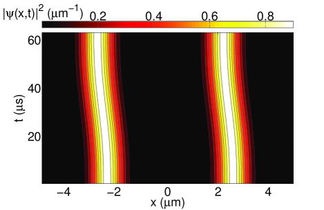
Figure 5: (Color online) Evolution of the wave function densities following the shortcut in Eq. (36) for states in left and right wells. The parameters are for ⁸⁷Rb: $d_{l}=5.18$ $\mu$m, $\omega=59.4\times 2\pi$ Hz, $V_{0}/h=1.4$ kHz, $\Delta x_{0}=200$ nm, and $t_{f}=63$ $\mu$s.

Figure 5 shows the evolution of the densities.

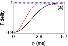
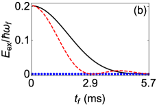
Figure 6: (Color online). (a) Fidelity $|\langle\varphi_{1}(t_{f})|\psi(t_{f})\rangle|$, where $|\varphi_{1}(t_{f})\rangle$ is the lowest state predominantly of the left well at final time (the first excited state of the double well) and $|\psi(t_{f})\rangle$ is the evolved state following the shortcut at final time. (b) Final excitation energy. Compensating-force approach (blue dots), fith degree polynomial in Eq. (25) with the change $\gamma(t)\to\Delta x(t)$ without compensation (solid black line), and FAQUAD approach (short-dashed red line). The parameters are chosen for ⁸⁷Rb: $d_{l}=5.18$ $\mu$m, $\omega=59.4\times 2\pi$ Hz, $V_{0}/h=1.4$ kHz, and $\Delta x_{0}=200$ nm.

Focusing on the left well, Fig. 6 (a) demonstrates that the fidelity is exactly one (blue dots) with the compensating force. However, using for the inversion the fifth degree polynomial in Eq. (25) (with the change $\gamma(t)\to\Delta x(t)$) without compensation the fidelity at short final times decreases until the value of the sudden approach, 0.9. Furthermore, the excitation (residual) energy $E_{ex}$ is approximately zero for the shortcut protocol, compared to the excitation without compensation in Fig. 6 (b). In practice, the minimal process times $t_{f}$ are not limited by the method per se but by the technical capabilities to implement the maximal compensating force. This force depends on the maximal acceleration of the well, whose lower bound is known to be $a_{\rm max}=2d/t^{2}_{f}$ transport_Erik . To implement the compensation with a magnetic field gradient $G$, the gradient should be of the order of $G\simeq ma_{\rm max}/\mu_{B}$ in an amount of time $t_{f}$ ($\mu_{B}$ is Bohr’s magneton). For rubidium atoms polarized in the magnetic level $F=m_{F}=2$ and the transport parameters considered above, this requires a magnetic field gradient on the order of $40$ T/m shaped on a time interval $t_{f}=63$ $\mu$s. This is definitely challenging from an experimental point of view. Alternatively, one can use the dipole force of an out of axis Gaussian laser beam. If the double well is placed on the edge at a distance of $w/2$ where $w$ is the waist and if $\alpha_{p}$ denotes the polarizability, the local potential slope experienced by the atoms is on the order of $\alpha_{p}P/w^{3}$ where $P$ is the power of the beam. The compensation requires that $P/w^{3}=m/\alpha_{p}$. For instance, with an out-of-resonance beam at a wave length of 1 $\mu$m, the polarizability of rubidium-87 atoms is $\alpha_{p}\simeq 1.3\times 10^{-36}$ m²s, and the compensation can be performed using a 1W laser with a waist of 20 $\mu$m.

V Discussion

In this work we have proposed a method to invert the bias of a double-well potential, in the regime of independent wells, to keep the final states motionally unexcited within the same original well. The method treats the bias inversion as a rigid transport of the wells, which is justified for realistic parameters, and applies a “compensating-force” to cancel the excitations. Examples have been worked out for ions or neutral atoms and comparisons have been provided with a sudden approach, a fast quasi-adiabatic (FAQUAD) approach, or a smooth polynomial connection of initial and final bias without compensation. The compensating-force method clearly outperforms the others and gives ideally perfect fidelities, at least under ideal conditions, up to very small times compared e.g. with the time $2\pi/\Omega_{0}$ where FAQUAD provides a first zero of excitation.

One more advantage is the flexibility, as the reference process used to design the corresponding compensation (we have used a polynomial for simplicity) may be chosen among a broad family of functions satisfying Eqs. (23, 24). As in other shortcut approaches, this flexibility may be used to enhance robustness versus noise and perturbations error ; Lu ; DavidGon .

The bias inversion put forward here and the multiplexing and demultiplexing protocols developed in multi provide the necessary toolkit to perform vibrational state inversions Jurgen ; Jurgen2 , or Fock state preparations multi . Applications in optical waveguide design are also feasible optical . As well, the fast bias inversion is directly applicable to Bose-Einstein condensates Masuda2 ; transcond .

Generalizations for conditions in which rigid transport does not hold are also possible using invariant theory transport_Erik , which allows for finding processes without final excitation where both the frequency and position of the well depend on time new .

References

- (1) S. Martínez-Garaot, E. Torrontegui, X. Chen, M. Modugno, D. Guéry-Odelin, S.-Y. Tseng, and J. G. Muga, Phys. Rev. Lett. 111, 213001 (2013).
- (2) E. Torrontegui, S. Ibáñez, S. Martínez-Garaot, M. Modugno, A. del Campo, D. Guéry-Odelin, A. Ruschhaupt, X. Chen, and J. G. Muga, Adv. At. Mol. Opt. Phys. 62, 117 (2013).
- (3) E. Torrontegui, S. Ibáñez, X. Chen, A. Ruschhaupt, D. Guéry-Odelin, and J. G. Muga, Phys. Rev. A 83, 013415 (2011).
- (4) M. Palmero, E. Torrontegui, D. Guéry-Odelin, and J. G. Muga, Phys. Rev. A 88, 053423 (2013).
- (5) S. Masuda and K. Nakamura, Proc. R. Soc. A 466, 1135 (2010).
- (6) S. Martínez-Garaot, A. Ruschhaupt, J. Gillet, Th. Busch, and J. G. Muga, arXiv:1411.5783 (2014).
- (7) L. I. Schiff, Quantum mechanics (McGraw-Hill, New York, 1981).
- (8) R. Bowler, J. Gaebler, Y. Lin, T. R. Tan, D. Hanneke, J. D. Jost, J. P. Home, D. Leibfried, and D. J. Wineland, Phys. Rev. Lett. 109, 080502 (2012).
- (9) J. P. Home and A. M. Steane, Quantum Inf. Comput. 6, 289 (2006).
- (10) A. H. Nizamani and W. K. Hensinger, Appl. Phys. B 106, 327 (2012).
- (11) H. Kaufmann, T. Ruster, C. T. Schmiegelow, F. Schmidt-Kaler F, and U. G. Poschinger, New J. Phys. 16, 073012 (2014).
- (12) A. C. Wilson, Y. Colombe, K. R. Brown, E. Knill, D. Leibfried and D. J. Wineland, Nature 512, 57-60 (2014).
- (13) R. Gati, M. Albiez, J. Fölling, B. Hemmerling, and M. K. Oberthaler, Appl. Phys. B 82, 207 (2006).
- (14) S. Fölling, S. Trotzky, P. Cheinet, M. Feld, R. Saers, A. Widera, T.Müller, and I. Bloch, Nature (London) 448, 1029 (2007).
- (15) A. Ruschhaupt, X. Chen, D. Alonso and J. G: Muga, New J. Phys. 14, 093040 (2012).
- (16) X.-J. Lu, J. G. Muga, X. Chen, U. G. Poschinger, F. Schmidt-Kaler, and A. Ruschhaupt, Phys. Rev. A 89, 063414 (2014).
- (17) D. Guéry-Odelin and J. G. Muga, Phys. Rev. A 90, 063425 (2014).
- (18) R. Büker, T. Berrada, S. van Frank, J.-F. Schaff, T. Schumm, J. Schmiedmayer, G. Jäger, J. Grond, and U. Hohenester, J. Phys. B 46, 104012 (2013).
- (19) R. Bücker, J. Grond, S. Manz, T. Berrada, T. Betz, C. Koller, U. Hohenester, T. Schumm, A. Perrin, and Jörg Schmiedmayer, Nat. Phys. 7, 608 (2011).
- (20) S.-Y. Tseng and X. Chen, Opt. Lett. 37, 5118 (2012).
- (21) S. Masuda, Phys. Rev. A 86, 063624 (2012).
- (22) E. Torrontegui, X. Chen, M. Modugno, S. Schmidt, A. Ruschhaupt, and J. G. Muga, New J. Phys. 14, 013031 (2012).
- (23) M. Palmero and J. G. Muga, in preparation.