Towards a statistical mechanical theory of active fluids

Abstract

We present a stochastic description of a model of $N$ mutually interacting active particles in the presence of external fields and characterize its steady state behavior in the absence of currents. To reproduce the effects of the experimentally observed persistence of the trajectories of the active particles we consider a Gaussian forcing having a non vanishing correlation time $\tau$, whose finiteness is a measure of the activity of the system. With these ingredients we show that it is possible to develop a statistical mechanical approach similar to the one employed in the study of equilibrium liquids and to obtain the explicit form of the many-particle distribution function by means of the multidimensional unified colored noise approximation. Such a distribution plays a role analogous to the Gibbs distribution in equilibrium statistical mechanics and provides a complete information about the microscopic state of the system. From here we develop a method to determine the one and two-particle distribution functions in the spirit of the Born-Green-Yvon (BGY) equations of equilibrium statistical mechanics. The resulting equations which contain extra-correlations induced by the activity allow to determine the stationary density profiles in the presence of external fields, the pair correlations and the pressure of active fluids. In the low density regime we obtain the effective pair potential $\phi(r)$ acting between two isolated particles separated by a distance, $r$, showing the existence an effective attraction between them induced by activity. Based on these results, in the second half of the paper we propose a mean field theory as an approach simpler than the BGY hierarchy and use it to derive a van der Waals expression of the equation of state.

I Introduction

The collective behavior of microscopic living organisms and active particles capable of transforming chemical energy into motion has recently attracted the attention of the soft-condensed matter community as they present striking analogies, but also intriguing differences with respect to colloidal and molecular fluids Romanczuk et al. (2012); Elgeti et al. (2014); Marchetti et al. (2013); Ramaswamy (2010). Can we understand their rich phenomenology by applying experimental, theoretical and numerical techniques which proved to be successful in condensed matter physics? Recent investigations based on physical models akin to those widely employed in statistical mechanics, thermodynamics and rheology seem to give support to this hypothesis.

Among the most studied systems we mention swimming bacteria, colloidal particles immersed in bacterial suspensions and self-propelled Janus particles. Swimming bacteria can be schematized as objects moving with speed $v_{0}$ along straight paths of average duration $\tau$, the so called persistence time, after which a random reorientation (a tumble) takes place. After many such events, i.e. on a time scale larger than $\tau$, the particle displacement can be assimilated to a random walk and diffusive behavior emerges with a diffusion constant, $D_{a}=v_{0}^{2}\tau/2d$, where $d$ is the space dimensionality. The resulting motion displays two peculiar features: a) the trajectories display an anomalously long persistence not observed in Brownian motion, i.e. their direction and the velocity remain constant for a time lapse much longer than those corresponding to colloidal particles, and the similarity with ordinary diffusion appears only on a longer time-scale; b) there is a spontaneous tendency of the particles to aggregate into clusters notwithstanding there is no evidence of direct attractive forces, while on the contrary short repulsive inter-particle forces are at work. This is in a nutshell the idea of the successful run-and-tumble (RnT) model that captures many aspects experimentally observed Berg (2004); Schnitzer (1993); Tailleur and Cates (2008). Experiments conducted employing swimming bacterial suspensions have shown that their diffusivity can be hundred times larger than the one arising from the thermal agitation Valeriani et al. (2011); Di Leonardo et al. (2010); Schwarz-Linek et al. (2012). To give some numbers the diffusivity of Escherichia coli bacteria is $D\approx 100\,\mu m^{2}/s$, whereas passive bacteria diffuse with $D\approx 0.3\,\mu m^{2}/s$. Active Janus particles instead have $D$ in a range $4-25\,\mu m^{2}/s$, finally colloidal particles immersed in a bacterial suspension display $D\approx 0.5-0.1\,\mu m^{2}/s$. In all cases, the contribution due to the diffusion due to the thermal agitation of the molecules of the solvent is more than ten times smaller than the one due to the activity Poon (2013).

The work of several groups has led to the formulation of theoretical models and to the application of methods of statistical mechanics Cates (2012); Bialké et al. (2014); Smallenburg and Löwen (2015); Baskaran and Marchetti (2010); Fily and Marchetti (2012); Stenhammar et al. (2013), whereas Brady and Takatori Takatori and Brady (2014) have put forward an approach based on thermodynamics and microrheology and introduced the seminal idea of swim temperature $T_{s}$ and swim pressure $T_{s}\rho$, $\rho$ being the particle number density. In addition to the swim pressure, the total pressure contains other contributions stemming not only from the particle excluded volume but also from the effective attraction experienced by the active particles. Such an effective attraction is a peculiar aspect of active matter: motile particles, characterized by isotropic repulsive interactions due to the persistence of their motions become slower at high density and tend to form clusters and/or pile-up in regions adjacent repulsive substrates. The attractive forces may eventually lead to a scenario where van der Waals loops appear as soon as the off-equilibrium control parameter, the persistence time, is above a certain critical value.

The idea of the present paper is to use a microscopic model capable of reproducing the basic features of the RnT model and of the active Brownian particles. In our model the microscopic state is specified only by the particles positions, while the effect of the angular dynamics is encapsulated in a Gaussian colored noise having a finite relaxation time, reflecting the persistence of the directions. The correspondence between the models can be established by noting that, in the free particle case, in all models each velocity component has an exponential time-autocorrelation function characterized by a correlation time $\tau$  Koumakis et al. (2014); Maggi et al. (2014, 2015); Farage et al. (2015). Despite the differences in the driving stochastic forces, as shown in Ref. Maggi et al. (2015), Gaussian-colored noise driven particles behave strikingly similarly to RnT particles when in presence of steeply repulsive interactions. Moreover the Gaussian colored noise model is the only one for which an approximate stationary distribution for multiple particles is known Maggi et al. (2015). This motivates us further in studying the Gaussian colored noise model in more detail.

Somehow surprisingly the present work shows that the approximate stationary configurational distribution of a system of interacting particles undergoing over-damped motion under the action of Gaussian colored noise bears a strong resemblance with the equilibrium Gibbs distribution Tailleur and Cates (2008); Cates (2012), with the due differences: a new temperature, named swim temperature, takes the role of the ordinary temperature, the probability of configurations depends on a complicated function of ${\cal U}$, the potential energy. Such a result is independent on the fine details of the interactions, but certainly depends on the persistence of the random fluctuations. The most direct consequence of the form of this steady state distribution is the appearance of an effective attraction between two or more active particles in the absence of any attractive direct interaction Angelani et al. (2011). The reduction of the mobility of the particles due to the presence of other particles in their vicinity may eventually lead to a phase separation between a high and a rarefied density phase, a phenomenon named motility induced phase separation (MIPS) Tailleur and Cates (2008); Cates and Tailleur (2014).

This paper is organized as follows: in Sec. II we present the coarse grained stochastic model describing an assembly of active particles, consisting of a set of coupled Langevin equations for the coordinates of the particles subject to colored Gaussian noise. We switch from the Langevin description to the corresponding Fokker-Planck equation for the joint probability distribution of $N$ particles and within the multidimensional unified colored noise approximation (MUCNA) Hanggi and Jung (1995); Maggi et al. (2015), in the stationary case and under the condition of vanishing currents we obtain its exact form. The obtained distribution implies detailed balance and potential conditions as discussed in appendix C. In the case of non vanishing currents it is straightforward to write such a distribution for a single particle in one dimension in the presence of colored noise Lindner et al. (1999), whereas in higher dimensions and in interacting systems sucha a generalization cannot be obtained by the method of appendix A. Using the $N$-particle distribution in Sec. III we derive the first two members of a hierarchy of equations for the marginalized probability distributions of one and two particles that play the role of the Born-Green-Yvon (BGY) equations for active systems. We apply the first of these equations to the study of a density profile in the presence of an external potential, extend the treatment to the case of interacting active particles. In the low density limit we are able to write the exact form of such the pair correlation and define the effective pair potential between two isolated particles. In section IV we employ a variational approach, complementary to that based on the BGY equations which are exact but highly unpractical, and taking advantage of the explicit form of the MUCNA equation we construct a "free energy" functional whose minimum corresponds to the exact solution. The mean-field theory for interacting systems follows by searching the solution among the probability distributions which are a product of single particle probability distributions. The functional is finally used in section V to lay out a method capable to interpret the phase behavior of the model in terms of the relevant control parameters starting from a microscopic description. Finally, we present our conclusions in VI. We include with four appendices: in appendix A containing the calculation details leading to the MUCNA, in appendix B we discuss the approach to the solution and establish an H-theorem, in appendix C we verify the detailed balance condition, whereas in appendix D we discuss a technical aspect which allows to evaluate a key ingredient of our approach, the determinant of the friction matrix.

II The model and its stationary many-particle distribution function

In order to describe the properties of a suspension of active particles we consider a three dimensional container of volume $V$ where an assembly of $N$ interacting active spherical particles at positions ${\bf r}_{i}$, with $i$ ranging from 1 to $N$, subject to external fields undergoes over-damped motion driven by random fluctuating forces of different origin and nature. In fact, each particle besides experiencing a white noise force, due to the thermal agitation of the solvent and characterized by a diffusivity $D_{t}$ , is acted upon by a drag force proportional to its velocity, $\dot{\bf r}_{i}$, and in addition is subject to a colored Gaussian noise, $\boldsymbol{v}_{i}$, of zero mean, characteristic time $\tau$ and diffusivity $D_{a}$. This second type of noise is intended to mimic on time scales larger than $\tau$ the behavior of self-propelled particles whose propulsion force randomizes with characteristic time $\tau$. Such a model involving only the positional degrees of freedom of the particles has the advantage of allowing for analytical progress and for this reason can be used instead of more microscopic models where the rotational dynamics is fully accounted for. We consider the following set of equations of motion for the positions of the active Brownian spheres which has been treated in the literature by some authors Farage et al. (2015); Elgeti et al. (2014); Maggi et al. (2015) :

$$\dot{{\bf r}}_{i}(t)=\frac{1}{\gamma}\boldsymbol{F}_{i}({\bf r}_{1},\dots,{\bf r}_{N})+D_{t}^{1/2}\boldsymbol{\xi}^{t}_{i}(t)+\boldsymbol{v}_{i}(t)$$ (1)

are coupled to changes of the velocities $\boldsymbol{v}$ described by:

$$\dot{\boldsymbol{v}}_{i}(t)=-\frac{1}{\tau}\boldsymbol{v}_{i}(t)+\frac{D_{a}^{1/2}}{\tau}\boldsymbol{\eta}_{i}(t)$$ (2)

The force $\boldsymbol{F}_{i}=-\nabla_{i}{\cal U}$ acting on the $i$-th particle is conservative and associated to the potential ${\cal U}({\bf r}_{1},\dots,{\bf r}_{N})$, $\gamma$ is the drag coefficient, whereas the stochastic vectors $\boldsymbol{\xi}^{t}_{i}(t)$ and $\boldsymbol{\eta}_{i}(t)$ are Gaussian and Markovian processes distributed with zero mean and moments $\langle\boldsymbol{\xi}^{t}_{i}(t)\boldsymbol{\xi}^{t}_{j}(t^{\prime})\rangle=2\delta_{ij}\delta(t-t^{\prime})$ and $\langle\boldsymbol{\eta}_{i}(t)\boldsymbol{\eta}_{j}(t^{\prime})\rangle=2\delta_{ij}\delta(t-t^{\prime})$. While $D_{t}$ represents a translational diffusion coefficient, the coefficient $D_{a}$ due to the activity is related to the correlation of the Ornstein-Uhlenbeck process $\boldsymbol{v}_{i}(t)$ via

$$\langle\boldsymbol{v}_{i}(t)\boldsymbol{v}_{j}(t^{\prime})\rangle=2\frac{D_{a}}{\tau}\delta_{ij}\exp(-|t-t^{\prime}|/\tau).$$

In spite of the fact that the magnitude of the velocity has not the fixed value $v_{0}$ as in the RnT, but fluctuates, a correspondence can be established between the present model and the RnT by requiring that the mean value $\langle v_{i}^{2}\rangle=v_{0}^{2}$, so that $D_{a}=v_{0}^{2}\tau/2d$.

In the following we shall adopt a shorthand notation in which the set of vectors ${\bf r}_{i}$ is represented by an array $\{x_{i}\}$ of dimension $M=dN$ and the remaining terms are replaced by non bold letters. We assume that the force $F_{i}$ may be due to action of external agents and mutual interactions between the particles. In order to proceed we consider the multidimensional version of the unified colored noise approximation (UCNA)Hanggi and Jung (1995) which consists in eliminating adiabatically the fast degrees of freedom of the problem and, as shown in appendix A, arrive at the following equation for the the particles coordinates:

$$\dot{x}_{i}\simeq\sum_{k}\Gamma^{-1}_{ik}\Bigl{[}\frac{1}{\gamma}F_{k}+D_{a}^{1/2}\eta_{k}(t)+D_{t}^{1/2}\xi^{t}_{k}\Bigl{]}$$ (3)

where we introduced the non dimensional friction matrix $\Gamma_{ik}$

$$\Gamma_{ik}=\delta_{ik}+\frac{\tau}{\gamma}\frac{\partial^{2}{\cal U}}{\partial x_{i}\partial x_{k}}.$$ (4)

Such a formula says that the effective dynamics of each particle depend on its distance relative to the other particles and on its absolute position if an external field is present, not only through the direct coupling $F_{k}$, but also through the motility matrix, $\frac{1}{\gamma}\Gamma^{-1}_{ik}$ which is the sum of a constant contribution due to the background fluid plus a space dependent term due to the interparticle forces mediated by the colored bath.

Notice that such a structure of the friction matrix introduces velocity correlations among different velocity components of a given particle or between the velocities of different particles (this aspect will be discussed in detail in a forthcoming publication). For this reason, the present approach is not a mapping onto a passive equilibrium system, but rather represents a mapping onto a system with a self generated inhomogeneous friction. This leads to strong deviations from equilibrium such as the explicit dependence of the stationary state on the transport coefficient.

In order to obtain meaningful results one must require that all eigenvalues of $\Gamma$ are non negative. We cannot prove such a condition in general, however, it seems a reasonable assumption for repulsive pair potentials. On the contrary, it is easy to find examples where appropriately chosen external potentials determine negative eigenvalues and limit the validity of our formula. The structure of eq. (3) together with (4) is interesting because it tells that the damping experienced by a particle is due to a standard drag force $-\gamma\dot{x}$ plus a contribution stemming from interactions. Thus the effective friction increases with density leading to lower mobility and to a tendency to cluster. This mechanism can eventually lead to the (MIPS) Tailleur and Cates (2008); Cates and Tailleur (2014) and is an intrinsically non-equilibrium effect.

Let us write the Fokker-Planck equation (FPE) for the $N$-particle distribution function $f_{N}$ associated with the stochastic differential equation eq. (3) under the Stratonovitch convention Gardiner (1985)

$$\frac{\partial f_{N}(x_{1},\dots,x_{N};t)}{\partial t}=-\sum_{l}\frac{\partial}{\partial x_{l}}J_{l}(x_{1},\dots,x_{N};t)$$ (5)

where the $l$-th component of the probability current is:

$$J_{l}\equiv\sum_{k}\Gamma^{-1}_{lk}\Bigl{(}\frac{1}{\gamma}F_{k}f_{N}-(D_{a}+D_{t})\sum_{j}\frac{\partial}{\partial x_{j}}[\Gamma^{-1}_{jk}f_{N}]\Bigr{)}$$ (6)

Using the method illustrated in Appendix A and requiring the vanishing of all components of the probability current vector $J_{l}$, without further approximations we obtain the following set of conditions for the existence of the steady state $N$-particle distribution function $P_{N}$:

$$-(D_{a}+D_{t})\gamma\Bigl{(}\frac{\partial P_{N}}{\partial x_{n}}-P_{N}\frac{\partial}{\partial x_{n}}\ln\det\Gamma\Bigr{)}-P_{N}\sum_{k}\Bigl{(}\delta_{nk}+\frac{\tau}{\gamma}\frac{\partial^{2}{\cal U}}{\partial x_{n}\partial x_{k}}\Bigl{)}\frac{\partial{\cal U}(x_{1},\dots,x_{N})}{\partial x_{k}}=0.$$ (7)

We now define the effective configurational energy of the system ${\cal H}(x_{1},\dots,x_{N})$ related to the bare potential energy ${\cal U}(x_{1},\dots,x_{N})$, by:

$${\cal H}(x_{1},\dots,x_{N})={\cal U}(x_{1},\dots,x_{N})+\frac{\tau}{2\gamma}\sum_{k}^{N}\Bigr{(}\frac{\partial{\cal U}(x_{1},\dots,x_{N})}{\partial x_{k}}\Bigl{)}^{2}-(D_{a}+D_{t})\gamma\ln|\det\Gamma_{ik}|$$ (8)

It is easy to verify that the following $N$-particles configurational probability distribution, obtained for the first time in ref. Maggi et al. (2015),

$$P_{N}(x_{1},\dots,x_{N})=\frac{1}{Z_{N}}\,\exp\Bigl{(}-\frac{{\cal H}(x_{1},\dots,x_{N})}{(D_{a}+D_{t})\gamma}\Bigr{)}$$ (9)

is a solution of eq. (7), where $Z_{N}$ is a normalization constant. the analogue of the canonical partition function and enforcing the condition $\int\dots\int P_{N}(x_{1},\dots,x_{N})\,dx_{1}\dots dx_{N}=1$. Notice that the mobility $\Gamma^{-1}_{ik}$ enters the stationary distribution, at variance with equilibrium systems where the kinetic coefficients never influence the form of the probability distribution function. In the limit $\tau\to 0$, $Z_{N}$ reduces to the equilibrium configurational partition function for a system characterized by energy ${\cal U}$. Formula (9) is a generalization to spaces of arbitrary dimensions of a stationary distribution obtained by Hanggi and Jung for a single degree of freedom in one dimension Hanggi and Jung (1995). It displays an exponential dependence on a function constructed with the potential ${\cal U}$ and its derivatives. These derivatives must be non singular and also satisfy the condition that the determinant is non negative. In the case of a single particle the result can also be derived by a multiple-time scale method often employed to reduce the phase-space Kramers equation to the configurational space Smoluchowski equation Marconi and Tarazona (2006). Notice, that the explicit form of the distribution allows to identify an effective temperature of the system with the quantity

$$T_{s}=(D_{t}+D_{a})\gamma\,,$$ (10)

which shows the typical Einstein fluctuation-dissipation relation (with $k_{B}=1$) between temperature, diffusivity and and drag coefficient. Let us remark that the validity of formula (9) is limited to the regime $D_{a}>D_{t}$, which also corresponds to the actual experiments with bacterial baths, whereas the limit $D_{a}\to 0$ with $\tau$ and $D_{t}$ finite, neither corresponds to the real situation but also leads to meaningless theoretical predictions since it violates the hypothesis under which the MUCNA is obtained. To conclude this section, we identify the temperature with $T_{s}$ with swim temperature Takatori et al. (2014) and introduce as a measure of the distance from thermodynamic equilibrium the Péclet number, $Pe=\sqrt{D_{a}\tau}/\sigma$, which is the ratio between the mean square diffusive displacement due to the active bath in a time interval $\tau$ and the typical size of the active particles, say $\sigma$.

III BGY hierarchy and fluid structure

As it stands formula (9) is exact, but contains too many details to be really useful, however, borrowing methods of equilibrium statistical mechanics we can trace out degrees of freedom and arrive at formulas involving the distribution functions of only few particles. To this purpose we shall use the stationarity condition (7) to derive a set of equations equivalent to the BGY hierarchy for equilibrium correlations. The hierarchy becomes of practical utility if utilized in conjunction with a suitable truncation scheme in order to eliminate the dependence from the higher order correlations. Let us turn to standard vector notation where the indices $\alpha$ and $\beta$ running from $1$ to $d$ identify the Cartesian components and latin subscripts the particles. The total potential is assumed to be the sum of the mutual pairwise interactions $w({\bf r}-{\bf r}^{\prime})$ between the particles and of the potential exerted by the external field $u({\bf r})$: ${\cal U}({\bf r}_{1},\dots,{\bf r}_{N})=\sum_{i>j}^{N}w({\bf r}_{i},{\bf r}_{j})+\sum_{i}^{N}u({\bf r}_{i}).$ The hierarchy follows from writing eq. (7) in the equivalent form:

$$-T_{s}\sum_{\beta}\sum_{n}\frac{\partial}{\partial r_{\beta n}}[\Gamma^{-1}_{\alpha l,\beta n}({\bf r}_{1},\dots,{\bf r}_{N})P_{N}({\bf r}_{1},\dots,{\bf r}_{N})]=P_{N}({\bf r}_{1},\dots,{\bf r}_{N})\Bigl{(}\frac{\partial u({\bf r}_{\alpha l})}{\partial r_{\alpha l}}+\sum_{k\neq l}\frac{\partial w({\bf r}_{l}-{\bf r}_{k})}{\partial r_{\alpha l}}\Bigl{)}$$ (11)

We proceed to marginalize the $N$ dimensional distribution function $P_{N}$ introducing the reduced probability distribution functions of order $n$ as $P_{N}^{(n)}({\bf r}_{1},x_{2},\dots,{\bf r}_{n})\equiv\int d{\bf r}_{n+1}\dots d{\bf r}_{N}P_{N}({\bf r}_{1},{\bf r}_{2},\dots,{\bf r}_{N})$. By integrating eq. (7) over $(N-2)$ coordinates we obtain an equation for $P_{N}^{(2)}({\bf r}_{1},{\bf r}_{2})$ in terms of higher order marginal distributions and choosing $n=2$ we find:

$$-T_{s}\int\int d{\bf r}_{3}\dots d{\bf r}_{N}\sum_{\beta}\sum_{n}\frac{\partial}{\partial r_{\beta n}}[\Gamma^{-1}_{\alpha 1,\beta n}({\bf r}_{1},\dots,{\bf r}_{N})P_{N}({\bf r}_{1},\dots,{\bf r}_{N})]=P^{(2)}_{N}({\bf r}_{1},{\bf r}_{2})\Bigl{(}\frac{\partial u({\bf r}_{\alpha 1})}{\partial r_{\alpha 1}}+\frac{\partial w({\bf r}_{1}-{\bf r}_{2})}{\partial r_{\alpha 1}}\Bigr{)}$$

$$+\sum_{k>2}\int d{\bf r}_{k}P^{(3)}_{N}({\bf r}_{1},{\bf r}_{2},{\bf r}_{k})\frac{\partial w({\bf r}_{1}-{\bf r}_{k})}{\partial r_{\alpha 1}}$$ (12)

Now, we notice that in the case of a large number of particles and in the limit of small $\tau/\gamma$ the matrix $\Gamma^{-1}_{\alpha 1,\beta n}$ is nearly diagonal and can be approximated by

$$\Gamma^{-1}_{\alpha l,\beta n}\approx\Bigl{(}\delta_{\alpha\beta}-\frac{\tau}{\gamma}u_{\alpha\beta}({\bf r}_{l})-\frac{\tau}{\gamma}\sum_{k\neq l}w_{\alpha\beta}({\bf r}_{l}-{\bf r}_{k}))\Bigl{)}\delta_{ln},$$

where $u_{\alpha\beta}\equiv\frac{\partial^{2}u({\bf r})}{\partial r_{\alpha}\partial r_{\beta}}$ and $w_{\alpha\beta}\equiv\frac{\partial^{2}w({\bf r})}{\partial r_{\alpha}\partial r_{\beta}}$. Substituting this approximation in eq. (12) we find:

$$T_{s}\sum_{\beta}\frac{\partial}{\partial r_{\beta 1}}\Bigl{[}P^{(2)}_{N}({\bf r}_{1},{\bf r}_{2})\delta_{\alpha\beta}-\frac{\tau}{\gamma}\Bigl{(}P^{(2)}_{N}({\bf r}_{1},{\bf r}_{2})u_{\alpha\beta}({\bf r}_{1})+P^{(2)}_{N}({\bf r}_{1},{\bf r}_{2})w_{\alpha\beta}({\bf r}_{1}-{\bf r}_{2})+\int\sum_{k}d{\bf r}_{k}P^{(3)}_{N}({\bf r}_{1},{\bf r}_{2},{\bf r}_{k})w_{\alpha\beta}({\bf r}_{1}-{\bf r}_{k})\Bigl{)}\Bigl{]}$$

$$=-P^{(2)}_{N}({\bf r}_{1},{\bf r}_{2})\Bigl{(}\frac{\partial u({\bf r}_{\alpha 1})}{\partial r_{\alpha 1}}+\frac{\partial w({\bf r}_{1}-{\bf r}_{2})}{\partial r_{\alpha 1}}\Bigr{)}-\sum_{k>2}\int d{\bf r}_{k}P^{(3)}_{N}({\bf r}_{1},{\bf r}_{2},{\bf r}_{k})\frac{\partial w({\bf r}_{1}-{\bf r}_{k})}{\partial r_{\alpha 1}},$$ (13)

which represents the BGY equation for the pair probability distribution $P_{2}$. By integrating also over the coordinate $2$ and switching to the $n$-th order density distributions: $\rho^{(n)}({\bf r}_{1},{\bf r}_{2},\dots,{\bf r}_{n})=\frac{N!}{(N-n)!}P_{N}^{(n)}({\bf r}_{1},{\bf r}_{2},\dots,{\bf r}_{n})$ we obtain the first BGY-like equation:

$$T_{s}\sum_{\beta}\frac{\partial}{\partial r_{\beta 1}}\Bigl{[}\delta_{\alpha\beta}\rho^{(1)}({\bf r}_{1})-\frac{\tau}{\gamma}\rho^{(1)}({\bf r}_{1})u_{\alpha\beta}({\bf r}_{1})-\frac{\tau}{\gamma}\int d{\bf r}_{2}\rho^{(2)}({\bf r}_{1},{\bf r}_{2})\ w_{\alpha\beta}({\bf r}_{1}-{\bf r}_{2})\Bigl{]}$$

$$=-\rho^{(1)}({\bf r}_{1})\frac{\partial u({\bf r}_{1})}{\partial r_{\alpha 1}}-\int d{\bf r}_{2}\rho^{(2)}({\bf r}_{1},{\bf r}_{2})\frac{\partial w({\bf r}_{1}-{\bf r}_{2})}{\partial r_{\alpha 1}},$$ (14)

that in the limit of $\tau\to 0$ is just the BGY equation for the single-particle distribution function. By performing an analogous substitution in (13) we obtain the BGY equation for the pair correlation function including the corrections of order $\tau/\gamma$ stemming from the activity.

The r.h.s. of equation (14) contains the coupling to the external field and the so-called direct interaction among the particles, whereas the l.h.s. besides the ideal gas term contains a term proportional to the activity parameter that we name indirect interaction term, following the nomenclature introduced by Solon et al. Solon et al. (2015a, b), although our expression does not coincide with theirs because the present model does not depend on angular degrees of freedom. Notice that here the indirect interaction term stems from the expansion of the determinant to first order in the parameter $\tau/\gamma$. On the other hand, if one employed an higher order expansion in this parameter terms involving terms up to $N$-body correlations would appear.

III.1 Non interacting active particles under in-homogeneous conditions

In the case of vanishing "inter-molecular" forces equation (14) gives access to the single particle distribution of Brownian active particles near a wall. Let us assume $w(r)=0$ and $u({\bf r})=u(x)$ to represent a generic (flat) wall confining potential, twice differentiable and with the properties that $\lim_{x\to-\infty}u(x)=\infty$ and $\lim_{x\to\infty}u(x)=0$ . Since the particles are non interacting it is not necessary to expand the friction matrix in powers of activity parameter as in eq. (14) and one can use its exact expression:

$$\Gamma^{-1}_{xl,xn}=\frac{1}{1+\frac{\tau}{\gamma}u_{xx}(x)}\delta_{ln}.$$

Alternatively, one can regard such a formula as a resummation of the generalized binomial series $(1-y+y^{2}\dots)$, whose first term, $y=\frac{\tau}{\gamma}u_{xx}(x)$ appears in the l.h.s. of (14). We write:

$$T_{s}\frac{d}{dx}\Bigl{(}\frac{\rho^{(1)}(x)}{1+\frac{\tau}{\gamma}u_{xx}(x)}\Bigr{)}=-u_{x}(x)\rho^{(1)}(x)$$ (15)

and find the profile:

$$\rho^{(1)}(x)=\rho_{0}\exp\left(-\frac{u(x)+\frac{\tau}{2\gamma}(u_{x}(x))^{2}}{T_{s}}\right)\Bigl{[}1+\frac{\tau}{\gamma}u_{xx}(x)\Bigl{]}\,.$$ (16)

Using the mechanical definition of pressure Solon et al. (2015a); Winkler et al. (2015), this simple example provides an exact expression for the pressure exerted by non interacting active particles: in fact, by integrating both sides of (15) with respect to $x$ from $-\infty$ to $\infty$ and recalling that the right hand side is just the force per unit area exerted by the wall, located at $x\approx 0$, on the fluid we obtain the pressure as:

$$p_{s}=T_{s}\rho(x\to{\infty})$$ (17)

having assumed that the negative region is not accessible to the particles. Notice that $p_{s}=\rho T_{s}$ does not depend on the particular form of the wall potential Solon et al. (2015a). Such a pressure is the so called swim pressure that is the sum of the active and passive ideal pressures. As remarked by Brady $p_{s}$ may depend on the size of the particles only through the hydrodynamic drag factor $\gamma$ and in the present case contains a thermal contribution associated with $D_{t}$ and an athermal part associated with the active dynamics Takatori et al. (2014).

Repulsive barriers with positive curvature ($u_{xx}>0$) induce a local accumulation of particles and lower their mobility with respect to their bulk value. One can speculate that a similar phenomenon occurs spontaneously in an interacting system where denser and less motile clusters of active particles "attract" fast moving particles from rarefied regions: the flux would be sustained by the difference between the pressures of the two regions. We shall consider the role of interactions among the particles in the section below.

Interestingly, we can rewrite (15) as the local balance equation between a local pressure term $\tilde{p}_{s}(x)=\tilde{T}_{s}(x)\,\rho^{(1)}(x)$ and a force term with the local swim temperature $\tilde{T}_{s}(x)$ defined as

$$\tilde{T}_{s}(x)=\frac{T_{s}}{1+\frac{\tau}{\gamma}u_{xx}(x)}.$$ (18)

In Fig. 1 we display both the density and temperature profiles next to a repulsive wall for three different values of the persistence time. Formula (15) applies to rather general potentials under the condition that $u_{xx}(x)>-\gamma/\tau$.

It is of interest to apply (15) to the special case of sedimentation of active colloidal suspensions, where $u(x)=mgx$. One immediately finds the barometric law $\rho(x)=\rho_{0}\exp(-mgx/T_{s})$, predicted by Tailleur and Cates in the small sedimentation rate limit Tailleur and Cates (2009) and confirmed experimentally by Palacci et al. Palacci et al. (2010) who performed the so-called Perrin sedimentation experiment using active particles. This scenario was also confirmed for swimming bacteria under centrifugation Maggi et al. (2013). Notice that in this case the linear potential only appears in the exponent as if the system were at equilibrium, but with an effective temperature $T_{s}$ higher then the ambient temperature $T_{0}=D_{t}\gamma$ according to the formula $T_{s}/T_{0}=1+D_{a}/D_{t}$. Formula (15) is more general and encapsulates the idea that repulsive interactions render the diffusion of the particles less efficient.

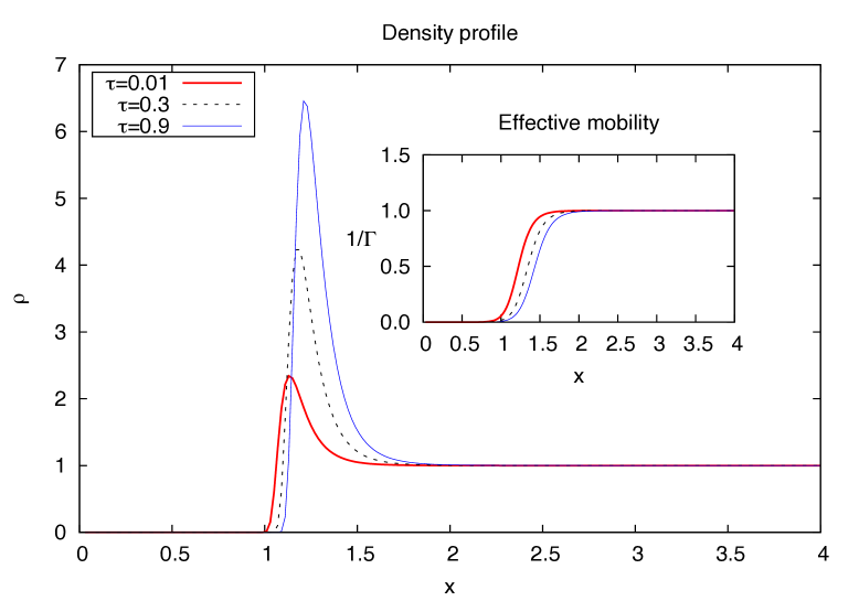
Figure 1: Three density profiles in the presence of a repulsive soft wall of the form $u(x)=u_{0}(\frac{\sigma}{x})^{12}$ corresponding to three different values of the persistence time $\tau$ as indicated in the box. In the inset we report the effective mobility profiles for the same values of $\tau$.

III.2 Interacting active particles and non ideal pressure via BGY equation

To extend eq.(15) to the case of interacting active particles we apply an external potential varying only in the direction $x$ and factorize the multiparticle distributions as $\rho^{(n)}({\bf r}_{1},\dots,{\bf r}_{n})\approx\rho^{(1)}({\bf r}_{1})\dots\rho^{(1)}({\bf r}_{n})$ invoking a mean field-like approximation and recast (14) as:

$$-T_{s}\frac{d}{dx_{1}}\left(\frac{\rho^{(1)}(x_{1})}{1+\frac{\tau}{\gamma}u_{x1,x1}(x_{1})+\frac{\tau}{\gamma}\int d{\bf r}_{2}\rho^{(1)}({\bf r}_{2})w_{x1,x1}({\bf r}_{1},{\bf r}_{2}))}\right)\approx$$

$$\rho^{(1)}(x_{1})\frac{d}{dx_{1}}u(x_{1})+\rho^{(1)}(x_{1})\int d{\bf r}_{2}\rho^{(1)}(x_{2})\frac{\partial}{\partial x_{1}}w({\bf r}_{1},{\bf r}_{2}))$$ (19)

where we have dropped off-diagonal terms $w_{\alpha\beta}$ in the denominator by the symmetry of the planar problem.

Formula (19) is valid up to linear order in $\tau/\gamma$ and in the l.h.s. contains the gradient of the density multiplied by a space dependent mobility, represented by the denominator. It generalizes to the interacting case the denominator featuring in formula (15) by the presence of inter-particle contributions. When $w_{xx}({\bf r})$ is positive it gives rise to a slowing down of particle motion due to the surrounding particles in interacting active systems and determines a density dependence of the mobility. In the r.h.s. the first two terms represent the external force term and the contribution to the pressure gradient due to direct "molecular" interactions, respectively. Notice again that the denominator represents the combined action of the "molecular" forces and the dynamics, and can be identified with the indirect interaction of Solon et al.. Eq. (19) in the limit $\tau\to 0$ reproduces the expression of the hydrostatic equilibrium of a standard molecular fluid in a local density approximation. There is an interesting analogy with granular gases subject to homogeneous shaking where the kinetic temperature can be a function of position and regions of higher density correspond to lower temperatures because the higher rate of inelastic collisions causes a higher energy dissipation rate Goldhirsch and Zanetti (1993); Marini-Bettolo-Marconi et al. (2007).

III.3 Effective pair potential

Equation (13) determines the pair correlation function of the model: $\rho^{(2)}({\bf r}_{1},{\bf r}_{2})=\bar{\rho}^{2}g(|{\bf r}_{1}-{\bf r}_{2}|)$ , but it suffers of the usual problem of statistical mechanics of liquids since it requires the knowledge of higher order correlations even at linear order in the expansion in the activity parameter. One could proceed further by assigning a prescription to determine the three particle correlation function $g_{3}$ in terms of $g(r)$ as done in the literature, but we shall not follow this approach and only consider the low density limit where it is possible to use it to derive a simple expression for $g(r)$ and define an effective interaction. In fact, the pair distribution function for a two particle system obtained from (9) reads:

$$g(r)=\exp\left(-\frac{w(r)+\frac{\tau}{\gamma}[(w^{\prime}(r)]^{2}-T_{s}\ln[(1+2\frac{\tau}{\gamma}w^{\prime\prime}(r))(1+2\frac{\tau}{\gamma}\frac{w^{\prime}(r)}{r})^{2}]}{T_{s}}\right)$$ (20)

where the apostrophes mean derivative with respect to the separation $r$. The effective pair potential is defined as $\phi(r)=-T_{s}\ln g(r)$. Let us remark that this method of introducing the effective potential does not account for the three body terms which instead would emerge from the solution of the BGY-like equation. The lack of such contributions affects the calculation of the virial terms beyond the second in the pressure equation of state discussed in section V.

IV Mean field pseudo-Helmholtz functional

As we have seen above, the BGY hierarchy is instructive, but unpractical because it requires a truncation scheme (for instance the Kirkwood superposition approximation at the level of two-particle distribution function to eliminate the three body distribution) and any progress can be obtained only numerically. The approximations involved are often difficult to assess, and for the sake of simplicity in the present paper we limit ourselves to a simpler mean field approach. A method often employed in equilibrium statistical mechanics to construct a mean field theory is the so called variational method based on the Gibbs-Bogoliubov inequality Hansen and McDonald (1990). At equilibrium one can prove that there exists a Helmholtz free energy functional, ${\cal F}^{eq}[f]$ of the probability density distribution, $f$, in configuration space such that it attains its minimum value, when the generic distribution $f$, selected among those which are normalized and non negative, corresponds to the equilibrium distribution function $f^{eq}$. Such a method can be generalized to the present non equilibrium case to develop a mean field theory. We start from the probability distribution (9) and introduce the "effective Helmholtz free energy" functional as

$${\cal F}[P_{N}^{trial}]\equiv\mathrm{Tr}P_{N}^{trial}({\cal H}+T_{s}\ln P_{N}^{trial})$$ (21)

where $\mathrm{Tr}\equiv\iint d{\bf r}_{1},\dots,d{\bf r}_{N}$ and $P_{N}^{trial}$ is an arbitrary $N$-particle normalized probability distribution, thus integrable and non negative. Define

$$Z_{N}=\mathrm{Tr}\exp\left[-\frac{{\cal H}({\bf r}_{1},\dots,{\bf r}_{N})}{T_{s}}\right].$$ (22)

The stationary probability distribution which minimizes ${\cal F}$ is:

$$f^{0}_{N}=\exp\left[-\frac{{\cal H}(x_{1},\dots,x_{N})}{T_{s}}\right]\,Z_{N}^{-1}$$ (23)

and is the analogue of the equilibrium density distribution. In fact, the effective free energy:

$${\cal F}_{0}[f^{0}_{N}]\equiv-T_{s}\ln Z_{N}[f^{0}_{N}]$$ (24)

is a lower bound for all distributions such that ${\cal F}[P^{trial}_{N}]>{\cal F}_{0}[f^{0}_{N}]$ for $P^{trial}_{N}\neq f^{0}_{N}$ (see ref. Hansen and McDonald (1990)).

In other words, the functional evaluated with any approximate distribution has a "free energy" higher than the one corresponding to the exact distribution. Since ${\cal F}$ is minimal at the steady state it is then reasonable to assume that it can play the role of an Helmholtz free energy in an equilibrium system. Using such an analogy we shall construct an explicit (but approximate) mean field expression of ${\cal F}$ in terms of the one body distribution function $P_{1}$ or equivalently $\rho^{(1)}$ Let us remark that our present results do not allow to establish the central achievement of density functional theory (DFT), namely the fact that the $N$-particle distribution function $f_{N}^{0}$ is a unique functional of the one body density distribution Evans (1979). This in turn means that for any fluid exposed to an arbitrary external potential $u({\bf r})$, the intrinsic free energy is a unique functional of equilibrium single-particle density .

Nevertheless, it is possible to prove another remarkable property of ${\cal F}$, an H-theorem, stating that the time derivative of ${\cal F}$ evaluated on a time dependent solution of the FPE is non positive, meaning that the functional always decreases during the dynamics and tends to a unique solution. The proof of this property is a simple application of a general result concerning the Fokker-Planck equation and can be found in the book by Risken Risken (1984) and in appendix B we provide the necessary elements to obtain it.

In order to construct the mean field approximation one assumes the following factorization of the $N$-particles probability distribution, $P^{trial}_{N}({\bf r}_{1},\dots,{\bf r}_{N})=\Pi_{k=1}^{N}P_{1}({\bf r}_{k})$, and minimizes the functional

$${\cal F}[P^{trial}_{N}]\equiv TrP^{trial}_{N}({\cal H}+T_{s}\ln P^{trial}_{N})$$ (25)

since the minimum of such a functional gives the closest value to the true functional ${\cal F}[f_{N}]$ within those having the product form as above:

$${\cal F}[P^{trial}_{N}]\equiv NT_{s}\int d{\bf r}P_{1}({\bf r})\ln P_{1}({\bf r})+TrP^{trial}_{N}{\cal H}\,$$ (26)

having used the fact that all $P_{1}$ are normalized to 1. Switching to the $\rho^{(1)}$ distribution we find:

$${\cal F}[\rho^{(1)}]=T_{s}\int d{\bf r}\rho^{(1)}({\bf r})(\ln\rho^{(1)}({\bf r})-1)+\sum_{1}^{N}\langle{\cal H}_{n}\rangle$$ (27)

where we considered the following decomposition of ${\cal H}=\sum_{1}^{N}{\cal H}_{n}$ into one body, two body, three body up to $N$-body interactions and their averages $\langle{\cal H}_{n}\rangle=\int\dots\int d{\bf r}_{1}\dots d{\bf r}_{n}\rho^{(1)}({\bf r}_{1})\dots\rho^{(1)}({\bf r}_{n}){\cal H}_{n}({\bf r},\dots,{\bf r}_{n}).$ The minimum of the functional ${\cal F}$ is obtained by differentiating w.r.t. to the $\rho^{(1)}({\bf r})$.

IV.1 Application to Planar and Spherical interfaces of non interacting systems

As an example we consider the "Helmholtz functional" for non interacting particles near a flat wall, for which only ${\cal H}_{1}$ contributes:

$${\cal F}[\rho^{(1)}]\propto\int dx\rho^{(1)}(x)\Bigl{(}T_{s}(\ln\frac{\rho^{(1)}(x)}{\rho_{0}}-1)-T_{s}\ln[1+\frac{\tau}{\gamma}u_{xx}(x)]+u(x)+\frac{\tau}{2\gamma}(u_{x}(x))^{2}\Bigl{)}$$ (28)

minimizing w.r.t. $\rho^{(1)}$ we obtain the same result as (16) which is exact. Similarly, the extension to three dimensional spherical walls is

$${\cal F}[\rho^{(1)}]=\int d{\bf r}\rho^{(1)}(r)\Bigl{(}T_{s}(\ln\frac{\rho^{(1)}(r)}{\rho_{0}}-1)-T_{s}\ln[(1+\frac{\tau}{\gamma}u^{\prime\prime}(r))(1+\frac{\tau}{\gamma}\frac{u^{\prime}(r)}{r})^{2}]+u(r)+\frac{\tau}{2\gamma}(u^{\prime}(r))^{2}\Bigl{)}$$

(29)

Notice the difference of order $\tau/\gamma$, namely a factor $2$, between the $g(r)$ found by considering two active particles and the single-particle density profile when a spherical wall particle is pinned at the origin. Such a non-equivalence is fingerprint of the off-equilibrium nature of the system and disappears as $\tau\to 0$.

IV.1.1 Mobility and pressure tensor in spherical symmetry

One can derive an interesting formula starting from (29). We first extremize the functional with respect to $\rho^{(1)}(r)$ (i.e. $\delta{\cal F}/\delta\rho^{(1)}(r)=0$ ) to obtain the profile, hence differentiate the result with respect to $r$ and multiply it by $\rho^{(1)}$ and arrive at the following formula:

$$T_{s}\frac{d}{dr}\left(\frac{\rho^{(1)}(r)}{1+\frac{\tau}{\gamma}u_{ext}^{\prime\prime}(r)}\right)+2\frac{T_{s}}{r}\left(\frac{\rho^{(1)}(r)}{1+\frac{\tau}{\gamma}u_{ext}^{\prime\prime}(r)}-\frac{\rho^{(1)}(r)}{1+\frac{\tau}{\gamma}u_{ext}^{\prime}(r)/r}\right)=-\rho^{(1)}(r)u_{ext}^{\prime}(r).$$ (30)

On the other hand in a system of spherical symmetry the pressure tensor, $p_{\alpha\beta}(r)$, at point ${\bf r}$ must be of the form: $p_{\alpha\beta}(r)=\hat{r}_{\alpha}\hat{r}_{\beta}p_{N}(r)+(\delta_{\alpha\beta}-\hat{r}_{\alpha}\hat{r}_{\beta})p_{T}(r)$, where we have separated the normal (N) and tangential (T) components and $\hat{\bf r}$ denotes unit vector in the radial direction. In the absence of currents the mechanical balance condition dictates

$$\frac{d}{dr}p_{N}(r)+\frac{2}{r}(p_{N}(r)-p_{T}(r))=-\rho^{(1)}(r)u_{ext}^{\prime}(r).$$

By comparing with eq. (30) we may identify the two components $p_{N}(r)=T_{s}\rho(r)/(1+\frac{\tau}{\gamma}u_{ext}^{\prime\prime}(r))$ and $p_{T}(r)=T_{s}\rho^{(1)}(r)/(1+\frac{\tau}{\gamma}u_{ext}^{\prime}(r)/r)$ Rowlinson and Widom (2013). It would be interesting to extend the above analysis to the case of interacting particles along the lines sketched in section III , but this task is left for a future paper. Eq. (30) provides an interesting generalization of the planar formula (15) to a spherical interface and shows that unlike equilibrium fluids the normal and tangential components of the pressure tensor of a gas of non interacting active particles are not equal in the proximity of a spherical wall, but they tend to the common value $T_{s}\rho^{(1)}$ when $\tau\to 0$ . Notice that $p_{T}(r)$ exceeds $p_{N}(r)$ for a repulsive wall-potential since $u_{ext}^{\prime}(r)<0$. By pursuing the analogy with equilibrium statistical mechanics one could identify the integral of the second term in eq. (30) with a mechanical surface tension, which by our argument would turn up to be negative in agreement with Bialké et al. Bialké et al. (2014). A question arises: what is the nature of $p_{N}$ and $p_{T}$? The two quantities are two components of the swim pressure tensor and are different from their common bulk value $p$, because near a a spherical obstacle the motilities of the particles along the normal and in the tangential plane to the surface are also different. As far as the mobility tensor is concerned in spherical geometry we can decompose it as

$$\frac{1}{\gamma}\Gamma^{-1}_{\alpha\beta}(r)=\frac{1}{\gamma}\left[\frac{1}{\Gamma_{N}(r)}\hat{r}_{\alpha}\hat{r}_{\beta}+\frac{1}{\Gamma_{T}(r)}(\delta_{\alpha\beta}-\hat{r}_{\alpha}\hat{r}_{\beta})\right]$$ (31)

with $\Gamma_{N}(r)=(1+\frac{\tau}{\gamma}u_{ext}^{\prime\prime}(r))$ and $\Gamma_{T}(r)=(1+\frac{\tau}{\gamma}u_{ext}^{\prime}(r)/r)$ which shows why the tangential motion is characterised by a higher mobility than the normal motion near a curved surface as reported by many authors on the basis of simulation results and phenomenological arguments Elgeti and Gompper (2013). Particles are free to slide along the directions tangential to the surface and this explains why $p_{T}>p_{N}$.

Recently, Smallenburg and Lowen Smallenburg and Löwen (2015) have studied numerically non interacting active spheres in spherical geometry and found that for finite curvature radii active particles in contact with the inside of the boundary tend to spend larger time than those at the outside and differences between the inner and the outer density profile as a function of the normal distance to the wall. To see how the density profile around a spherical repulsive wall reduces to the profile near a planar wall we use the explicit form of the solutions and introduce the normal distance, $z=r-R_{0}$, to the spherical wall defined by the potential $u_{0}\sigma^{n}/(r-R_{0})^{n}$ and write for $z>R_{0}$:

$$\rho^{(1)}(z)=\rho_{0}\exp\left[-\frac{1}{T_{s}}\left(u_{0}\left(\frac{\sigma}{z}\right)^{n}+\frac{\tau}{2\gamma}\frac{u_{0}^{2}}{\sigma^{2}}n^{2}\left(\frac{\sigma}{z}\right)^{2n+2}\right)\right]$$

$$\left(1+\frac{\tau}{\gamma}\frac{u_{0}}{\sigma^{2}}n(n+1)\left(\frac{\sigma}{z}\right)^{n+2}\right)\left(1-\frac{\tau}{\gamma}\frac{u_{0}}{\sigma}\frac{1}{R_{0}+z}n\left(\frac{\sigma}{z}\right)^{n+1}\right)^{2}.$$ (32)

In the limit of $z/R_{0}\to 0$ the spherical profile must reduce to the planar profile, and indeed this is the situation as one can see by expanding the formula above in powers of $z/R_{0}$ . For particles contained in a spherical cavity ($z<R_{0}$) the potential reads $u_{0}\sigma^{n}/(R_{0}-r)^{n}$ and one must replace the last factor by $\left(1+\frac{\tau}{\gamma}\frac{u_{0}}{\sigma}\frac{1}{R_{0}-z}n(\frac{\sigma}{z})^{n+1}\right)^{2}$. The average local density on the concave side of a sphere is larger than the corresponding density on the convex side as found numerically by Mallory et al. Mallory et al. (2014). This is illustrated in Fig. 2 and Fig. 3.

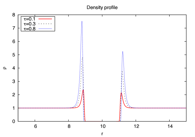
Figure 2: Comparison between the outer and the inner local density profiles for three choices of $\tau/\gamma$ in the presence of a repulsive spherical soft wall at $R_{0}=10$. Particles are non interacting.

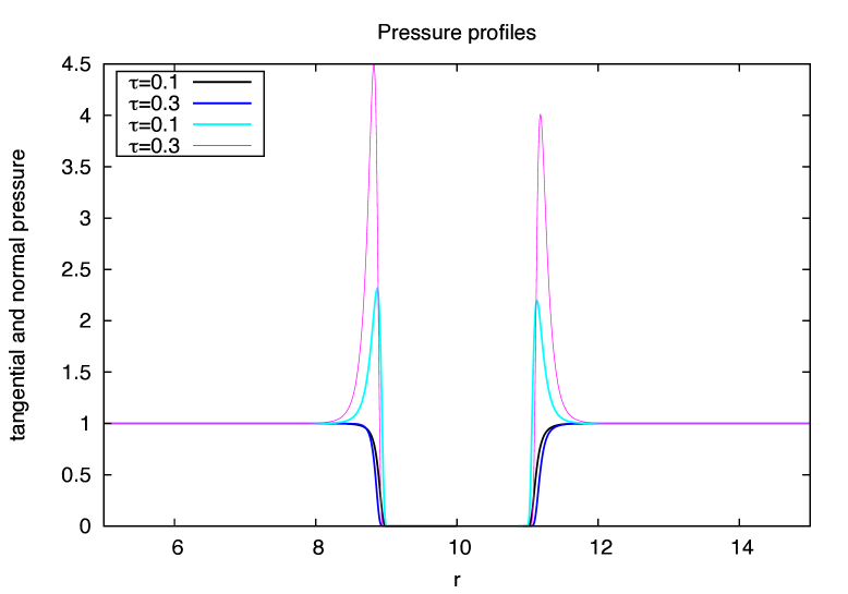
Figure 3: Comparison between the outer and the inner local pressures profiles for two choices of $\tau/\gamma$, 0.1 and 0.3 in the presence of a repulsive spherical soft wall at $R_{0}=10$. The tangential component displays a peak at a distance $\approx\sigma$ from the wall, whereas the normal component decreases monotonically as the wall is approached. Notice that the tangential components are always larger than the corresponding normal components.

IV.2 Can we write a density functional for interacting active particles?

As discussed above, since in the case of non interacting systems it is straightforward to construct an appropriate "Helmholtz" free energy functional such that it yields the same equation as the BGY method, one would like to determine the corresponding functional also in the case of interacting particles even within the simplest mean-field approximation. To this purpose we should construct a mean field functional ${\cal F}$ whose functional derivative with respect to $\rho^{(1)}$ gives a non equilibrium chemical potential $\mu(\rho^{(1)})$ whose gradient must vanish in the steady state giving a condition identical to the BGY equation (14). We have found that such a program can be carried out in the one dimensional case, in fact the following construction has the required properties

$${\cal F}[\rho^{(1)}]=T_{s}\int dx\rho^{(1)}(x)(\ln\frac{\rho^{(1)}(x)}{\rho_{0}}-1)-T_{s}\frac{\tau}{\gamma}\int dxu_{xx}(x)\rho^{(1)}(x)-\frac{1}{2}T_{s}\frac{\tau}{\gamma}\iint dxdx^{\prime}\,w_{xx}(x,x^{\prime})\rho^{(1)}(x)\rho^{(1)}(x^{\prime})$$

$$+\int dx\,u(x)\rho^{(1)}(x)+\frac{1}{2}\iint dxdx^{\prime}\,w(x,x^{\prime})\rho^{(1)}(x)\rho^{(1)}(x^{\prime})\,.$$ (33)

Unfortunately, we are not able to write the corresponding functional for dimensions higher than one, the difficulty being the presence of the off-diagonal elements of the friction matrix feauturing in eq. (14) which render the equation non integrable. In other words, eq. (14) is only a mechanical balance condition and involves transport coefficients, such as $\Gamma_{ij}$, thus revealing the true off-equilibrium nature of the active system, while in passive systems the transport coefficients never appear when thermodynamic equilibrium holds.

V Van der Waals bulk equation of state for active matter

As we have just seen the construction of a free energy functional capable of describing the inhomogeneous properties of active particles remains an open problem, nevertheless one can focus on the less ambitious task of determining the pseudo-free energy of a bulk system characterized by an effective pair interaction $\phi(r)$, defined in Section III. Notice that in the homogeneous case the friction matrix reduces to a scalar quantity due to the higher symmetry. As a prerequisite for a successful mean-field approximation $\phi(r)$ must be splitted into a short range repulsive part, $\phi_{rep}$, and a weaker longer range attractive contribution, $\phi_{at}$, and only the latter can be treated in a mean field fashion, since the effect of repulsion is a highly correlated phenomenon and not perturbative. Explicit expressions for the splitted potentials are given by (36) and (37). To capture the effect of repulsive forces a simple modification of the ideal gas entropic term, already introduced by van der Waals to account for the reduction of configurational entropy due to the finite volume of the particles, is sufficient. Thermodynamic perturbation theory would represent the natural choice to determine the total free energy. It assumes a reference hard-sphere system, whose Hamiltonian only depends on $\phi_{rep}$, as the unperturbed system. In particular the reference system characterized by a temperature dependent diameter, $d(T)$, allows to determine the free energy excess associated with the perturbing potential $\phi_{at}$ and and equation of state of the model. However, since perturbation theory still requires a considerable amount of computer calculations, here we make the simplest ansatz and write the following free energy functional

$${\cal F}_{vdW}=T_{s}\int dr\rho^{(1)}({\bf r})\left[\ln\left(\frac{\rho^{(1)}({\bf r})}{1-\frac{2\pi}{3}\rho^{(1)}({\bf r})d^{3}(T_{s})}\right)-1\right]+\frac{1}{2}\int d{\bf r}\int_{|{\bf r}^{\prime}-{\bf r}|>d}d{\bf r}^{\prime}\phi_{at}({\bf r}-{\bf r}^{\prime})\rho^{(1)}({\bf r})\rho^{(1)}({\bf r}^{\prime}).$$ (34)

The first term is just the entropy of a fluid with the excluded volume correction, the second term stems from the activity and may lead to condensation phenomena for large values of $\tau$. In relation to the naive mean-field functional (33), the van der Waals entropic term already contains the repulsive part of the direct interaction, whereas the attractive term which vanishes in the $\tau\to 0$ limit takes into account the activity. In principle this form of free energy can be constructed by employing the Mayer cluster expansion to evaluate $Z_{N}$, associated with the effective Hamiltonian ${\cal H}$, in the approximation of neglecting $m$-body interactions with $m>2$ there contained, that is using the effective potential $\phi(r)$. With these ingredients one can define the active component of the van der Waals attractive parameter:

$$a^{(A)}=-(1/2)\int_{r>d(T_{s})}d^{3}r\phi_{at}(r)$$ (35)

and the covolume

$$b=2\pi\frac{d^{3}(T_{s})}{3}$$

and estimate ${\cal F}_{vdW}$. Since the procedure adopted is completely analogous to the one employed in equilibrium fluids one can immediately derive a pressure equation by differentating ${\cal F}_{vdW}$ with respect to volume:

$$p_{vdW}=-\frac{\partial{{\cal F}_{vdW}}}{\partial V}=T_{s}\frac{\rho}{1-b\rho}-a^{(A)}\rho^{2}$$

which at low density reduces to the ideal bulk swim pressure $T_{s}\rho$. Going further, one can add a square gradient contribution to the free energy density, that simplifies the non local functional (34) while allowing to describe inhomogeneous systems. This is achieved by introducing a term $m|\nabla\rho|^{2}$, where $m=-(1/12)\int_{r>d(T_{s})}d^{3}rr^{2}\phi_{at}(r)$ Evans (1979). We choose, now, the bare potential of the form $w(r)=w_{0}(\frac{\sigma}{r})^{\alpha}$, where $w_{0}$ is the strength of the bare potential, $\sigma$ is a nominal diameter and define $\tilde{r}=r/\sigma$, the non dimensional temperature $T^{*}=\frac{T_{s}}{w_{0}}$ and the parameter $K_{p}=\frac{w_{0}\tau}{\gamma\sigma^{2}}=\frac{(1+D_{t}/D_{a})}{T^{*}}Pe^{2}$, where the last expression displays the dependence on the Péclet number. We, now, set :

$$\frac{\phi_{rep}(\tilde{r})}{T_{s}}=\frac{1}{T^{*}}\left(\frac{1}{\tilde{r}^{\alpha}}+K_{p}\frac{\alpha^{2}}{\tilde{r}^{2\alpha+2}}\right)$$ (36)

and

$$\frac{\phi_{at}(\tilde{r})}{T_{s}}=-\ln\left(\left[1+2K_{p}\frac{\alpha(\alpha+1)}{\tilde{r}^{\alpha+2}}\right]\left[1-2K_{p}\frac{\alpha}{\tilde{r}^{\alpha+1}}\right]^{2}\right)$$ (37)

for $\tilde{r}>1$. The effective hard-sphere diameter is given by the Barker-Henderson formula:

$$\frac{d(T_{s})}{\sigma}=\int_{0}^{\infty}d\tilde{r}(1-e^{-\phi_{rep}(\tilde{r})/T_{s}})$$ (38)

and is density independent, but depends on the parameter $K_{p}$ and temperature. As $K_{p}\to 0$ (i.e. at small Péclet number, i.e. small persistence time ) the system approaches the behavior of an assembly of passive soft spheres at temperature $T^{*}$, and inverse power law potentials analytic expressions for $d(T_{s})$ exist, whereas as $K_{p}\to\infty$ (large Péclet number) the activity becomes increasingly relevant and the effective radius increases with $K_{p}$.

Let us remark that with the definition (37) of attractive potential the coefficient $a^{(A)}$ of formula (35) has a strong dependence on the temperature $T_{s}$, at variance with standard passive fluids where the dependence occurs through $d(T_{s})$ only. This makes the condensation transition basically athermal and driven by the activity parameter. This feature renders the case of active particles possessing also a direct attractive potential contribution of the Lennard-Jones 6-12 type particularly interesting, that is obtained by modifying the bare pair potential as $w_{\lambda}(r)=w_{0}[(\frac{\sigma}{r})^{\alpha}-\lambda(\frac{\sigma}{r})^{\alpha/2}]$. In fact, one has to consider a passive contribution similar to (35) to the vdW coefficient, say $a^{(P)}$ whose dependence on temperature is rather weak as compared to $a^{(A)}$. Thus one can expect that at low temperature and small $Pe$ the condensation is driven by standard attraction, whereas at high $T_{s}$ but large $Pe$ the transition is determined by the effective attractive determined by the activity Redner et al. (2013).

We turn, now, to consider the virial series of the pressure:

$$\frac{p}{T_{s}\rho}=(1+B(\tau)\rho+C\rho^{2}+\dots)$$

and by comparing with the van der Waals equation we obtain second virial coefficient $B(\tau)=(\frac{2\pi}{3}\rho d^{3}-a^{(A)}(\tau)/T_{s})$. Using the effective pair potential we can obtain $B$ as the integral (with $\lambda=0$)

$$B(T^{*},K_{p})=2\pi\sigma^{3}\int_{0}^{\infty}d\tilde{r}\tilde{r}^{2}\Bigl{\{}1-\exp\Bigl{[}-\frac{1}{T^{*}}\Bigl{(}\frac{1}{r^{*\alpha}}+K_{p}\frac{\alpha^{2}}{\tilde{r}^{2\alpha+2}}\Bigl{)}\Bigl{]}$$

$$\left[1+2K_{p}\frac{\alpha(\alpha+1)}{\tilde{r}^{\alpha+2}}\right]\left[1-2K_{p}\frac{\alpha}{\tilde{r}^{\alpha+1}}\right]^{2}\Bigr{\}}.$$ (39)

Formula (39) gives the second virial coefficient for active spheres with purely repulsive potential a straightforward extension of it yields the values with finite values of $\lambda$.

The Boyle activity parameter, $\tau^{*}$ of the model, corresponds to the values where $B=0$. For systems without attraction the curve $T_{s}(\tau^{*})$ where $B(T_{s},\tau^{*})=0$ is monotonic and decreases when $\tau^{*}$ increases and the resulting phase diagram in a plane $\tau,T_{s}$ is shown in Fig 4: the region at the right of each line corresponds to $B<0$ for that given value of $\lambda$. The same calculation is repeated for an active system with attraction and we found that the locus where $B(T_{s},\tau^{*})=0$ initially decreases as a function of $\tau$, but then it bends as displayed in Fig. 4 and shows at sufficiently low temperatures $T_{s}$ shows the presence of a region close to the origin where $B<0$. Figure 4 displays a reentrant behavior of the Boyle’s line for $\alpha=12$ when $\lambda>0$: at low temperatures $T^{*}$ the region $B<0$ under the effect of the direct attractive force extends at small values of $\tau$, while the bending is totally absent in the case $\lambda=0$. The Barker-Henderson diameter diplays the same non monotonic trend along the Boyle line showing the correlation between the structural properties and the thermal properties of the system.

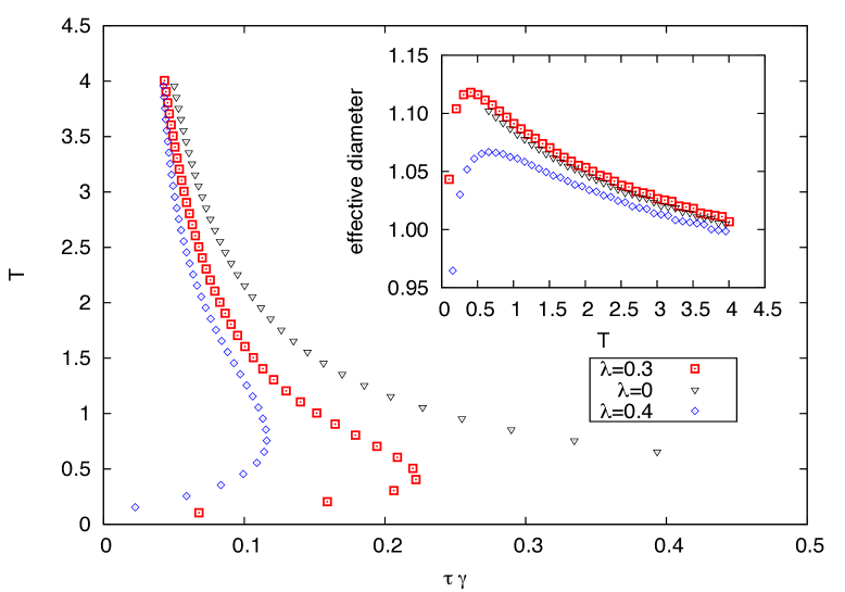
Figure 4: Plane $\tau,T_{s}$: the three curves in the main panel correspond to three different values (from right to left) of the attractive parameter $\lambda=0,0.2,0.4$ and $\alpha=12$, respectively, and represent the loci where the second virial coefficient, $B(\tau,T_{s})$, vanishes. In the purely repulsive case (triangles) the behavior is monotonic, whereas when attraction is present the lines bend in the low temperature region, where B changes sign under the effect of the direct attractive force. In the inset we plot the effective Barker-Henderson diameter as a function of the effective temperature measured along the Boyle line in the three cases.

VI Conclusions

In this paper we have investigated using a microscopic approach the steady state properties of a system of active particles and determined the stationary $N$-particle probability distribution function by requiring the vanishing of all currents. We used such a distribution to construct the BGY hierarchy for the reduce $n$-particle (with $n<N$) distribution functions and found that it contains terms which do not have a counterpart in systems of passive particles. The presence of these terms explains several experimental or numerical findings such the modified barometric law, the effective attraction between nominally repulsive objects, negative second virial coefficient, condensation. We defined an effective potential of attractive character due to the reduced mobility experienced by the active particles and determined by the combined effect of the excluded volume and the persistence of their motion. In an inhomogeneous environment the mobility turns out to be anisotropic and described by a tensor, whose expression we have obtained in the case of a spherical surface by separating its normal and tangential components. The same type of analysis allows to determine the mechanical pressure in systems of non interacting active particles via an hydrostatic balance, but the full extension to the interacting case remains an open problem. In order to obtain a bulk equation of state connecting pressure to density, swim temperature and activity parameter we have explored an alternative approach and constructed a mean field theory introducing a (pseudo) Helmholtz functional and determined the stationary distribution by a variational principle. In spite of the great similarities with equilibrium systems, profound differences remain. Already at the level of the first BGY equation one sees that it is not possible to disentangle the interaction terms stemming from the external potential from those from the particle-particle interactions. Such a feature in our opinion seems to obstruct the way to establish a full density functional theory. In fact, it does not seem possible to prove the so called v-representability property, i.e. the unique correspondence between the one particle density profile and a given external potential, which is at the basis of DFT. On the hand, if one constructs the functional using the two body effective potential $\phi(r)$ the DFT approach sounds promising to tackle the properties of active particles under inhomogeneous condition. Finally we note that the homogeneous free energy that we have constructed seems to reproduce the behaviour of the active fluid, helps in locating its instabilities and the onset of phase separation. In this context it would be very interesting to compare our approximate theory with numerical simulations of interacting colored-noise driven particles. In the future we plan to apply the pseudo-Helmholtz functional to the analysis of strongly in-homogeneous systems of active particles and to investigate the MIPS in these situations.

Appendix A Multidimensional unified colored noise approximation

In the present appendix, following the method put forward by Cao and coworkers Cao et al. (1993); Ke et al. (1999), we introduce an auxiliary stochastic process, $w_{i}$, defined by:

$$w_{i}=\frac{F_{i}}{\gamma}+v_{i}.$$

By taking the derivative of $w_{i}$ with respect to $t$ we obtain

$$\dot{w}_{i}=\frac{1}{\gamma}\sum_{k}\frac{\partial F_{i}}{\partial x_{k}}\dot{x}_{k}+\dot{v}_{i}.$$ (40)

after substituting into eq. (40) relations (1)and (2) to eliminate $\dot{v}_{i}$ and $\dot{x}_{k}$ we arrive at the evolution equation for $w_{i}$:

$$\dot{w}_{i}=\frac{1}{\gamma}\sum_{k}\frac{\partial F_{i}}{\partial x_{k}}(w_{k}+D_{t}^{1/2}\xi^{t}_{k})-\frac{1}{\tau}\left[w_{i}-\frac{F_{i}}{\gamma}\right]+\frac{D_{a}^{1/2}}{\tau}\eta_{i}(t).$$ (41)

Now, we assume the unified colored noise approximation (UCNA) Hanggi and Jung (1995) consisting in dropping the "acceleration term", $\dot{w}_{i}$, featuring in the l.h.s. of this equation, so that we can write the following system of algebraic linear equations for the quantities $w_{i}$:

$$\left[\delta_{ik}-\frac{\tau}{\gamma}\sum_{k}\frac{\partial F_{i}}{\partial x_{k}}\right]w_{k}=\frac{\tau}{\gamma}\sum_{k}\frac{\partial F_{i}}{\partial x_{k}}D_{t}^{1/2}\xi^{t}_{k}+\frac{F_{i}}{\gamma}+D_{a}^{1/2}\eta_{i}(t).$$ (42)

With the help of the matrix $\Gamma_{ik}$ (defined by eq.(4)) we go back to the equation for $x_{i}$ eq.(1) , rewritten as $w_{i}=\dot{x}_{i}-D_{t}^{1/2}\xi_{i}^{t}$, to find the following Langevin equation:

$$\dot{x}_{i}\simeq\sum_{k}\Gamma^{-1}_{ik}\frac{1}{\gamma}F_{k}+D_{a}^{1/2}\Gamma^{-1}_{ik}\eta_{k}(t)+D_{t}^{1/2}\xi^{t}_{i}(t)+D_{t}^{1/2}\frac{\tau}{\gamma}\sum_{k}\Gamma^{-1}_{ik}\sum_{l}\frac{\partial F_{k}}{\partial x_{l}}\xi^{t}_{l}$$ (43)

that we interpret using the Stratonovich convention Gardiner (1985). We finally observe that the last two terms can be gathered together and after some manipulations reported hereafter

$$\sum_{l}\Bigl{[}\delta_{il}+\sum_{k}\Gamma^{-1}_{ik}\frac{\tau}{\gamma}\frac{\partial F_{k}}{\partial x_{l}}\Bigl{]}\xi^{t}_{l}=\sum_{l}\sum_{k}\Bigl{[}\Gamma^{-1}_{ik}\Gamma_{kl}+\Gamma^{-1}_{ik}\frac{\tau}{\gamma}\frac{\partial F_{k}}{\partial x_{l}}\Bigl{]}\xi^{t}_{l}=$$

$$=\sum_{l}\sum_{k}\Gamma^{-1}_{ik}\Bigl{[}\Gamma_{kl}+\frac{\tau}{\gamma}\frac{\partial F_{k}}{\partial x_{l}}\Bigl{]}\xi^{t}_{l}=\sum_{l}\sum_{k}\Gamma^{-1}_{ik}\delta_{kl}\xi^{t}_{l}=\sum_{k}\Gamma^{-1}_{ik}\xi^{t}_{k}$$

give rise to the form of the stochastic equation for $x_{i}$ reported in eq.(3).

We limit ourselves to consider the stationary solutions with vanishing current and since we have assumed that the determinant is non vanishing the only solution of eq. (6) corresponding to $J_{l}=0$ is obtained by imposing the conditions:

$$\frac{1}{(D_{a}+D_{t})\gamma}F_{k}P_{N}-P_{N}\sum_{j}\frac{\partial}{\partial x_{j}}\Gamma^{-1}_{jk}=\sum_{j}\Gamma^{-1}_{jk}\frac{\partial}{\partial x_{j}}P_{N}$$ (44)

Multiplying by $\Gamma_{nk}$ and summing over $k$ after some algebra we obtain the first order differential equations for $P_{N}$:

$$P_{N}\frac{\tau}{(D_{a}+D_{t})\gamma}\sum_{k}\Gamma_{nk}F_{k}+P_{N}\sum_{jk}\Gamma^{-1}_{jk}\left(\frac{\partial}{\partial x_{j}}\Gamma_{kn}\right)=\frac{\partial P_{N}}{\partial x_{n}}$$ (45)

Since the matrix elements $\Gamma_{ij}$ contain 2-nd cross derivatives $\partial^{2}/\partial x_{i}\partial x_{j}$ of the potential ${\cal U}$ we have

$$\frac{\partial}{\partial x_{j}}\Gamma_{kn}=\frac{\partial}{\partial x_{n}}\Gamma_{kj}$$ (46)

and we finally get

$$\sum_{jk}\Gamma^{-1}_{jk}\left(\frac{\partial}{\partial x_{j}}\Gamma_{kn}\right)=\sum_{jk}\Gamma^{-1}_{jk}\left(\frac{\partial}{\partial x_{n}}\Gamma_{kj}\right)=\frac{1}{\det\Gamma}\frac{\partial}{\partial x_{n}}\det\Gamma$$ (47)

The last equality derives from the following Jacobi’s formula

$$\frac{1}{\det\Gamma}\frac{\partial}{\partial y}\det\Gamma=\mathrm{Tr}\left(\Gamma^{-1}\frac{\partial}{\partial y}\Gamma\right)$$ (48)

where $y$ stands for any of the variables $x_{i}$.

Explicitly by using (45) and (47) we find the system of differential equations (7) determining the full probability distribution.

Appendix B H-theorem for the FPE

The functional ${\cal F}[f_{N}]=Trf_{N}({\cal H}+T_{s}\ln f_{N})$ discussed in Sect. IV has also an interesting dynamical property. In fact, after rewriting it under the form

$$\frac{1}{T_{s}}{\cal F}[f_{N}]=Trf_{N}\ln\left(\frac{f_{N}}{P_{N}}\right)-\ln Z_{N}$$

where $f_{N}(\{x\},t)$ is a normalized solution of the dynamical Fokker-Planck equation at instant $t$ and $P_{N}$ is the stationary distribution and the first term is the so called Kullback-Leibler relative entropy Risken (1984); Kullback and Leibler (1951). One can show the following H-theorem

$$\frac{d{\cal F}}{dt}\leq 0.$$ (49)

The proof follows closely the method presented by Risken Risken (1984) (section 6.1 of his book), but before proceeding it is necessary to reduce the FPE described by eqs. (5) and (6) to the canonical form:

$$\frac{\partial f_{N}}{\partial t}=\sum_{i}\frac{\partial}{\partial x_{i}}\Bigl{[}\sum_{j}\frac{\partial}{\partial x_{j}}D_{ij}^{(2)}f_{N}-D_{i}^{(1)}f_{N}\Bigr{]}$$ (50)

where the diffusion matrix is

$$D_{ij}^{(2)}=(D_{a}+D_{t})\,\Gamma^{-2}_{ij}$$ (51)

and the drift vector is

$$D_{i}^{(1)}=\frac{1}{\gamma}\Gamma^{-1}_{lk}\,F_{k}+(D_{a}+D_{t})\Gamma^{-1}_{jk}\,\frac{\partial}{\partial x_{j}}\Gamma^{-1}_{ik}$$ (52)

Now using some standard analytic manipulations reported by Risken it is simple to show the following formula

$$\frac{d{\cal F}}{dt}=-\int d^{N}xf_{N}D_{ij}^{(2)}\,\frac{\partial\ln R}{\partial x_{i}}\frac{\partial\ln R}{\partial x_{j}}\leq 0$$ (53)

where $R=f_{N}/P_{N}$. If $D_{ij}^{(2)}$ is positive definite ${\cal F}$ must always decrease for $\frac{\partial\ln R}{\partial x_{i}}\neq 0$ towards the minimum value $-T_{s}\ln Z_{N}$. This result also implies that the solution of the FPE is unique, and after some time T the distance between two solutions is vanishingly small.

Appendix C Detailed Balance

The detailed balance implies a stronger condition than the one represented by having a stationary distribution, since it implies that there is no net flow of probability around any closed cycle of states. In practice if detailed balance holds it is not possible to have a ratchet mechanism and directed motion. Again we use the equations derived by Risken (Section 6.4 of his book)Risken (1984) which represent the sufficient and necessary conditions for detailed balance. Since the variables $\{x_{i}\}$ are even under time reversal we have to verify the validity of the following equations Van Kampen (1957); Graham and Haken (1971):

$$D_{i}^{(1)}\,P_{N}(\{x\})=\frac{\partial}{\partial x_{j}}D_{ij}^{(2)}\,P_{N}(\{x\})$$ (54)

Using the explicit form of (51) and (52) it is straightforward to verify that the detailed balance conditions are verified since they are the same as the condition expressing the vanishing of the current components $J_{i}$ in the stationary state (see eq. (50).

Appendix D Approximation for the determinant

The exact evaluation of the determinant $\Gamma$ associated with the Hessian matrix is beyond the authors capabilities and we look for approximations in order to evaluate the effective forces. We consider the associated determinant in the case of two spatial dimensions:

$$\small\left(\begin{array}[]{ccccccc}[1+\frac{\tau}{\gamma}\sum_{j\neq 1}w_{xx}({\bf r}_{1},{\bf r}_{j})]&\sum_{j\neq 1}\frac{\tau}{\gamma}w_{xy}({\bf r}_{1},{\bf r}_{j})&-\frac{\tau}{\gamma}w_{xx}({\bf r}_{1},{\bf r}_{2})&\dots&-\frac{\tau}{\gamma}w_{xy}({\bf r}_{1},{\bf r}_{N})\\ \sum_{j\neq 1}\frac{\tau}{\gamma}w_{yx}({\bf r}_{1},{\bf r}_{j})&[1+\frac{\tau}{\gamma}\sum_{j\neq 1}w_{yy}({\bf r}_{1},{\bf r}_{j})]&-\frac{\tau}{\gamma}w_{yx}({\bf r}_{1},{\bf r}_{2})&\dots&-\frac{\tau}{\gamma}w_{yy}({\bf r}_{1},{\bf r}_{N})\\ -\frac{\tau}{\gamma}w_{xx}({\bf r}_{2},{\bf r}_{1})&-\frac{\tau}{\gamma}w_{yx}({\bf r}_{2},{\bf r}_{1})&[1+\frac{\tau}{\gamma}\sum_{j\neq 2}w_{xx}({\bf r}_{2},{\bf r}_{j})]&\dots&-\frac{\tau}{\gamma}w_{xy}({\bf r}_{2},{\bf r}_{N})\\ \\ \dots&\dots&\dots&\dots&\dots&\\ \\ -\frac{\tau}{\gamma}w_{xy}({\bf r}_{N},{\bf r}_{1})&-\frac{\tau}{\gamma}w_{yy}({\bf r}_{N},{\bf r}_{1})&\dots&\dots&[1+\frac{\tau}{\gamma}\sum_{j\neq N}w_{yy}({\bf r}_{N},{\bf r}_{j})]\end{array}\right)$$

and to order $\tau/\gamma$ is

$$\det\Gamma\approx 1+\frac{\tau}{\gamma}\sum_{i,j,i\neq j}[w_{xx}({\bf r}_{i},{\bf r}_{j})+w_{yy}({\bf r}_{i},{\bf r}_{j})]$$ (55)

It is interesting to remark that the off-diagonal elements contain only one term, while the diagonal elements and their neighbors contain $N$ elements. Thus in the limit of $N\to\infty$ we expect that the matrix becomes effectively diagonal.

References

- Romanczuk et al. (2012) P. Romanczuk, M. Bär, W. Ebeling, B. Lindner, and L. Schimansky-Geier, The European Physical Journal Special Topics 202, 1 (2012).
- Elgeti et al. (2014) J. Elgeti, R. G. Winkler, and G. Gompper, arXiv preprint arXiv:1412.2692 (2014).
- Marchetti et al. (2013) M. Marchetti, J. Joanny, S. Ramaswamy, T. Liverpool, J. Prost, M. Rao, and R. A. Simha, Reviews of Modern Physics 85, 1143 (2013).
- Ramaswamy (2010) S. Ramaswamy, The Mechanics and Statistics of Active Matter 1, 323 (2010).
- Berg (2004) H. C. Berg, E. coli in Motion (Springer Science & Business Media, 2004).
- Schnitzer (1993) M. J. Schnitzer, Physical Review E 48, 2553 (1993).
- Tailleur and Cates (2008) J. Tailleur and M. Cates, Physical review letters 100, 218103 (2008).
- Valeriani et al. (2011) C. Valeriani, M. Li, J. Novosel, J. Arlt, and D. Marenduzzo, Soft Matter 7, 5228 (2011).
- Di Leonardo et al. (2010) R. Di Leonardo, L. Angelani, D. Dell?Arciprete, G. Ruocco, V. Iebba, S. Schippa, M. Conte, F. Mecarini, F. De Angelis, and E. Di Fabrizio, Proceedings of the National Academy of Sciences 107, 9541 (2010).
- Schwarz-Linek et al. (2012) J. Schwarz-Linek, C. Valeriani, A. Cacciuto, M. Cates, D. Marenduzzo, A. Morozov, and W. Poon, Proceedings of the National Academy of Sciences 109, 4052 (2012).
- Poon (2013) W. Poon, Proceedings of the International School of Physics Enrico Ferm, Course CLXXXIV Physics of Complex Colloids, eds. C. Bechinger, F. Sciortino and P. Ziherl, IOS, Amsterdam: SIF, Bologna pp. 317–386 (2013).
- Cates (2012) M. Cates, Reports on Progress in Physics 75, 042601 (2012).
- Bialké et al. (2014) J. Bialké, H. Löwen, and T. Speck, arXiv preprint arXiv:1412.4601 (2014).
- Smallenburg and Löwen (2015) F. Smallenburg and H. Löwen, arXiv preprint arXiv:1504.05080 (2015).
- Baskaran and Marchetti (2010) A. Baskaran and M. C. Marchetti, Journal of Statistical Mechanics: Theory and Experiment 2010, P04019 (2010).
- Fily and Marchetti (2012) Y. Fily and M. C. Marchetti, Physical review letters 108, 235702 (2012).
- Stenhammar et al. (2013) J. Stenhammar, A. Tiribocchi, R. J. Allen, D. Marenduzzo, and M. E. Cates, Physical review letters 111, 145702 (2013).
- Takatori and Brady (2014) S. C. Takatori and J. F. Brady, arXiv preprint arXiv:1411.5776 (2014).
- Koumakis et al. (2014) N. Koumakis, C. Maggi, and R. Di Leonardo, Soft matter 10, 5695 (2014).
- Maggi et al. (2014) C. Maggi, M. Paoluzzi, N. Pellicciotta, A. Lepore, L. Angelani, and R. Di Leonardo, Physical review letters 113, 238303 (2014).
- Maggi et al. (2015) C. Maggi, U. M. B. Marconi, N. Gnan, and R. Di Leonardo, Scientific Reports 5 (2015).
- Farage et al. (2015) T. Farage, P. Krinninger, and J. Brader, Physical Review E 91, 042310 (2015).
- Angelani et al. (2011) L. Angelani, C. Maggi, M. Bernardini, A. Rizzo, and R. Di Leonardo, Physical review letters 107, 138302 (2011).
- Cates and Tailleur (2014) M. E. Cates and J. Tailleur, arXiv preprint arXiv:1406.3533 (2014).
- Hanggi and Jung (1995) P. Hanggi and P. Jung, Advances in Chemical Physics 89, 239 (1995).
- Lindner et al. (1999) B. Lindner, L. Schimansky-Geier, P. Reimann, P. Hänggi, and M. Nagaoka, Physical Review E 59, 1417 (1999).
- Gardiner (1985) C. Gardiner, Stochastic methods (Springer-Verlag, Berlin–Heidelberg–New York–Tokyo, 1985).
- Marconi and Tarazona (2006) U. M. B. Marconi and P. Tarazona, The Journal of Chemical Physics 124, 164901 (2006).
- Takatori et al. (2014) S. Takatori, W. Yan, and J. Brady, Physical review letters 113, 028103 (2014).
- Solon et al. (2015a) A. Solon, Y. Fily, A. Baskaran, M. Cates, Y. Kafri, M. Kardar, and J. Tailleur, Nature Physics (2015a).
- Solon et al. (2015b) A. P. Solon, J. Stenhammar, R. Wittkowski, M. Kardar, Y. Kafri, M. E. Cates, and J. Tailleur, Physical Review Letters 114, 198301 (2015b).
- Winkler et al. (2015) R. G. Winkler, A. Wysocki, and G. Gompper, Soft matter 11, 6680 (2015).
- Tailleur and Cates (2009) J. Tailleur and M. Cates, EPL (Europhysics Letters) 86, 60002 (2009).
- Palacci et al. (2010) J. Palacci, C. Cottin-Bizonne, C. Ybert, and L. Bocquet, Physical Review Letters 105, 088304 (2010).
- Maggi et al. (2013) C. Maggi, A. Lepore, J. Solari, A. Rizzo, and R. Di Leonardo, Soft Matter 9, 10885 (2013).
- Goldhirsch and Zanetti (1993) I. Goldhirsch and G. Zanetti, Physical review letters 70, 1619 (1993).
- Marini-Bettolo-Marconi et al. (2007) U. Marini-Bettolo-Marconi, P. Tarazona, and F. Cecconi, The Journal of Chemical Physics 126, 164904 (2007).
- Hansen and McDonald (1990) J.-P. Hansen and I. R. McDonald, Theory of simple liquids (Elsevier, 1990).
- Evans (1979) R. Evans, Advances in Physics 28, 143 (1979).
- Risken (1984) H. Risken, Fokker-Planck Equation (Springer, 1984).
- Rowlinson and Widom (2013) J. S. Rowlinson and B. Widom, Molecular theory of capillarity (Courier Corporation, 2013).
- Elgeti and Gompper (2013) J. Elgeti and G. Gompper, EPL (Europhysics Letters) 101, 48003 (2013).
- Mallory et al. (2014) S. Mallory, C. Valeriani, and A. Cacciuto, Physical Review E 90, 032309 (2014).
- Redner et al. (2013) G. S. Redner, A. Baskaran, and M. F. Hagan, Physical Review E 88, 012305 (2013).
- Cao et al. (1993) L. Cao, D.-j. Wu, and X.-l. Luo, Physical Review A 47, 57 (1993).
- Ke et al. (1999) S. Ke, D. Wu, and L. Cao, The European Physical Journal B-Condensed Matter and Complex Systems 12, 119 (1999).
- Kullback and Leibler (1951) S. Kullback and R. A. Leibler, The annals of mathematical statistics pp. 79–86 (1951).
- Van Kampen (1957) N. Van Kampen, Physica 23, 707 (1957).
- Graham and Haken (1971) R. Graham and H. Haken, Zeitschrift für Physik 243, 289 (1971).