Diffractive Electromagnetic Processes from a Regge Point of View

Abstract

The energy dependence of the cross sections for electromagnetic diffractive processes can be well described by a single power, $W^{\delta}$. For $J/\psi$ photoproduction this holds in the range from 20 GeV to 2 TeV. This feature is most easily explained by a single pole in the angular momentum plane which depends on the scale of the process, at least in a certain range of values of the momentum transfer. It is shown that this assumption allows a unified description of all electromagnetic elastic diffractive processes. We also discuss an alternative model with an energy dependent dipole cross section, which is compatible with the data up to 2 TeV and which shows an energy behaviour typical for a cut in the angular momentum plane.

I Introduction

Diffractive processes involving virtual photons show a remarkable feature: the higher the photon virtuality $Q^{2}$, the faster is the increase of the cross sections with energy. This feature is well understood in perturbative QCD, where the evolution equations in $Q^{2}$ Gribov:1972ri ; Altarelli:1977zs ; Dokshitzer:1977sg predict such a behaviour; the rising rate of increase in energy can be traced back to the increase of the gluon density with higher resolution.

This specific feature of the energy dependence, however, is less easily explained in Regge theory Col77 . The underlying core concept of this theory is the Sommerfeld-Watson transform Wat19 ; Som49 . The sum over the partial waves of a scattering amplitude in the $t$ channel is replaced by a contour integral in the angular momentum plane. The high energy behaviour of a process in the $s$ channel is determined by the position of the singularity in the complex angular momentum plane farthest to the right. If the singularity is a pole at position $\ell=\alpha$ the high energy behaviour of the amplitude is ${\cal T}\sim(W/W_{0})^{2\alpha}$. If it is a branch cut at $\ell=\alpha_{C}$ the power behaviour, up to logarithmic terms, is ultimately driven to ${\cal T}\sim(W/W_{0})^{2\alpha_{c}}$, but the explicit form depends crucially on the behaviour of the discontinuity across the cut.

Usually the positions of the singularities in the complex plane are assumed to be independent of the specific process. In purely hadronic diffractive processes the energy dependence of the scattering amplitude is supposed to be determined by the position $\alpha_{\bf P}(t)$ of a specific singularity, the “Pomeron trajectory” which depends on the squared momentum transfer $t$. Based on a large amount of hadronic diffractive data, Donnachie and Landshoff Donnachie:1992ny proposed a general description with $\alpha_{\bf P}(0)\approx 1.09$ and a slope ${d\alpha_{\bf P}}/{dt}=\alpha_{\bf P}^{\prime}=0.25\nobreak\,\mbox{GeV}^{-2}$.

On the other hand, by summing up leading-log terms in perturbative QCD, a Pomeron with a larger value $\alpha_{P}(0)$ was found (BFKL-Pomeron) Fadin:1975cb ; Kuraev:1977fs ; Balitsky:1978ic ; Ciafaloni:1998gs ; Fadin:1998py . Donnachie and Landshoff Donnachie:1998gm extended the Pomeron concept and assumed that electromagnetic diffractive processes are determined by two Pomerons, a soft (hypercritical) one with $\alpha_{\bf P}(0)=1.09$ and a hard one with a value of 1.42. This idea has been applied in many electroproduction processes, where the couplings to the two Pomerons were essentially determined by the size of the scattered objects and hence in a given model the energy dependence was universally fixed by a superposition of the two Pomeron contributions. In this way a comprehensive description of proton structure functions, vector meson production and $\gamma^{*}$-$\gamma^{*}$ scattering could be achieved in the full energy range accessible at HERA Dosch:1994ym ; Dosch:1997nw ; Kulzinger:1998hw ; Donnachie:1999kp ; Donnachie:2000px ; Donnachie:2001wt ; Dosch:2002ig ; Dosch:2006kz ; Baltar:2009vp .

Recent experiments of $J/\psi$ photoproduction at LHC at energies up to the TeV region LHCb(14) ; Alice(14) have shown, however, that a single power, corresponding to $\alpha_{\bf P}(0)=1.17$ describes very well the energy dependence in the range from 20 GeV to 2 TeV. This behaviour, although with larger experimental uncertainties, has also been found in $\Upsilon$ photoproduction LHCb(15) . These results are hardly compatible with the two Pomeron picture and rather support the concept of a single singularity in the angular momentum plane determining the high energy behaviour.

Our paper is organized as follows. In Sect. II we discuss the possibility of scale-dependent singularities in the complex angular momentum plane and define scales which allow to relate the energy dependence of vector meson production cross sections to the $x$-dependence of the proton structure function. In Sect. III we consider a model for $\gamma^{*}\,p$ scattering and diffractive vector meson production where the energy dependence is due to a specific energy dependence of the dipole cross section. In Sect. IV we compare the results of both models with experiment. Finally in Sect. V we compare the two approaches and discuss the implications on the Regge picture.

This paper is an extension of our earlier preprint Scale-Dependent Pomeron Intercept in Electromagnetic Diffractive Processes, arXiv:1503.06649 [hep-ph], and replaces it.

II Scale-dependent Regge singularities

II.1 General considerations

We sketch essential features of the Sommerfeld-Watson transform, neglecting details needed to include spin and signature effects. We consider the reaction visualized in Fig. 1, involving a virtual photon $\gamma^{*}$, two protons $p$ and a particle $X$ with the same quantum numbers as $\gamma^{*}$; the latter can be either be a virtual photon or a vector meson.

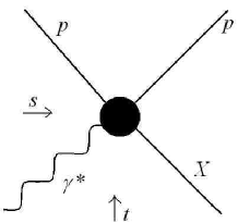
Figure 1: Virtual photon scattering ($X=\gamma^{*}$) or diffractive vector meson electroproduction ($X$ denotes a vector meson) off protons.

In an obvious notation we denote by $p_{\gamma^{*}},\,p_{p},\,p_{X}$ the momentum of the virtual photon, the incoming proton, and the particle $X$, respectively; $Q^{2}=-p_{\gamma^{*}}^{2}$ is the photon virtuality, $m_{p}$ the proton mass and $m_{X}^{2}=p_{X}^{2}$ . The squared CM energy and momentum transfer in the $s$ channel are $s=(p_{\gamma^{*}}+p_{p})^{2},\;t=(p_{X}-p_{\gamma^{*}})^{2}$; ${\cal T}(Q^{2},s,t)$ is the scattering amplitude involving these particles. In the $s$ channel the amplitude ${\cal T}(Q^{2},s,t)$ describes the process $\gamma^{*}\,p\to X\,p$, in the $t$ channel it describes the process $\gamma^{*}\,\bar{X}\to p\bar{p}$.

The partial wave representation of this amplitude in the $t$ channel is given by

$${\cal T}(Q^{2},s,t)=\sum_{\ell}(2\ell+1)~{}{\cal T}_{\ell}(Q^{2},t)~{}P_{\ell}(z_{t})~{},$$ (1)

where $z_{t}$ is the cosine of the CM scattering angle in this channel,

$$z_{t}=\frac{\sqrt{t}\;(2s+t-2m_{p}^{2}-m_{X}^{2}+Q^{2})}{\sqrt{\big{(}t^{2}-2t(m_{X}^{2}-Q^{2})+(m_{X}^{2}+Q^{2})\big{)}\,\big{(}t-4m_{p}^{2}\big{)}}}~{}.$$ (2)

By the Sommerfeld-Watson transformation the sum in Eq. (1) is expressed as the contour integral

$${\cal T}(Q^{2},s,t)=\int_{C}d\ell\,(2\ell+1)~{}{\cal T}_{\ell}(Q^{2},t)~{}\frac{P_{\ell}(z_{t})}{\sin\pi\ell}~{}.$$ (3)

Since for large $s$ and fixed $t$ and $Q^{2}$ the quantities $z_{t}$ and $P_{\ell}(z)$ behave like $z_{t}\sim s$ and $P_{\ell}(z)\sim z^{\ell}$, the high energy behaviour of ${\cal T}$ is determined by the position of the singularity in the $\ell$ plane with the largest value of $\Re\ell$. If this singularity is a pole at position $\ell=\alpha_{\bf P}(Q^{2},t)$ then the high energy behaviour is

$${\cal T}(Q^{2},s,t)\sim s^{\alpha_{\bf P}(Q^{2},t)}~{},$$ (4)

and in electromagnetic diffractive processes its position has to depend on the photon virtuality $Q^{2}$ in order to be compatible with the data as described above. Therefore the assumption of a universal position of the singularities in the complex angular momentum plane for all virtualities has to be abandoned in this case. This does not preclude the possibility that in the $t$ channel, $t>0$, there might exist hadrons corresponding to the poles in the angular momentum plane,and also, for instance, glueballs. We discuss such scenario in Sect. V. Additional motivation to suggest a scale-dependent Regge trajectories in the scattering domain came from holographic models for diffractive reactions Brower:2006ea ; Hatta:2007he .

Without the assumption of universal singularities in the complex angular momentum plane for electromagnetic processes, Regge theory looses much of its predictive power in this field. One may venture, however, to postulate that the position of the singularity depends only on the scale of the specific reaction, but not on the process itself. The fact that Regge poles seem to be universal for all processes where only the hadronic scale is involved, including real-photon nucleon scattering, supports such an assumption. In order to test the hypothesis of universal scale-dependent Regge singularities in non-purely hadronic processes, we have to find a relevant scale and a way to match it for different reactions, like deep inelastic scattering and diffractive vector meson production. Generally, there is also the possibility that high energy elastic $\gamma^{*}$ p scattering and diffractive vector meson production are not determined by a pole but by a branch cut in the complex angular momentum plane. If the branching point of such a singularity is at $\ell=\alpha_{C}$ the high energy behaviour up to logarithmic terms is eventually given by $s^{\alpha_{c}}$ but how fast this behaviour is approached depends strongly on the discontinuity at the cut. In Sect. III we explore a model which yields the high energy behaviour of diffractive electromagnetic processes determined by a cut. The position of this cut could well be universal, but the discontinuity would be scale-dependent.

II.2 Defining scales for different processes

The structure function $F_{2}(Q^{2},x)$ of deep inelastic scattering is the best investigated diffractive quantity. It is related to the $\gamma^{*}\,p$ total cross section by

$$F_{2}(x,Q^{2})=\frac{Q^{2}}{4\pi^{2}\,\alpha}\sigma_{\rm tot}^{\gamma^{*}p}~{},$$ (5)

with

$$x=\frac{Q^{2}}{W^{2}+Q^{2}-m_{p}^{2}}~{}.$$ (6)

For energies in the HERA range and $Q^{2}>1\mbox{ GeV}^{2}$ the structure functions  Adloff:2001rw can be fitted by a single power Radescu:2013mka $F_{2}(x,Q^{2})=c~{}x^{-\lambda(Q^{2})}$ with $\lambda(Q^{2})=0.0481\log\left[Q^{2}/0.0853\;\rm{GeV}^{2}\right]$ .

Due to the optical theorem the $\gamma^{*}\,p$ cross section is proportional to the $\gamma^{*}\,p$ forward scattering amplitude ${\cal T}_{\gamma^{*}p}(Q^{2},W^{2},0)/W^{2}$ and the $x$-dependence mentioned above leads to the energy dependence ${\cal T}_{\gamma^{*}p}(Q^{2},W^{2},0)\sim(W^{2})^{1+\lambda(Q^{2})}$. This behaviour corresponds to a pole in the angular momentum plane at position $\alpha_{\bf P}(0)={1+\lambda(Q^{2})}$. Thus the ”effective power” can be interpreted as the position of a $Q^{2}$- dependent pole (Pomeron pole) in the angular momentum plane.

We shall use the modification

$$\lambda(Q^{2})=\alpha_{\rm\bf P}(0)-1=0.0481\log\left[\frac{Q^{2}+0.554}{0.0853}\right]~{},$$ (7)

which is adjusted to give the intercept 1.09 at hadronic scales, that is at $Q^{2}=0$.

In a space-time picture the virtuality $Q^{2}$ of the virtual photon $\gamma^{*}$ is related to the size of its hadronic structure. The planar quark density of the hadronic light-front wave function of a virtual photon can be derived from perturbation theory. For photons with transverse polarization we obtain

$$\rho_{\gamma^{*}\gamma^{*};\pm 1}(Q^{2},u,b_{\perp})=\hat{e}_{f}^{2}\frac{6\alpha}{4\pi^{2}}\,b_{\perp}$$ (8)

$$\left[(Q^{2}u(1\!-\!u)+m_{f}^{2})(u^{2}\!+\!(1\!-\!u)^{2})\,K^{2}_{1}(\epsilon b_{\perp})+\!m_{f}^{2}\,K^{2}_{0}(\epsilon b_{\perp})\right],$$

and for longitudinal polarization

$$\rho_{\gamma^{*}\gamma^{*};0}(Q^{2},u,b_{\perp})$$ (9)

$$=\hat{e}_{f}^{2}\frac{12\alpha}{4\pi^{2}}\,b_{\perp}~{}Q^{2}\,u^{2}(1-u)^{2}\,K^{2}_{0}(\epsilon b_{\perp})~{},$$

where

$$\epsilon=\sqrt{Q^{2}{u(1-u)}+{m_{f}^{2}}\,}~{};$$ (10)

$u$ is the longitudinal momentum fraction of the quark, $b_{\perp}$ the transverse separation between the quark and the antiquark, $m_{f}$ the mass of the quarks, and $\hat{e}_{f}$ is the effective charge.

It is intuitive to assume that the “size” of the virtual photon sets the relevant scale. Since the planar density $\rho_{\gamma^{*}\gamma^{*};\pm 1}$ in Eq. (8) is not normalizable, we cannot define a mean square radius in the usual way. We then define as scale $\bar{b}$ the value where the expression

$$Y(Q^{2},b_{\perp})=b_{\perp}^{2}\,\int_{0}^{1}du\,\rho_{\gamma^{*}\gamma^{*};\rm pol}(Q^{2},u,b_{\perp})$$ (11)

is maximal,

$$\bar{b}=\max_{b_{\perp}}\,Y(Q^{2},b_{\perp})~{}.$$ (12)

For vector-meson electroproduction we take analogously as scale the maximal value for the corresponding expression of the overlap between the photon and meson wave function. In the transverse case the planar overlap density is given by

$$\rho_{\gamma^{*},V;\pm 1}(Q^{2},u,b_{\perp})=\hat{e}_{V}\frac{\sqrt{6\alpha}}{2\pi}\,b_{\perp}\,\phi_{\omega}(u,b_{\perp})$$ (13)

$$\left[4\epsilon\,b_{\perp}\,\omega^{2}(u^{2}+(1\!-\!u)^{2})\,K_{1}(\epsilon b_{\perp})\!+\!m_{f}^{2}\,K_{0}(\epsilon b_{\perp})\right],$$

and for longitudinal polarization

$$\rho_{\gamma^{*},V;0}(Q^{2},u,b_{\perp})$$ (14)

$$=16\hat{e}_{V}\frac{\sqrt{3\alpha}}{2\pi}\,\,b_{\perp}\omega\,Q\,u^{2}(1-u)^{2}\,K_{0}(\epsilon b_{\perp})~{}\phi_{\omega}(u,b_{\perp})~{},$$

with mass $m_{f}$ for the quarks constituting the vector meson, and $\omega$ accounting for the wave function width.

For the meson wave functions $\phi_{\omega}(u,b_{\perp})$, we use the the Brodsky-Lepage (BL)  lep80 form

$$\phi_{\omega}(u,b_{\perp}) = \frac{N}{\sqrt{4\pi}}\times$$

$$\exp\left[-\frac{m_{f}^{2}(u-1/2)^{2}}{2u(1-u)\omega^{2}}\right]\exp[-2\omega^{2}u(1-u)b_{\perp}^{2}]~{}.$$

For convenience, the values of N and $\omega$ in the BL wave function (II.2) determined by the electronic decay widths Dosch:2006kz ; Baltar:2009vp are given in Table 3 in Appendix 1.

The planar densities $\rho(Q^{2},u,b_{\perp})$ depend on the quark masses. For diffractive production of heavy vector mesons we use the $\overline{MS}$ masses Agashe:2014kda : $m_{c}=1.28$ GeV and $m_{b}=4.18$ GeV. For $Q^{2}=0$ the overlap diverges logarithmically with vanishing quark mass and therefore special constituent mass values have to be assumed. In order to reduce model dependence, we have for light meson production determined the scale only for $Q^{2}\geq 1$, where the dependence on quark masses is weak and the current quark masses, $m_{u}\approx m_{d}\approx 0$, $m_{s}=0.1$ GeV can be safely chosen. For hadronic processes involving light quarks, the scale at $Q^{2}=0$ is fixed by the confinement scale and therefore we have there the purely hadronic Pomeron intercept $\alpha_{\bf P}(0)\approx 1.09$.

Typical forms of the function $Y(Q^{2},b)$, Eq.(11), for transversely polarized photons and $\rho$ mesons , normalized to 1 at the maximum are shown in Fig. 2. In the example, the $Q^{2}$ values are chosen so that the peaks at $\bar{b}$ coincide.

Figure 2: The function $Y(Q^{2},b_{\perp})$, Eq. (11), as function of $b_{\perp}$, for $\rho_{\gamma^{*},\gamma^{*};1}$ at $Q^{2}=2$  GeV² (solid curve) and for $\rho_{\gamma^{*}\,\rho;1}$ at $Q^{2}=34$  GeV² (dashed curve). For exemplification purpose, the choice of parameters is made so that the peaks coincide.

In Fig. 3 we show the scales $\bar{b}(Q^{2})$, obtained as the $b_{\perp}$ value where the function (11) is maximal for $\rho$ and $J/\psi$ vector meson production and for photon scattering as function of $Q^{2}$.

Figure 3: Plots of the scales $\bar{b}(Q^{2})$ that convert $Q^{2}$ into the scale variables that are used to describe different diffractive processes of $\rho$ and $J/\psi$ vector meson production and photon scattering.

In order to relate the position of the pomeron pole with the scale $\bar{b}$ one inverts the scale function $\bar{b}_{\gamma}(Q^{2})$, obtained for $\gamma^{*}\,p$ scattering; this yields the inverse function $\overline{Q^{2}}_{\gamma}\big{(}\bar{b}\big{)}$. We can then calculate the value of the pomeron pole position for vector meson production as function of $Q^{2}$ from Eq. (7) by inserting for $Q^{2}$ the value $\overline{Q^{2}}(\bar{b}_{VM})$, where $\bar{b}_{VM}$ is the value $\bar{b}_{\rm VM}(Q^{2})$ obtained for the vector meson at photon virtuality $Q^{2}$. We thus obtain for the production of the vector meson VM the relation

$$\alpha_{\rm\bf P}(0)-1=0.0481\log\left[\frac{\overline{Q^{2}}_{\gamma}\big{(}\bar{b}_{\rm VM}(Q^{2})\big{)}+0.554}{0.0853}\right]~{}.$$ (16)

The results of the numerical analysis of the scales – the maxima $\bar{b}$ of the function (11) – show that for each process $\gamma^{*}\,p\to({\it fs})\,p$ with final state (fs) and given polarization ”pol”, the average scale $\bar{b}(Q^{2})$ can be very well fitted by a function of the simple form

$$\bar{b}_{\it fs,\rm pol}(Q^{2})=\frac{A_{\it fs,\rm pol}}{\sqrt{Q^{2}+B_{\it fs,\rm pol}}}~{}.$$ (17)

The values for the constants $A$ and $B$ are collected in Table 4 in Appendix 1.

From this fit and Eq.(16) we can obtain the Pomeron pole position from $\gamma^{*}$ scattering as a function of the scale $\bar{b}$. We then have

$$\alpha_{\rm\bf P}(0)-1$$ (18)

$$=0.0481\log\left[\frac{A_{\gamma^{*},\rm{pol}}^{2}/{\bar{b}}^{2}-B_{\gamma^{*},\rm{pol}}+0.554}{0.0853}\right]~{},$$

where $A_{\gamma^{*},\rm{pol}}$ is the coefficient in Eq.(17) for $\gamma^{*}\,p$ scattering, with the label pol indicating transverse (T), longitudinal (L) or total (tot) cross sections (row $\gamma^{*}$ in Table 4).

From this equation we obtain the intercept for vector meson production as function of $Q^{2}$ by expressing the scale $\bar{b}$ through Eq.(17) for the specified meson

$$\delta(Q^{2}) = 4(\alpha_{\rm\bf P}(0)-1)=0.472+0.1924\times$$

$$\log\left[\frac{A_{\gamma^{*},\rm{pol}}^{2}}{A_{\rm VM,pol}^{2}}(Q^{2}-B_{\gamma^{*},\rm{pol}}+B_{\rm VM,pol})+0.554\right]~{}.$$

The functions $\delta(Q^{2})$ for the different processes of vector meson production with polarization “pol” are listed in Table 5 in Appendix 1.

The pole position at $t=0$ determines the energy behaviour of the forward scattering amplitude (and, therefore, also of the total $\gamma^{*}\,p$ cross section). For integrated elastic production cross sections we also have to take into account the $t$ dependence of the Regge singularity, which generally leads to a shrinkage of the diffraction peak as the energy increases. For unpolarized elastic diffractive vector meson production, $\gamma^{*}\,p\to(V\!M)\,p$, the differential elastic cross section in the Regge model is given by

$$\frac{d\sigma}{dt}=\left(\frac{s}{s_{0}}\right)^{2[\alpha_{\bf P}(t)-1]}\beta^{2}(t)~{}.$$ (20)

For fixed $W$ and $Q^{2}$ the $t$ dependence is well approximated by an exponential. We assume the residue $\beta(t)=\beta_{0}e^{D\,t/2}$ and $\alpha_{\bf P}(t)=\alpha_{\bf P}(0)+\alpha^{\prime}_{\bf P}\,t$. We then obtain for the integrated cross section

$$\sigma_{\rm int}=\int_{-\infty}^{0}dt\,\frac{d\sigma}{dt}$$ (21)

$$=\frac{\beta_{0}^{2}}{D+2\,\alpha^{\prime}_{\bf P}\log(s/s_{0})}\,\left(\frac{s}{s_{0}}\right)^{2[\alpha_{\bf P}(0)-1]}\left(1+O(s^{-2})\right)~{}.$$

The slopes observed in $d\sigma/dt$ in vector meson electroproduction Dosch:2006kz are in the range from 5 to 10 GeV^-2. With $2\,\alpha^{\prime}_{\bf P}/D\ll 1$, the energy dependence of the total cross section can be approximated by

$$\sigma_{\rm int}\approx\frac{\beta_{0}^{2}}{D}\left(\frac{s}{s_{0}}\right)^{2[\alpha_{\bf P}(0)-\alpha^{\prime}_{\bf P}/D-1]}~{}.$$ (22)

Although the present data on $\alpha^{\prime}_{\bf P}$ do not allow firm conclusions H1(10) , it is certain that the effective powers $\delta_{\rm int}$ that fits experiments should be smaller than the value $4[\alpha_{\bf P}(0)-1]$ obtained from the structure function. Inspired by a simplified model discussed in  Brower:2006ea we make the ansatz that the slope of the Pomeron singularity decreases with decreasing scale

$$\alpha^{\prime}_{\rm P}=\alpha^{\prime}\frac{\bar{b}^{2}}{\bar{b}_{\rm conf}^{2}}~{},$$ (23)

where $\bar{b}_{\rm conf}$ is the scale set by confinement, at which $\alpha^{\prime}_{\rm P}\approx 0.25~{}$GeV^-2. Choosing realistic values $\bar{b}_{\rm conf}=5$ GeV^-1, $D=5$ GeV^-2, we obtain a shrinkage correction

$$\frac{\alpha^{\prime}_{\rm P}}{B}=0.002\,\bar{b}^{2}=0.002\,\frac{A_{\rm VM,pol}^{2}}{Q^{2}+B_{\rm VM,pol}}~{},$$ (24)

and for the power $\delta_{\rm int}$, applicable to integrated elastic diffractive cross sections we then have

$$\delta_{\rm int}(Q^{2}) = \delta(Q^{2})-4{\alpha^{\prime}}_{\rm P}/B$$

$$= \delta(Q^{2})-0.008\;\frac{A_{\rm{VM,pol}}^{2}}{Q^{2}+B_{\rm{VM,pol}}}~{};$$

the functions $\delta(Q^{2})$ for the different processes are defined in Eq. (II.2) and displayed explicitly in Table 5. The shrinkage corrections Eq. (24) are mostly very small, except for photoproduction of $\rho$ mesons, where they reduce the power $\delta$ from the soft pomeron value 0.36 to the observed value of about 0.19.

It must be noted that the absolute value of the scale $\bar{b}$ plays no role. Only the relation between the scale for $\gamma^{*}\,p$ scattering and the scale for vector-meson production, which leads to the relation (II.2) is of phenomenological relevance. There might be different choices of the scale leading to similar results.

In Fig. 4 experimentally determined values of the power $\delta=4\,\big{(}\alpha_{\rm P}(0)-1\big{)}$ for different reactions are displayed against the scale $\bar{b}$. The values for virtual photon scattering are deduced from measurements of the proton structure function and the total $\gamma^{*}$ p cross section Adloff:2001rw ; Zeus(11) . The experimental $\delta$ values for vector meson production are taken from: a) $\rho$-production Zeus(98) ; Zeus(99) ; Zeus(07) ; H1(00) ; H1(10) ; b) $\phi$-production H1(10) ; Zeus(05) ; c) $J/\psi$-production H1(06) ; Zeus(02) ; Zeus(04) ; H1(13) ; d) $\Upsilon$-production Zeus(09) ; LHCb(15) . They are given for fixed $Q^{2}$, and the corresponding scale $\bar{b}$ has been determined by Eq.(17) with the constants collected in Table 4. The dashed line corresponds to the fit with Eq.(7) to the photon data with

$$Q^{2}=2.354^{2}/{\bar{b}}^{2}+0.005~{}.$$ (26)

The solid line includes the shrinkage correction, Eqs.(23),(24),(II.2), to be applied for the integrated cross sections of diffractive vector meson production.

The errors in vector meson production and corresponding fluctuations are generally quite large, but the figure shows that the data are well compatible with a common power behaviour, only dependent on the $\bar{b}$ scale, but not on the process. Future data in the TeV region with reduced errors may provide decisive tests for the conjecture of a single Pomeron with a scale- dependent intercept governing the energy behaviour universally for all diffractive processes. A detailed comparison with experimental data is presented in Sect. IV.

Figure 4: Experimental values of $\delta=4(\alpha_{\bf P}(0)-1)$ vs. the scale $\bar{b}$ for different processes. The dashed line represents the interpolation formula (7). The solid curve takes into account the effects of the shrinking in Eq.(II.2). The stars are obtained from measurements of the proton structure function and total $\gamma^{*}$ p cross section Adloff:2001rw ; Zeus(11) . References for the data on vector meson production are given in detail in Fig. 6.

III Energy dependent dipole cross section

In this section we explore another way to accommodate the observed energy behaviour of electromagnetically induced diffractive processes. As mentioned in Sect. I, two Regge poles can describe the energy dependence in the HERA range of energies (up to 300 GeV) very well. It is evident that with a larger number of poles or a by introducing a Regge cut one can extend the range of agreement to a larger energy interval. This situation is simulated in the framework of the dipole model  Nikolaev:1991et ; Ewerz:2006vd ; Ewerz:2007md , which relates electromagnetic processes to purely hadronic interactions through the assumption that the photon-hadron interaction occurs via the interaction of the target hadron with a quark-antiquark pair, as illustrated in Fig. 5. This approach has been tested in many analyses and applications. Although there are certain limitations, Ewerz:2006vd ; Ewerz:2007md it is intuitive and phenomenologically very successful.

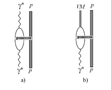
Figure 5: Electromagnetic diffractive processes in the dipole model with pomeron exchange. During the interaction time the photon polarizes into a quark-antiquak pair.  a:  $\gamma^{*}$ scattering; b:  electroproduction of vector mesons

In the dipole model the scattering amplitude is determined by a dipole cross section $\sigma_{\rm dip}(b_{\perp},u)$, which describes the interaction of a proton with a quark-antiquark pair with geometrical separation $b_{\perp}$ and longitudinal momentum fractions $u$ and $(1-u)$ respectively, and the overlap functions $\rho$ are given by the expressions (8),(9),(13), and (14).

The forward scattering amplitude is generically given by the expression

$${\cal T}_{0,\rm{pol}}=iW^{2}\,\int_{0}^{\infty}db_{\perp}\,$$ (27)

$$\int_{0}^{1}du\,{b_{\perp}}\,\sigma_{\rm{pol}}(b_{\perp},u,W)~{}\rho_{\rm{pol}}(Q^{2},u,b_{\perp})~{}.$$

For the energy dependence of the cross section we make the ansatz

$$\sigma_{\rm{pol}}(b_{\perp},u,W)=\sigma_{\rm dip}(b_{\perp},u)(W/W_{0})^{2\,\beta_{\rm{pol}}(b_{\perp},u)}~{}.$$ (28)

The energy-dependent scattering amplitude is, thus, given by

$${\cal T}_{0,\rm{pol}} = iW^{2}\,\int_{0}^{\infty}db_{\perp}\,\int_{0}^{1}du\,{b_{\perp}}\,\sigma_{\rm dip}(b_{\perp},u)\times$$

$$\qquad(W/W_{0})^{2\,\beta_{\rm{pol}}(b_{\perp},u)}\,\rho_{\rm{pol}}(Q^{2},u,b_{\perp})~{}.$$

Here again the index “$\rm{pol}$” refers to longitudinal and transverse polarizations. The total cross section is the sum of the longitudinally and transversely polarized forms.

Before we determine the power $\beta_{\rm{pol}}$ from experiment, we shortly discuss some general features of its energy behaviour. Since the effective power of the energy increases with increasing photon virtuality, the function $\beta_{\rm pol}(b_{\perp},u)$ in Eq. (28) must monotonously decrease with increasing $b_{\perp}$ and approach a value near 0.09 if the separation $b_{\perp}$ approaches the confinement scale (hadronic values). It is also very plausible that there exists a value $\beta_{\rm max}=\max[\beta_{\rm pol}(b_{\perp},u)]$. In the limit $W\to\infty$ the main contribution to the amplitude (III) comes from a region where $\beta(b_{\perp},u)$ reaches its maximum and therefore is driven to the behaviour ${\cal T}_{0}\sim(W/W_{0})^{\beta_{\rm max}}$. In this respect the model seems to correspond to a Regge cut with branch point at $\ell=\beta_{\rm max}$. However, the details of the high energy behaviour, depend crucially on the special form of the function $\beta_{\rm pol}(b_{\perp})$. In Appendix 2 we discuss the behaviour analytically.

From perturbation theory it is known that for small distances the dipole cross section behaves like $\sigma_{\rm dip}\sim b_{\perp}^{2}$, while for large distances it is model-dependent. We have studied two different cases, namely

$$\sigma_{\rm dip}(b_{\perp},u)=\left\{\begin{array}[]{ccc}C\,b_{\perp}^{2}&\mbox{ for }&b_{\perp}\leq b_{c}\\ C\,b_{c}^{2}&\mbox{ for }&b_{\perp}>b_{c}\end{array}\right.$$ (30)

and

$$\sigma_{\rm dip}(b_{\perp},u)=\left\{\begin{array}[]{ccc}C\,b_{\perp}^{2}&\mbox{ for }&b_{\perp}\leq b_{c}\\ 2C\,b_{c}(b-b_{c})&\mbox{ for }&b_{\perp}>b_{c}\end{array}\right.$$ (31)

with $b_{c}=5~{}\rm{GeV}^{-1}$, and found that the difference on the energy behaviour is very small. We have used in the following the cross section, Eq. (31). Comparison of the amplitude ${\cal T}_{0}$, Eq. (27), with the function $Y(Q^{2},b_{\perp})$, Eq. (11), shows that for $b<5$ GeV^-1 the amplitude ${\cal T}_{0}$ receives its main contribution from the region of $b_{\perp}$ where the function $Y(Q^{2},b_{\perp})$ is maximal. It is therefore suggestive to choose as function $\beta_{\rm po}(b,u)$ the right hand side of Eq. (18). But it turns out that in deep inelastic scattering the increase with energy of the the total $\gamma^{*}\,p$ hadronic cross section is much too slow for all values of $Q^{2}>1.5\mbox{ GeV}^{2}$. The reason for this behaviour is the slow decrease of the function $Y(Q^{2},b_{\perp})$, Eq. (11), with increasing $b_{\perp}$. If one chooses, however, the boost-invariant light-front separation $\zeta=\sqrt{u(1-u)}\;b_{\perp}$ as a scale, i.e. if one postulates

$$\sigma_{\rm pol}(b_{\perp},u,W)=\sigma_{\rm dip}(b_{\perp},u)(W/W_{0})^{2\,\beta_{\rm pol}(\zeta)},$$ (32)

one obtains with the functions

$$\tilde{\beta}_{T}(\zeta) = 0.0481\log\left[\frac{10.47}{\zeta^{2}}+6.541\right]$$ (33)

$$\tilde{\beta}_{L}(\zeta) = 0.0481\log\left[\frac{17.68}{\zeta^{2}}+6.530\right]$$

for the total $\gamma^{*}\,p$ cross section (structure functions) very satisfactory results. These expressions are derived from the maximum $\zeta(Q^{2})$ of the function

$$Z(Q^{2},\zeta) = \int_{0}^{1}du\,\sigma_{\rm dip}\left(\frac{\zeta}{u(1-u)},u\right)\times$$

$$\rho_{\gamma^{*}\gamma^{*},\rm pol}\left(Q^{2},u,\frac{\zeta}{u(1-u)}\right)~{},$$

and the relation between $Q^{2}$ and the power behaviour given by Eq. (7). Here the energy behaviour cannot be described by a single power and therefore one has to fit effective powers for a certain energy range. From the results obtained with Eqs. (III,32,33) the theoretically obtained curves in the range of energies 20 – 200 GeV (HERA range) we obtain the results displayed in Table 1, which compare favorably with the data Adloff:2001rw ; Zeus(11) . We give also the theoretical effective power fitted in the energy range 200 GeV - 2 TeV (accessible at LHC). As can be seen, the difference of values is only of about 10 %.

$Q^{2}$	$\lambda$(theory)		$\lambda$(experiment)
GeV2	HERA	LHC	HERA
2	0.183	0.205	0.159$\pm$0.016
5	0.213	0.237	0.196 $\pm$ 0.01
15	0.258	0.288	0.250 $\pm$0.01
25	0.280	0.310	0.274 $\pm$ 0.015
45	0.306	0.335	0.302 $\pm$ 0.02
60	0.319	0.348	0.332 $\pm$ 0.026
90	0.337	0.365	0.304 $\pm$ 0.05

Table 1: Values of the effective power $\lambda=\alpha_{\bf P}-1$ for the total $\gamma^{*}\,p$ cross section (structure function). Experimental values are from Adloff:2001rw ; Zeus(11) , the theoretical values are obtained with the energy-dependent dipole cross section (III) and the expressions (33). The HERA column indicates that the effective power is fitted in the HERA range of energies (ca 40 -200 GeV), whereas LHC is the theoretical value in a range accessible for LHC (200 GeV to 2 TeV).

The cross section obtained with Eqs. (III) and (33) can be well parameterized by an energy-dependent power,

$$\sigma_{\rm int}=C(W/W_{0})^{\delta(W)}$$ (35)

with

$$\delta(W)=E+\frac{F}{1000}\log[W/W_{0}]$$ (36)

The constants $E$ and $F$ are given in Table 6.

IV Description and prediction of diffractive vector meson production

In this section we compare data and predictions of the models discussed in Sects. II and III.

In Fig. 6 and Table 5 we display theoretical predictions for the powers $\delta$ and $\delta_{\rm int}$, that is, without and with shrinkage correction, as functions of the photon virtuality $Q^{2}$ for unpolarized elastic production of vector mesons in the ground state, together with the experimental results. The theoretical results for the $\omega$ meson production are not distinguishable from those of $\rho$ production. The long-dashed and the solid lines are obtained with the model discussed in Sect.II; the long-dashed curves represent the uncorrected power $\delta(Q^{2})$, obtained from Eq. (II.2), and the solid line represents $\delta_{\rm int}$, Eq. (II.2), that includes shrinkage corrections. The dotted line is the result of the model discussed in Sect. III, where an effective power $\delta$ has been extracted from the energy range $20\leq W\leq 200$ GeV. The shrinkage corrections to these results are the same as those for the results of Sect. II. The theoretical values of $\delta(Q^{2})$ calculated for $Q^{2}\geq 1$ GeV² and extrapolated to the value 0.36 at $Q^{2}=0$. The theoretical predictions of both models are well compatible with the data. The observed sharp increase of the power delta with $Q^{2}$ near $Q^{2}=0$ for the light vector mesons indicates that the rapidly varying shrinkage correction given by Eq. (24) is quite realistic. As can be seen, the shrinkage corrections are only important for $\rho$ production at $Q^{2}\leq 10\;\rm{GeV}^{2}$.

Figure 6: Predictions for the power $\delta$ and $\delta_{\rm int}$ as function of $Q^{2}$ for vector meson electroproduction and experimental values for this quantity: a) $\rho$-production Zeus(98) ; Zeus(99) ; Zeus(07) ; H1(00) ; H1(10) ; b) $\phi$-production Zeus(05) ; H1(10) ; c) $J/\psi$-production H1(06) ; H1(13) ; Zeus(02) ; Zeus(04) ; d) $\Upsilon$-production Zeus(09) ; LHCb(15) . The solid line and dashed lines represent respectively $\delta_{\rm int}$, Eq.(II.2), including the shrinkage correction, and $\delta$, Eq. (II.2), without shrinkage correction. The dotted lines are the results of the effective power as obtained from the model with an energy-dependent dipole cross section discussed in Sect. III, Eq. (III) with the energy dependence given by Eq. (33) without shrinkage correction.

In Fig. 7 data and the theoretically predicted energy dependence of $\rho$, $J/\psi$ and $\Upsilon$ production cross sections are displayed. In the model of Sect. II the energy dependence is represented by a single power $C\,W^{\delta}$ in the full energy range. Since emphasis in this paper is on energy dependence and the absolute values of the cross sections depend on details of the models, the constant $C$ is fitted to the data, and the values for the power $\delta$ are given by the model, both without shrinkage corrections, i.e. $\delta$ from Eq. (II.2) (dashed lines) and with shrinkage corrections, Eq. (II.2), solid line. The dotted lines are results of the dipole model of Sect. III, including shrinkage corrections according to Eq. (24).

The plot of $J/\psi$ photoproduction includes the most recent LHC data LHCb(14) ; Alice(14) . Here the influence of the shrinking correction is very small: $\delta(0)=0.69$ and $\delta_{\rm int}(0)=0.67$. The fit of the 58 points with free power gives the same value 0.67. Very recent values for $\Upsilon$ production together with theoretical predictions are also shown. Within errors they are compatible with both models.

In Table 6 we have collected the parameters of the theoretical curves displayed in Fig. 7, together with values of unconstrained fits to the data.

Figure 7: Energy dependence of photoproduction cross sections. In $\rho$ production Egloff ; EMC ; H1(96) ; Zeus-PL98 ; Zeus(07) , the results of Sect. II, with a scale-dependent Regge singularity, and those of Sect. III, with energy-dependent dipole cross section, are practically indistinguishable; the dashed line is the result without shrinkage correction, Eq.(19), and the solid includes the shrinkage correction, Eq.(25). In $J/\psi$ Fixed_Target ; Zeus(02) ; H1(13) ; LHCb(14) ; Alice(14) and $\Upsilon$ Zeus(98) ; H1_PLB2000 ; Zeus(09) ; LHCb(15) production, the shrinkage corrections are negligible. The solid lines are the result of Sect. II and the dotted line is the result of section III. For $J/\psi$ production a free fit coincides with the result of Sect. II. For $\Upsilon$ production it is shown with a dot-dashed line (the two old points in full circle and full square are excluded in this fitting). The precise parameters for the curves are given in Table 6.

The transverse and longitudinal wave functions are different and therefore we obtain different scales for the respective cross sections. This leads to a different energy behaviour for the two polarizations. According to the scale-dependent Regge pole, as discussed in Sect. II the ratio $R=\sigma_{L}/\sigma_{T}$ has the power behaviour

$$R=\frac{\sigma_{L}}{\sigma_{T}}=A\,W^{\delta_{\rm R}}~{},$$ (37)

with

$$\delta_{R}=\delta_{L}-\delta_{T}~{}.$$ (38)

The values of $\delta_{L}$ and $\delta_{T}$ are determined by Eq.(II.2) with the constants $A_{\rm VM,long},\,A_{\rm VM,trans},\,B_{\rm VM,long},\,B_{\rm VM,trans}$ of Table 4. In the model with an energy-dependent dipole cross section, see Sect. III, the corresponding expressions are obtained by calculating separately the longitudinal and transverse cross sections with the power functions (33).

In Fig. 8 a) - c) we show data Zeus(07) ; H1(10) ; E665(97) for the energy dependence of the polarization ratios $R=\sigma_{L}/\sigma_{T}$ for $\rho$ production at three values of $Q^{2}$. The solid lines are the theoretical predictions according to Sect.II, Eqs. (II.2,37,38). The multiplicative constant $A$ in Eq. (37) is fitted freely. The dotted lines are the results of the energy-dependent dipole model, Sect. III. We also show in dot-dashed lines the results of free fits to the data with unconstrained $A$ and $\delta_{R}$. At $Q^{2}=$ 7.5 and 22.5 GeV² the model gives good agreement for the energy dependence of $R$. In the last plot of the set, the data and the theoretical predictions for the power coefficients as functions of $Q^{2}$ are compared directly.

Figure 8: a)-c): Energy dependence of the ratio of longitudinal to transverse cross section of $\rho$ electroproduction for $Q^{2}=3.3,7.5$ and 22.5 GeV². The solid lines have the energy dependence predicted according to Eq.(37) with Eq.(II.2), the dotted lines the results of Sect. III, Eqs.(III),(18), and the dot-dashed lines are free best fits to the data. The data are from Zeus(07) ; H1(10) ; E665(97) ; d) Power $\delta_{R}$ for the energy dependence of the ratio as function of $Q^{2}$. The solid line is $\delta_{L}-\delta_{T}$ from Eq.(II.2), and the points with error bars are from the best fits to the data presented in the plots a)-c).

The experimental errors for the ratio $R$ are quite large and also the theoretical uncertainties in the small differences between $\delta_{L}$ and $\delta_{T}$ are large and both models are compatible with the data. The numerical values are given in Table 2.

$Q^{2}$	$\delta_{\rm tot}$			$\delta_{L}-\delta_{T}$
GeV2	Regge	Dipole		Regge	Dipole
		HERA	LHC		HERA
$\rho$
2	0.476	0.499	0.512	0.091	0.026
5	0.525	0.550	0.569	0.128	0.034
15	0.632	0.651	0.682	0.183	0.047
30	0.727	0.741	0.779	0.213	0.055
45	0.790	0.802	0.843	0.226	0.058
$J/\psi$
0	0.692	0.638	0.663	0.067	0.024
5	0.740	0.681	0.711	0.078	0.026
15	0.809	0.743	0.778	0.090	0.027
30	0.881	0.806	0.844	0.100	0.028
45	0.934	0.851	0.894	0.105	0.030
$\Upsilon$
0	1.046	0.955	0.995	0.060	0.013
15	1.073	0.977	1.020	0.062	0.013

Table 2: Theoretical values for the effective power $\delta$ of the energy dependence $W^{\delta}$ for integrated vector meson production cross section ($\delta_{\rm tot}$) and for the ratio of of longitudinal and transverse polarized cross section ($\delta_{L}-\delta_{T}$). The columns marked ”Regge” show the results of a scale dependent Regge pole as discussed in Sect. II, those under ”Dipole” are the results of the energy-dependent dipole cross section treated in Sect. III; the columns HERA indicate the effective power fitted in the HERA range of energies (ca 40 -200 GeV), while LHC gives the value in a range accessible to LHC (ca 200 GeV - 2 TeV).

V Summary and Conclusions

We have presented two simple phenomenological models which account for two striking features of electromagnetic diffractive processes, namely that the energy behaviour can be well described by a power behaviour and that the power parameter increases with increasing photon virtuality $Q^{2}$. It is remarkable that the power behaviour observed in elastic diffractive $J/\psi$ photoproduction in the HERA range of energies describes the data also up to 2 TeV. Such a behaviour is natural in Regge theory. In order to describe the observed dependence on the photon virtuality by a single pole we have to assume, however, that the position of this pole in the complex angular momentum plane depends on $Q^{2}$ for negative squared momentum transfer $t$ . In Sect. II we have shown that this behaviour is not in contradiction with general principles and gave the prescription for calculating the position of the scale-dependent Regge pole.

In Sect. IV it was shown that the model is very well compatible with experiment, and very recent data on $\Upsilon$ production at LHC LHCb(15) confirm it further. Also the concept of a scale-dependent slope of the Pomeron trajectory  Brower:2006ea is well compatible with the data H1(10) , as shown in Fig. 7.

A possible scenario for trajectories for $J/\psi$ and $\Upsilon$ photoproduction together with the conventional soft Pomeron trajectory is illustrated in Fig. 9. The intercept $\alpha_{P}(0)$ and the slope for $t<0$ are fixed by the model, see Eqs.(II.2), (24). For $t\gg 0$, where glueball states may be on the trajectory, the hadronic confinement scale becomes relevant and there it should coincide with the soft Pomeron, that is the Pomeron trajectory relevant for hadronic scattering.

A second model, based on a specific energy-dependence of the cross section of a quark-antiquark dipole, see Eq. (28), was discussed in Sect. III. If we choose as relevant scale for the energy dependence of the dipole cross section the boost-invariant light-front separation $\zeta=\sqrt{u(1-u)}\;b_{\perp}$ of the quark-antiquark pair,

$$\sigma_{\rm dip}(b_{\perp},u,W)=\sigma_{\rm dip}(b_{\perp},u)(W/W_{0})^{2\,\tilde{\beta}(\sqrt{u(1-u)}\;b_{\perp})}~{},$$ (39)

we also obtain with the expressions (33) good agreement with the data and specifically, that the effective power describing the energy-dependence varies only very little in the energy range up to 2 TeV. The energy-dependence obtained in this model corresponds to that of a Regge cut in the complex angular momentum plane. The main contribution to the discontinuity across the cut comes from the region $\ell=\tilde{\beta}(\zeta)$. This could be realized by a pole on the second sheet near the real axis, as indicated in Fig. 10. For positive values of $t$ this pole could emerge into the physical sheet and lead to particle poles for positive values of $t$ in the usual way.

Note added in proof:   Due to linear $t$-channel unitarity the partial wave amplitude for diffractive electroproduction of vector mesons, $\cal{T}_{\ell}$ in Eq.(3), will in general contain all contributions to the $p\bar{p}$ scattering amplitude, including the Pomeron at hadronic scales (soft Pomeron). The single power $\delta(Q^{2})$ used in Sec. II is therefore an effective power and can deviate from the corresponding value of the moving trajectory depicted in Fig. 9. We thank Peter Landshoff for pointing this out.

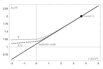
Figure 9: Scenario for scale-dependent Pomeron trajectories: the solid line is the trajectory relevant at hadronic scales (soft Pomeron), and the dashed and dotted lines represent the trajectories for $J/\psi$ and $\Upsilon$ photoproduction, respectively.

Figure 10: Scenario for a Regge cut in the angular momentum plane with a nearby pole on the second sheet. Such a situation could explain the energy-dependence obtained from the energy-dependent dipole cross section discussed in Sect. III.

VI Appendix

VI.1 Tables of Numerical Fits

	Transverse		Longitudinal
	$~{}\omega$	$N$	$~{}\omega$	$N$
	(GeV)		(GeV)
$\rho(770)$	$0.2809$	$2.0820$	$0.3500$	$1.8366$
$\omega(782)$	$0.2618$	$2.0470$	$0.3088$	$1.8605$
$\phi(1020)$	$0.3119$	$1.9201$	$0.3654$	$1.9191$
$J/\psi(1S)$	$0.6452$	$1.4752$	$0.7140$	$2.2769$
$\Upsilon(1S)$	$1.3333$	$1.1816$	$1.3851$	$2.7694$

Table 3: Parameters of the Brodsky-Lepage (BL) vector meson wave functions (II.2), taken from Dosch:2006kz ; Baltar:2009vp .

final state	$A_{\it fs,\rm pol}$			$B_{\it fs,\rm pol}$ [GeV2]
fs	trans	long	total	trans	long	total
$\gamma^{*}$	2.337	2.467	2.354	-0.003	-0.003	-0.005
$\rho$	10.594	5.658	7.565	3.971	2.248	2.699
$\phi$	9.117	5.578	6.658	3.711	2.454	2.449
$J/\psi$	6.968	5.329	5.644	20.021	15.975	14.696
$\Upsilon$	6.015	5.200	5.241	117.64	108.63	93.868

Table 4: Coefficients of the numerical fits of the average scale $\bar{b}_{\it fs}(Q^{2})$ , for the processes $\gamma^{*}{p}\to{\it fs}\,{p}$ with Eq. ((17)), for use in longitudinal, transverse and total (incoherent sum of the two cases) cross sections. $fs=\gamma^{*}$ refers to $\gamma^{*}\,{p}$ total cross section. The accuracy of the fit is better than 1% in the $Q^{2}$ range from 1 to 60 GeV² for photon scattering and $\rho,\,\phi$ production and from 0 to 60 GeV² for $J/\psi$ and $\Upsilon$ production. Remark: for $Q^{2}$ = 0 in $\rho$ and $\phi$ production, the relevant scale is the hadronic scale, chosen as $\bar{b}=5\mbox{ GeV}^{-1}$, with a soft Pomeron intercept 1.09.

Reaction	$\delta(Q^{2})$
$\gamma^{*}p\to\rho\,p,$ total	$0.1924\,\log(9.61827+1.1353\,Q^{2})$
trans	$0.1924\,\log(8.7997+0.5707\,Q^{2})$
long	$0.1924\,\log(11.5422+2.22949\,Q^{2})$
$\gamma^{*}p\to\phi\,p,$ total	$0.1924\,\log(10.1436+1.46565\,Q^{2})$
trans	$0.1924\,\log(9.3932+0.77065\,Q^{2})$
long	$0.1924\,\log(12.1579+2.29395\,Q^{2})$
$\gamma^{*}p\to J/\psi\,p,$ total	$0.1924\,\log(36.5274+2.03964\,Q^{2})$
trans	$0.1924\,\log(32.9435+1.31911\,Q^{2})$
long	$0.1924\,\log(46.6689+2.51262\,Q^{2})$
$\gamma^{*}p\to\Upsilon\,p,$ total	$0.1924\,\log(228.578+2.36527\,Q^{2})$
trans	$0.1924\,\log(214.809+1.77039\,Q^{2})$
long	$0.1924\,\log(293.23+2.63924\,Q^{2})$

Table 5: Functions $\delta(Q^{2})=4(\alpha_{\rm P}-1)$ given by Eq. (II.2).

Cross section parameters
$\sigma_{\rm int}(W)=C\,(W/W_{0})^{\delta},\;\delta=E+({F}/{1000})\log[W/W_{0}]$
Reaction	$Q^{2}$	$C$ [nb]	$\delta$		$\chi^{2}$
	[GeV2]		$E$	$F$
$\gamma\,p\to\rho\,p$	0
sect.II, wo. shrink.		2781$\pm$ 112	0.360	0	4.28
sect.II, w. shrink..		5283$\pm$ 209	0.190	0	0.635
sect.III, w. shrink.		5362$\pm$ 212	0.181	1.3	0.639
free fit of C and $\delta$		7351$\pm$ 1775	0.098	0	0.110
			$\pm$ 0.067
$\gamma^{*}\,p\to\rho\,p$	6
sect.II, wo. shrink.		11.93 $\pm$ 0.34	0.539	0	1.30
sect.II, w. shrink.		14.91 $\pm$ 0.37	0.486	0	0.666
sect.III, w. shrink.		13.26 $\pm$ 0.37	0.489	5.8	1.280
free fit of C and $\delta$		22.06 $\pm$ 9.82	0.393	0	0.227
			$\pm$ 0.106
$\gamma\,p\to J/\psi\,p$	0
sect.II, wo. shrink.		3.334 $\pm$ 0.045	0.692	0	0.845
sect.II, w. shrink.		3.624 $\pm$ 0.049	0.675	0	0.812
sect.III, w. shrink.		4.912 $\pm$ 0.067	0.579	6.2	1.044
free fit of C and $\delta$		3.61 $\pm$ 0.35	0.675	0	0.812
			$\pm$ 0.020
$\gamma\,p\to\Upsilon\,p$	0
sect.II, wo. shrink.		$(8.62\pm 1.65)10^{-4}$	1.04	0	0.667
sect.III, wo. shrink.		$(17.4\pm 3.5)10^{-4}$	0.862	10	0.463
free fit of C and $\delta$		$(44.6\pm 13.7)10^{-4}$	0.793	0	0.069
			$\pm$ 0.472

Table 6: Parameters of the curves displayed in Fig. 7. The integrated elastic diffractive cross sections are of the form $\sigma_{\rm int}(W)=C\,(W/W_{0})^{\delta},\;\delta=E+({F}/{1000})\log[W/W_{0}],\;W_{0}=1\,\rm{GeV}$. The constant $C$ is always fitted to the data, the fixed power $\delta$ in the row ”sect.II, wo. shrink.” is obtained from (19), in the row ”sect. II, w. shrink.” from (25); in the row ”sect.II, w. shrink.” the $W$-dependent power is a parametrization of the result obtained with the energy-dependent dipole cross section, as discussed in sect. 4, (28) ff, the shrinkage correction (24) is included. For $\Upsilon$ production the shrinkage correction is completely negligible. For comparison we show in the row ”free fit of C and $\delta$” the parameters of an unconstrained fit to the data.

VI.2 high-energyBehaviour of the Dipole Model

In this appendix we discuss the high-energybehaviour of the dipole model of Sect. III. For definiteness we investigate the simple case of elastic scattering of longitudinal virtual photons.

The scattering amplitude is, see Eqs. (9),(III),

$${\cal T}_{0}\sim iW^{2}\,\int_{0}^{\infty}db_{\perp}\,\int_{0}^{1}du\,{b_{\perp}}\,\sigma(b_{\perp},u)\times$$ (40)

$$\qquad(W/W_{0})^{2\,\beta(b_{\perp},u)}b_{\perp}~{}Q^{2}\,u^{2}(1-u)^{2}\,K^{2}_{0}(\epsilon b_{\perp})~{}.$$

Using as dipole cross section the simple quadratic form $\sigma(b_{\perp},u)=Cb_{\perp}^{2}$ we can write Eq. (40) as

$${\cal T}_{0}\sim iW^{2}\,\int_{0}^{\infty}d\zeta\,\zeta^{3}\,(W/W_{0})^{2\,\beta(\zeta)}\ ,Q^{2}\,K^{2}_{0}(Q\zeta)~{},$$ (41)

where we have made the phenomenologically successful assumption that the power function $\beta$ is a function of the light-front separation $\zeta=\sqrt{u(u-1)}\;b_{\perp}$, see Eq. (33). The behaviour of the integrand $I(\zeta)$ in Eq. (41) near $\zeta=0$ is $I(\zeta)\sim\zeta^{3}\log^{2}(Q\zeta)(W/W_{0})^{2\,\beta(\zeta)}$ and for large values $I(\zeta)\sim\zeta^{2}e^{-2Q\zeta}(W/W_{0})^{2\,\beta(\zeta)}$. We therefore investigate the integral

$${\cal T}_{a}=\int_{0}^{\infty}d\zeta\,\zeta^{3-\epsilon}\,(W/W_{0})^{2\,\beta(\zeta)}\,Q\,e^{-2Q\zeta}~{}.$$ (42)

We approximate ${\cal T}_{a}$ by the Gaussian integral

$${\cal T}_{a} = \exp[\phi(\zeta_{0})]\,\int_{0}^{\infty}d\zeta\,\exp[\frac{1}{2}(\phi^{\prime\prime}(\zeta_{0})(\zeta-\zeta_{0})^{2}]$$ (43)

$$\approx \sqrt{\frac{2\pi}{-\phi^{\prime\prime}(\zeta_{0})}}\;\exp[\phi(\zeta_{0})],$$

where

$$\phi(\zeta)=(3-\epsilon)\log\zeta-Q\zeta+\beta(\zeta)\,L;\quad L=\log\frac{W}{W_{0}}$$ (44)

and

$$\phi^{\prime}(\zeta_{0})=0~{}.$$ (45)

The power function $\beta(\zeta)$ has a negative derivative, therefore the value of $\zeta_{0}$ in the limit $W\to\infty$ is driven to $\zeta_{0}\to 0$. We assume that for $\zeta\to 0$ the function $\beta(\zeta)$ behaves as $\beta(\zeta)=\beta_{0}-\gamma\zeta^{n}$ . Then Eq. (45) is

$$0=\frac{3-\epsilon}{\zeta_{0}}-Q\zeta_{0}-n\gamma\zeta_{0}^{n-1}$$ (46)

and has in the large energy limit the real root

$$\zeta_{0}=\left(\frac{3-\epsilon}{2n\gamma L}\right)^{1/n}.$$ (47)

Inserting this into Eq. (43) yields for the high-energybehaviour of ${\cal T}_{a}$

$${\cal T}_{a}\sim\left(\frac{W}{W_{0}}\right)^{\beta_{0}}\,L^{-(4-\epsilon)/{n}}~{}.$$ (48)

The power behaviour of $cT_{a}$ is independent of $\epsilon$ and given by the maximal value of the power $\beta(\zeta)$, and therefore also the power of the amplitude ${\cal T}_{0}$ is given by $\beta_{0}$. The logarithmic corrections however depend on the specific behaviour of the function $\beta(\zeta)$.

References

- (1) V. N. Gribov and L. N. Lipatov, Yad. Fiz. 15,781 (1972) [Sov. J. Nucl. Phys. 15, 438 (1972)]
- (2) G. Altarelli and G. Parisi, Nucl. Phys. B 126, 298 (1977)
- (3) Y. L. Dokshitzer, Zh. Eksp. Teor. Fiz. 73, 1216 (1977) [Sov. Phys. JETP 46, 641 (1977)]
- (4) A classical textbook is P.D.B. Collins, An Introduction to Regge Theory ( Cambridge University Press, Cambridge, England,1977)
- (5) G.N. Watson, Proc. Royal Soc. A95 , 83 (1918) .
- (6) A. Sommerfeld, Partial Differential Equation in Physics (Academic Press, New York, 1949)
- (7) A. Donnachie and P. V. Landshoff, Phys. Lett. B 296, 227 (1992)
- (8) V. S. Fadin, E. A. Kuraev and L. N. Lipatov, Phys. Lett. B 60, 50 (1975)
- (9) E. A. Kuraev, L. N. Lipatov and V. S. Fadin, Zh. Eksp. Teor. Fiz. 72, 377 (1977) [Sov. Phys. JETP 45, 199 (1977)]
- (10) I. I. Balitsky and L. N. Lipatov, Yad. Fiz. 28, 1597 (1978) [Sov. J. Nucl. Phys. 28 822 (1978)]
- (11) M. Ciafaloni and G. Camici, Phys. Lett. B 430, 349 (1998) [hep-ph/9803389].
- (12) V. S. Fadin and L. N. Lipatov, Phys. Lett. B 429, 127 (1998) [hep-ph/9802290].
- (13) A. Donnachie and P. V. Landshoff, Phys. Lett. B 437, 408 (1998)
- (14) H. G. Dosch, E. Ferreira and A. Kramer, Phys. Rev. D 50, 1992 (1994) [hep-ph/9405237].
- (15) H. G. Dosch, T. Gousset and H. J. Pirner, Phys. Rev. D 57, 1666 (1998) [hep-ph/9707264].
- (16) G. Kulzinger, H. G. Dosch and H. J. Pirner, Eur. Phys. J. C 7, 73 (1999) [hep-ph/9806352]
- (17) A. Donnachie, H. G. Dosch and M. Rueter, Eur. Phys. J. C 13, 141 (2000)
- (18) A. Donnachie and H. G. Dosch, Phys. Lett. B 502, 74 (2001)
- (19) A. Donnachie and H. G. Dosch, Phys. Rev. D 65, 014019 (2001)
- (20) H. G. Dosch and E. Ferreira, Eur. Phys. J. C 29, 45 (2003)
- (21) H. G. Dosch and E. Ferreira, Eur. Phys. J. C 51, 83 (2007)
- (22) V. L. Baltar, H. G. Dosch and E. Ferreira, Int. J. Mod. Phys. A 26, 2125 (2011)
- (23) R. Aaij et al. (LHCb Collaboration), J. Phys. G 41 , 055002 (2014)
- (24) B. Abelev et al.(Alice Collaboration), Phys. Rev. Lett. 113, 232504 (2014)
- (25) R. Aaij et al. (LHCb Collaboration), arXiv: 1505.08139 [hep-ex]
- (26) R. C. Brower, J. Polchinski, M. J. Strassler and C. I. Tan, J. High Energy Phys. 12 (2007) 005
- (27) Y. Hatta, E. Iancu and A. H. Mueller, J. High Energy Phys. 01 (2008) 026 [arXiv:0710.2148 [hep-th]].
- (28) C. Adloff et al. (H1 Collaboration), Phys. Lett. B 520 , 183 (2001)
- (29) V. Radescu (H1 and ZEUS Collaborations), arXiv:1308.0374 [hep-ex]
- (30) G.P. Lepage and S.J. Brodsky, Phys. Rev. D 22, 2157 (1980)
- (31) K. A. Olive et al. (Particle Data Group Collaboration), Chin. Phys. C 38 090001 (2014)
- (32) F. D. Aaron et al., J. High Energy Phys. 05 (2010) 032
- (33) S. Chekanov et al. (Zeus Collaboration), Phys. Lett. B 697, 184 (2011)
- (34) J. Breitweg et al., Eur. Phys. J. C 2, 247 (1998)
- (35) M. Derrick et al., Eur. Phys. J. C 6, 603 (1999)
- (36) S. Chekanov et al., PMC Physics A 6 (2007)
- (37) C. Adloff et al., Eur. Phys. J. C 13, 371 (2000)
- (38) S. Chekanov et al., Nucl.Phys B 718 , 3 (2005)
- (39) A. Aktas et al., , Eur. Phys. J. C 46, 585 (2006)
- (40) C. Alexa et al. (H1 Collaboration), Eur. Phys. J. C 73, 2466 (2013)
- (41) S. Chekanov et al., Eur. Phys. J. C 24, 345 (2002)
- (42) S. Chekanov et al., Nucl. Phys. B 695, 3 (2004)
- (43) S. Chekanov et al., Phys. Lett. B 680, 4 (2009)
- (44) N. Nikolaev and B. G. Zakharov, Z. Phys. C 53, 331 (1992)
- (45) C. Ewerz and O. Nachtmann, Ann. Phys. (Amsterdam) 322 1635, 1670 (2007) [hep-ph/0604087]
- (46) C. Ewerz, A. von Manteuffel and O. Nachtmann, Phys. Rev. D 77 074022 (2008) [arXiv:0708.3455 [hep-ph]]
- (47) R.M. Egloff, P.J.Davis, G.J.Luste, J.F.Martin and J.D.Prentice , Phys. Rev. Lett. 43 , 657 (1979)
- (48) J.J. Aubert et al. [EMC Collaboration] , Phys. Lett B 161, 203 (1985) ; J. Ashman et al. [EMC Coll.] , Zeit.Phys. C 39, 169 (1988)
- (49) S. Aid et al. , (H1 Collaboration), Nucl.Phys. B463 3 (1996)
- (50) J. Breitweg et al. (Zeus Collaboration), Phys. Lett. B 437, 432 (1998)
- (51) B.H. Denby et al., Phys. Rev. Lett. 52 , 795 (1984) ; M.E. Binkley et al., Phys. Rev. Lett. 48, 73 (1982)
- (52) C. Adloff et al. (H1 Collaboration), Phys. Lett. B 483 (2000) 23
- (53) M. R. Adams et al., Zeit. Phys. C 74 , 237 (1997)