Nearby stars as gravitational wave detectors

Abstract

Sun-like stellar oscillations are excited by turbulent convection and have been discovered in some 500 main sequence and sub-giant stars and in more than 12,000 red giant stars. When such stars are near gravitational wave sources, low-order quadrupole acoustic modes are also excited above the experimental threshold of detectability, and they can be observed, in principle, in the acoustic spectra of these stars. Such stars form a set of natural detectors to search for gravitational waves over a large spectral frequency range, from $10^{-7}$ Hz to $10^{-2}$ Hz. In particular, these stars can probe the $10^{-6}$ Hz – $10^{-4}$ Hz spectral window which cannot be probed by current conventional gravitational wave detectors, such as SKA and eLISA. The PLATO stellar seismic mission will achieve photospheric velocity amplitude accuracy of $~{}{\rm cm/s}$. For a gravitational wave search, we will need to achieve accuracies of the order of $10^{-2}{\rm cm/s}$, i.e., at least one generation beyond PLATO. However, we have found that multi-body stellar systems have the ideal setup for this type of gravitational wave search. This is the case for triple stellar systems formed by a compact binary and an oscillating star. Continuous monitoring of the oscillation spectra of these stars to a distance of up to a kpc could lead to the discovery of gravitational waves originating in our galaxy or even elsewhere in the universe. Moreover, unlike experimental detectors, this observational network of stars will allow us to study the progression of gravitational waves throughout space.

1. Introduction

Astronomers had not expected that stars, other than the Sun, could provide us with the observed wealth of high quality seismic data, surpassing in diversity and quantity the data gathered from the Sun itself. Previously, the GOLF experiment aboard the Solar and Heliospheric Observatory mission Gabriel et al. (1995) measured the global acoustic oscillations of the Sun from a spatially unresolved entire solar disk of Doppler velocity data (Turck-Chieze et al. 2004). Presently, following an identical strategy, the COROT and Kepler space missions (Baglin et al. 2006; Gilliland et al. 2010), by measuring the light integrated from the entire visible star’s surface, have searched for global oscillations in more than 150,000 main sequence, subgiant and red giant stars (Borucki et al. 2009; Verner et al. 2011). A sample of more than five hundred low mass subgiants and main sequence stars were discovered to have rich Sun-like acoustic oscillation spectra filled with tens of velocity amplitude peaks (Chaplin et al. 2014). Similar oscillations have been found in more than 12,500 K-G giant stars. Although their acoustic spectra are very distinct from those of main sequence stars, as a consequence of their quite distinct structure (Hekker et al. 2011), these oscillations still qualify as Sun-like oscillations. As in the Sun, these oscillations are excited by turbulent convection and intrinsically damped by the radiation and the turbulence of the outer layers of the star. Such seismic observational surveys are able to follow in a systematic and continuous manner the pulsation spectra of the Sun and stars in the solar neighbourhood within a range of up to one thousand parsecs distance. These surveys observed fields of stars in the galactic plane, as well as in a few directions above and below it (Miglio et al. 2012), as in the Kepler mission which has been observing stars 13^o above the galactic plane in the Cygnus region. This local gravitational system of celestial bodies made of many stars of different sizes and masses, constituted of single stars, binaries or multi-stellar systems, as well as a few stellar clusters (Corsaro et al. 2012), is a natural network of detectors for gravitational radiation. In this work we argue that this natural network of stars will allow us to search for gravitational wave imprints in the oscillation spectra of single stars, or for contemporaneous signatures of the same gravitational wave event on the spectra of two or more close stars. It will also allow us to follow the progression of a gravitational wave through space, across the spectra of several stars - when it passes through a stellar cluster - and to monitor its progression as it approaches the Earth.

The most likely source of gravitational waves able to stimulate quadrupole modes in Sun-like stars are short-period binaries of two compact objects such as white dwarfs, or even neutron stars and massive black holes. Low mass binaries are the leading gravitational source candidates, despite having relatively weak gravitational wave emission, as they are numerous and are located in close proximity to the Solar System (Amaro-Seoane P. et al. 2013). More than 50 ultra-compact binaries, with a size of about a fraction of the solar radius and a period shorter than one hour, have been discovered at a distance between 50 and 700 parsec, an example being the cataclysmic variable star AM CVn located at a distance of 606 parsecs from Earth (Roelofs et al. 2007). AM CVn is a binary system where a white dwarf accretes matter from a companion star, leading to the formation of an accretion disc with continuous strong emission in UV and X-rays, and with occasional outbursts. If seismic surveys are set to observe and monitor stars near these binaries, this could lead to the discovery of gravitational waves.

The idea that gravitational radiation could excite the normal modes of vibration of celestial bodies such as the Earth and the Sun was originally discussed by Dyson (Dyson 1969) and many other papers have followed up this idea. Most recently McKernan et al. (2014) have estimated the gravitational radiation that is absorbed by stars and Siegel & Roth (2011) are among others to suggest the impact of gravitational waves on solar oscillations. Gravitational wave detection through stars and resonant mass detectors (Aguiar et al. 2006; Gottardi 2007) both work based in a similar principle. In the latter case, the detection is done by accurately measuring the tiny variation of the detector size when one or more modes are excited by a passing gravitational wave (Sathyaprakash & Schutz 2009). In stars detection is feasible by monitoring the variations of velocity of the modes at the surface. Some aspects of the analysis for stars are similar to the case of spherical resonant mass detectors.

2. The acoustic spectra of the Sun and stars

Stars, like musical instruments, vibrate in a multitude of eigenmodes. The discrete sequence of frequencies for stellar oscillations can be labelled by two independent integers: the degree of the mode $l,$ which is the degree of the spherical harmonic related with the horizontal eigenfunction; and the order of the mode $n$ which measures the number of nodes of the radial eigenfunction along the radius. For each value $l,$ there is a sequence of resonant acoustic modes that are labelled with $n.$ The latter ones correspond to the fundamental tone and overtones of a musical instrument. Whole-disk observations of stars through the seismic space missions detect only the large luminosity variations in the stellar surface; therefore, these observations are only sensitive to the lowest values of $l$ ($l\leq 3$). The angular frequency of such low-degree acoustic modes satisfies

$$\omega_{N}=(n+1/2\;l+\alpha_{o})\bar{\omega}+\zeta_{N}$$ (1)

where $N$ is a subscript that defines a specific eigenmode $N\equiv(n,l)$, $\alpha_{o}$ and $\bar{\omega}$ are constants and $\zeta_{N}$ is a second order term that can be neglected when $n$ is large (Lopes 2001). The constant $\bar{\omega}$ is relates do $\nu_{o}$ by $\nu_{o}=\bar{\omega}/2\pi$. This last quantity is known as the large separation. The frequencies with the same degree are separated apart by $\nu_{o}$. This quantity is equal to $1/\left(2\int_{0}^{R}dr/v_{s}(r)\right)$, the time taken for the sound wave to travel with a speed $v_{s}(r)$ from the surface to the center of the star and return. According to equation (1) for $\omega_{N}$, $\nu_{o}$ is equal to $(\omega_{(n,l)}-\omega_{(n-1,l)})/2\pi$. The previous equation with minor adjustments has been shown to be valid for many main sequence and red giant stars (Mosser et al. 2011; Corsaro et al. 2012). Table 1 lists the frequencies of the quadrupole mode as measured by the GOLF experiment. When no observational data is available, we show in italics the predicted values for the standard solar model (Lopes & Turck-Chieze 2013). One can notice that for frequencies of the acoustic modes of low degree, the disagreement between theory and observation is at most of the order of a few percent (see Turck-Chieze & Lopes 2012, and references therein). Table 1 lists the frequencies for the quadrupole modes.

Recent observations have shown that many main-sequence, subgiant and red giant stars have a spectrum of acoustic oscillations identical to the Sun, with only minor differences (Mosser et al. 2011; Chaplin et al. 2014). The properties of a star’s spectrum are characterized by three main quantities: the large separation, the frequency at which the amplitude of the spectrum of oscillations is maximum, and the effective temperature of the star. At present, when these quantities are available, they provide the most reliable method for determining the mass and radius of a star (Chaplin & Miglio 2013). It has been shown from observational data, that homology ratios for mass, radius and effective temperature hold between the Sun and these stars. In particular, the large separation scales as:

$$\left(\frac{\bar{\omega}}{\bar{\omega}_{\odot}}\right)=\left(\frac{M}{M_{\odot}}\right)^{1/2}\left(\frac{R}{R_{\odot}}\right)^{-3/2},$$ (2)

where $M$ and $R$ are the mass and radius of the star. Equally, $\bar{\omega}_{\odot}/2\pi$, $M_{\odot}$ and $R_{\odot}$ are the solar equivalent quantities. In the case of the Sun, the mean large separation $\bar{\omega}/2\pi$ is of the order of $135\;\mu$ Hz (as computed from table 1).

Table 1Quadrupole acoustic modes
Observational data and Standard solar model

n	Freq.	$\eta_{n}$	$\chi_{n}$	$L_{n}$	$M_{N}$	$\Sigma_{n}$	$Q_{n}$	$V_{n}$	$T_{n}^{\star}$	$V_{n,u}$
	($\mu Hz$)	($\mu Hz$)	(no-dim)	$({\rm cm})$	$(M_{\odot})$	(${\rm cm^{-2}\;Hz}$)	(no-dim)	$({\rm cm\;s^{-1}})$	(no-dim)	$({\rm cm\;s^{-1}})$
			$\times 10^{-4}$	$\times 10^{7}$	$\times 10^{-3}$		$\times 10^{+8}$	$\times h_{-20}$	$\times 10^{-3}$	$\times h_{-20}$
$f$	$\mathit{347.10}$	$\mathit{2.9\;10^{-7}}$	$-6.7432$	$2.347$	$0.5854$	$94.931$	$38$	$1.4\,10^{-6}$	$2.7$	$7.1\;10^{-8}$
$p_{1}$	$\mathit{382.26}$	$\mathit{2.9\;10^{-6}}$	$-11.038$	$3.841$	$1.1148$	$98.315$	$4.1$	$2.6\,10^{-7}$	$23$	$4.0\;10^{-8}$
$p_{2}$	$\mathit{514.48}$	$\mathit{1.6\;10^{-5}}$	$+2.1193$	$0.737$	$0.1594$	$0.9671$	$1.0$	$1.7\,10^{-8}$	$72$	$4.6\;10^{-9}$
$p_{3}$	$\mathit{664.06}$	$\mathit{7.4\;10^{-5}}$	$-0.6286$	$0.219$	$0.0466$	$0.0424$	$0.28$	$1.8\,10^{-9}$	$210$	$8.2\;10^{-10}$
$p_{4}$	$\mathit{811.33}$	$\mathit{2.6\;10^{-4}}$	$+0.2133$	$0.074$	$0.0154$	$0.0025$	$0.10$	$2.6\,10^{-10}$	$506$	$1.9\;10^{-10}$
			$\times 10^{-6}$	$\times 10^{5}$	$\times 10^{-6}$		$\times 10^{6}$		$\times 10^{0}$
$p_{5}$	$\mathit{959.23}$	$\mathit{7.9\;10^{-4}}$	$-8.2377$	$2.867$	$1.0733$	$2\;10^{-4}$	$3.8$	$4.7\,10^{-11}$	$1.1$	($5.0\;10^{-11}$)
$p_{6}$	$\mathit{1104.28}$	$\mathit{2.1\;10^{-3}}$	$+3.4804$	$1.211$	$0.4537$	$2\;10^{-5}$	$1.7$	$9.8\,10^{-12}$	$2.3$	($1.5\;10^{-11}$)
$p_{7}$	$\mathit{1249.78}$	$\mathit{5.3\;10^{-3}}$	$-1.5051$	$0.524$	$0.1968$	$2\;10^{-6}$	$0.74$	$2.1\,10^{-12}$	$4.7$	($4.6\;10^{-12}$)
$p_{8}$	$1394.68\pm 0.01$	$0.01$	$+0.6836$	$0.238$	$0.0880$	$2\;10^{-7}$	$0.33$	$4.9\,10^{-13}$	$9.4$	($1.5\;10^{-12}$)
$p_{9}$	$1535.865\pm 0.006$	$0.04$	$-0.3109$	$0.108$	$0.0392$	$3\;10^{-8}$	$0.12$	$8.9\,10^{-14}$	$24$	($4.4\;10^{-13}$)
			$\times 10^{-8}$	$\times 10^{4}$	$\times 10^{-9}$		$\times 10^{4}$		$\times 10^{1}$
$p_{10}$	$1674.534\pm 0.013$	$0.08$	$+14.946$	$1.082$	$18.647$	$3\;10^{-9}$	$6.7$	$2.6\,10^{-14}$	$4.1$	$----$
$p_{11}$	$1810.349\pm 0.015$	$0.10$	$-7.8242$	$0.520$	$10.06$	$6\;10^{-10}$	$4.1$	$9.0\,10^{-15}$	$6.2$	$----$
$p_{12}$	$1945.800\pm 0.02$	$0.14$	$+4.3862$	$0.272$	$6.106$	$2\;10^{-10}$	$2.9$	$3.8\,10^{-15}$	$8.3$	$----$
$p_{13}$	$2082.150\pm 0.02$	$0.21$	$-2.5981$	$0.153$	$4.0176$	$3\;10^{-11}$	$2.1$	$1.7\,10^{-15}$	$10.9$	$----$
$p_{14}$	$2217.69\pm 0.03$	$0.31$	$+1.5564$	$0.054$	$2.7101$	$9\;10^{-12}$	$1.9$	$1.0\,10^{-15}$	$11.4$	$----$
$p_{15}$	$2352.29\pm 0.03$	$0.40$	$-0.9562$	$0.033$	$1.9063$	$3\;10^{-12}$	$1.8$	$6.4\,10^{-16}$	$11.1$	$----$
$p_{16}$	$2485.86\pm 0.03$	$0.44$	$+0.6204$	$0.022$	$1.4536$	$1\;10^{-12}$	$1.7$	$4.2\,10^{-16}$	$11.1$	$----$
$p_{17}$	$2619.64\pm 0.04$	$0.53$	$-0.4180$	$0.014$	$1.1950$	$4\;10^{-13}$	$1.5$	$2.6\,10^{-16}$	$12.2$	$----$
$p_{18}$	$2754.39\pm 0.04$	$0.57$	$+0.2908$	$0.010$	$1.0383$	$2\;10^{-13}$	$1.5$	$1.8\,10^{-16}$	$12.0$	$----$

3. Interaction between gravitational waves and acoustic modes

Within the framework of general relativity, far from the source of gravitational radiation, the space-time metric tensor is distorted relative to flat spacetime (Minkowski) value by a very small spatial component, $h_{\rm ij}$. In a Galilean coordinate frame whose origin coincides with the center of the star, the stellar material experiences a force proportional to $h_{\rm ij}$. Thus, the quadrupole modes of vibration of the star will be excited by gravitational waves when the frequency of the incoming waves is close to the eigenfrequency of the modes. In this case, the time variation of the amplitude of the mode of vibration is described by a harmonic damped oscillator with an excitation source proportional to $h_{\rm ij}$. As usual, we express the tensor $h_{\rm ij}$ as the sum of spherical components $h_{m}$, for which the $m$ (azimuthal order) is an integer such that $|m|\leq l$. The dynamics of general relativity implies that only non-radial modes of degree larger that two can be excited. Of these, the forcing of the quadrupole modes is normally the greatest. Actually, the differential rotation in the Sun and Sun-like stars can also split the $\omega_{N}$ (equation 1) leading to a subset of $2m+1$ frequencies for each $l,$ which in the case of quadrupole modes corresponds to five values differing between them only by a few microHz. Nevertheless, as we are only concerned about the amplitude of the modes, in this study the solution will be found for a generic value of $m.$ As we restrict our attention to quadrupole acoustic modes of order $n$ with fixed (undistinguished) $m$ for which $|m|\leq 2$, in the remainder of this article the fiducial mode will be represented as $N$ or simply by $n$, meaning $N\equiv(n,2,"m")$.

The strength by which the quadrupole modes of the star are stimulated by gravitational radiation depends on the absorption cross-section for gravitational radiation or its integrated value (in frequency), the quality factor, and the amplitude of the root mean square velocity at the surface of the star, also known as the photospheric velocity. The theoretical calculation of these quantities is computed in an identical manner to gravitational wave detectors. Accordingly, the impact of a plus polarized monochromatic gravitational wave, such as $h_{\star}\cos{(\omega t)}$, with a strain $h_{\star}$ and frequency $\omega$, averaged over several cycles is estimated as follows:

- First, the absorption cross-section for gravitational waves by the star, $\sigma_{\rm abs}(\omega)$, is defined by expressing the balance between the amount of energy $E_{\rm abs}$ which is absorbed by the star and the amount of incident energy $E_{\rm in}$ on the star’s surface:

$$\frac{dE_{\rm abs}}{dt}=\sigma_{\rm abs}(\omega)\frac{dE_{\rm in}}{dAdt}.$$ (3)

where $dE_{\rm in}/dAdt$ is the energy arriving per unit of time, per unit area.

- Second, the average $dE_{\rm in}/dAdt$ value for the case of a monochromatic gravitational wave is equal to $c^{3}h_{\star}\omega^{2}/(32\pi G)$ where c and G are the values of the velocity of light in vacuum and Newton’s gravitation constant. Moreover, the gravitational wave averaged over several cycles leads to $\langle\cos{(\omega t)}\rangle$, which is equal to 1/2.

- Third, the energy $E_{\rm abs}$ that is absorbed by the star per unit of time by each resonant mode $N$ averaged for a few cycles, is equal to the product of the gravitational wave force $F_{\rm gw}(t)$ and the velocity of the mode $\dot{\xi}_{N}$ where $\xi_{N}$ is the amplitude of the stimulated quadrupole mode. The gravitational force $F_{\rm gw}(t)$ is equal to $M_{N}L_{n}\ddot{h}_{m}$, where $M_{N}$ and $L_{n}$ are the modal mass and the modal length of the mode, both of which depend on the properties of the acoustic eigenfunction, and $\ddot{h}_{m}$ is the second derivative of $m$’s spherical component, the perturbation tensor $h_{ij}$. The modal length of the mode $L_{n}$ is an effective length of the mode equivalent to the size of a resonant detector. $L_{n}$ is unique for each acoustic mode, $L_{n}=1/2\;R\;|\chi_{n}|$ where $\chi_{n}$ is a coefficient that depends of the eigenfunction $\xi_{N}$:

$$\chi_{n}=\frac{3}{4\pi\bar{\rho}_{\star}}\int_{0}^{1}\rho(r)\left[\xi_{r,n}(r)+3\xi_{h,n}(r)\right]r^{3}dr.$$ (4)

where $\rho$ and $\bar{\rho}_{\star}$ are the density profile and mean density of the star, and $\xi_{r,n}$ and $\xi_{h,n}$ are the radial and horizontal components of the quadrupole modal eigenfunction $\xi_{N}$, respectively. As originally computed for a resonant detector (e.g., Maggiore 2008), the absorbed energy per unit time is expressed as

$$\frac{dE_{abs}}{dt}\equiv\langle F_{\rm gw}(t)\dot{\xi}_{N}\rangle=\frac{M_{N}h_{\star}^{2}\;L_{n}^{2}\;\eta_{n}\omega^{6}}{(\omega^{2}-\omega_{n}^{2})^{2}+4\eta_{n}^{2}\omega^{2}},$$ (5)

where $\eta_{n}$ is the damping rate of the mode.

Equations (3) and (5) relate to the energy of the incident gravitational wave with the energy absorbed by the acoustic mode $N$, from which is obtained the average absorption cross-section:

$$\sigma_{\rm abs}(\omega)=\frac{M_{N}\eta_{n}L_{n}^{2}\;\omega^{4}}{(\omega^{2}-\omega_{n}^{2})^{2}+4\eta_{n}^{2}\omega^{2}}\;\frac{32\pi G}{c^{3}}$$ (6)

The response of a mode to a gravitational perturbation is better evaluated by the integral of the absorption cross-section, $\Sigma_{n}=\int\sigma_{\rm abs}(\omega)d\omega/2\pi$ for which the limits of the integral correspond to the frequency interval of the gravitational wave-packet. However, as the function $\sigma_{\rm abs}(\omega)$ only is significantly different from zero near each resonance frequency $\omega_{n}$, conveniently, without much loss of accuracy, the limits of the integral can be replaced by $-\infty$ and $+\infty$. For the same reason, the second term in the right-side of the equation (6) is expanded in $(\eta_{n}/\omega_{n})$.

$\Sigma_{n}$ near the resonance frequency, reduces to

$$\Sigma_{n}=\pi\chi_{n}^{2}\;\frac{M_{N}G}{c}\;\left(\frac{R\omega_{n}}{c}\right)^{2},$$ (7)

thus, $M_{N}=E_{N}M$ where $E_{N}$ is the normalized inertia of the mode. This approximate result shows that the integrated cross-section is independent of the quality factor of the mode, $Q_{n}\equiv\omega_{n}/(2\eta_{n})$. This occurs because at the peak $\sigma(\omega)$ is proportional to $Q_{n}$, so that $Q_{n}$ cancels in $\int d\omega\sigma(\omega)$. Using equation (1), $\Sigma_{n}=F_{n}\;({M_{N}G}/{c})({R\bar{\omega}}/{c})^{2}$ where $F_{n}=\pi\chi_{n}^{2}\;(n+1+\alpha_{o})^{2}$. In the particular case that the sound speed is constant, for instance equal to the average sound speed $\bar{v}_{s}$, $\bar{\omega}=\pi\bar{v}_{s}/R$. $\Sigma_{n}$ becomes identical to the one computed for a resonant mass detector, $\Sigma_{n}=F_{n}^{\star}\;({M_{N}G}/{c})\;({v}_{s}/{c})^{2}$ where $F_{n}^{\star}=\pi^{3}\chi_{n}^{2}\;(n+1+\alpha_{o})^{2}$ (Maggiore 2008).

The relevant observable that will allow us to identify the impact of gravitational waves in an oscillation mode is the phostopheric velocity that is computed as $V_{n}^{2}(\omega_{n})\equiv 1/({2\eta_{n}M_{N}})\;dE_{abs}/dt$ (Goldreich & Keeley 1977). Therefore, using equation (5), we obtain

$$V_{n}(\omega_{n})=\frac{h_{\star}L_{n}\omega_{n}^{2}}{\alpha_{s}\eta_{n}}.$$ (8)

In the previous equation, we introduce the numerical constant $\alpha_{s}$ which is equal to $2\sqrt{2}$, for which the exact value is fixed by observations. Since the amplitude of the strain decreases with the inverse of the distance, $h_{\star}$ is computed as $h_{\star}=d_{\earth}/d_{\star}\,h_{\earth}$, where $d_{\earth}$ and $d_{\star}$ are the distances of the source of gravitational radiation to the Earth and to the Sun-like star, and $h_{\earth}$ is the current strain prediction for the Earth detectors. An illustrative example is shown in Figure 1.

The photospheric velocity, as shown in equation (8), relates to the excitation of quadrupole modes of frequency $\omega_{n}$ by a monochromatic gravitational wave with the same frequency $\omega$, i.e., $\omega=\omega_{n}$. Nevertheless, in some cases as noticed by McKernan et al. (2014), $\omega$ drifts across the frequency $\omega_{n}$ like it occurs during the inspiral phase of binary systems. The magnitude of the frequency drift $\dot{\omega}$ is mostly dependent of the chip mass of the binary $M_{c}$, as $\dot{\omega}\approx 3\left(GM_{c}/c^{3}\right)^{5/3}\omega^{11/3}$ (Maggiore 2008). The contribution of $\dot{\omega}$ for the excitation of a quadrupole mode is only relevant if the duration of the gravitational time $\tau_{f}=1/\sqrt{\dot{\omega}}$ is smaller than the damping time of the mode $\tau_{n}=1/(2\eta_{n})$, or if the ratio $T^{\star}_{n}\equiv\tau_{f}/\tau_{n}$ is smaller than one.

The steady-state (or saturated) limit corresponds to $T^{\star}_{n}\gg 1$ (or $\tau_{f}\gg\tau_{n}$) for which $\dot{\omega}$ can be neglected in the calculation of the photospheric velocity (equation 8). However, as shown by McKernan et al. (2014) in the reverse case of undamped oscillations, for which $T^{\star}_{n}\ll 1$ (or $\tau_{f}\ll\tau_{n}$), the slow frequency variation of the gravitational wave must be taken into account, accordingly $\omega_{n}$ must be replaced by $\omega_{n}+\dot{\omega}_{n}\tau$, where $\tau$ is the time difference to the resonance. The calculation of $\tau_{f}$ is given by $4.81\times 10^{9}\left(M_{c}/M_{\odot}\right)^{-5/6}\left(\omega_{n}/{\rm mHz}\right)^{-11/6}$ (Maggiore 2008).

Rathore et al. (2005) have estimated that the averaged energy transfer to quadrupole mode by a slow varying frequency gravitational source is given by $\pi h_{\star}^{2}/(4\dot{\omega}_{n})$. Accordingly, the energy absorbed by a stellar quadrupole mode per unit time in the undamped limit ($T^{\star}_{n}\ll 1$, subscript $u$) is expressed as $\left({dE_{abs}}/{dt}\right)_{u}=T^{\star}_{n}\;\left({dE_{abs}}/{dt}\right)$ where $\left({dE_{abs}}/{dt}\right)$ corresponds to the solution given by equation (5). $\left({dE_{abs}}/{dt}\right)_{u}$ relates with the work done by an external slow varying gravitational source (see McKernan et al. (2014) for details). Accordingly, the photospheric velocity in the undamped limit is reduced in relation to the steady-state limit (i.e., $V_{n}$), it reads $V_{n,u}(\omega_{n})={T^{\star}_{n}}^{1/2}\;V_{n}(\omega_{n})$. Equally, $\sigma_{\rm abs,u}(\omega)$ and $\Sigma_{n,u}$ are also reduced in the case of the undamped limit, as these quantities are obtained by multiplying $\sigma_{\rm abs}(\omega)$ (equation 6) and $\Sigma_{n}$ (equation 7) by the same $T^{\star}_{n}$ factor.

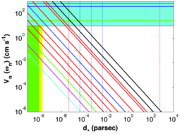
Figure 1.— Impact of a gravitational wave in a Sun-like star detector: The photospheric velocity $V_{n}(\omega_{n})$ (in $cm\;s^{-1}$) for quadrupole acoustic modes is a function of the distance to the gravitational wave source, as predicted by equation (8). In the case of modes with $n\leq 5$ (see Table 1), the photospheric velocity is computed in the undamped limit, i.e., the photospheric velocity corresponds to $V_{n,u}={T^{\star}_{n}}^{1/2}\;V_{n}$. As an example of a gravitational wave source, we choose the compact binary system AM CVn (e.g., Solheim et al. 1998; Roelofs et al. 2007) located at a distance $d_{\earth}=606$ pc, which has a size smaller than $0.5$ of the solar radius and a orbital period of $\sim 1029s$, for which the strain amplitude for Earth detectors is predicted to be $h_{\earth}=2\;10^{-22}$. Accordingly, the strain amplitude $h_{\star}$ of the arriving gravitational wave to the Sun-like star is computed as $h_{\star}=3\;10^{-14}/d_{\star}(AU)$. The vertical dashed-lines correspond to the distance of the gravitational wave source to the star’s detector: Sun (magenta) and a Sun-like star located at a distance of 1 AU (red) or 10, 100 and 1000 AU (blue). The vertical green and yellow areas correspond to $0.5$ and $1.0$ of the solar radius. The oblique lines correspond to the quadrupole modes: $p_{i}$ with $i=0,1,2,4,5,6$ (red), $p_{i}$ with $i=3,7,12,18$ (blue, green, magenta, cyan) correspond to $h_{\star}=3\;10^{-12}/d_{\star}(AU)$ with $h_{\earth}=10^{-20}$ (see Table 1). For reference, we show $p_{0}$ and $p_{1}$ (black lines) corresponding to the steady-state (or saturated) limit. The horizontal cyan band ($V_{n}\geq 1.0\;cm\;s^{-1}$) defines the expected $V_{n}$ threshold of the Plato mission. To illustrate the variety of sun-like star oscillations, we show several maximum $V_{n}$ measurements (horizontal lines): Sun (green), Procyon (blue) and $\nu$ Ind (magenta) stars (see main text). See Table 1 for further information about quadrupole modes.

The integrated absorption-cross section (equation 7) and the photospheric velocity (equation 8) for a star can be scaled to the Sun. Using the eigenfrequency equation (1) retaining only the first term, and the scale relation (2), the integrated absorption-cross section reads

$$\frac{\Sigma_{n}}{\Sigma_{n\odot}}=\left(\frac{\chi_{n}}{\chi_{n\odot}}\right)^{2}\left(\frac{E_{n}}{E_{n\odot}}\right)\left(\frac{M}{M_{\odot}}\right)^{2}\left(\frac{R}{R_{\odot}}\right)^{-1}$$ (9)

and the photospheric velocity reads

$$\frac{V_{n}}{V_{n\odot}}=\left(\frac{\chi_{n}}{\chi_{n\odot}}\right)\left(\frac{\eta_{n}}{\eta_{n\odot}}\right)^{-1}\left(\frac{M}{M_{\odot}}\right)\left(\frac{R}{R_{\odot}}\right)^{-2}$$ (10)

where the subscript $\odot$ denotes the Sun. The equivalent expressions for the undamped/unsaturated case ($T^{\star}_{n}\ll 1$) are obtained by multiplying the right-side of both previous equations by the ratio $(T^{\star}_{n}/T^{\odot}_{n})$ and $(T^{\star}_{n}/T^{\odot}_{n})^{1/2}$, respectively.

4. The sensitivity of star’s detectors to gravitational waves

Similarly to convectional resonant mass detectors, the stimulation of quadrupole oscillations in stars by an external gravitational radiation source depends on the integrated cross-section and the quality factor. Table 1 lists these quantities, as well as the amplitude of the photospheric velocity for the quadrupole acoustic modes in the Sun. Moreover, we also computed the photospheric velocity in the case of undamped oscillations and the ratio $T^{\star}_{n}$. In this study we chose as fiducial gravitational wave source the AM CVn binary system ($M_{c}=0.248\;M_{\odot}$), for which $\tau_{f}$ is equal to $\sim 1.54\times 10^{10}\;\left(\omega_{n}/{\rm mHz}\right)^{-11/6}{\rm sec}$. Existing observations and other theoretical quantities computed from an updated standard solar model (e.g., Lopes & Turck-Chieze 2013) are also summarized in the table. The quadrupole modes that have the largest integrated cross-sections and quality factors, as well as the largest photospheric velocity, are the modes of lower order. In the following, we give the reasons why Sun-like stars are good gravitational wave detectors:

- It follows from equation (7) that the integrated cross-section of a mode depends on the modal mass and the length of the mode, as well as the sound speed in the interior of the star. Because stars have much larger masses than convectional resonant mass detectors, their integrated cross-section is many orders of magnitude larger. In the Sun, low order modes have a $\Sigma_{n}$ that is 17 or 20 orders of magnitude (if we consider the steady-state or undamped limits respectively) larger than the current detectors, such as Mario Schenberg (Aguiar et al. 2006), Minigrial (Gottardi 2007) and Allegro (Mauceli et al. 1996). Gottardi (2007) estimates a $\Sigma_{n}$ of the order of $9.8\,10^{-22}{\rm cm^{-2}\,Hz}$ for a high performance resonant mass detector. Even for high order modes ($n\sim 15$) the Sun, as a detector, performs better by a ten-magnitude factor. More massive stars have a fractionally smaller $\Sigma_{n}$ than the Sun. Hence, from equation (9), it follows that $\Sigma_{n}$ increases with $M^{2}$ and decreases with $R$, as for most of the observed Sun-like stars, like red giants (Mosser et al. 2012), the smaller mass corresponds to $0.5\,M_{\odot}$ and the largest radius to $15\,R_{\odot}$, which leads to a maximum reduction of $\Sigma_{n}$ by a negligible factor of $0.02$. The variation of $\chi_{n}$ and $E_{n}$ among these stars also introduces important corrections to $\Sigma_{n}$, in many cases, this should increase the value of $\Sigma_{n}$. Therefore the net result found for the Sun also holds for many of these stars.

- Stars respond to gravitational radiation as a truly high Q oscillator. As shown in table 1, this is particularly relevant in the case of low order modes. Actually, the $Q_{n}$ for small $n$ is 1 to 2 orders of magnitude better than for current detectors. Gottardi (2007) estimates that $Q_{n}\sim 10^{7}$ for a CuAl alloy spherical detector. In Sun-like stars, such high Q is due to the predicted low rates, believed to be caused by the damping processes related with radiation and turbulence convection of the upper layers of the star. This behaviour is most relevant for main sequence and subgiant stars (with $M$ varying from $0.95\;M_{\odot}$ to $2.0\;M_{\odot}$) for which current theoretical models predict that the $\eta_{n}$ for low $n$ modes is of the order of $10^{-5}$ to $10^{-7}$ (Houdek et al. 1999; Baudin et al. 2005). It was also found that for global acoustic modes ($l\leq 3$) , that $\eta_{n}$ is independent of $l$ and always increases with $n.$ Besides, $\eta_{n}$ always decreases with the mass of the star and also as its age increases. This behaviour is similar for red giant stars. Recent seismic data has shown that the average damping rate $\langle\eta_{n}\rangle$ of Sun-like stars increases with the effective temperature. This relation holds not only for main sequence and subgiant field stars, but equally for red giant stars, some of which were discovered in open stellar clusters (e.g., Corsaro et al. 2012). As the $\langle\eta_{n}\rangle$ of red giant stars is two orders of magnitude smaller than for the Sun’s case, we expect that the $\eta_{n}$ of low order modes varies by a similar amount, leading to an increase of $Q_{n}$. Nonetheless, a smaller quality factor could be beneficial, as a lower $Q$ factor increases the possibility of quadrupole modes being easily excited by gravitational radiation.

- According to equation (8), the low order quadrupole modes are the ones for which the photospheric velocity is predicted to have the largest value. The velocities of the modes of higher order are not so high. The increase of the photospheric velocity depends of the quantities on the ratio $\omega_{n}^{2}/\eta_{n}$ which for low $n$ have not yet been measured for the Sun, and only theoretical predictions are available, as shown in italics in table 1. Nevertheless, both quantities are predicted by theoretical models, which successfully reproduce the observational data at higher frequencies. The $L_{n}$ and its related quantity $\chi_{n}$ are the other critical quantities that affect the photospheric velocity. Unlike for a typical detector, $L_{n}$ and $\chi_{n}$ decrease rapidly with $n$. As shown in equation (4), this is due to the fact that the density in the star decreases with the increase of the radius, and the depth reached by the acoustic eigenfunction $\xi_{N}$ decreases as n increases. As shown in table 1, $L_{n}$ is only significant for modes of low order. The decrease of $L_{n}$ and $\eta_{n}^{-1}$ with $n$ is the main reason for the rapid decrease of photospheric velocity with $n$. Nonetheless, we notice that in the case of the frequency of the gravitational wave drifts during the excitation of the quadrupole mode, the maximum $V_{n}$ attained will be reduced by up to several orders of magnitude, as we discuss in the previous section. Table 1 shows the photospheric velocity computed for a strain of $10^{-20}$, which for the first low order modes, is predicted to have a maximum amplitude of $10^{-6}\;{\rm cms^{-1}}$ or $7\;10^{-8}\;{\rm cms^{-1}}$ respectively for the steady-state ($T^{\star}_{n}\gg 1$) and undamped ($T^{\star}_{n}\ll 1$) limit cases. In this study, the reduction of $V_{n,u}$ over steady-state is as much as two orders of magnitude, and will be greatest for modes with the largest cross-sections. Indeed, the excitation of quadrupole modes by gravitational waves is limited at low order by the fact that oscillations are unsaturated, and at higher order modes because these have small cross sections to the impact of gravitational waves (see Table 1).

Thus in order for gravitational waves in the star acoustic spectrum to be detected, it would be necessary for $V_{n}$ to be larger than the current signal-yo-noise ratio instrumental threshold. A current estimation of this threshold for a future interplanetary space mission (Appourchaux et al. 2009), made from an average of the 50 modes observed by the GOLF experiment (Turck-Chieze et al. 2004; García et al. 2007; Jimenez & Garcia 2009) during a period of 10 years fixes the observation limit of 1 $\sigma$ level between $10^{-2}{\rm cm\;s^{-1}}$ and $3\,10^{-4}{\rm cm\;s^{-1}}$. Nevertheless, for the next planed seismic missions, TESS (Ricker et al. 2014) and Plato (Rauer 2013) the minimum $V_{n}$ measured is expected to be of the order of $1\;{\rm cm\;s^{-1}}$. Although, this precision is not sufficient to detect gravitational waves with current sun-like stars, it is possible that goal to be achieved in a next generation of seismic instruments, as we show in figure 1 if a precision of $10^{-2}\;{\rm cm\;s^{-1}}$ is attained, this type of detection could be successful in some specific multi-body stellar systems. In the remaining of the article, this value is used as a detectability threshold for a future space mission. Indeed, it follows that the $V_{n}$ for the $f$-mode, $p_{1}$-mode and $p_{2}$-mode increases above the threshold of $10^{-2}\;{\rm cm\;s^{-1}}$, if $d_{\star}$ is smaller than 10 AU, as illustrated schematically in Figure 1 for the case of a fiducial compact binary as the AM CVn binary. Obviously, if the strain is 2 orders of magnitude larger, it will be much easier to successfully detect the gravitational radiation (cf. Figure 1).

The variation of mass and radius of the star affects the amplitude of the photospheric velocity, and it follows from equation (10) that $V_{n}$ increases with $M$ and decreases with $R^{2}$. Thus ignoring the variation of $\chi_{n}$ and $\eta_{n}$, and taking the minimum $M$ and maximum $R$ values from the recent list of observed Sun-like stars (e.g., Mosser et al. 2012; Chaplin et al. 2014), at $0.5\,M_{\odot}$ and $15\,R_{\odot}$, the photospheric velocity is reduced by a factor $2\,10^{-3}$. One such example is the star KIC 5822889 for which $V_{n}$ is $0.01V_{n\odot}$ For other stars the effect is the reverse, as for KIC 7970740 for which $V_{n}\approx 1.3V_{n\odot}$ (Chaplin et al. 2014). This is a rough estimate, because these calculations do not account for the potential differences coming from $T^{\star}_{n}$, $\eta_{n}$ and $\chi_{n}$. In particular, notice the case of quadrupole modes with very low $n$ for which the excitation by gravitational waves occurs in the unsaturated case, $T^{\star}_{n}\equiv\tau_{f}/\tau_{n}$ reduces further the value of $V_{n}$. In the case of the AM CVn compact binary, $T^{\star}\sim 10^{-3}$ assuming that $\eta_{n}$ is similar to the Sun, $V_{n}$ reduces by a further $\sqrt{10^{-3}}$ factor. For instance, $\eta_{n}$ for low $n$ is of the order of $10^{-6}\mu Hz$ and does not change much among this type of star, as $\chi_{n}$ increases for more massive stars, due to the increase of the density in the star’s core. Although Sun-like stars can have different $\chi_{n}$ and $\eta_{n}$, the low $n$ modes should be always the ones with the largest velocity amplitudes.

Actually, in many spectra of Sun-like stars, acoustic modes were found with large photospheric velocities, believed to be stimulated by the turbulent convection in the envelopes of these stars. Figure 1 shows the maximum photospheric velocities measured for a few of the most well-known stars  other than the Sun - with $20$ cm$s^{-1}$ (Jimenez & Garcia 2009), Procyon with $38$ cm$s^{-1}$ (Kervella et al. 2004; Leccia et al. 2007; Arentoft et al. 2008; Bedding et al. 2010) and the sub-giant star $\nu$ Ind with $650$ cm $s^{-1}$ (Bedding et al. 1996, 2006; Carrier et al. 2007; Kjeldsen et al. 2008). This behavior follows the well-known scaling equation for the maximum velocity amplitude of acoustic modes $V_{\rm n,max}$ excited by turbulent convection, which increases with the luminosity and decreases with mass and effective temperature of the star (Kjeldsen & Bedding 2011). This equation remains valid for red giant stars, as found in observations for which $V_{\rm n,max}$ varies from 10 to 800 cm s^-1 (Samadi et al. 2013).

Figure 2.— Comparison of Sun-like star’s detectors with current gravitational waves detectors: (i) The range of frequencies for probing for gravitational wave sources is evaluated from the observed acoustic spectra of Sun-like stars: main sequence and subgiant stars show oscillations from 2 10^-4 Hz to 10^-2 Hz (Arentoft et al. 2008); and red giant stars from $10^{-7}$ Hz to $5\;10^{-3}$ Hz (Mosser et al. 2013) (magenta shadowed area). (ii) The range of strain amplitudes possible to probe by natural star detectors, depends mainly from the amplitude generated by the gravitational wave source, as unlike for gravitational wave detectors on Earth, Sun-like stars can be located quite close to the source. As for the example shown in Figure 1 if a natural star detector is located at a distance of 1 AU from the gravitational wave source (red vertical line in Figure 1), for which $h_{\star}(1AU)\sim 3\,10^{-14}$, this corresponds to $h_{\earth}\sim 2\,10^{-22}$ on Earth, leading to an effective strain gain of $10^{+8}$. Equally, if the star detector is located at 1 solar radius from the gravitational wave source $h_{\star}(1R_{\odot})\sim 5\,10^{-12}$. At these distances all the low order modes ($n\leq 4$) of the star are stimulated by the gravitational waves generated by the compact stellar binary. The strain sensitivity curve of the different gravitational detectors and most common sources of gravitational waves were adapted from Moore (2014).

The acoustic mode frequencies of Sun-like stars can probe gravitational waves in the range from 10^-7 Hz to 10^-2 Hz, which overlaps with the gravitational radiation frequency range that will be probed by eLISA (Amaro-Seoane P. et al. 2013) for the high frequency range and EPTA (Ferdman et al. 2010) and SKA (Johnston et al. 2007) in the low frequency range. More significant even is the possibility of probing the range from 10^-6 Hz to 10^-5 Hz, a frequency range for which no experiment has yet been planned. This is illustrated in Figure 2. In the low frequency range, this region corresponds to the predictions of stochastic background radiation and supermassive binaries. In the high frequency range, it corresponds to unresolvable galactic binaries, extreme mass ratio inspirals and resolved galactic binaries (Sathyaprakash & Schutz 2009). One of the targets of eLISA will be nearby ultracompact binaries, such as the binary system AM CVn discussed in this article as a template. The strategy of using Sun-like stars as detectors will enable us to determine the impact of gravitational waves in the photospheric velocities of quadrupole modes, or, at least, to fix an upper limit on the strain of the gravitational waves generated by these sources. The $h$ sensitivity of eLISA will be $10^{-16}$ to $10^{-20}$ for the frequency range of $10^{-5}$ Hz to $10^{-2}$ Hz which is not sufficient to detect the gravitational waves produced by the AM CVn binary system, predicted to have a strain amplitude on Earth of $10^{-22}$ (cf. Figure 2). Yet, a future seismic mission could detect such gravitational waves in stars like the Sun located at a distance of either 10 AU or 1000 AU from this binary system, if the $h_{\earth}$ is of the order of $10^{-22}$ or $10^{-20}$, respectively. As shown in figure 1 the quadrupole modes of lowest orders will be stimulated by these gravitational waves producing photospheric velocities possibly above the observational limit of the detector. Moreover, other stars like sub-giant and red giant stars could scan other parts of the frequency range of the gravitational wave spectrum, including outside of the current range of detectors. Red giant stars with oscillations within the frequency range from $10^{-7}$ Hz to $10^{-3}$ Hz (Mosser et al. 2013) can be used to explore events related with super-massive binaries for which the strain on Earth is predicted to be of the order of $10^{-14}$ (see Moore 2014, and references therein).

5. Stellar systems and the detectability of gravitational waves

Central to the applicability of using sun-like stars as detectors is to find an oscillating star for which the photospheric velocity is above the threshold of detectability (cf. Figure 1). As discussed previously for the sun’s case, the photospheric velocity is of the order $10^{-8}\;{\rm cm\;s^{-1}}$ for a strain of $h_{-20}=1$ (see Table 1). Therefore for such a signal to be detected it is necessary to find a way to increase the photospheric velocity by 4 orders of magnitude. Two obvious possibilities are to choose stars for which their $\chi_{n}$ sensitive to gravitational waves is larger than the sun (like red-giants), or stronger gravitational wave sources (like the coalescence of black holes with a typical strain $\sim 10^{-17}$). Here, nevertheless the discussion is focused in another point: the possibility of the next generation of stellar missions discovering gravitationally bound multi-body systems with a compact binary and an oscillating sun-like star, for which the seismic instrument has the necessary accuracy to measure the impact of gravitational waves in the acoustic oscillations.

The probability of finding an oscillating star nearly enough to a compact binary is quite small, nevertheless, recently many gravitationally bound multi-body systems of three or more stars have been discovered, which gives some hope that one of such unique systems could actually be found. The current theory of stellar formation, predicts the existence of many binary, triple and higher multiplicity stellar systems. This has also been confirmed by many astronomical observations. Tokovinin (2014) studied the multiplicity of multi-body systems within 67 pc of the Sun and found that 13% of stellar systems have three or more components. Raghavan et al. (2010) estimated that as much as 8% are three-body systems, and Rappaport et al. (2013) using Kepler data estimated that 20% of close binaries have tertiary companions. Moreover, Holberg et al. (2002) have reported that within the first 20pc of the Sun, 25% of white dwarf are in binary systems.

Several triple systems have been discovered with characteristics relatively close to the ideal case discussed in this article, compact binaries (Meliani et al. 2000) with a star companion. In particular, the COROT and Kepler missions have discovered several specific triple star systems (Southworth 2014), like the KOI-126, a very small hierarchical triple system composed by a short-period binary of two 0.2$M_{\odot}$ stars orbiting by an evolved G-star (with a mass of 1.3$M_{\odot}$ and radius of 2.0 $R_{\odot}$) (Carter et al. 2011). The semi-major axis of the inner and outer binaries are 0.021 AU and 0.24 AU respectively. Another equally different example is the triple system J0337+1715, a compact system with a total dimension smaller than 2 AU, where a close binary of a white dwarf and neutron star is orbited by a second white dwarf (Ransom et al. 2014). Equally, Kilic et al. (2014) have discovered a close binary of white dwarfs WD 0931+444 that possibly have an M dwarf companion, although for the moment sun-like oscillations have not yet been discovered in M dwarfs (Rodríguez-López et al. 2015).

Finally there is the possibility, that among the many binary systems formed by a white dwarf and sun-like star discovered by the Kepler mission (Rappaport et al. 2015; Southworth 2014), like KOI-3278 (Kruse & Agol 2014), the white dwarf could actually be a close compact binary. Equally, higher order multiplicity system could also be worth investigating to look for compact binaries and oscillating stars (Riddle et al. 2015), like some 2+2 quadruple systems which have an outer separation of 500 AU.

Although asteroseismology is not as precise as helioseismology, if the optimal triple or higher order multi-body stellar system is found the accuracy of the future (and possibly present) stellar seismic missions could be sufficient to detect gravitational waves. Currently, the Plato mission observations for quiet stars, expects that for an exposure time of only 15 minutes to be sufficient to average out the perturbing signal well below $1\;{\rm m\;s^{-1}}$, and in some cases the noise even gets down $10\;{\rm cm\;s^{-1}}$ in about 20-30 minutes (Rauer 2013). It is possible that in cases of much longer time exposures, the compute photospheric velocities will be well below $1\;{\rm cm\;s^{-1}}$ (Rauer et al. 2014).

Altogether, by using this proposed method, main-sequence, sub-giant and red giant stars increase significantly the detection power and the spectral range for identifying gravitational wave imprints in acoustic oscillations.

6. Summary and Conclusion

Stars like the Sun have the potential to become ideal detectors of gravitational waves. Not only do they have a high scattering cross-section for gravitational waves, high quality factors and very likely large photospheric velocities, but they also may be located near strong gravitational wave candidates. Helio and asteroseismology allow us to probe these natural detectors with very high precision. Indeed, for each oscillating star, the radial modes and dipole modes can be used to determine the oscillator characteristics like the damping rates, which is critical to allow us to disentangle the stimulation caused by gravitational radiation from the excitation produced by turbulent convection. The standard theory of stellar pulsations by turbulent convection establishes that low order acoustic modes ($l\leq 3$) are equally excited and their excitation depends uniquely on the frequency of the mode and not on the degree. This model has already been proven to be consistent with observations for a large range of frequencies. Therefore, the radial and dipole modes with frequencies near the frequencies of the quadruple modes of low order can be used as reference to isolate the stimulation of low order quadrupole modes by gravitational waves from the stellar self-excitation.

Although main-sequence, subgiant and red giant stars, all have the possibility to be good detectors of gravitational waves, subgiants and red giants have a substantial advantage in relation to main-sequence stars, as their rich spectrum has shown the existence of quadrupole mixed modes (Benomar et al. 2013). These modes behave like gravity waves in the star’s core and like acoustic waves in the stellar surface. Accordingly, their eigenfunctions have large amplitude in both the core and the surface. As a consequence the modal length, $L_{n}$ is much larger for these stars than in the Sun’s case, so that their photospheric velocities are larger than the ones predicted for the Sun.

The Sun and similar stars also have quadrupole gravity modes that can be excited by gravitational waves. These modes have very large modal lengths $L_{n}$ compared with acoustic modes, because eigenfunctions of gravity modes have larger amplitudes in the star’s core. Unfortunately, gravity modes are strongly attenuated when they propagate through the convection region and as such it is very difficult to observe them in the star’s surface. Actually, in the Sun it has been a matter of dispute whether a few gravity modes candidates were observed successfully (Turck-Chieze et al. 2004).

The group of all oscillating stars in the solar neighborhood within one thousand parsecs radius, constitutes the largest detector ever for gravitational radiation. Stars have some advantages over the current Earth detectors. There are thousands of oscillating stars scattered throughout space, some of which can be found relatively near gravitational wave sources. Alignments of stars between the source and the Solar System can monitor the progression of gravitational waves throughout space, which can be use as a test to probe General Relativity, a goal that is difficult to achieve with present man-made detectors.

Equally important is the fact that such a new method to prove gravitational wave radiation could probe an important part of the spectral gravitational radiation window – from one micro Hz to 100 micro Hz (cf. Figure 2), which is not probed by current detectors and it is not expected to be probed by any planned future ones. Actually, this is part of the reason why there are not many theoretical predictions for gravitational radiation emitted in this spectral frequency range. Among the possible candidates to produce the gravitational waves in this frequency range, there is the merger of intermediate mass black holes in the final year prior to the coalescence (for example a merger of a hundred solar mass black hole with an one million solar mass black hole) that could originate from the high mass tail of the initial mass function of Population III stars (Madau & Rees 2001). The strain of these events varies from $10^{-23}$ to $10^{-17}$ depending on the chirp mass of the binary system in the coalescence phase (Bender & Pollack 2004).

References

- Aguiar et al. (2006) Aguiar, O. D., Andrade, L. A., Barroso, J. J., et al. 2006, Classical and Quantum Gravity, 23, 239
- Amaro-Seoane P. et al. (2013) Amaro-Seoane, P., et al. 2013, GW Notes, 6, 4–110
- Appourchaux et al. (2009) Appourchaux, T., Burston, R., Chen, Y., et al. 2009, Experimental Astronomy, 23, 491
- Arentoft et al. (2008) Arentoft, T., Kjeldsen, H., Bedding, T. R., et al. 2008, The Astrophysical Journal, 687, 1180
- Baglin et al. (2006) Baglin, A., et al. 2006, in ”Proceedings of The CoRoT Mission Pre-Launch Status - Stellar Seismology and Planet Finding (ESA SP-1306). Editors: M. Fridlund, A. Baglin, J. Lochard and L. Conroy ISBN 92-9092-465-9., p.33 http://adsabs.harvard.edu/abs/2006ESASP1306…33
- Baudin et al. (2005) Baudin, F., Samadi, R., Goupil, M. J., et al. 2005, Astronomy and Astrophysics, 433, 349
- Bedding et al. (1996) Bedding, T. R., Kjeldsen, H., Reetz, J., & Barbuy, B. 1996, Monthly Notices of the Royal Astronomical Society, 280, 1155
- Bedding et al. (2006) Bedding, T. R., Butler, R. P., Carrier, F., et al. 2006, The Astrophysical Journal, 647, 558
- Bedding et al. (2010) Bedding, T. R., Kjeldsen, H., Campante, T. L., et al. 2010, ApJ, 713, 935 ApJ, 713, 935
- Belkacem et al. (2013) Belkacem, K., Samadi, R., Mosser, B., Goupil, M. J., & Ludwig, H. G. 2013, in Progress in Physics of the Sun and Stars: A New Era in Helio- and Asteroseismology. Proceedings of a Fujihara Seminar held 25-29 November, 61
- Bender & Pollack (2004) Bender, P. L., & Pollack, S. E. 2004, Coevolution of Black Holes and Galaxies, 4
- Benomar et al. (2013) Benomar, O., Bedding, T. R., Mosser, B., et al. 2013, The Astrophysical Journal, 767, 158
- Bertello et al. (2000) Bertello, L., Varadi, F., Ulrich, R. K., et al. 2000, The Astrophysical Journal, 537, L143
- Borucki et al. (2009) Borucki, W., Koch, D., Batalha, N., et al. 2009, Transiting Planets, 253, 289
- Carrier et al. (2007) Carrier, F., Kjeldsen, H., Bedding, T. R., et al. 2007, A&A, 470, 1059
- Carter et al. (2011) Carter, J. A., Fabrycky, D. C., Ragozzine, D., et al. 2011, Science, 331, 562
- Chaplin et al. (1997) Chaplin, W. J., Elsworth, Y., Isaak, G. R., et al. 1997, Monthly Notices of the Royal Astronomical Society, 288, 623
- Chaplin & Miglio (2013) Chaplin, W. J., & Miglio, A. 2013, Annual Review of Astronomy and Astrophysics, 51, 353
- Chaplin et al. (2014) Chaplin, W. J., Basu, S., Huber, D., et al. 2014, The Astrophysical Journal Supplement, 210, 1
- Corsaro et al. (2012) Corsaro, E., Stello, D., Huber, D., et al. 2012, The Astrophysical Journal, 757, 190
- Dyson (1969) Dyson, F. J. 1969, Astrophysical Journal, 156, 529
- Ferdman et al. (2010) Ferdman, R. D., van Haasteren, R., Bassa, C. G., et al. 2010, Classical and Quantum Gravity, 27, 4014
- Gabriel et al. (1995) Gabriel, A. H., Grec, G., Charra, J., et al. 1995, Solar Physics, 162, 61
- García et al. (2007) García, R. A., Turck-Chièze, S., Jiménez-Reyes, S. J., et al. 2007, Science, 316, 1591
- Garcia et al. (2001) Garcia, R. A., Regulo, C., Turck-Chieze, S., et al. 2001, Solar Physics, 200, 361
- Gilliland et al. (2010) Gilliland, R. L., Jenkins, J. M., Borucki, W. J., et al. 2010, The Astrophysical Journal Letters, 713, L160
- Goldreich & Keeley (1977) Goldreich, P., & Keeley, D. A. 1977, Astrophysical Journal, 211, 934
- Gottardi (2007) Gottardi, L. 2007, Physical Review D, 75, 22002
- Grigahcène et al. (2005) Grigahcène, A., Dupret, M. A., Gabriel, M., Garrido, R., & Scuflaire, R. 2005, Astronomy and Astrophysics, 434, 1055
- Hekker et al. (2011) Hekker, S., Gilliland, R. L., Elsworth, Y., et al. 2011, Monthly Notices of the Royal Astronomical Society, 414, 2594
- Holberg et al. (2002) Holberg, J. B., Oswalt, T. D., & Sion, E. M. 2002,ApJ, 571, 512
- Houdek et al. (1999) Houdek, G., Balmforth, N. J., Christensen-Dalsgaard, J., & Gough, D. O. 1999, Astronomy and Astrophysics, 351, 582
- Jimenez & Garcia (2009) Jimenez, A., & Garcia, R. A. 2009, The Astrophysical Journal Supplement, 184, 288
- Johnston et al. (2007) Johnston, S., Bailes, M., Bartel, N., et al. 2007, Publications of the Astronomical Society of Australia, 24, 174
- Kervella et al. (2004) Kervella, P., Thévenin, F., Morel, P., et al. 2004, Astronomy and Astrophysics, 413, 251
- Kilic et al. (2014) Kilic, M., Brown, W. R., Gianninas, A., et al. 2014, MNRAS, 444, L1 MNRAS, 444, L1
- Kjeldsen & Bedding (2011) Kjeldsen, H., & Bedding, T. R. 2011, Astronomy and Astrophysics, 529, L8
- Kjeldsen et al. (2008) Kjeldsen, H., Bedding, T. R., Arentoft, T., et al. 2008, The Astrophysical Journal, 682, 1370
- Kruse & Agol (2014) Kruse, E., & Agol, E. 2014, Science, 344, 275 Science, 344, 275
- Leccia et al. (2007) Leccia, S., Kjeldsen, H., Bonanno, A., et al. 2007, Astronomy and Astrophysics, 464, 1059
- Lopes (2001) Lopes, I. P. 2001, MNRAS, 321, 615
- Lopes & Turck-Chieze (2013) Lopes, I., & Turck-Chieze, S. 2013, The Astrophysical Journal, 765, 14
- Madau & Rees (2001) Madau, P., & Rees, M. J. 2001, ApJ, 551, L27
- Maggiore (2008) Maggiore, M. 2008, Gravitational Waves, Volume 1: Theory and Experiments (Oxford University Press)
- Mauceli et al. (1996) Mauceli, E., Geng, Z. K., Hamilton, W. O., et al. 1996, Physical Review D (Particles, 54, 1264
- McKernan et al. (2014) McKernan, B., Ford, K. E. S., Kocsis, B., & Haiman, Z. 2014, Monthly Notices of the Royal Astronomical Society, 445, 74
- Meliani et al. (2000) Meliani, M. T., de Araujo, J. C. N., & Aguiar, O. D. 2000, A&A, 358, 417
- Miglio et al. (2012) Miglio, A., Morel, T., Barbieri, M., et al. 2012, Assembling the Puzzle of the Milky Way, 19, 05012
- Moore (2014) Moore, C. J. 2014, ast.cam.ac.uk
- Mosser et al. (2013) Mosser, B., Samadi, R., & Belkacem, K. 2013, in SF2A-2013: Proceedings of the Annual meeting of the French Society of Astronomy and Astrophysics. Eds.: L. Cambresy, F. Martins, E. Nuss, A. Palacios, pp.25-36
- Mosser et al. (2011) Mosser, B., Belkacem, K., Goupil, M. J., et al. 2011, Astronomy and Astrophysics, 525, L9
- Mosser et al. (2012) Mosser, B., Elsworth, Y., Hekker, S., et al. 2012, Astronomy and Astrophysics, 537, 30
- Raghavan et al. (2010) Raghavan, D., McAlister, H. A., Henry, T. J., et al. 2010, ApJS, 190, 1
- Ransom et al. (2014) Ransom, S. M., Stairs, I. H., Archibald, A. M., et al. 2014, Nature, 505, 520
- Rappaport et al. (2015) Rappaport, S., Nelson, L., Levine, A., et al. 2015, arXiv:1502.02303
- Rappaport et al. (2013) Rappaport, S., Deck, K., Levine, A., et al. 2013, ApJ, 768, 33
- Rathore et al. (2005) Rathore, Y., Blandford, R. D. and Broderick, A. E. 2005, Monthly Notices of the Royal Astronomical Society, 357, 834
- Rauer (2013) Rauer, H. 2013, in ” EGU General Assembly 2013, held 7-12 April, 2013,Vienna, Austria”, id. EGU2013-2581
- Rauer et al. (2014) Rauer, H., Catala, C., Aerts, C., et al. 2014, Experimental Astronomy, Volume 38, Issue 1-2, pp. 249-330
- Riddle et al. (2015) Riddle, R. L., Tokovinin, A., Mason, B. D., et al. 2015, ApJ, 799, 4
- Ricker et al. (2014) Ricker, G. R., Winn, J. N., Vanderspek, R., et al. 2014, Proc. SPIE, 9143, 914320
- Rodríguez-López et al. (2015) Rodríguez-López, C., Gizis, J. E., MacDonald, J., Amado, P. J., & Carosso, A. 2015, MNRAS, 446, 2613 MNRAS, 446, 2613
- Roelofs et al. (2007) Roelofs, G. H. A., Groot, P. J., Benedict, G. F., et al. 2007, The Astrophysical Journal, 666, 1174
- Samadi et al. (2013) Samadi, R., Belkacem, K., Dupret, M. A., et al. 2013, in ”40th Liège International Astrophysical Colloquium. Ageing Low Mass Stars: From Red Giants to White Dwarfs”, EPJ Web of Conferences,43, 03008 40th Liège International Astrophysical Colloquium. Ageing Low Mass Stars: From Red Giants to White Dwarfs, Liège, Belgium, Edited by J. Montalbán; A. Noels; V. Van Grootel; EPJ Web of Conferences, Volume 43, id.03008
- Sathyaprakash & Schutz (2009) Sathyaprakash, B. S., & Schutz, B. F. 2009, Living Reviews in Relativity, 12, 2
- Siegel & Roth (2011) Siegel, D. M., & Roth, M. 2011, The Astrophysical Journal, 729, 137
- Solheim et al. (1998) Solheim, J. E., Provencal, J. L., Bradley, P. A., et al. 1998, Astronomy and Astrophysics, 332, 939
- Southworth (2014) Southworth, J. 2014, arXiv:1410.8320
- Tokovinin (2014) Tokovinin, A. 2014, AJ, 147, 87
- Turck-Chieze & Lopes (2012) Turck-Chieze, S., & Lopes, I. 2012, Research in Astronomy and Astrophysics, 12, 1107
- Turck-Chieze et al. (2004) Turck-Chieze, S., Garcia, R. A., Couvidat, S., et al. 2004, The Astrophysical Journal, 604, 455
- Verner et al. (2011) Verner, G. A., Chaplin, W. J., Basu, S., et al. 2011, The Astrophysical Journal Letters, 738, L28