Meets Supersymmetry and Nonlinearity: An Analytically Tractable Case Example
Abstract
In the present work, we combine the notion of -symmetry with that of super-symmetry (SUSY) for a prototypical case example with a complex potential that is related by SUSY to the so-called Pöschl-Teller potential which is real. Not only are we able to identify and numerically confirm the eigenvalues of the relevant problem, but we also show that the corresponding nonlinear problem, in the presence of an arbitrary power law nonlinearity, has an exact bright soliton solution that can be analytically identified and has intriguing stability properties, such as an oscillatory instability, which the corresponding solution of the regular nonlinear Schrödinger equation with arbitrary power law nonlinearity does not possess. The spectral properties and dynamical implications of this instability are examined. We believe that these findings may pave the way towards initiating a fruitful interplay between the notions of -symmetry, super-symmetric partner potentials and nonlinear interactions.
I Introduction
In the past 15 years, there has been a tremendous growth in the number of studies of open systems bearing both gain and loss, motivated to a considerable degree by the study of the specially balanced -symmetric dynamical models Bender_review ; special-issues ; review . The original proposal of Bender and collaborators towards the study of such systems was made as an alternative to the postulate of Hermiticity in quantum mechanics. Yet, in the next decade, proposals aimed at the experimental realization of such -symmetric systems found a natural “home” in the realm of optics Muga ; PT_periodic . Within the latter, the above theoretical proposal (due to the formal similarity of the Maxwell equations in the paraxial approximation and the Schrödinger equation) quickly led to a series of experiments experiment . In turn, these efforts motivated experiments in numerous other areas, which span, among others, the examination of -symmetric electronic circuits tsampikos_recent ; tsampikos_review , mechanical systems pt_mech and whispering-gallery microcavities pt_whisper .
In the same spirit, another important idea that has originally been proposed in a different setting (namely that of high-energy physics avinashfred ) but has recently found intriguing applications in the context of wave guiding and manipulation in the realm of optics is that of super-symmetry (SUSY) heinr1 . The main idea is that from a potential with desired properties, one can obtain a SUSY-partner potential that will be isospectral to (i.e., possess the same spectrum as) the original one, with the possible exception of one eigenvalue. In fact, taking the idea one step further, starting from a desired ground state eigenfunction, one can design the relevant super-symmetric partner potentials in a systematic fashion, as discussed, e.g., in heinr1 , both for continuum and even for discrete problems. In fact, more recently, the two ideas (of -symmetry, or anyway non-hermiticity, and SUSY) have been combined to construct SUSY-partner complex optical potentials designed to have real spectra heinr2 . An expected application of these ideas that has also started to be explored (extending the spirit of corresponding studies in the -symmetric setting tsamp ) is in using SUSY transformations to achieve transparent and one-way reflectionless complex optical potentials midya .
The above works have essentially constrained the interplay of symmetry and SUSY at the level of linear potentials. Naturally, however, except for very low optical intensity, the crystals considered in the relevant applications bear nonlinear features, e.g., due to the Kerr effect. Hence, our focus in the present work will be to extend these linear ideas of symmetry and SUSY to a nonlinear case example. Moreover, we will select an example that blends two additional characteristics. On the one hand, one of our super-symmetric partners will constitute a famous and well-known solvable model in quantum mechanics, namely the celebrated Pöschl-Teller potential poschl ; LL . On the other hand, it will turn out to be the case that not only the linear but also the nonlinear variant of the problem will be analytically solvable, in fact for arbitrary powers of the nonlinearity, in a special limit and will naturally connect with the linear solutions of the potential. In what follows, in Sec. II we will first present the general theory of linear -supersymmetric potentials. Then, in Sec. III we will consider the special nonlinear solutions and their asymptotic linear limit reduction. Numerical results will corroborate the above analytical findings and we will also explore the spectral and dynamical stability of the nonlinear waveforms. Finally, in section IV, we summarize our findings and present our conclusions.
II A Linear Non-Hermitian Supersymmetric Model
As is done generally in the theory of SUSY, we consider an operator such that
| (1) |
where is the super-potential and an operator of the form:
| (2) |
It is important to accentuate here (see also heinr2 ) that in the case of a complex super-potential , contrary to the Hermitian case of a real , is not a Hermitian adjoint operator of (hence the different symbol). Then, defining the potentials , with , we have that the operators
| (3) |
are isospectral (with the exception of the fundamental mode in the potential which lacks a counterpart in . More specifically, the eigenvalues satisfy for (cf. also heinr2 ). We note in passing that the eigenvectors of the two cases are also related, i.e., and .
Now, assuming that , , and that , we find that (cfr. bagchi ) the potentials have to satisfy the following conditions:
| (4) | |||||
| (5) | |||||
| (6) | |||||
| (7) |
The remarkable finding of the linear spectral analysis of bagchi was that these authors, motivated by the sl potential algebra were able to derive a number of special case examples of simple functional forms of complex ’s which give rise to complex SUSY potentials. Perhaps the most remarkable of their examples concerns the super-potential
| (8) |
which gives rise (assuming hereafter without loss of generality that ) to the super-symmetric partners of the form:
| (9) | |||||
| (10) |
We chiefly focus hereafter on the remarkable special case of , previously considered, e.g., in bagchi2 . The exceptional characteristic of this case is that it stems from a real potential which is well-known to be exactly solvable in the realm of elementary quantum mechanics, namely the Pöschl-Teller potential poschl ; LL . While its eigenfunctions can also be written down in an explicit form by means of hypergeometric functions, here we will restrict our considerations to the relevant (bound state) eigenvalues which in the context of the above example assume an extremely simple form as:
| (11) |
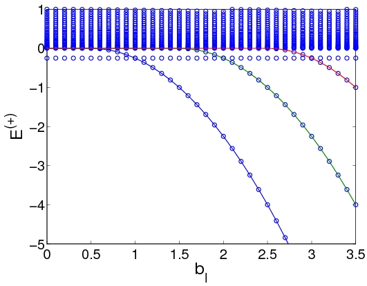
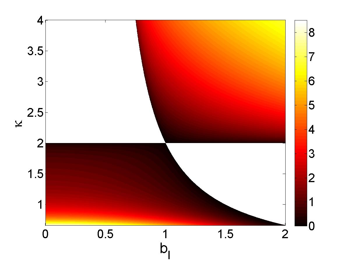
Such bound state eigenvalues only exist when . This, in turn, suggests that for the superscript potential, it will be: , i.e., all the relevant bound state eigenvalues should also emerge in the -symmetric spectrum of the potential , just as they appear in the Hermitian (real) spectrum of the potential . The only eigenvalue that will not be captured by this relation is ; see the relevant details on the spectrum of below. Furthermore, we expect that, when varying , bound state eigenvalues will emerge as crosses , , in both the spectra of .
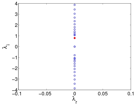
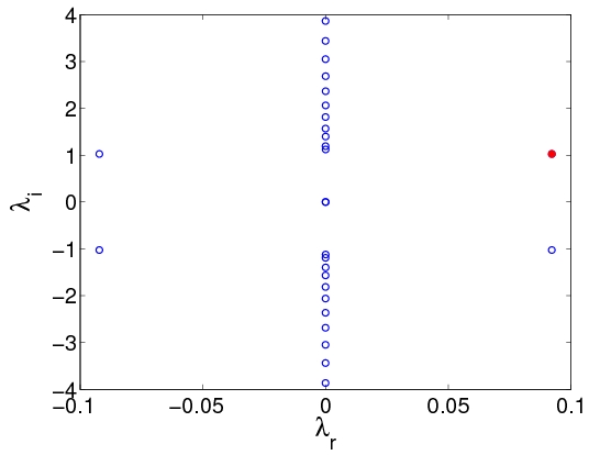
All of these conclusions are fully corroborated by the results of Fig. 1. The spectrum of considered therein turns out to be real, as may be anticipated by the -symmetry of the model, but more importantly, it turns out to be identical to that of its super-symmetric Pöschl-Teller partner, as can be seen from the theoretical lines confirming the bifurcation of the point spectrum eigenvalues at the locations theoretically predicted. Finally, indeed, the only eigenvalue that is not captured is which turns out to be invariant, under variations of . As a final note, we point out that generalizations of this potential with arbitrary coefficients in both the real and the imaginary part were considered in ahmed and the relevant -symmetric transition threshold was identified as an inequality associating the real and the imaginary part prefactors. The pertinent inequality here assumes the form and is generically satisfied (i.e., ), as can be expected by the super-symmetric partnership of the potential with a Hermitian one bearing real eigenvalues for all .
As a side remark, we observe that is invariant under . Further, both and are arbitrary real numbers and not integers. Interestingly, as shown in bagchi5 , in case is not an integer, then remarkably, the eigenvalue spectrum has two branches:
| (12) |
where , and
| (13) |
where .
From this, we infer that when and is not an integer, has two nodeless states (i.e. ) with energy eigenvalues and eigenfunctions
| (14) |
| (15) |
although the latter (as per our spectral results of Fig. 1) will only be present for . Interestingly, while for , is the ground state, but for , corresponds to the ground state.
III Nonlinear Generalization of the Model
We now turn to the corresponding nonlinear model which is the basis for the present analysis. Examining the case of the focusing nonlinearity, the operator is augmented into the nonlinear problem:
| (16) |
The most physically relevant case is that of the cubic nonlinearity , corresponding to the Kerr effect, although in recent years, examples of higher order nonlinearities (like and ) have been experimentally realized; see, e.g., for a recent example pernamb . The relevant nonlinear problem has been partially considered for in a two-parametric generalization of the potential associated with ziad2 ; see also the more recent discussions of nazari ; chen . While all of these works were restricted to the cubic case, below we will obtain exact solutions for arbitrary nonlinearity powers. Moreover, we will explain, through our -SUSY framework the existence of nonlinear dipole (and, by extension, tripole etc.) solutions identified in chen , emerging from the higher excited states of the underlying linear problem. It can be directly found that the relevant nonlinear single-hump solution for arbitrary is of the form:
| (17) |
where
| (18) |
| (19) |
and
| (20) |
Note when and , and our solution reduces to the well known solution of the NLSE with . Also note that when ,
| (21) |
which vanishes at either or the special case . Hereafter, we again restrain consideration to the special case of .
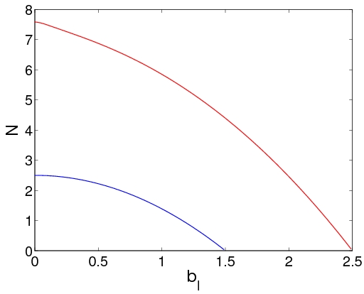
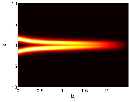
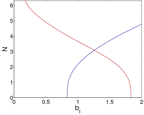
For , with , the amplitude tends to zero and the solution (17) becomes the solution of the corresponding linear limit (15) by virtue of condition (20). The solution (17) exists for when and for if . Our analytical expression only yields the trivial solution for as mentioned earlier. Notice also that when is fixed and varied, the solution tends to (14) when approaching the limit. In addition, Fig. 2 shows the dependence of norm with respect to and when the condition (20) for solution (17) is applied. The value of the norm is
| (22) |
where it has been taken into account that and is the Euler’s beta function.
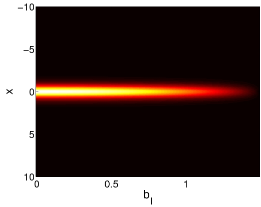
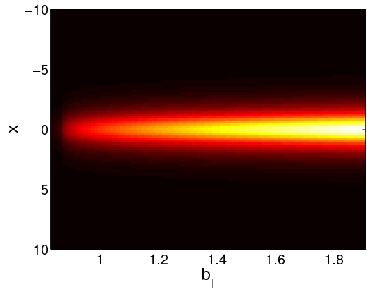
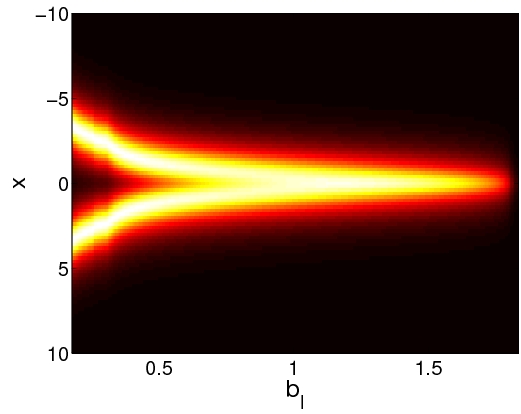
Horizontal “cuts” along the graph of Fig. 2 are shown in Figs. 3 and 4 where the continuum tendency to the linear limit (dark) is shown as a variation over for and , respectively. Apart from the analytical solution (17) which collides with the nodeless solution of the linear Schrödinger equation, we have been able to find numerically the branch that collides with the solution with a node [ in (12)-(13)]. These solutions are the generalizations (for arbitrary ) of the “dipoles” of chen . In those cases, solutions exist as long as and their monotonicity for is opposite to that of the fundamental solutions analytically identified above (hence, the above mentioned collision). Interestingly, it is worth mentioning that the latter dipole branch is present even for . In the same spirit, higher order generalizations (e.g. tripoles, quadrupoles, etc.) can also be expected in the spirit of chen , degenerating to the linear limit, respectively for , , etc.
 |
|
 |
 |
 |
|
 |
 |
We now turn to the detailed stability analysis of the relevant soliton solutions (which was not explored systematically in ziad2 ; nazari , but was touched upon in chen for ). In fact, in ziad2 a particular case example of an evolution (cf. Fig. 2 therein), as well as the positivity of the Poynting vector flux led those authors to conclude that the relevant solutions were nonlinearly stable. However, our systematic spectral stability analysis, illustrated in Figs. 5 and 7, indicates otherwise. In particular, we use a linearization ansatz of the form
| (23) |
where is the spatial profile of the standing wave solution of Eq. (17), while and correspond, respectively, to the eigenvector and eigenvalue of the linearization around the solution. The existence of eigenvalues with Re would in this (-symmetric and hence still ensuring the quartet symmetry of the relevant eigenvalues) context signal the presence of an instability.
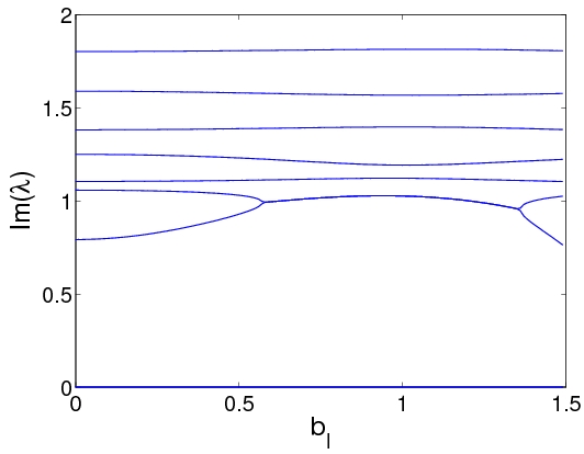
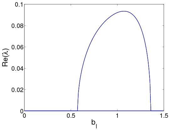
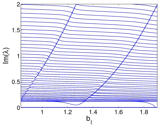
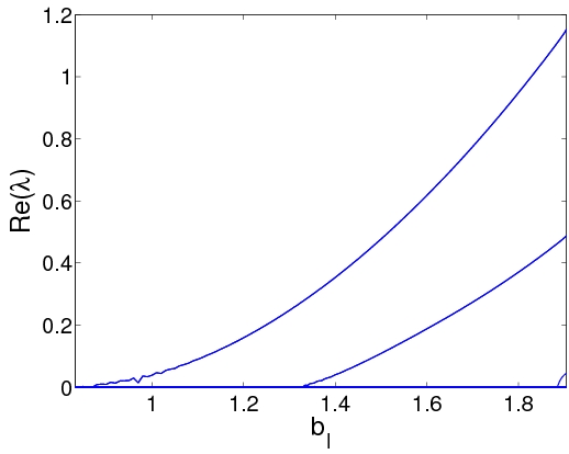
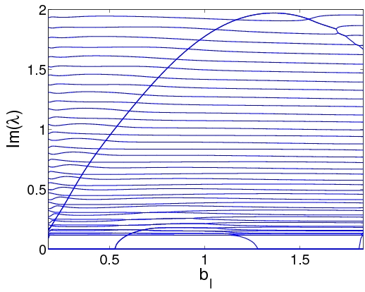
We can see in Fig. 5 that indeed such an instability is present in the interval for the nodeless solutions of . Further examination of the relevant phenomenology in Fig. 6 reveals the origin of the instability and its stark contrast with the corresponding phenomenology in the standard NLS model. In particular, the breaking of translational invariance (due to the presence of the potential) leads the corresponding neutral mode to exit along the imaginary axis of the spectral plane of the eigenvalues . However, it is well-known kks that in the standard Hamiltonian case, the relevant “internal mode” of the solitary wave associated with translation has a positive energy or signature and hence its collisions with other modes, including ones of the continuous spectrum, do not lead to instability. Here, however, as illustrated in Fig. 6 exactly the opposite occurs. As the parameter is varied, the relevant eigenvalue moves towards the continuous spectrum (whose lower limit is ) and the collision with it leads to a complex eigenvalue quartet, a feature that would never be possible for a single soliton of the regular NLS, under a translation-symmetry-breaking perturbation. This is a remarkable feature of the -symmetric NLS model that is worthy of further exploration, possibly utilizing the notion (recently discussed for -symmetric models in nixon ) of Krein signature. Notice that the work of nixon considered a case in the vicinity of the -phase transition, whereas in our setting, such a phase transition is impossible, given the real nature of the super-partner Pöschl-Teller potential, as discussed above.
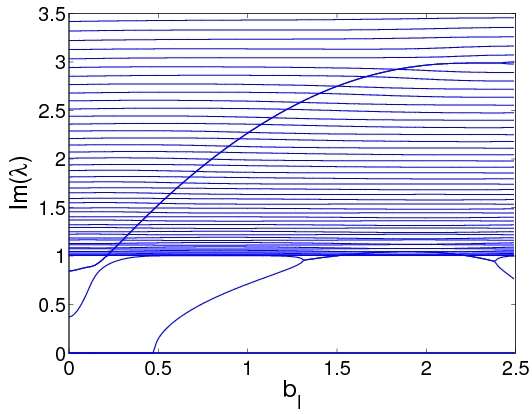
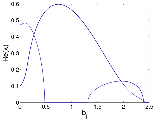
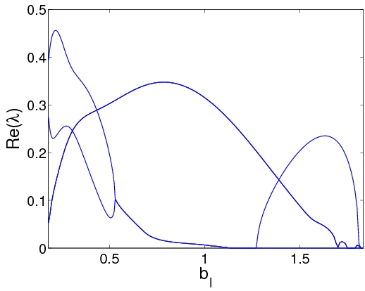
Fig. 5 shows that dipolar solutions with a single node are unstable for almost all of their existence interval expect when , i.e. in the immediate vicinity of the linear limit. There are three different instability intervals: (1) for there are two instabilities, one of exponential nature and an oscillatory one, for the oscillatory instability is the only one that persists, while the formerly real eigenmode crosses the spectral plane origin and becomes imaginary for larger . (3) for , there are two oscillatory instabilities, the previously mentioned one, and another one caused (in a way similar to the nodeless case) by the climbing up the imaginary axis of the eigenmode formerly unstable as a real pair, and its eventual collision with an eigenvalue bifurcating from the continuous spectrum.
For nodeless solutions with , we can observe in Fig. 7 (top panels) that the solution is unstable throughout its range of existence because of an eigenmode entering the phonon band and causing oscillatory instabilities; a second localized mode enters at and, finally, for , the soliton becomes exponentially unstable. Analogously, the solutions with a node are unstable for all , incurring, in fact, typically multiple instabilities for each value of the parameter, which can be summarized as follows (see the bottom panels of Fig. 7): an oscillatory instability is present for almost every value of (); apart from this we observe, for low values of , two pairs of real eigenvalues which coalesce into a quartet at ; this quartet leads to two imaginary pairs when ; one of them moves down along the imaginary axis and finally, at , an additional instability due to a real pair emerges..
It is relevant to note in passing, another interesting result which relates to the case; we have found that for , the nodeless soliton is stable for every . This, as well as the results above indicate the strong dependence of the stability properties on the precise strength of the nonlinearity parameter.
 |
 |
 |
 |
 |
 |
 |
 |
 |
 |
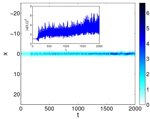
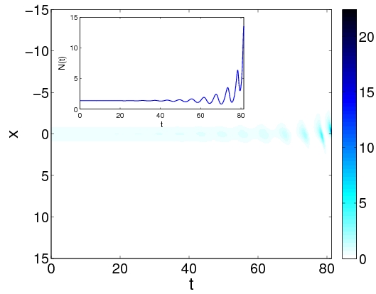
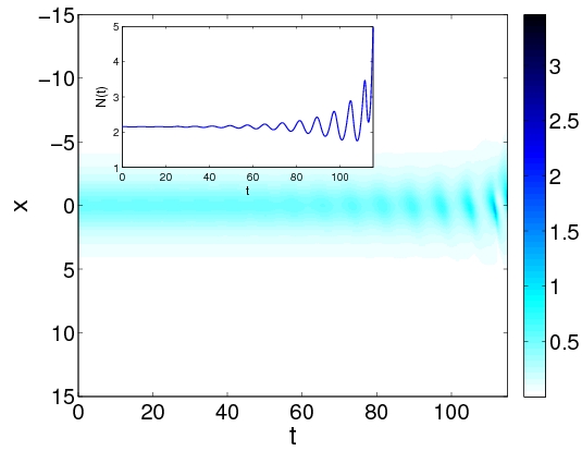
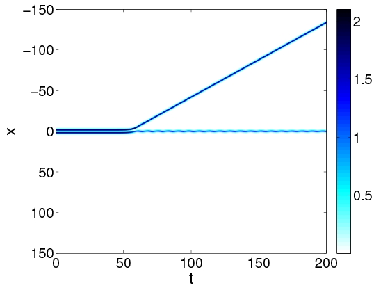
Finally, we consider the dynamics of these unstable waveforms for several prototypical cases in Fig. 8. For and we observe that when , the oscillatory (as predicted by our eigenvalue computations) nature of the instability gradually kicks in and eventually renders the solitary wave more highly localized (i.e., narrower) at and with a larger amplitude (i.e., taller). Subsequently, the amplitude of the pulse is subject to breathing, but it remains fairly robust, even after multiple collisions with small amplitude radiative wavepackets scattering back and forth from the boundaries (not visible in the scale of the plot). For and , the growth rate is larger and the instability effects stronger; it manifests in an oscillatory growth of the soliton (given the oscillatory nature of the instability), as well as a “swinging” of the solution between the gain () and loss () regions, according to the terminology of nazari . This eventually leads to rapid growth (beyond the resolution of the numerical scheme). We do not follow the solution past these large values of its amplitude. This behaviour is generic for the oscillatory instabilities as long as the growth rate is above a threshold, as shown also in the example for and , and for the nodeless and single-node solitons. Finally, we have considered the effect of the exponential instabilities in solitons with a node and . Those solitons are both exponentially and oscilatorily unstable for . In that interval, the soliton is double-humped (see Fig. 3). In the particular example of Fig. 8, we have taken where the exponential instability dominates to the oscillatory one. The dynamics here can be described as follows: the hump originally located at the loss () side shifts to and remains pinned with regular oscillations of the amplitude at . On the other hand, the hump initially at the gain () side is “ejected”, as a result of the instability, along the (exponentially localized around ) gain side of .
 |
 |
 |
 |
IV Conclusions & Future Challenges
In the present work, we revisited a potential that has been explored previously in a number of studies relating to -symmetric models. We discussed how for a special monoparametric family within this model, it is not only -symmetric but also super-symmetric with a partner which is the Pöschl-Teller potential, a feature which enabled us to identify its purely real spectrum (and the bifurcations of bound states within it) and to corroborate the corresponding results numerically. As a byproduct of its super-symmetric origin, this family of potentials was found to be devoid of a -phase-transition. We then turned to a nonlinear variant of the model for arbitrary powers of the nonlinearity, and illustrated that exact nonlinear solitonic solutions degenerated in the appropriate limit to the linear states identified previously. While there was no -phase-transition in this model, we found that the nonlinear solutions were still subject to instabilities, such as e.g. the one stemming from a collision of an internal mode with the continuous spectrum (band edge), leading to a quartet of eigenvalues. The ensuing oscillatory instability led to an oscillating, progressively larger amplitude soliton in the cases examined. Additional families of solutions were discussed, including e.g. the one-node branch (dipolar solution), and their reduced stability (in comparison to the nodeless branch) was illustrated.
While this work, to the best of our understanding, is only a first step in connecting all three notions of -symmetry, super-symmetric potentials and nonlinear phenomenology (including instabilities), naturally this is a theme that is worthy of considerable further studies. For one thing, there are numerous additional super-symmetric potentials with real spectra that can be devised and are worth examining. For instance, the sl considerations of bagchi already suggest some such options including the super-potentials or . Additionally, there have already been proposals for -symmetric square well potentials considered in the SUSY framework bagchi3 , and for non-Hermitian SUSY hydrogen-like Hamiltonians with real spectra bagchi4 . Especially in the latter higher dimensional context, understanding the delicate interplay of -symmetry, super-symmetric models with their bound states, and collapse induced by nonlinearity could be an especially interesting topic. Finally, there are some potentially intriguing deeper connections. SUSY partners are based on commutation formulae as are integrable nonlinear equations. Perhaps the latter is intrinsically responsible for the similarity of the structure of the SUSY partner potentials with the well-known Miura transformation responsible for converting the modified Korteweg-de Vries equation to the Korteweg-de Vries equation drazin . Exploring these connections further would constitute an important direction for further studies and efforts along this direction are already underway olshanii .
V Acknowledgments
This work was supported in part by the U.S. Department of Energy. AK wishes to thank Indian National Science Academy (INSA) for the award of INSA Senior Professor position at Pune University. PGK gratefully acknowledges support from NSF-DMS-1312856, the Binational Science Foundation under grant 2010239, and the ERC under FP7, Marie Curie Actions, People, International Research Staff Exchange Scheme (IRSES-605096).
References
- (1) C. M. Bender, Rep. Prog. Phys. 70, 947 (2007).
- (2) See special issues: H. Geyer, D. Heiss, and M. Znojil, Eds., J. Phys. A: Math. Gen. 39, Special Issue Dedicated to the Physics of Non-Hermitian Operators (PHHQP IV) (University of Stellenbosch, South Africa, 2005) (2006); A. Fring, H. Jones, and M. Znojil, Eds., J. Math. Phys. A: Math Theor. 41, Papers Dedicated to the Subject of the 6th International Workshop on Pseudo-Hermitian Hamiltonians in Quantum Physics (PHHQPVI) (City University London, UK, 2007) (2008); C.M. Bender, A. Fring, U. Günther, and H. Jones, Eds., Special Issue: Quantum Physics with non-Hermitian Operators, J. Math. Phys. A: Math Theor. 41, No. 44 (2012).
- (3) K. G. Makris, R. El-Ganainy, D. N. Christodoulides, and Z. H. Musslimani, Int. J. Theor. Phys. 50, 1019 (2011).
- (4) A. Ruschhaupt, F. Delgado, and J. G. Muga, J. Phys. A: Math. Gen. 38, L171 (2005).
- (5) K. G. Makris, R. El-Ganainy, D. N. Christodoulides, and Z. H. Musslimani, Phys. Rev. Lett. 100, 103904 (2008); S. Klaiman, U. Günther, and N. Moiseyev, ibid. 101, 080402 (2008); O. Bendix, R. Fleischmann, T. Kottos, and B. Shapiro, ibid. 103, 030402 (2009); S. Longhi, ibid. 103, 123601 (2009); Phys. Rev. B 80, 235102 (2009); Phys. Rev. A 81, 022102 (2010).
- (6) A. Guo, G. J. Salamo, D. Duchesne, R. Morandotti, M. Volatier-Ravat, V. Aimez, G. A. Siviloglou, and D. N. Christodoulides, Phys. Rev. Lett. 103, 093902 (2009); C. E. Rüter, K. G. Makris, R. El-Ganainy, D. N. Christodoulides, M. Segev, and D. Kip, Nature Phys. 6, 192 (2010); A. Regensburger, C. Bersch, M.-A. Miri, G. Onishchukov, D. N. Christodoulides, and U. Peschel, Nature 488, 167 (2012).
- (7) J. Schindler, A. Li, M.C. Zheng, F.M. Ellis, and T. Kottos, Phys. Rev. A 84, 040101 (2011).
- (8) J. Schindler, Z. Lin, J. M. Lee, H. Ramezani, F. M. Ellis, and T. Kottos, J. Phys. A: Math. Theor. 45, 444029 (2012).
- (9) C. M. Bender, B. Berntson, D. Parker, and E. Samuel Am. J. Phys. 81, 173 (2013).
- (10) B. Peng, S.K. Özdemir, F. Lei, F. Monifi, M. Gianfreda, G.L. Long, S. Fan, F. Nori, C.M. Bender and L. Yang, arXiv: 1308.4564.
- (11) F. Cooper, A. Khare, U. Sukhatme, Supersymmetry in quantum mechanics, World Scientific (Singapore, 2002).
- (12) M. Ali Miri, M. Heinrich, R. El-Ganainy and D.N. Christodoulides, Phys. Rev. Lett. 110, 233902 (2013); M. Heinrich, M. Ali Miri, S. Stützer, R. El-Ganainy, S. Nolte, A. Szameit and D.N. Christodoulides, Nat. Comm. 5, 3698 (2014).
- (13) M. Ali Miri, M. Heinrich and D.N. Christodoulides, Phys. Rev. A 87, 043819 (2013).
- (14) Z. Lin, H. Ramezani, T. Eichelkraut, T. Kottos, H. Cao and D. Christodoulides, Phys. Rev. Lett. 106, 213901 (2011).
- (15) B. Midya, Physical Review A 89, 032116 (2014).
- (16) G. Poschl, E. Teller, Z. Phys. 83, 143 (1933).
- (17) L. D. Landau and E. M. Lifshitz, Quantum Mechanics (Moscow: Nauka publishers, 1989).
- (18) B. Bagchi, S. Mallik and C. Quesne, Int. J. Mod. Phys. A 16, 2859 (2001).
- (19) B. Bagchi and R. Roychoudhury, J. Phys. A 33, L1 (2000).
- (20) Z. Ahmed, Phys. Lett. A 282, 343 (2001).
- (21) B. Bagchi and C. Quesne, Phys. Lett. A 273, 285 (2000).
- (22) A.S. Reyna and C.B. de Araújo Phys. Rev. A 89, 063803 (2014); A.S. Reyna, K.C. Jorge, and C.B. de Araújo Phys. Rev. A 90, 063835 (2014).
- (23) Z. H.Musslimani, K. G. Makris, R. El-Ganainy and D. N. Christodoulides, Phys. Rev. Lett. 100, 030402 (2008).
- (24) M. Nazari, F. Nazari, and M. K. Moravvej-Farshi, J. Opt. Soc. Am. B 29, 3057 (2012).
- (25) H. Chen, S. Hu and L. Qi, Opt. Commun. 331, 139 (2014).
- (26) T. Kapitula, P.G. Kevrekidis, B. Sandstede, Physica D 195 263 (2004).
- (27) S. Nixon, J. Yang, arXiv:1506.04445.
- (28) B. Bagchi, S. Mallik, C. Quesne, Mod. Phys. Lett. A 17, 1651 (2002).
- (29) O. Rosas-Ortiz and R. Muñoz, J. Phys. A 36, 8497 (2003).
- (30) P.G. Drazin, R.S. Johnson, Solitons: An Introduction, Cambridge University Press (Cambridge, 1989).
- (31) A. Koller and M. Olshanii, Phys. Rev. E 84, 066601 (2011).