A generalised Airy distribution function for the accumulated area swept by $N$ vicious Brownian paths

Abstract

In this work exact expressions for the distribution function of the accumulated area swept by reunions and meanders of $N$ vicious Brownian particles up to time $T$ are derived. The results are expressed in terms of a generalised Airy distribution function, containing the Vandermonde determinant of the Airy roots. By mapping the problem to an Random Matrix Theory ensemble we are able to perform Monte Carlo simulations finding perfect agreement with the theoretical results.

1 Introduction

Since the seminal work of de Gennes on simple models of fibrous structures and its popularisation by Fisher, the study of vicious walkers (namely, walkers that do not intersect) have attracted attention during the last two decades due to the wide range of applications in various branches of science and their connections to random matrix theory Forrester2011 ; Schehr2013 ; Baik2000 ; Forrester2001 ; Johansson2003 ; Nagao2003 ; Katori2004 ; Ferrari2005 ; Tracy2007 ; Daems2007 ; Schehr2008 ; Novak2009 ; Nadal2009 ; Rambeau2010 ; Borodin2010 ; Bleher2011 ; Adler2012 . Similarly, the statistical properties of the area swept by a Brownian excursion is a problem that was originally studied by mathematicians. The Laplace transform of the distribution of the area (known as the Airy distribution function) was first computed by Darling and Louchard Darling1983 ; Louchard1984 . The derivation of its moments together with the actual distribution were obtained by Takács Takacs1991 ; Takacs1993 ; Takacs1995 . The Airy distribution function has appeared in a number of problem from different areas from graph theory and computer science as well as in physical systems modelling one dimensional fluctuating interfaces Majumdar2004 ; Majumdar2005 , applications in laser cooling Barkai2014 ; Kessler2014 and fluctuations of sizes of ring polymers Medalion2015 .

In this work, we focus on obtaining exact expressions for the accumulated area swept by $N$ vicious Brownian motions. This paper is organised as follows: in section 2, we define the process of vicious walkers and the stochastic quantities we are interested in. In particular, we show in section 3 that the Laplace transform of PDF of the accumulated area can be expressed as a ratio of two N-particle propagators, which can be constructed as Slater determinants of single-particle states. This is a straightforward consequence of using Quantum Mechanics formalism or, alternatively, of the Karlin-McGregor formula. The resulting expression is fairly general. In order to extract some properties we consider two type of processes: reunions and meanders. Moreover we consider two type of boundary conditions at $x=0$: absorbing boundary conditions (section 4) and reflecting boundary conditions (section 5). The inverse Laplace transform is resolved in section 6 and a formula for its negative moments is obtained in section 7. Finally, in section 8, using a mapping between processes of vicious walkers to ensembles of Random Matrix Theory we are able to perform Monte Carlo simulations and compare with the exact formulas obtained in the previous sections.

2 Model definitions

Consider the set of trajectories defined by $N$ one-dimensional Brownian particles $\bm{x}(\tau)=(x_{1}(\tau),\ldots,x_{N}(\tau))$ with $\tau\in[0,T]$ such that $0<x_{1}(\tau)<\cdots<x_{N}(\tau)$ and let us denote as $\mathcal{M}_{N}[\bm{x}(\tau)]$ its probability measure. Next, let us define as $A_{i}$ the area swept by particle $i$:

$$\begin{split}A_{i}=\int_{0}^{T}x_{i}(\tau)d\tau\,.\end{split}$$

The set of areas $\bm{A}=(A_{1},\ldots,A_{N})$ is a random $N$-tuple whose joint PDF (jPDF) is given by viz.

$$\begin{split}\mathcal{P}_{N}(\bm{A},T)=\int_{\bm{x}(0)=\bm{x}_{i}}^{\bm{x}(T)=\bm{x}_{f}}\mathcal{D}\bm{x}(\tau)\mathcal{M}_{N}[\bm{x}(\tau)]\prod_{i=1}^{N}\delta\left(\int_{0}^{T}x_{i}(\tau)d\tau-A_{i}\right)\,.\end{split}$$ (1)

Notice that the jPDF (1) contains the PDF of the area swept for each curve $i=1,\ldots,N$

$$\begin{split}\mathcal{P}^{(i)}_{N}(A_{i},T)=\int_{0}^{\infty}\cdots\int_{0}^{\infty}dA_{1}\cdots dA_{i-1}dA_{i+1}\cdots dA_{N}\mathcal{P}_{N}(\bm{A},T)\,,\end{split}$$ (2)

and, in particular, the PDFs of the area for the bottom and top curves denoted as $\mathcal{T}_{N}(A,T)\equiv\mathcal{P}^{(N)}_{N}(A,T)$ and $\mathcal{B}_{N}(A,T)\equiv\mathcal{P}^{(1)}_{N}(A,T)$, respectively. It also contains the PDF of the total area, defined as

$$\begin{split}\mathcal{S}_{N}(A,T)=\int_{0}^{\infty}\cdots\int_{0}^{\infty}dA_{1}\cdots dA_{N}\mathcal{P}_{N}(\bm{A},T)\delta\left(A-\sum_{i=1}^{N}A_{i}\right)\,.\end{split}$$ (3)

In this work we present exact formulas for the PDF $\mathcal{S}_{N}(A,T)$ for the accumulated area and compare the expressions with Monte Carlo simulations. A thorough analysis based on Monte Carlo simulations on the marginals $\mathcal{P}^{(i)}_{N}(A,T)$ for $i=1,\ldots,N$ will be discussed somewhere else.

3 Path Integral Approach

Combining (1) and (3) yields

$$\begin{split}\mathcal{S}_{N}(A,T)=\int_{\bm{x}(0)=\bm{x}_{i}}^{\bm{x}(T)=\bm{x}_{f}}\mathcal{D}\bm{x}(\tau)\mathcal{M}_{N}[\bm{x}(\tau)]\delta\left(A-\sum_{i=1}^{N}\int_{0}^{T}x_{i}(\tau)d\tau\right)\,,\end{split}$$

with

$$\begin{split}\mathcal{M}[\bm{x}(\tau)]=\frac{1}{Z}\exp\left[-\frac{1}{2}\sum_{i=1}^{N}\int_{0}^{T}d\tau\left(\frac{dx_{i}(\tau)}{d\tau}\right)^{2}\right]C_{N}[\bm{x}(\tau)]\,,\end{split}$$

where $Z$ is the normalisation factor and $C_{N}[\bm{x}(\tau)]$ is an indicator function imposing the constraint of vicious particles $0<x_{1}(\tau)<\cdots<x_{N}(\tau)$ on the positive part of the real line. Further, the Laplace transform of $\mathcal{S}_{N}(A,T)$,

$$\begin{split}\widehat{\mathcal{S}}_{N}(\lambda,T)=\left\langle e^{-\lambda A}\right\rangle_{\mathcal{S}_{N}}\equiv\int_{0}^{\infty}dA~{}\mathcal{S}_{N}(A,T)e^{-\lambda A}\end{split}$$

has the following representation using path integral approach:

$$\begin{split}\widehat{\mathcal{S}}_{N}(\lambda,T)&=\int^{\bm{x}(T)=\bm{x}_{f}}_{\bm{x}(0)=\bm{x}_{i}}\mathcal{D}\bm{x}(\tau)\mathcal{M}_{N}[\bm{x}(\tau)]\exp\left[-\lambda\sum_{i=1}^{N}\int_{0}^{T}x_{i}(\tau)d\tau\right]\,.\end{split}$$ (4)

In Quantum Mechanics formalism, the expression (4) can be expressed as the ratio of two propagators

$$\begin{split}\widehat{\mathcal{S}}_{N}(\lambda,T)&=\frac{G^{(1)}_{N}(\bm{x}_{f},T|\bm{x}_{i},0)}{G_{N}^{(0)}(\bm{x}_{f},T|\bm{x}_{i},0)}\,,\end{split}$$ (5)

with $G^{(a)}_{N}(\bm{x},T|\bm{x}_{0},0)=\left\langle\bm{x}|e^{-H^{(a)}_{N}T}|\bm{x}_{0}\right\rangle$ and Hamiltonian operators

$$\begin{split}H^{(a)}_{N}=\sum_{j=1}^{N}h_{j}^{(a)}=-\frac{1}{2}\sum_{j=1}^{N}\partial_{x_{j}}^{2}+\sum_{j=1}^{N}V^{(a)}(x_{j})\,,\quad\quad a=0,1\end{split}$$ (6)

and $V^{(0)}(x)$ a confining potential in $\mathbb{R}^{+}$, while $V^{(1)}(x)=\lambda x$ for $x>0$ and infinity for $x\leq 0$. Besides, Brownian particles are not allowed to cross which in QMf corresponds to having fermions. Considering the latter and that the potentials are one-particle type operators, the eigenfunctions of $H^{(a)}_{N}$ are given by the Slater determinant of the eigenfunctions corresponding to the one-particle problem $h^{(a)}$, that is

$$\begin{split}G_{N}^{(a)}(\bm{y},T|\bm{x},0)&=\sum_{\bm{n}}\Phi^{(a)}_{\bm{n}}(\bm{y})\overline{\Phi}^{(a)}_{\bm{n}}(\bm{x})e^{-E^{(a)}_{\bm{n}}T}\,,\end{split}$$ (7)

with

$$\begin{split}\Phi^{(a)}_{\bm{n}}(\bm{x})=\frac{1}{\sqrt{N!}}\det_{1\leq i,j\leq N}\phi^{(a)}_{n_{i}}(x_{j})\,,\quad\quad E^{(a)}_{\bm{n}}=\sum_{i=1}^{N}e^{(a)}_{n_{i}}\,,\quad\quad h^{(a)}\left|\phi^{(a)}_{n}\right\rangle=e^{(a)}_{n}\left|\phi^{(a)}_{n}\right\rangle\,.\end{split}$$

Once the corresponding one-particle problems of the numerator and denominator have been solved, we have solved the problem via the formula (5). However, the corresponding expression is still too general to extract general mathematical properties. Thus, in light of the previous work we will particularise (5) to the cases of reunions and meanders.
For reunions we mean the set of processes by which the $N$ vicious Brownian paths start and finish at the same point, that is $\bm{x}_{i}=\bm{x}_{f}=\bm{0}$. This is achieved by taking $\bm{x}_{i}=\bm{x}_{f}=\bm{\epsilon}$ with $\bm{\epsilon}=(\epsilon_{1},\cdots,\epsilon_{N})$, and taking the limit $\bm{\epsilon}$ to $\bm{0}$, viz.

$$\begin{split}\widehat{\mathcal{S}}^{(r)}_{N}(\lambda,T)&=\lim_{\bm{\epsilon}\to\bm{0}}\frac{G^{(1)}_{N}(\bm{\epsilon},T|\bm{\epsilon},0)}{G_{N}^{(0)}(\bm{\epsilon},T|\bm{\epsilon},0)}\,.\end{split}$$ (8)

For meanders we mean the set of processes where the paths start at $\bm{x}_{i}=\bm{0}$ and are allowed to finish at any final position $\bm{x}_{f}$ at time $T$. As such we need to integrate over all possible final positions and, therefore, the Laplace transform of the corresponding PDF reads

$$\begin{split}\widehat{\mathcal{S}}^{(m)}_{N}(\lambda,T)=\lim_{\bm{\epsilon}\to\bm{0}}\frac{\int_{\bm{W}_{N}}d^{N}\bm{x}_{f}~{}G^{(1)}_{N}(\bm{x}_{f},T|\bm{\epsilon},0)}{\int_{\bm{W}_{N}}d^{N}\bm{x}_{f}~{}G_{N}^{(0)}(\bm{x}_{f},T|\bm{\epsilon},0)}\,,\end{split}$$ (9)

where $\bm{W}_{N}$ stands for the Weyl chamber $\bm{W}_{N}=\left\{\bm{x}\in\mathbb{R}^{N}|0\leq x_{1}\leq\cdots\leq x_{N}\right\}$ and $d^{N}\bm{x}=dx_{1}\cdots dx_{N}$.

4 Absorbing Boundary conditions

We note in the two cases above that we will need the one-particle problem for $a=1$ (the one-particle problem for $a=0$ is treated in the appendices). For absorbing boundary conditions (i.e. the corresponding eigenfunctions of the one-particle problem obey $\phi(x=0)=0$) it has the well-known solution

$$\begin{split}\phi^{(1)}_{n}(x)=\frac{\sqrt{(2\lambda)^{1/3}}}{|\text{Ai}^{\prime}(-\alpha_{n})|}\text{Ai}[(2\lambda)^{1/3}x-\alpha_{n}]\,,\quad e^{(1)}_{n}=\alpha_{n}\lambda^{2/3}2^{-1/3}\,,\quad\quad n=1,2,\ldots\end{split}$$

where $\text{Ai}(x)$ is the Airy function with zeros $z=-\alpha_{n}$ with $n\in\{1,2,\ldots\}$. Thus the eigenfunction for the $N$-particle problem is:

$$\begin{split}\Phi^{(1)}_{\bm{n}}(\bm{x})&=\frac{1}{\sqrt{N!}}\det_{1\leq i,j\leq N}\phi^{(1)}_{n_{i}}(x_{j})=\frac{(2\lambda)^{N/6}}{\sqrt{N!}\prod_{i=1}^{N}|\text{Ai}^{\prime}(-\alpha_{n_{i}})|}\det_{1\leq i,j\leq N}\left[\varphi_{n_{i}}(z_{j})\right]\,,\end{split}$$ (10)

where we have defined $\varphi_{n}(z)=\text{Ai}(z-\alpha_{n})$ with $z=(2\lambda)^{1/3}x$.

4.1 Reunions

To obtain an exact expression for $\widehat{\mathcal{S}}^{(r)}_{N}(\lambda,T)$ given by (8) we need to perform the Taylor expansion of the Slater determinant (10) containing the Airy eigenfunctions. To do so we make use of the following formula Laurenzi2011 :

$$\begin{split}\text{Ai}(t)\text{Bi}(z+t)-\text{Bi}(t)\text{Ai}(z+t)=\frac{1}{\pi}\sum_{\ell=0}^{\infty}\frac{z^{\ell}}{\ell!}Q_{\ell}(t)\,,\end{split}$$

with $Q_{n}(z)$ the Abramochkin polynomials Laurenzi2011 . In our case, we take that $t=-\alpha_{n}$ which yields

$$\begin{split}\text{Ai}(z-\alpha_{n})=\text{Ai}^{\prime}(-\alpha_{n})\sum_{\ell=0}^{\infty}\frac{z^{\ell}}{\ell!}Q_{\ell}(-\alpha_{n})\,,\end{split}$$

where we have used the identity $\pi\text{Bi}(-\alpha_{n})\text{Ai}^{\prime}(-\alpha_{n})=-1$. Combining this together with the standard formula of the Taylor series of a Slater determinant (see appendix A), we arrive at

$$\begin{split}\det_{1\leq i,j\leq N}\varphi_{n_{i}}(z_{j})&=\left[\prod_{j=1}^{N}\text{Ai}^{\prime}(-\alpha_{n_{j}})\right]\sum_{\bm{\ell}\in U_{N}}\frac{(2\lambda)^{\frac{1}{3}\sum_{j=1}^{N}\ell_{j}}}{\ell_{1}!\cdots\ell_{N}!}\det_{1\leq i,j\leq N}[x^{\ell_{j}}_{i}]\det_{1\leq i,j\leq N}[Q_{\ell_{i}}(-\alpha_{n_{j}})]\,,\end{split}$$ (11)

where $\bm{\ell}\in U_{N}$ stands for the sum over all ordered $N$-tuple indices $\bm{\ell}=(\ell_{1},\ldots,\ell_{N})$, that is with $\ell_{1}<\ell_{2}<\cdots<\ell_{N}$.
Everything boils down to be able to find an expression for the determinant $\det_{1\leq i,j\leq N}[Q_{\ell_{i}}(-\alpha_{n_{j}})]$ of the Abramochkin polynomials evaluated at the Airy roots. It turns out that it is possible to obtain the lowest contribution in $\bm{\epsilon}$ if we recall that the odd-numbered polynomials are such that $Q_{2n+1}(z)=z^{n}+\text{lower order terms}$, while even-numbered polynomials can be expressed in terms of the previous odd-numbered ones. This automatically implies that the first non-zero lowest-order contribution in $\bm{\epsilon}$ in the sum in eq. (11) is given by taking $\ell_{j}=2(j-1)+1$ for $j=1,\ldots,N$. This eventually yields:

$$\begin{split}\det_{1\leq i,j\leq N}\varphi_{n_{i}}(z_{j})&\sim(2\lambda)^{\frac{N^{2}}{3}}\left[\prod_{j=1}^{N}\text{Ai}^{\prime}(-\alpha_{n_{j}})\right]\left[\prod_{i=1}^{N}x_{i}\right]\Delta_{N}(x_{1}^{2},\ldots x_{N}^{2})\Delta_{N}(\alpha_{n_{1}},\dots\alpha_{n_{N}})\,,\end{split}$$ (12)

where we have defined $\gamma_{N}=(-1)^{\frac{N(N-1)}{2}}/[1!\cdots(2N+1)!]$, and $\Delta_{N}(a_{1},\ldots,a_{N})$ is the Vandermonde determinant:

$$\begin{split}\Delta_{N}(a_{1},\ldots,a_{N})\equiv\begin{vmatrix}1&\cdots&1\\ a_{1}&\cdots&a_{N}\\ \vdots&\ddots&\vdots\\ a_{1}^{N-1}&\cdots&a_{N}^{N-1}\\ \end{vmatrix}=\prod_{1\leq i<j\leq N}(a_{i}-a_{j})\,.\end{split}$$

To obtain the expression (12) we have used that

$$\begin{split}\det_{1\leq i,j\leq N}[x^{2(j-1)+1}_{i}]&=\left[\prod_{i=1}^{N}x_{i}\right]\Delta_{N}(x_{1}^{2},\ldots x_{N}^{2})\,,\quad\det_{1\leq i,j\leq N}[Q_{\ell_{i}}(-\alpha_{n_{j}})]=(-1)^{\frac{N(N-1)}{2}}\Delta_{N}(\alpha_{n_{1}},\dots\alpha_{n_{N}})\,.\end{split}$$

The final expression of the Taylor expansion for the $N$-particle eigenfunction is:

$$\begin{split}\Phi^{(1)}_{\bm{n}}(\bm{\epsilon})&\sim\beta_{N}(2\lambda)^{\frac{N(2N+1)}{6}}\left[\prod_{j=1}^{N}\frac{\text{Ai}^{\prime}(-\alpha_{n_{j}})}{|\text{Ai}^{\prime}(-\alpha_{n_{j}})|}\right]\left[\prod_{i=1}^{N}\epsilon_{i}\right]\Delta_{N}(\epsilon_{1}^{2},\ldots\epsilon_{N}^{2})\Delta_{N}(\alpha_{n_{1}},\dots\alpha_{n_{N}})\,,\end{split}$$ (13)

with $\beta_{N}=\gamma_{N}/\sqrt{N!}$. A similar derivation can be done for the denominator (see appendix B). Using the results (13), (30), and (39) in the corresponding expression (7) of the propagator, and after rearranging terms, we eventually obtain the Laplace transform of the PDF $\mathcal{S}^{(r)}_{N}(A,T)$, viz.

$$\begin{split}\widehat{\mathcal{S}}^{(r)}_{N}(\lambda,T)&=\frac{\left(\lambda T^{3/2}\right)^{E^{(r)}_{N}}}{A^{(r)}_{N}}\sum_{n_{1},\ldots,n_{N}}\Delta^{2}_{N}(\alpha_{n_{1}},\dots\alpha_{n_{N}})e^{-(\lambda T^{3/2})^{2/3}2^{-1/3}\sum_{i=1}^{N}\alpha_{n_{i}}}\,,\\ A^{(r)}_{N}&=\frac{2^{\frac{1}{2}E_{N}^{(r)}}}{\pi^{N}}\prod_{j=0}^{N-1}\Gamma(2+j)\Gamma(3/2+j)\,,\quad\quad E^{(r)}_{N}=\frac{1}{3}N(2N+1)\,.\end{split}$$ (14)

4.2 Meanders

For the case (9) we report the final result (the derivation can be found in appendix C)

$$\begin{split}\widehat{\mathcal{S}}^{(m)}_{N}(\lambda,T)&=\frac{\left(\lambda T^{3/2}\right)^{E^{(m)}_{N}}}{A^{(m)}_{N}}\sum_{n_{1},\ldots,n_{N}}B^{(A)}_{N}(\alpha_{n_{1}},\ldots,\alpha_{n_{N}})\Delta_{N}(\alpha_{n_{1}},\dots\alpha_{n_{N}})e^{-(\lambda T^{3/2})^{2/3}2^{-1/3}\sum_{i=1}^{N}\alpha_{n_{i}}}\,,\end{split}$$ (15)

where

$$\begin{split}B^{(A)}_{N}(\alpha_{n_{1}},\ldots,\alpha_{n_{N}})&=\frac{1}{\prod_{i=1}^{N}\text{Ai}^{\prime}(-\alpha_{n_{i}})}\int_{\bm{W}_{N}}d^{N}\bm{x}\det_{1\leq i,j\leq N}\left[\text{Ai}(x_{j}-\alpha_{n_{i}})\right]\,,\quad E^{(m)}_{N}=\frac{N^{2}}{3}\,.\end{split}$$

In this case we were unable to find a simple expression for the normalisation constant $A_{N}^{(m)}$.

5 Reflecting boundary conditions

So far we have preoccupied ourselves by considering absorbing boundary conditions at $x=0$. We have also considered how the preceding derivations change when we take reflecting boundary conditions instead. Apart from the mathematical curiosity, the resulting process is interesting as it is related to the work Katori2004 for processes $\bm{X}^{(-1/2,0)}(t)$ which show a transition from type D to type D’ matrix ensembles (see Katori2004 for details).
The first thing is to notice how the one-particle wave-function changes in this case. If we denote as $z=-\beta_{n}$ with $n\in{1,2,\ldots}$ the zeros of the derivative of the Airy function $\text{Ai}^{\prime}(x)$, then

$$\begin{split}\phi_{n}^{(1)}(x)=\frac{\sqrt{(2\lambda)^{1/3}}}{\sqrt{\beta_{n}}|\text{Ai}(-\beta_{n})|}\text{Ai}((2\lambda)^{1/3}x-\beta_{n})\,,\quad\quad e^{(1)}_{n}=\beta_{n}\lambda^{2/3}2^{-1/3}\end{split}$$

Thus, in this case the $N$-particle wavefunction takes the following form:

$$\begin{split}\Psi^{(1)}_{\bm{n}}(\bm{x})=\frac{(2\lambda)^{N/6}}{\sqrt{N!}\prod_{i=1}^{N}\sqrt{\beta_{n_{i}}}|\text{Ai}(-\beta_{n_{i}})|}\det_{1\leq i,j\leq N}[\psi_{n_{i}}(z_{j})]\,,\quad\quad\psi_{n}(z)=\text{Ai}(z-\beta_{n})\,,\quad z=(2\lambda)^{1/3}x\,.\end{split}$$

5.1 Reunions

We are left with deriving a Taylor expansion of the Slater determinant, as before. In this case, the other Abramochkin polynomials Laurenzi2011 become useful:

$$\begin{split}\text{Bi}^{\prime}(z)\text{Ai}(z+t)-\text{Ai}^{\prime}(z)\text{Bi}(z+t)=\frac{1}{\pi}\sum_{n=0}^{\infty}\frac{t^{n}}{n!}P_{n}(z)\,.\end{split}$$

From this expression we choose $t=-\beta_{n}$ to write

$$\begin{split}\text{Ai}(z-\beta_{n})=\text{Ai}(-\beta_{n})\sum_{\ell=0}^{\infty}\frac{t^{\ell}}{\ell!}P_{\ell}(-\beta_{\ell})\,,\end{split}$$

where we have used the property $\pi\text{Bi}^{\prime}(-\beta_{n})\text{Ai}(-\beta_{n})=1$. The expansion of the Slater determinant yields

$$\begin{split}\det_{1\leq i,j\leq N}\psi_{n_{i}}(z_{j})&=\left[\prod_{j=1}^{N}\text{Ai}(-\beta_{n_{j}})\right]\sum_{\bm{\ell}\in U_{N}}\frac{(2\lambda)^{\frac{1}{3}\sum_{j=1}^{N}\ell_{j}}}{\ell_{1}!\cdots\ell_{N}!}\det_{1\leq i,j\leq N}[x^{\ell_{j}}_{i}]\det_{1\leq i,j\leq N}[P_{\ell_{i}}(-\beta_{n_{j}})]\,,\end{split}$$

Again here, the lowest contribution in $\bm{\epsilon}$ is given by the even-labelled polynomials $P_{2n}(z)=z^{n}+\cdots$ for $n=0,1,2\ldots$ and with $P_{0}(z)=1$. Thus we must take $\ell_{j}=2(j-1)$ for $j=1,\ldots,N$ yielding the following result for the Slater determinant

$$\begin{split}\Psi^{(1)}_{\bm{n}}(\bm{\epsilon})=\delta_{N}(2\lambda)^{\frac{N(2N-1)}{6}}\left[\prod_{j=1}^{N}\frac{\text{Ai}(-\beta_{n_{j}})}{\sqrt{\beta_{n_{j}}}|\text{Ai}(-\beta_{n_{j}})|}\right]\Delta_{N}(x_{1}^{2},\ldots,x_{N}^{2})\Delta_{N}(\beta_{n_{1}},\ldots,\beta_{n_{N}})\end{split}$$

with $\delta_{N}=(-1)^{\frac{N(N-1)}{2}}/[0!2!\cdots 2(N-1)!\sqrt{N!}]$. A similar analysis can be done to the propagator in the denominator of eq. (5) (see appendix B) eventually obtaining

$$\begin{split}\widehat{\mathcal{S}}^{(r,R)}_{N}(\lambda,T)&=\frac{\left(\lambda T^{3/2}\right)^{E^{(r)}_{N}}}{A^{(r)}_{N}}\sum_{n_{1},\ldots,n_{N}}\frac{\Delta^{2}_{N}(\beta_{n_{1}},\dots,\beta_{n_{N}})}{\beta_{n_{1}}\cdots\beta_{n_{N}}}e^{-(\lambda T^{3/2})^{2/3}2^{-1/3}\sum_{i=1}^{N}\beta_{n_{i}}}\\ A^{(r)}_{N}&=\frac{2^{\frac{1}{2}E^{(r)}_{N}}}{\pi^{N}}\prod_{j=0}^{N-1}\Gamma\left(\frac{1}{2}+j\right)\Gamma\left(j+2\right)\,,\quad\quad E^{(r)}_{N}=\frac{1}{3}N(2N-1)\,,\quad\quad\end{split}$$

5.2 Meanders

Similarly, in the case of meanders (see appendix C), we obtain

$$\begin{split}\widehat{\mathcal{S}}^{(m)}_{N}(\lambda,T)&=\frac{\left(\lambda T^{3/2}\right)^{E^{(m,R)}_{N}}}{A^{(m)}_{N}}\sum_{n_{1},\ldots,n_{N}}B^{(R)}_{N}(\beta_{n_{1}},\ldots,\beta_{n_{N}})\frac{\Delta_{N}(\beta_{n_{1}},\dots\beta_{n_{N}})}{\beta_{n_{1}}\cdots\beta_{n_{N}}}e^{-(\lambda T^{3/2})^{2/3}2^{-1/3}\sum_{i=1}^{N}\beta_{n_{i}}}\,,\end{split}$$ (16)

where

$$\begin{split}B^{(R)}_{N}(\beta_{n_{1}},\ldots,\beta_{n_{N}})&=\frac{1}{\prod_{i=1}^{N}\text{Ai}(-\beta_{n_{i}})}\int_{\bm{W}_{N}}d^{N}\bm{x}\det_{1\leq i,j\leq N}\left[\text{Ai}(x_{j}-\beta_{n_{i}})\right]\,,\quad E^{(m)}_{N}=\frac{1}{3}N(N-1)\,.\end{split}$$

and with no simple expression for the normalisation constant $A^{(m)}_{N}$.

6 Inverse Laplace transform of $\widehat{\mathcal{S}}_{N}(\lambda,T)$

First of all, we start by noticing that $\widehat{\mathcal{S}}_{N}(\lambda,T)=\widehat{\mathcal{Q}}_{N}(s)$ with $s=\lambda T^{3/2}$. This, as pointed out already in Majumdar2005 , implies a scaling law of the form $\mathcal{S}_{N}(A,T)=T^{-3/2}\mathcal{Q}_{N}(AT^{-3/2})$ so that $\widehat{\mathcal{Q}}_{N}(s)=\mathcal{L}[\mathcal{Q}_{N}(x)]$ with $x=AT^{-3/2}$. This applies to both cases of reunions and meanders. Notice that, even though this scaling appears mathematically, it can be easily derived by simple dimensional analysis. Indeed, as the dimensions of the diffusion constant are $[D]=L^{2}T^{-1}$ and the dimensions of area in our problem are $[A]=LT$ (Nb. here our $T$ refers to the time dimension, not to be confused with our final time $T$) then we have that

$$\begin{split}\mathcal{S}_{N}(A,T)=\frac{1}{\sqrt{DT^{3}}}\mathcal{Q}_{N}\left(\frac{A}{\sqrt{DT^{3}}}\right)\,,\end{split}$$

as we have found. Secondly, by looking at the exponents $E_{N}^{(r)}$ and $E_{N}^{(m)}$ (see either at table 1 or the expressions for the exponents in eqs. (14) and (16)), it is clear that we must perform the inverse Laplace transform $\mathcal{L}^{-1}[s^{\delta}e^{s^{2/3}}]$ with $\delta$ either an integer or one-third of an integer.
To this end, we start from the result

$$\begin{split}\int_{0}^{\infty}F(x)e^{-sx}dx=e^{-s^{2/3}}\,,\quad F(x)=2^{1/3}J(2^{1/3}x^{-2/3})x^{-5/3}\,,\end{split}$$

with

$$\begin{split}J(x)=\frac{2^{2/3}x}{3^{3/2}\sqrt{\pi}}U(1/6,4/3,2x^{3}/27)e^{-\frac{2x^{3}}{27}}\,,\end{split}$$

and with $U(a,b,x)$ the confluent hypergeometric function. After doing the rescalling of $s^{2/3}\to 2^{-1/3}\gamma s^{2/3}$, and a change of variables, we obtain the following formula

$$\begin{split}s^{n+2k/3}e^{-\gamma 2^{-1/3}s^{2/3}}=(-1)^{k}2^{k/3}\int_{0}^{\infty}\left[\frac{\partial^{k+n}F(x,\gamma)}{\partial\gamma^{k}\partial x^{n}}\right]e^{sx}dx\,,\quad\quad F(x,\gamma)\equiv\gamma J(\gamma x^{-2/3})x^{-5/3}\,,\end{split}$$

or alternatively

$$\begin{split}\mathcal{L}^{-1}[s^{n+2k/3}e^{-\gamma 2^{-1/3}s^{2/3}}]=(-1)^{k}2^{k/3}\frac{\partial^{k+n}}{\partial\gamma^{k}\partial x^{n}}F(x,\gamma)\,.\end{split}$$ (17)

Here we have used the property

$$\begin{split}\mathcal{L}[F^{(n)}(x)]=s^{n}\widehat{F}(s)-\sum_{k=0}^{n-1}s^{k}F^{(n-1-k)}(0^{+})\,,\end{split}$$

with notation $F^{(n)}(x)=d^{n}F(x)/dx^{n}$, and the fact that any derivative of $F(x,\gamma)$ with respect to $x$ at $x\to 0^{+}$ is zero.
To get an idea of the order of the derivatives involved in the function $F(x,\gamma)$, one can see how the exponents $E^{(r)}_{N}$ and $E_{N}^{(m)}$ vary with $N$ and choose a value of the pair $(n,k)$ which gives such an exponent. This choice is not necessarily unique and we show one possible choice in Table 1. The choice made is such that we only need derivatives with respect to $\gamma$ up to second order.

$\#$ of Particles	Absorbing Boundary Conditions						Reflecting Boundary Conditions
$N$	$E^{(r)}_{N}$	$n$	$k$	$E^{(m)}_{N}$	$n$	$k$	$E^{(r)}_{N}$	$n$	$k$	$E^{(m)}_{N}$	$n$	$k$
1	1	1	0	$\frac{1}{3}$	-	-	$\frac{1}{3}$	-	-	0	0	0
2	$\frac{10}{3}$	2	2	$\frac{4}{3}$	0	2	2	2	0	$\frac{2}{3}$	0	1
3	7	7	0	3	3	0	5	5	0	2	2	0
4	12	12	0	$\frac{16}{3}$	4	2	$\frac{28}{3}$	8	2	4	4	0
5	$\frac{55}{3}$	17	2	$\frac{25}{3}$	7	2	15	15	0	$\frac{20}{3}$	6	1
6	26	26	0	12	12	0	22	22	0	10	10	0
7	35	35	0	$\frac{49}{3}$	15	2	$\frac{91}{3}$	29	2	14	14	0
8	$\frac{136}{3}$	44	2	$\frac{64}{3}$	20	2	40	40	0	$\frac{56}{3}$	18	1
9	57	57	0	27	27	0	51	51	0	24	24	0
10	70	70	0	$\frac{100}{3}$	32	2	$\frac{190}{3}$	62	2	30	30	0

Table 1: Exponents $E^{(r)}_{N}$ and $E_{N}^{(m)}$ as a function of $N$ for both absorbing and reflecting boundary conditions. In the columns $n$ and $k$, we show the number of derivatives involved for the function $F(x,\gamma)$. Recall that the expressions for the exponents are $E^{(r)}_{N}=N(2N+1)/3$ and $E_{N}^{(m)}=N^{2}/3$ for ABCs and $E^{(r)}_{N}=N(2N-1)/3$ and $E_{N}^{(m)}=N(N-1)/3$ for RBCs.

The only case for which we are unable to use this prescription directly is for the case $N=1$ for meanders, as this will imply the exponent $E^{(m)}_{1}=1/3$. A way around this is to consider in this case the pair $(0,2)$ which will give the derivative of the PDF, instead.
This being settled, we proceed to find a simple expression for any order derivative of the function $F(x,\gamma)$. Starting from

$$\begin{split}F(x,\gamma)=\frac{\sqrt{3}}{x\sqrt{\pi}}u^{2/3}(x,\gamma)e^{-u(x,\gamma)}U\left(\frac{1}{6},\frac{4}{3},u(x,\gamma)\right)\,,\quad u(x,\gamma)=\frac{2\gamma^{3}}{27x^{2}}\,,\end{split}$$

and using properties of the hypergeometric confluent function we arrive at the following result (see appendix E)

$$\begin{split}\frac{\partial^{k+n}F(x,\gamma)}{\partial\gamma^{k}\partial x^{n}}=\frac{\sqrt{3}}{x^{n+1}\sqrt{\pi}\gamma^{k}}u^{2/3}(x,\gamma)e^{-u(x,\gamma)}\sum_{\ell=0}^{n}\sum_{s=0}^{k}C^{(n)}_{\ell}D^{(k)}_{s}(\ell)U\left(\frac{1}{6}-\ell-s,\frac{4}{3},u(x,\gamma)\right)\,,\end{split}$$ (18)

where the set of coefficients $\{C^{(n)}_{\ell}\}$ and $\{D^{(k)}_{s}(\ell)\}$ are given by

$$\begin{split}C^{(n)}_{\ell}&=\frac{n!}{2^{n-2\ell}(n-\ell)!(2\ell-n)!}\,,\quad\ell=0,\ldots,n\,,\\ D_{0}^{(0)}(\ell)&=1\,,\quad\quad D_{0}^{(1)}(\ell)=-\frac{3}{2}\left(1+2\ell\right)\,,\quad\quad D_{1}^{(1)}(\ell)=-3\,\\ D_{0}^{(2)}(\ell)&=\frac{3}{4}(1+2\ell)(5+6\ell)\,,\quad\quad D_{1}^{(2)}(\ell)=3(7+6\ell)\,,\quad\quad D_{2}^{(2)}(\ell)=9\,.\end{split}$$

Notice that for the set of coefficients $\{D^{(k)}_{s}(\ell)\}$ we have already taken into account the fact that we only need derivatives with respect to $\gamma$ up to second order.
With the help of eqs. (17) and (18), we can now perform the inverse Laplace transform of $\widehat{\mathcal{Q}}^{(r)}_{N}(s)$ and $\widehat{\mathcal{Q}}^{(m)}_{N}(s)$, obtaining the following generalised Airy distributions for absorbing boundary conditions:

$$\mathcal{Q}^{(r)}_{N}(x) = \sum_{n_{1},\ldots,n_{N}}\Delta^{2}_{N}(\alpha_{n_{1}},\dots\alpha_{n_{N}})\mathcal{I}^{(n,k)}_{N,(r)}\left(x,\sum_{i=1}^{N}\alpha_{n_{i}}\right)\,,$$ (19)

$$\mathcal{Q}^{(m)}_{N}(x) = \sum_{n_{1},\ldots,n_{N}}B^{(A)}_{N}(\alpha_{n_{1}},\dots\alpha_{n_{N}})\Delta_{N}(\alpha_{n_{1}},\dots\alpha_{n_{N}})\mathcal{I}^{(n,k)}_{N,(m)}\left(x,\sum_{i=1}^{N}\alpha_{n_{i}}\right)\,.$$ (20)

For reflecting boundary conditions we have instead

$$\mathcal{Q}^{(r)}_{N}(x) = \sum_{n_{1},\ldots,n_{N}}\frac{\Delta^{2}_{N}(\beta_{n_{1}},\dots\beta_{n_{N}})}{\beta_{n_{1}}\cdots\beta_{n_{N}}}\mathcal{I}^{(n,k)}_{N,(r)}\left(x,\sum_{i=1}^{N}\beta_{n_{i}}\right)\,,$$ (21)

$$\mathcal{Q}^{(m)}_{N}(x) = \sum_{n_{1},\ldots,n_{N}}B^{(R)}_{N}(\beta_{n_{1}},\dots\beta_{n_{N}})\frac{\Delta_{N}(\beta_{n_{1}},\dots\beta_{n_{N}})}{\beta_{n_{1}}\cdots\beta_{n_{N}}}\mathcal{I}^{(n,k)}_{N,(m)}\left(x,\sum_{i=1}^{N}\beta_{n_{i}}\right)\,.$$ (22)

In both cases we have defined

$$\begin{split}\mathcal{I}^{(n,k)}_{N,(s)}(x,\gamma)=\frac{(-1)^{k}2^{k/3}}{A^{(s)}_{N}}\frac{\sqrt{3}}{x^{n+1}\sqrt{\pi}\gamma^{k}}u^{2/3}(x,\gamma)e^{-u(x,\gamma)}\sum_{\ell=0}^{n}\sum_{s=0}^{k}C^{(n)}_{\ell}D^{(k)}_{s}(\ell)U\left(\frac{1}{6}-\ell-s,\frac{4}{3},u(x,\gamma)\right)\,.\end{split}$$

with $s\in\{r(eunion),m(eanders)\}$. In the expression of $\mathcal{I}^{(n,k)}_{N,(s)}(x,\gamma)$ the pair of indices $(n,k)$ must be chosen according to the values related to the exponents $E^{(r)}_{N}$ and $E_{N}^{(m)}$ appearing in table 1. Notice, in particular, that for $N=1$ and $(n,k)=(1,0)$ we have that $A^{(r)}_{1}=1/\sqrt{2\pi}$, $\Delta_{N}=1$, $C_{0}^{(1)}=0$, $C_{1}^{(1)}=2$. Thus $\mathcal{Q}^{(r)}_{1}(x)$ we recover to the so-called Airy distribution, viz

$$\begin{split}\mathcal{Q}^{(r)}_{1}(x)&=\sum_{n=1}^{\infty}\mathcal{I}^{(1,0)}_{1,(r)}\left(x,\alpha_{n}\right)\,,\quad\quad\mathcal{I}^{(1,0)}_{1,(r)}(x,\gamma)=\frac{2\sqrt{6}}{x^{2}}\left(\frac{2\gamma^{3}}{27x^{2}}\right)^{2/3}e^{-\frac{2\gamma^{3}}{27x^{2}}}U\left(-\frac{5}{6},\frac{4}{3},\frac{2\gamma^{3}}{27x^{2}}\right)\,.\end{split}$$

7 Moments

In this section we discuss the derivation of the moments. We consider negative powered-moments. Let us start by fixing some notation. Let us denote $M_{n}$ the $n$-th moment for a PDF $F(x)$ with $x\in\mathbb{R}^{+}$ $A_{n}=\int_{0}^{\infty}dxx^{n}F(x)$. Suppose next that the Laplace transform of a function $F(x)$ is $\widehat{F}(s)=s^{E}e^{-as^{2/3}}$, with $E$ and $a$ two constants. Then one can show that (see appendix F)

$$\begin{split}A_{-\nu}=\frac{3}{2}a^{-\frac{3}{2}(\nu+E)}\frac{\Gamma\left(\frac{3}{2}(\nu+E)\right)}{\Gamma(\nu)}\,.\end{split}$$

In our case let us denote the moments as $M^{(a)}_{N,n}=\int_{0}^{\infty}dx\mathcal{Q}^{(a)}_{N}(x)x^{n}$ with $a\in\{r,m\}$. Using the previous results, we obtain the following formulas for the negative moments of the PDF for reunions and meanders with ABCs

$$\begin{split}M^{(r)}_{N,-\nu}&=2^{\frac{\nu+E^{(r)}_{N}}{2}-1}\frac{3\Gamma\left(\frac{3}{2}(\nu+E^{(r)}_{N})\right)}{A_{N}^{(r)}\Gamma(\nu)}\sum_{n_{1},\ldots,n_{N}}\Delta^{2}_{N}(\alpha_{n_{1}},\ldots,\alpha_{n_{N}})\left(\sum_{i=1}^{N}\alpha_{n_{i}}\right)^{-\frac{3}{2}(\nu+E^{(r)}_{N})}\\ M^{(m)}_{N,-\nu}&=2^{\frac{\nu+E^{(m)}_{N}}{2}-1}\frac{3\Gamma\left(\frac{3}{2}(\nu+E^{(m)}_{N})\right)}{A_{N}^{(m)}\Gamma(\nu)}\sum_{n_{1},\ldots,n_{N}}\Delta_{N}(\alpha_{n_{1}},\ldots,\alpha_{n_{N}})B_{N}(\alpha_{n_{1}},\ldots,\alpha_{n_{N}})\left(\sum_{i=1}^{N}\alpha_{n_{i}}\right)^{-\frac{3}{2}(\nu+E^{(m)}_{N})}\end{split}$$

Similar expressions can be found for RBCs.

8 Monte Carlo Simulations

To check the correctness of our analytical findings, we have performed Monte Carlo simulations exploiting the connection with Random Matrix Theory Katori2004 ; Kobayashi2008 to generate samples of non-colliding paths. Following the notation in Kobayashi2008 we first recall the definition of the Pauli matrices

$$\begin{split}\sigma_{1}=\begin{pmatrix}0&1\\ 1&0\end{pmatrix}\,,\quad\quad\sigma_{2}=\begin{pmatrix}0&-i\\ i&0\end{pmatrix}\,,\quad\quad\sigma_{3}=\begin{pmatrix}1&0\\ 0&-1\end{pmatrix}\,,\end{split}$$

while we denote the 2$\times 2$ identity matrix $I_{2}$ as $\sigma_{0}$. For meanders we define the following $2N\times 2N$ Hermitian matrices $\Xi_{T}^{C}(t)$ and $\Xi^{D}_{T}(t)$ corresponding to absorbing and reflecting boundary conditions

$$\begin{split}\Xi^{C}_{T}(t)&=ia_{T}^{(0)}(t,O)\otimes\sigma_{0}+s^{(1)}(t)\otimes\sigma_{1}+s_{T}^{(2)}(t,O)\otimes\sigma_{2}+s^{(3)}(t)\otimes\sigma_{3}\,,\\ \Xi^{D}_{T}(t)&=ia_{T}^{(0)}(t,O)\otimes\sigma_{0}+ia_{T}^{(1)}(t,O)\otimes\sigma_{1}+ia^{(2)}(t)\otimes\sigma_{2}+s^{(3)}(t)\otimes\sigma_{3}\,,\end{split}$$

respectively. Here the notation is a bit involved but it means the following: $(\cdots)_{T}(t,O)$ stands for bridges starting at the origin and finishing at the origin at time $T$, while $a^{(a)}$ and $s^{(a)}$ denote $N\times N$ antisymmetric and symmetric matrices, respectively, whose elements are either bridges or standard Brownian motions. Being more precise, if we denote as $b(t)$ a standard Brownian motion with $b(0)=0$, and with $B(t)$ a Brownian bridge with $B(0)=B(T)=0$ then

$$\begin{split}s^{(a)}_{ij}(t)=\left\{\begin{array}[]{ll}b_{ij}^{(a)}(t)/\sqrt{2}&i<j\\ b_{ii}^{(a)}(t)&i=j\\ b_{ji}^{(a)}(t)/\sqrt{2}&j<i\end{array}\right.\,,\quad\quad a^{(a)}_{ij}(t)=\left\{\begin{array}[]{ll}\widetilde{b}_{ij}^{(a)}(t)/\sqrt{2}&i<j\\ 0&i=j\\ -\widetilde{b}_{ji}^{(a)}(t)/\sqrt{2}&j<i\end{array}\right.\end{split}$$

and

$$\begin{split}s^{(a)}_{T,ij}(t,O)=\left\{\begin{array}[]{ll}B_{ij}^{(a)}(t)/\sqrt{2}&i<j\\ B_{ii}^{(a)}(t)&i=j\\ B_{ji}^{(a)}(t)/\sqrt{2}&j<i\end{array}\right.\,,\quad\quad a^{(a)}_{T,ij}(t,O)=\left\{\begin{array}[]{ll}\widetilde{B}_{ij}^{(a)}(t)/\sqrt{2}&i<j\\ 0&i=j\\ -\widetilde{B}_{ji}^{(a)}(t)/\sqrt{2}&j<i\end{array}\right.\,.\end{split}$$

Here the index $a=0,1,2,3$, simply states that we need to construct different matrices. Similarly, for the case of reunions we have instead the following two $2N\times 2N$ Hermitian matrices for absorbing and reflecting boundary conditions

$$\begin{split}\Xi^{C}_{T}(t)&=ia_{T}^{(0)}(t,O)\otimes\sigma_{0}+s^{(1)}_{T}(t,O)\otimes\sigma_{1}+s_{T}^{(2)}(t,O)\otimes\sigma_{2}+s^{(3)}_{T}(t,O)\otimes\sigma_{3}\,,\\ \Xi^{D}_{T}(t)&=ia_{T}^{(0)}(t,O)\otimes\sigma_{0}+ia_{T}^{(1)}(t,O)\otimes\sigma_{1}+ia^{(2)}_{T}(t,O)\otimes\sigma_{2}+s^{(3)}_{T}(t,O)\otimes\sigma_{3}\,,\end{split}$$

respectively.
Bridges are easily generated from a standard Brownian motion. In its discrete version if $R(k)$ is a standard random walk with $k\in\{0,\ldots,K\}$ with $R(k=0)=0$ then a discrete Brownian Bridge is given by $B(k)=R(k)-(k/K)R(k)$.

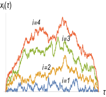
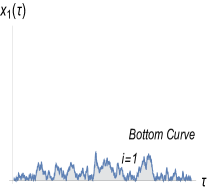
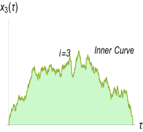
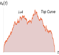
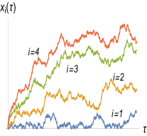
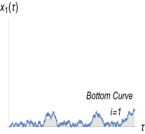
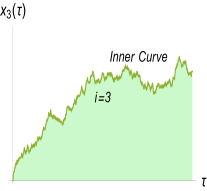
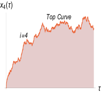
Figure 1: Two instances corresponding to a reunion (top panel) and a meander (bottom panel) of $N$ Vicious paths with reflective boundary conditions at $x=0$, generated by the method explained in the text. We also show the corresponding areas for the bottom, one of the inners, and the top curves.

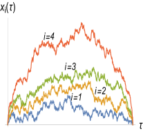
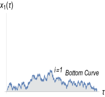
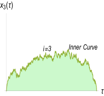
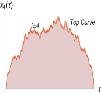
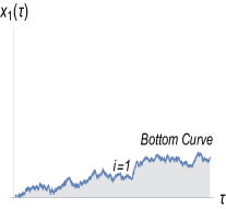
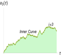
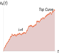
Figure 2: Two instances corresponding to a reunion (top panel) and a meander (bottom panel) of $N$ Vicious paths with absorbing boundary conditions at $x=0$ and generated by the method explained in the text. We also show the corresponding areas for the bottom, one of the inners, and the top curves.

To estimate the different PDFs we have taken $K=10^{3}$ and we have subsequently generated $\mathcal{N}=10^{5}$ $\Xi(t)$ matrices for the four different process. For each instance $s=1,\ldots,\mathcal{N}$ the area swept by each path is estimated as

$$\begin{split}A^{(s)}_{i}=\sum_{k=0}^{K}\lambda^{(s)}_{i}(k)\,,\quad\quad i=1,\ldots,N\,.\end{split}$$ (23)

where $\bm{\lambda}(k)=(-\lambda_{N}(k),\ldots,-\lambda_{1}(k),\lambda_{1}(k),\ldots,\lambda_{N}(k))$ are the eigenvalues of the matrix $\Xi$. This area is then rescaled to the $x$-variable $x^{(s)}_{i}=A^{(s)}_{i}/K^{3/2}$. Finally, the sample set $\{x_{i}^{(s)}\}_{s=1}^{\mathcal{N}}$ for each area $i=1,\ldots,N$, is used to estimate the PDFs as:

$$\begin{split}\mathcal{P}_{N}^{(i)}(x)=\frac{1}{\mathcal{N}}\sum_{s=1}^{\mathcal{N}}\delta\left(x-x_{i}^{(s)}\right)\,\quad\quad i=1,\ldots,N\,.\end{split}$$ (24)

Here we focus on the PDF $Q_{N}(x)$ of the accumulated area. An instance of the four processes can be found in figures 1 and 2.
Results of the PDFs estimated by Monte Carlo simulations and comparison with the theoretical formulas for the PDF $Q_{N}(x)$ of the accumulated area are reported in figure 3 for both types of boundary conditions.

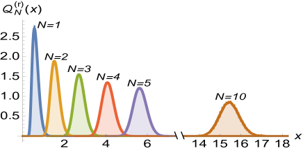
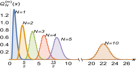
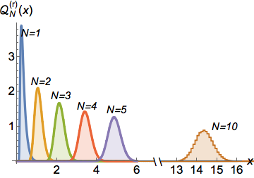
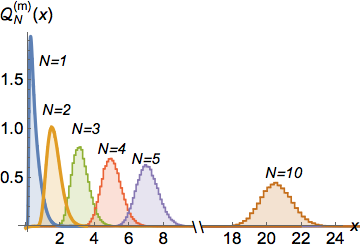
Figure 3: Plots for $\mathcal{Q}^{(r,m)}_{N}(x)$ for $N=1,2,3,4$ and $10$. The top plots corresponds to absorbing boundary conditions, while the bottom plots are for reflecting boundary conditions. Thick solid lines the theoretical results given by (19). All PDFs have been estimated by generating $10^{5}$ samples.

Looking at these figures some points are in order: the comparison between the set of formulas (19) and (21) and Monte Carlo estimates could be done up to $N=10$ and $N=9$, respectively, as otherwise the numerical evaluation of these exact formulas becomes prohibitively long. For the formulas (20) and (22) we have the an additional numerical problem due to the evaluation of the $B_{N}$ and, as a consequence, the comparison with Monte Carlo simulations is performed up to $N=2$ in both cases.

9 Conclusions

In this work we have generalised the Airy distribution function of the area swept by one Brownian particle performing a reunion to the case of the accumulated area swept by $N$ vicious Brownian particles. The exact formulas have been contrasted with Monte Carlo simulations showing perfect agreement.
There are several open problems which we are currently investigating. First of all, whereas obtaining exact expressions for negative moments of the distribution of the accumulated area swept by $N$ vicious walkers is rather simple, we wonder whether it is possible to obtain exacts expressions for the positive moments, perhaps generalising the techniques used for the case of one walker that can be found, for instance, in Takacs1991 ; Takacs1993 ; Kearney2007 . Secondly, we ponder whether it is possible to find exact formulas for the distribution of the area swept by either the bottom or the top paths. Within QMf this entails to being able to construct $N$-particle eigenfunctions for distinguishable fermions. As this seems to be a daunting task, at the very least it would be interesting to study the properties of these distributions numerically. This can be done fairly efficiently, in particular for rate events, by combining the mapping to RMT we have used here together with the Wang-Landau algorithm, a numerical technique that has been used in a similar context to study the statistics of extreme eigenvalues Saito2010 . This analysis can obviously be extended to the cases in which the distribution of jumps of the Brownian motion comes from either thick or thin tails.

Appendix A Taylor expansion of Slater’s determinant

In this secion we discuss the Taylor expansion of a Slater determinant. Starting form the definition of the determinant and doing a Taylor expansion we write:

$$\begin{split}\det_{1\leq i,j\leq N}\varphi_{n_{i}}(z_{j})&=\sum_{P\in S_{N}}\text{sign}(P)\prod_{i=1}^{N}\varphi_{n_{P}(i)}(z_{i})\\ &=\sum_{P\in S_{N}}\text{sign}(P)\sum_{\ell_{1},\ldots,\ell_{N}\geq 0}\frac{z_{1}^{\ell_{1}}\cdots z_{N}^{\ell_{N}}}{\ell_{1}!\cdots\ell_{N}!}\prod_{i=1}^{N}\varphi^{(\ell_{i})}_{n_{P(i)}}(0)\\ &=\sum_{\ell_{1},\ldots,\ell_{N}\geq 0}\frac{z_{1}^{\ell_{1}}\cdots z_{N}^{\ell_{N}}}{\ell_{1}!\cdots\ell_{N}!}\det_{1\leq i,j\leq N}\varphi^{(\ell_{i})}_{n_{j}}(0)\,.\end{split}$$ (25)

Due to the antisymmetric properties of the determinant, only those terms in the multiple sum with different values of $\ell$’s are different from zero. With this in mind we rewrite the sum over the $\bm{\ell}=(\ell_{1},\ldots,\ell_{N})$ as a sum over over $U_{N}$ of ordered indices (let’s say $\ell_{1}<\ell_{2}<\cdots<\ell_{N}$) and then we sum over its permutation, viz.

$$\begin{split}\det_{1\leq i,j\leq N}\varphi_{n_{i}}(z_{j})&=\sum_{\ell_{1},\ldots,\ell_{N}\geq 0}\frac{z_{1}^{\ell_{1}}\cdots z_{N}^{\ell_{N}}}{\ell_{1}!\cdots\ell_{N}!}\det_{1\leq i,j\leq N}\varphi^{(\ell_{i})}_{n_{j}}(0)\\ &=\sum_{\bm{\ell}\in U_{N}}\frac{1}{\ell_{1}!\cdots\ell_{N}!}\sum_{P\in S_{N}}z_{1}^{\ell_{P(1)}}\cdots z_{N}^{\ell_{P(N)}}\det_{1\leq i,j\leq N}\varphi^{(\ell_{P(i)})}_{n_{j}}(0)\\ &=\sum_{\bm{\ell}\in U_{N}}\frac{1}{\ell_{1}!\cdots\ell_{N}!}\sum_{P\in S_{N}}\text{sign}(P)z_{1}^{\ell_{P(1)}}\cdots z_{N}^{\ell_{P(N)}}\det_{1\leq i,j\leq N}\varphi^{(\ell_{i})}_{n_{j}}(0)\\ &=\sum_{\bm{\ell}\in U_{N}}\frac{1}{\ell_{1}!\cdots\ell_{N}!}\det_{1\leq i,j\leq N}[z_{i}^{\ell_{j}}]\det_{1\leq i,j\leq N}[\varphi^{(\ell_{i})}_{n_{j}}(0)]\,,\end{split}$$ (26)

as we wanted to show.

Appendix B Reunion

For the normalisation factor we need to derive the propagator of $N$ vicious walkers in the semi-infinite line. This propagator is this case can be written as follows

$$\begin{split}G_{0}(\bm{y},T|\bm{x},0)=\frac{1}{T^{N/2}}\left(\frac{2}{\pi}\right)^{N}\int_{0}^{\infty}\cdots\int_{0}^{\infty}dq_{1}\cdots dq_{N}\Phi^{(0)}_{\bm{q}}\left(\frac{\bm{y}}{\sqrt{T}}\right)\Phi^{(0)}_{\bm{q}}\left(\frac{\bm{x}}{\sqrt{T}}\right)e^{-\frac{1}{2}\bm{q}^{2}}\,,\end{split}$$ (27)

where $\Phi^{(0)}_{\bm{q}}(\bm{x})=(1/\sqrt{N!})\det_{1\leq i,j\leq N}[\sin(q_{i}x_{j})]$. Using the Taylor expansion formula for the Slater determinant we arrive at

$$\begin{split}\Phi^{(0)}_{\bm{q}}(\bm{x})=\frac{1}{\sqrt{N!}}\sum_{\bm{s}\in U_{N}}\frac{1}{(2s_{1}+1)!\cdots(2s_{N}+1)!}\det_{1\leq i,j\leq N}[x_{i}^{2s_{j}+1}]\det_{1\leq i,j\leq N}[q_{i}^{2s_{j}+1}(-1)^{s_{j}}]\,,\end{split}$$ (28)

with $\bm{s}=(s_{1},\ldots,s_{N})$. Noticing that the lowest contribution is obtained by of $s_{i}=i-1$, we obtain

$$\begin{split}\Phi^{(0)}_{\bm{q}}\left(\frac{\bm{x}}{\sqrt{T}}\right)&\simeq\beta_{N}T^{-\frac{N^{2}}{2}}\left[\prod_{i=1}^{N}x_{i}\right]\Delta_{N}\left(x_{1}^{2},\ldots,x_{N}^{2}\right)\left[\prod_{i=1}^{N}q_{i}\right]\Delta_{N}(q_{1}^{2},\ldots q_{N}^{2})\,,\end{split}$$ (29)

with $\beta_{N}=(-1)^{\frac{N(N-1)}{2}}/[1!\cdots(2N-1)!\sqrt{N!}]$. At this stage we notice that the propagator goes like

$$\begin{split}G_{0}(\bm{\epsilon},T|\bm{x},\epsilon)&\simeq\beta^{2}_{N}T^{-\frac{1}{2}N(2N+1)}\left[\prod_{i=1}^{N}\epsilon^{2}_{i}\right]\Delta^{2}_{N}\left(\epsilon_{1}^{2},\ldots,\epsilon_{N}^{2}\right)B_{N}\,,\\ B_{N}&=\left(\frac{2}{\pi}\right)^{N}\int_{0}^{\infty}\cdots\int_{0}^{\infty}dq_{1}\cdots dq_{N}e^{-\frac{1}{2}\bm{q}^{2}}\left[\prod_{i=1}^{N}q_{i}^{2}\right]\Delta_{N}^{2}(q_{1}^{2},\cdots,q^{2}_{N})\end{split}$$ (30)

where the constant $B_{N}$ is derived in appendix D.
For reflecting boundary conditions the expression for the propagator is the same but with the Slater determinant given by $\Phi^{(0)}_{\bm{q}}(\bm{x})=(1/\sqrt{N!})\det_{1\leq i,j\leq N}[\cos(q_{i}x_{j})]$. Using the expansion formula for the Slater determinant we arrive at

$$\begin{split}\Phi^{(0)}_{\bm{q}}(\bm{x}/\sqrt{T})=\frac{1}{\sqrt{N!}}\sum_{\bm{s}\in U_{N}}\frac{1}{(2s_{1})!\cdots(2s_{N})!}\det_{1\leq i,j\leq N}[T^{-s_{j}}x_{i}^{2s_{j}}]\det_{1\leq i,j\leq N}[q_{i}^{2s_{j}}(-1)^{s_{j}}]\,,\end{split}$$ (31)

with $\bm{s}=(s_{1},\ldots,s_{N})$. Noticing that the lowest contribution is obtained by of $s_{i}=i-1$, we obtain

$$\begin{split}\Phi^{(0)}_{\bm{q}}\left(\frac{\bm{x}}{\sqrt{T}}\right)&\simeq\beta_{N}T^{-\frac{N(N-1)}{2}}\Delta_{N}\left(x_{1}^{2},\ldots,x_{N}^{2}\right)\left[\prod_{i=1}^{N}q_{i}\right]\Delta_{N}(q_{1}^{2},\ldots q_{N}^{2})\,,\end{split}$$ (32)

with $\beta_{N}=(-1)^{\frac{N(N-1)}{2}}/[0!\cdots(2(N-1))!\sqrt{N!}]$. At this stage we notice that the propagator goes like

$$\begin{split}G_{0}(\bm{\epsilon},T|\bm{x},\epsilon)&\simeq\beta^{2}_{N}T^{-\frac{N(2N-1)}{2}}\Delta^{2}_{N}\left(\epsilon_{1}^{2},\ldots,\epsilon_{N}^{2}\right)F_{N}\,,\\ F_{N}&=\left(\frac{2}{\pi}\right)^{N}\int_{0}^{\infty}\cdots\int_{0}^{\infty}dq_{1}\cdots dq_{N}e^{-\frac{1}{2}\bm{q}^{2}}\Delta_{N}^{2}(q_{1}^{2},\cdots,q^{2}_{N})\end{split}$$ (33)

where the constant $F_{N}$ is derived in appendix D.

Appendix C Meander

For the case of a meander of $N$ vicious walkers (a star with a wall) we need to integrate over the final position $\bm{x}$. Using the Taylor expansion of the Slater determinant as explained in the main text we can write

$$\begin{split}\int_{\bm{W}_{N}}d^{N}\bm{x}G_{N}^{(1)}(\bm{x},T|\bm{\epsilon},0)&=\sum_{\bm{n}}\int_{\bm{W}_{N}}d^{N}\bm{x}\,\Phi^{(1)}_{\bm{n}}(\bm{x})\overline{\Phi}^{(1)}_{\bm{n}}(\bm{\epsilon})e^{-E^{(1)}_{\bm{n}}T}\\ &\simeq(2\lambda)^{\frac{N^{2}}{3}}\gamma_{N}\left[\prod_{i=1}^{N}\epsilon_{i}\right]\Delta_{N}(\epsilon_{1}^{2},\ldots\epsilon_{N}^{2})\,\sum_{\bm{n}}B_{N}(\alpha_{n_{1}},\ldots,\alpha_{n_{N}})\Delta_{N}(\alpha_{n_{1}},\dots\alpha_{n_{N}})e^{-E^{(1)}_{\bm{n}}T}\,,\end{split}$$ (34)

where we have defined

$$\begin{split}B_{N}(\alpha_{n_{1}},\ldots,\alpha_{n_{N}})&=\frac{1}{\prod_{i=1}^{N}\text{Ai}^{\prime}(-\alpha_{n_{i}})}\int_{\bm{W}_{N}}d^{N}\bm{x}\det_{1\leq i,j\leq N}\left[\text{Ai}(x_{j}-\alpha_{n_{i}})\right]\,.\end{split}$$ (35)

Similarly, the propagator in the denominator goes like

$$\begin{split}\int_{\bm{W}_{N}}d^{N}\bm{x}G_{N}^{(0)}(\bm{x},T|\bm{\epsilon},0)&\simeq T^{-\frac{N^{2}}{2}}\gamma_{N}F_{N}\left[\prod_{i=1}^{N}\epsilon_{i}\right]\Delta_{N}(\epsilon_{1}^{2},\ldots\epsilon_{N}^{2})\end{split}$$ (36)

where $F_{N}$ is a constant with no simple expression.
For reflecting boundary conditions we have instead the following expression for the numerator

$$\begin{split}&\int_{\bm{W}_{N}}d^{N}\bm{x}G_{N}^{(1)}(\bm{x},T|\bm{\epsilon},0)=\sum_{\bm{n}}\int_{\bm{W}_{N}}d^{N}\bm{x}\Psi_{\bm{n}}^{(1)}(\bm{x})\overline{\Psi}_{\bm{n}}^{(1)}(\bm{\epsilon})e^{-E_{\bm{n}}^{(1)}T}\\ &=\frac{\delta_{N}}{N!}\Delta_{N}(x_{1}^{2},\ldots,x_{N}^{2})\sum_{\bm{n}}\frac{\Delta_{N}(\beta_{n_{1}},\ldots,\beta_{n_{N}})}{\beta_{n_{1}}\cdots\beta_{n_{N}}}e^{-E_{\bm{n}}^{(1)}T}(2\lambda)^{\frac{N(2N-1)}{6}}(2\lambda)^{N/6}\\ &\int_{\bm{W}_{N}}d^{N}\bm{x}\frac{1}{\prod_{i=1}^{N}\text{Ai}(-\beta_{n_{i}})}\det_{1\leq i,j\leq N}[\text{Ai}((2\lambda)^{1/3}x_{j}-\beta_{n_{i}})]\\ &=\frac{\delta_{N}}{N!}\Delta_{N}(x_{1}^{2},\ldots,x_{N}^{2})(2\lambda)^{\frac{N(2N-1)}{6}-N/6}\sum_{\bm{n}}\frac{\Delta_{N}(\beta_{n_{1}},\ldots,\beta_{n_{N}})}{\beta_{n_{1}}\cdots\beta_{n_{N}}}e^{-E_{\bm{n}}^{(1)}T}\\ &\int_{\bm{W}_{N}}d^{N}\bm{z}\frac{1}{\prod_{i=1}^{N}\text{Ai}(-\beta_{n_{i}})}\det_{1\leq i,j\leq N}[\text{Ai}(z_{j}-\beta_{n_{i}})]\\ &=\frac{\delta_{N}}{N!}\Delta_{N}(x_{1}^{2},\ldots,x_{N}^{2})(2\lambda)^{\frac{N(N-1)}{3}}\sum_{\bm{n}}\frac{\Delta_{N}(\beta_{n_{1}},\ldots,\beta_{n_{N}})}{\beta_{n_{1}}\cdots\beta_{n_{N}}}e^{-E_{\bm{n}}^{(1)}T}\\ &\frac{1}{\prod_{i=1}^{N}\text{Ai}(-\beta_{n_{i}})}\int_{\bm{W}_{N}}d^{N}\bm{z}\det_{1\leq i,j\leq N}[\text{Ai}(z_{j}-\beta_{n_{i}})]\end{split}$$ (37)

Appendix D On the normalisation constants

Here we derive the expressions for the two normalisation constants for the case of reunions for absorbing and reflecting boundary conditions. For both cases we recall the well-known result of Selberg’s integral forrester2010log :

$$\begin{split}\frac{1}{N!}\int_{0}^{\infty}\cdots\int_{0}^{\infty}|\Delta(x_{1},\ldots,x_{N})|^{2c}\prod_{i=1}^{N}x_{i}^{a-1}e^{-x_{i}}dx_{i}=\prod_{j=0}^{N-1}\frac{\Gamma(a+jc)\Gamma((j+1)c)}{\Gamma(c)}\end{split}$$ (38)

For the constant $B_{N}$ we do the change of variables $q_{i}^{2}/2=y_{i}$ so that $q_{i}dq_{i}=dy_{i}$ or $dq_{i}=\frac{dy_{i}}{\sqrt{2y_{i}}}$, so we can write

$$\begin{split}B_{N}&=\left(\frac{2}{\pi}\right)^{N}\int_{0}^{\infty}\cdots\int_{0}^{\infty}dq_{1}\cdots dq_{N}e^{-\frac{1}{2}\bm{q}^{2}}\left[\prod_{i=1}^{N}q_{i}^{2}\right]\Delta_{N}^{2}(q_{1}^{2},\cdots,q^{2}_{N})\\ &=\left(\frac{2}{\pi}\right)^{N}2^{-N/2}2^{N}2^{N(N-1)}\int_{0}^{\infty}\cdots\int_{0}^{\infty}dy_{1}\cdots dy_{N}\prod_{i=1}^{N}e^{-y_{i}}y_{i}^{-1/2}\left[\prod_{i=1}^{N}y_{i}\right]\Delta_{N}^{2}(y_{1},\cdots,y_{N})\\ &=\frac{2^{\frac{1}{2}N(2N+1)}}{\pi^{N}}N!\prod_{j=0}^{N-1}\Gamma\left(\frac{3}{2}+j\right)\Gamma(j+1)=\frac{2^{\frac{1}{2}N(2N+1)}}{\pi^{N}}\prod_{j=0}^{N-1}\Gamma(2+j)\Gamma\left(\frac{3}{2}+j\right)\end{split}$$ (39)

Similarly for the case of reflecting boundary conditions we have

$$\begin{split}F_{N}&=\left(\frac{2}{\pi}\right)^{N}\frac{1}{2^{N/2}}2^{N(N-1)}\int_{0}^{\infty}\cdots\int_{0}^{\infty}dy_{1}\cdots dy_{N}\Delta_{N}^{2}(y_{1},\cdots,y_{N})\prod_{i=1}^{N}y_{i}^{-1/2}e^{-y_{i}}\\ &=N!\frac{2^{\frac{N(2N-1)}{2}}}{\pi^{N}}\prod_{j=0}^{N-1}\Gamma\left(\frac{1}{2}+j\right)\Gamma\left(j+1\right)=\frac{2^{\frac{N(2N-1)}{2}}}{\pi^{N}}\prod_{j=0}^{N-1}\Gamma\left(\frac{1}{2}+j\right)\Gamma\left(j+2\right)\end{split}$$ (40)

Appendix E Derivatives of $F(x,\gamma)$

Starting from the following expression for $F(x,\gamma)$:

$$\begin{split}F(x,\gamma)=\frac{\sqrt{3}}{x\sqrt{\pi}}u^{2/3}(x,\gamma)e^{-u(x,\gamma)}U\left(\frac{1}{6},\frac{4}{3},u(x,\gamma)\right)\,,\quad u(x,\gamma)=\frac{2\gamma^{3}}{27x^{2}}\,,\end{split}$$ (41)

and using the following property

$$\begin{split}x\frac{\partial U(a,b,x)}{\partial x}=(a-b+x)U(a,b,x)-U(a-1,b,x)\,,\end{split}$$ (42)

we notice that we can write the expression

$$\begin{split}\frac{\partial^{n}F(x,\gamma)}{\partial x^{n}}=\frac{\sqrt{3}}{x^{n+1}\sqrt{\pi}}u^{2/3}(x,\gamma)e^{-u(x,\gamma)}\sum_{\ell=0}^{n}C^{(n)}_{\ell}U\left(\frac{1}{6}-\ell,\frac{4}{3},u(x,\gamma)\right)\,.\end{split}$$ (43)

for some set of coefficients $\{C^{(n)}_{\ell}\}$ still to be determined. The expression (43) is certainly correct for $n=1$ and $n=2$. Let us them assume is holds for any $n$ and performe one more derivative with respect to $n$:

$$\begin{split}\frac{\partial^{n+1}F(x,\gamma)}{\partial x^{n+1}}&=\frac{1}{x^{n+2}\sqrt{3\pi}}u^{2/3}(x,\gamma)e^{-u(x,\gamma)}\\ &\sum_{\ell=0}^{n}C^{(n)}_{\ell}\left[(-7-3n+6u(x,\gamma))U\left(\frac{1}{6}-\ell,\frac{4}{3},u(x,\gamma)\right)-6u(x,\gamma)U^{\prime}\left(\frac{1}{6}-\ell,\frac{4}{3},u(x,\gamma)\right)\right]\,.\end{split}$$ (44)

But using the property (42), we can write

$$\begin{split}u(x,\gamma)U^{\prime}\left(\frac{1}{6}-\ell,\frac{4}{3},u(x,\gamma)\right)=\left(\frac{1}{6}-\ell-\frac{4}{3}+u\right)U\left(\frac{1}{6}-\ell,\frac{4}{3},u(x,\gamma)\right)-U\left(\frac{1}{6}-\ell-1,\frac{4}{3},u(x,\gamma)\right)\,.\end{split}$$ (45)

Gathering results we find

$$\begin{split}\frac{\partial^{n+1}F(x,\gamma)}{\partial x^{n+1}}&=\frac{\sqrt{3}}{x^{n+2}\sqrt{\pi}}u^{2/3}(x,\gamma)e^{-u(x,\gamma)}\\ &\sum_{\ell=0}^{n}C^{(n)}_{\ell}\left[(-n+2\ell)U\left(\frac{1}{6}-\ell,\frac{4}{3},u(x,\gamma)\right)+2U\left(\frac{1}{6}-\ell-1,\frac{4}{3},u(x,\gamma)\right)\right]\,.\end{split}$$ (46)

On the other hand, we want to write this result as (43) for $n\to n+1$. This implies to rewrite the sum as:

$$\begin{split}&\sum_{\ell=0}^{n}C^{(n)}_{\ell}\left[(-n+2\ell)U\left(\frac{1}{6}-\ell,\frac{4}{3},u(x,\gamma)\right)+2U\left(\frac{1}{6}-\ell-1,\frac{4}{3},u(x,\gamma)\right)\right]\\ &=\sum_{\ell=0}^{n}C^{(n)}_{\ell}(-n+2\ell)U\left(\frac{1}{6}-\ell,\frac{4}{3},u(x,\gamma)\right)+2\sum_{\ell=0}^{k}C^{(n)}_{\ell}U\left(\frac{1}{6}-\ell-1,\frac{4}{3},u(x,\gamma)\right)\\ &=\sum_{\ell=0}^{n}C^{(n)}_{\ell}(-n+2\ell)U\left(\frac{1}{6}-\ell,\frac{4}{3},u(x,\gamma)\right)+2\sum_{\ell=1}^{n+1}C^{(n)}_{\ell-1}U\left(\frac{1}{6}-\ell,\frac{4}{3},u(x,\gamma)\right)\\ &=\sum_{\ell=0}^{n+1}C^{(n+1)}_{\ell}U\left(\frac{1}{6}-\ell,\frac{4}{3},u(x,\gamma)\right)\,.\end{split}$$ (47)

This results in the following set of recurrence relations for the set of coefficents $\{C_{\ell}^{(n)}\}$:

$$\begin{split}C^{(n+1)}_{0}&=-nC_{0}^{(n)}\,,\\ C_{\ell}^{(n+1)}&=C_{\ell}^{(n)}(-n+2\ell)+2C_{\ell-1}^{(n)}\,,\quad\ell=1,\ldots,n\,,\\ C_{n+1}^{(n+1)}&=2C_{n}^{(n)}\,,\end{split}$$ (48)

with the initial condition $C_{0}^{(0)}=1$. By checking explicitly the value of some of these coeffcients, and with the help of the Sloane database, we arrive at the solution:

$$\begin{split}C^{(n)}_{\ell}=\frac{n!}{2^{n-2\ell}(n-\ell)!(2\ell-n)!}\,,\quad\ell=0,\ldots,n\,.\end{split}$$ (49)

A Similar analysis can be perform ny doing derivatives with respect to $\gamma$. Starting from (43) one notices that

$$\begin{split}\frac{\partial^{k+n}F(x,\gamma)}{\partial\gamma^{k}\partial x^{n}}=\frac{\sqrt{3}}{x^{n+1}\sqrt{\pi}\gamma^{k}}u^{2/3}(x,\gamma)e^{-u(x,\gamma)}\sum_{\ell=0}^{n}\sum_{s=0}^{k}C^{(n)}_{\ell}D^{(k)}_{s}(\ell)U\left(\frac{1}{6}-\ell-s,\frac{4}{3},u(x,\gamma)\right)\,,\end{split}$$ (50)

for some set of coefficients $\{D_{s}^{(k)}(\ell)\}$. Performing one more derivative with respect to $\gamma$ allows us to arrive at the following set of recurrence relations for those, viz.

$$\begin{split}D_{0}^{(k+1)}(\ell)&=-\left(\frac{3}{2}+k+3\ell\right)D_{0}^{(k)}(\ell)\,,\\ D_{s}^{(k+1)}(\ell)&=-\left(\frac{3}{2}+k+3\ell+3s\right)D_{s}^{(k)}(\ell)-3D_{s-1}^{(k)}(\ell)\,,\quad\quad s=1,\ldots,k\,,\\ D_{k+1}^{(k+1)}(\ell)&=-3D_{k}^{(k)}(\ell)\,,\end{split}$$ (51)

with the initial condition $D_{0}^{(0)}(\ell)=1$. As we are only interested in the orders $k=0$ and $k=2$, we do not need a general solution. This yields

$$\begin{split}D_{0}^{(0)}(\ell)&=1\,,\\ D_{0}^{(1)}(\ell)&=-\frac{3}{2}\left(1+2\ell\right)\,,\quad\quad D_{1}^{(1)}(\ell)=-3\,\\ D_{0}^{(2)}(\ell)&=\frac{3}{4}(1+2\ell)(5+6\ell)\,,\quad\quad D_{1}^{(2)}(\ell)=3(7+6\ell)\,,\quad\quad D_{2}^{(2)}(\ell)=9\,.\end{split}$$ (52)

Appendix F Moments

We first recall the following identity

$$\begin{split}\int_{0}^{\infty}dss^{\mu}e^{-xs}=\frac{\Gamma(\mu+1)}{x^{1+\mu}}\,.\end{split}$$ (53)

From here we write

$$\begin{split}M_{-(1+\mu)}&=\int_{0}^{\infty}dxx^{-(1+\mu)}F(x)\\ &=\frac{1}{\Gamma(\mu+1)}\int_{0}^{\infty}dxF(x)\int_{0}^{\infty}dss^{\mu}e^{-xs}\\ &=\frac{1}{\Gamma(\mu+1)}\int_{0}^{\infty}dss^{\mu}\int_{0}^{\infty}dxF(x)e^{-xs}\\ &=\frac{1}{\Gamma(\mu+1)}\int_{0}^{\infty}dss^{\mu}\widehat{F}(s)\\ &=\frac{1}{\Gamma(\mu+1)}\int_{0}^{\infty}dss^{\mu+E}e^{-as^{2/3}}\end{split}$$ (54)

But

$$\begin{split}\int_{0}^{\infty}dss^{\mu+E}e^{-as^{2/3}}&=\int_{0}^{\infty}ds(s^{2/3})^{\frac{3}{2}(\mu+E)}e^{-as^{2/3}}\\ &=\frac{3}{2}\int_{0}^{\infty}dyy^{\frac{3}{2}(\mu+E)+1/2}e^{-ay}\\ &=\frac{3}{2}a^{-\frac{3}{2}(\mu+E+1)}\int_{0}^{\infty}dyy^{\frac{3}{2}(\mu+E)+1/2}e^{-y}\\ &=\frac{3}{2}a^{-\frac{3}{2}(\mu+E+1)}\Gamma\left(\frac{3}{2}(\mu+E+1)\right)\end{split}$$ (55)

Thus denoting $\nu=1+\mu$ we finally have

$$\begin{split}M_{-\nu}=\frac{3}{2}a^{-\frac{3}{2}(\nu+E)}\frac{\Gamma\left(\frac{3}{2}(\nu+E)\right)}{\Gamma(\nu)}\end{split}$$ (56)

References

- (1) Adler, M., van Moerbeke, P., Vanderstichelen, D.: Non-intersecting brownian motions leaving from and going to several points. Physica D 241(5), 443 – 460 (2012)
- (2) Baik, J.: Random vicious walks and random matrices. Commun. Pure Appl. Math. 53(11), 1385–1410 (2000)
- (3) Barkai, E., Aghion, E., Kessler, D.: From the area under the bessel excursion to anomalous diffusion of cold atoms. Physical Review X 4, 021,036 (2014)
- (4) Bleher, P., Delvaux, S., Kuijlaars, A.B.J.: Random matrix model with external source and a constrained vector equilibrium problem. Commun. Pure Appl. Math. 64(1), 116–160 (2011)
- (5) Borodin, A., Kuan, J.: Random surface growth with a wall and plancherel measures for . Commun. Pure Appl. Math. 63(7), 831–894 (2010)
- (6) Daems, E., Kuijlaars, A.: Multiple orthogonal polynomials of mixed type and non-intersecting brownian motions. J Appr. Th. 146(1), 91 – 114 (2007)
- (7) Darling, D.A.: On the supremum of a certain gaussian process. The Annals of Probability 11, 803 (1983)
- (8) Ferrari, P.L., Praehofer, M.: One-dimensional stochastic growth and Gaussian ensembles of random matrices. ArXiv (2005)
- (9) Forrester, P.J.: Random walks and random permutations. J. Phys. A 34(31), L417 (2001)
- (10) Forrester, P.J.: Log-gases and random matrices (LMS-34). Princeton University Press (2010)
- (11) Forrester, P.J., Majumdar, S.N., Schehr, G.: Non-intersecting brownian walkers and yang–mills theory on the sphere. Nucl. Phys. B 844(3), 500–526 (2011)
- (12) Johansson, K.: Discrete polynuclear growth and determinantal processes. Comm. Math. Phys. 242(1-2), 277–329 (2003)
- (13) Katori, M., Tanemura, H.: Symmetry of matrix-valued stochastic processes and noncolliding diffusion particle systems. J. Math Phys. 45, 3058 (2004)
- (14) Kearney, M.J., Majumdar, S.N., Martin, R.J.: The first-passage area for drifted brownian motion and the moments of the airy distribution. J. Phys A 40, F863 (2007)
- (15) Kessler, D., Medallion, S., Barkai, E.: The distribution of the area under a bessel excursion and its moments. Journal of Statistical Physics 156, 686–706 (2014)
- (16) Kobayashi, N., Izumi, M., Katori, M.: Maximum distributions of bridges of noncolliding brownian paths. Phys. Rev. E 78, 051,102 (2008)
- (17) Laurenzi: Polynomials associated with the higher derivatives of the airy functions and . arXiv:1110.2025 (2011)
- (18) Louchard, G.: Kac’s formula, levy’s local time and brownian excursion. J. Appl. Prob 21, 479 (1984)
- (19) Majumdar, S., Comtet, A.: Exact maximal height distribution of fluctuating interfaces. Phys. Rev. Lett. 92, 225,501 (2004)
- (20) Majumdar, S.N., Comtet, A.: Airy distribution function: from the area under a brownian excursion to the maximal height of fluctuating interfaces. J. Stat. Phys 119, 777–826 (2005)
- (21) Medalion, S., Aghion, E., Meirovitch, H., Barkai, E., Kessler, D.A.: Fluctuations of ring polymers. arXiv:1501.06143 (2015)
- (22) Nadal, C., Majumdar, S.N.: Nonintersecting brownian interfaces and wishart random matrices. Phys. Rev. E 79, 061,117 (2009)
- (23) Nagao, T.: Dynamical correlations for vicious random walk with a wall. Nucl. Phys. B 658(3), 373 – 396 (2003)
- (24) Novak, J.: Vicious walkers and random contraction matrices. Int. Math. Res. Notices 17, 3310–3327 (2009)
- (25) N.Saito, Yukito, I., Hukushima, K.: Multicanonical sampling of rare events in random matrices. Phys Rev E 82, 031,142 (2010)
- (26) Rambeau, J., Schehr, G.: Extremal statistics of curved growing interfaces in 1+1 dimensions. Eur. Lett. 91(6), 60,006 (2010)
- (27) Schehr, G., Majumdar, S.N., Comtet, A., Forrester, P.J.: Reunion probability of n vicious walkers: typical and large fluctuations for large n. J. Stat. Phys. pp. 1–40 (2013)
- (28) Schehr, G., Majumdar, S.N., Comtet, A., Randon-Furling, J.: Exact distribution of the maximal height of vicious walkers. Phys. Rev. Lett. 101, 150,601 (2008)
- (29) Takács, L.: A bernoulli excursion and its various applications. Ad. in App. Prob. 23, 557 (1991)
- (30) Takács, L.: On the distribution of the integral of the absolute value of the brownian motion. Ann. of App. Prob. 3, 186 (1993)
- (31) Takacs, L.: Limit distributions for the bernoulli meander. J. Appl. Prob. 32, 375 (1995)
- (32) Tracy, C.A., Widom, H.: Nonintersecting brownian excursions. Ann. Appl. Probab. 17, 953–979 (2007)