Time-dependent toroidal compactification proposals and the Bianchi type II model: classical and quantum solutions

Abstract

In this work we construct an effective four-dimensional model by compactifying a ten-dimensional theory of gravity coupled with a real scalar dilaton field on a time-dependent torus without the contributions of fluxes as first approximation. This approach is applied to anisotropic cosmological Bianchi type II model for which we study the classical coupling of the anisotropic scale factors with the two real scalar moduli produced by the compactification process. Also, we present some solutions to the corresponding Wheeler-DeWitt (WDW) equation in the context of Standard Quantum Cosmology and we claim that these quantum solution are generic in the moduli scalar field for all Bianchi Class A models. Also we gives the relation to these solutions for asymptotic behavior to large argument in the corresponding quantum solution in the gravitational variables and is compared with the Bohm’s solutions, finding that this corresponds to lowest-order WKB approximation.

I Introduction

In the last years there have been several attempts to understand the diverse aspects of cosmology, as the presence of stable vacua and inflationary conditions, in the framework of supergravity and string theory Damour0 ; Horne ; Banks ; Damour1 ; Banks1 ; Kallosh0 ; Kallosh1 ; Baumann . One of the most interesting features emerging from these type of models consists on the study of the consequences of higher dimensional degrees of freedom on the cosmology derived from four-dimensional effective theories Khoury .

Furthermore, it has been pointed out that the presence of extra dimensions leads to an interesting connection with the ekpyrotic model Khoury , which generated considerable activity Kallosh0 ; Kallosh1 ; Enqvist . The essential ingredient in these models (see for instance Khoury ) is to consider an effective action with a graviton and a massless scalar field, the dilaton, describing the evolution of the Universe, while incorporating some of the ideas of pre-big-bang proposal Veneziano in that the evolution of the Universe began in the far past.

On the other hand, it is well known that relativistic theories of gravity such as general relativity or string theories are invariant under reparametrization of time. The quantization of such theories presents a number of problems of principle known as “the problem of time” Isham ; Kuchar . This problem is present in all systems whose classical version is invariant under time reparametrization, leading to its absence at the quantum level. Therefore, the formal question involves how to handle the classical Hamiltonian constraint, $\mathcal{H}\approx 0$, in the quantum theory. Also, connected with the problem of time is the “Hilbert space problem” Isham ; Kuchar referring to the not at all obvious selection of the inner product of states in quantum gravity, and whether there is a need for such a structure at all.

The above features, as it is well known, point out the necessity to construct a consistent theory of gravity at quantum level. One promising attempt is string theory where the structure of the internal space plays a relevant role in the construction of interesting effective models containing cosmological features as the presence of positive valued minima of the scalar potential and slow-roll inflationary conditions. The usual procedure for that is to consider compactification on generalized manifolds, on which internal fluxes have back-reacted, altering the smooth Calabi-Yau geometry and stabilizing all the moduli Baumann .

In the present work we shall consider an alternative procedure about the role played by the moduli. In particular we shall not consider the presence of fluxes, as in string theory, in order to obtain a moduli-dependent scalar potential in the effective theory. Rather, we are going to promote some of the moduli to time-dependent fields by considering the particular case of a ten-dimensional gravity coupled to a time-dependent dilaton compactified on a 6-dimensional torus with a time-dependent Kähler modulus. With the propose to track down the role play by such fields, we are going to ignore the dynamics of the complex structure field (for instance, by assuming that it is already stabilized by the presence of a string field in higher scales).

The work is organized in the following form. In section II we present the construction of our effective action by compactification on a time-dependent torus, while in Section III we study its Lagrangian and Hamiltonian descriptions using as toy model the Bianchi type II cosmological model and we present the general structure for all Bianchi Class A models. Section IV is devoted on finding the corresponding classical solutions for few different cases involving the presence or absence of matter content. In Section V we present some solutions to the corresponding Wheeler-DeWitt (WDW) equation in the context of Standard Quantum Cosmology, resulting the modified Bessel function $\rm(K_{\mu}(z),I_{\mu}(z))$, solutions that in some sense are similar to this find in previous work soc2 . In order that the unnormalized probability density $|\Theta(\Omega,\beta_{\pm})|^{2}$ does not diverge for $\rm|\beta_{\pm}|\to\infty$ and at fixed $\Omega$, which are the gravitational variables, we drop the function $\rm I_{\mu}(z)$, remaining only the function $\rm K_{\mu}(z)$. Also in this section we make an analysis for particular case in the constants in the solution found in the asymptotic behavior for large argument in the gravitational variables and it is compare with the Bohm’s solutions obtained, finding that this corresponds to lowest-order WKB approximation. The Bohm’s solutions was obtained in other decomposition of the quantum WDW equation, related with the Bohm’s formalism, which was applied in the supersymmetric quantum cosmology osb . Finally our conclusions are presented in Section VI.

II Effective model

We start from a ten-dimensional action coupled with a dilaton (which is the bosonic component common to all superstring theories), which after dimensional reduction can be interpreted as a Brans-Dicke like theory Brans . In the string frame, the effective action depends on two time-dependent scalar fields: the dilation $\Phi(t)$ and the Kähler modulus $\sigma(t)$, where the initial high-dimensional (effective) theory is given by

$$S=\frac{1}{2\kappa^{2}_{10}}\int d^{10}X\sqrt{-\hat{G}}\,e^{-2\Phi}\,\Bigg{[}\hat{\mathcal{R}}^{(10)}[\hat{G}_{MN}]+4\,\hat{G}^{MN}\nabla_{M}\,\Phi\,\nabla_{N}\,\Phi\Bigg{]},$$ (1)

with a metric described by

$$ds^{2}=\hat{G}_{MN}\,dX^{M}\,dX^{N}=g_{\mu\nu}\,dx^{\mu}\,dx^{\nu}+h_{mn}\,dy^{m}\,dy^{n},$$ (2)

where $M,N,P,\ldots$ are the indices of the 10-dimensional space, and greek and latin indices correspond to the external and internal space, respectively. The internal metric is given by

$$h_{mn}=e^{-2\sigma(t)}\delta_{mn}.$$ (3)

In order to rewrite it in the Einstein frame, we take as usual, the conformal transformation of the four dimensional metric $g_{\mu\nu}$ as

$$g_{\mu\nu}=e^{2\phi(t)}g^{E}_{\mu\nu},$$ (4)

where $g_{\mu\nu}$ is the metric in the string frame and $g^{E}_{\mu\nu}$ is the metric in Einstein frame and the dilaton has been redefined accordingly as $\phi=\Phi-\frac{1}{2}\,\ln(Vol(X_{6}))$. Notice that in this way, the effective dilaton $\phi$ is also a time-dependent field. Following this notion, we have that the action (1) reads

$$S=\frac{1}{2\kappa^{2}_{4}}\int d^{4}x\sqrt{-g}\bigg{(}\mathcal{R}-6g^{\mu\nu}\nabla_{\mu}\nabla_{\nu}\phi-6g^{\mu\nu}\nabla_{\mu}\nabla_{\nu}{\sigma}-2g^{\mu\nu}\nabla_{\mu}\phi\nabla_{\nu}\phi-96g^{\mu\nu}\nabla_{\mu}\sigma\nabla_{\nu}{\sigma}-36g^{\mu\nu}\nabla_{\mu}\phi\nabla_{\nu}\sigma\bigg{)},$$ (5)

where we have omitted the upper script $E$ in the metric. Now with the expression (5) we proceed to build the Lagrangian and the Hamiltonian of the theory at the classical regimen employing the anisotropic cosmological Bianchi type II model.

III The classical Hamiltonian

In the last section we have built the reduced effective action, now we will construct the classical Hamiltonian from the expression (5). We are going to assume that the background of the extended space (four dimensional) is a Bianchi type II anisotropic cosmological model. In order to do it, let us recall here the canonical formulation in the ADM formalism of the diagonal Bianchi Class A cosmological models. The metric has the form

$$ds^{2}=-N(t)dt^{2}+e^{2\Omega(t)}\,(e^{2\beta(t)})_{ij}\,\omega^{i}\,\omega^{j},$$ (6)

where $N(t)$ is the lapse function, $\beta_{ij}(t)$ is a $3\times 3$ diagonal matrix, $\beta_{ij}=\text{diag}(\beta_{+}+\sqrt{3}\beta_{-},\beta_{+}-\sqrt{3}\beta_{-},-2\beta_{+})$, $\Omega(t)$ and $\beta_{\pm}$ are scalar functions known as Misner variables, $\omega^{i}$ are one-forms that characterize each cosmological Bianchi type model Ryan , and obey the form $d\omega^{i}=\frac{1}{2}C^{i}_{jk}\omega^{j}\wedge\omega^{k}$, with $C^{i}_{jk}$ the structure constants of the corresponding model. The one-forms for the Bianchi type II model are $\omega^{1}=dx^{2}-x^{1}dx^{3}$, $\omega^{2}=dx^{3}$, $\omega^{3}=dx^{1}$. So, the corresponding metric of the Bianchi type II in Misner’s parametrization has the form

$$ds^{2}= -N^{2}dt^{2}+e^{2\Omega-4\beta_{+}}\,\left(dx^{1}\right)^{2}+e^{2\Omega+2\beta_{+}+2\sqrt{3}\beta_{-}}\,\left(dx^{2}\right)^{2}+\left(\left(x^{1}\right)^{2}e^{2\Omega+2\beta_{+}+2\sqrt{3}\beta_{-}}+e^{2\Omega+2\beta_{+}-2\sqrt{3}\beta_{-}}\right)\,\left(dx^{3}\right)^{2}$$

$$-2x^{1}e^{2\Omega+2\beta_{+}+2\sqrt{3}\beta_{-}}\,dx^{2}dx^{3}.$$

substituting $x^{1}=x$, $x^{2}=y$, $x^{3}=z$, we have the following form

$$ds^{2}= -N^{2}dt^{2}+e^{2\Omega-4\beta_{+}}\,dx^{2}+e^{2\Omega+2\beta_{+}+2\sqrt{3}\beta_{-}}\,dy^{2}+\left(x^{2}\,e^{2\Omega+2\beta_{+}+2\sqrt{3}\beta_{-}}+e^{2\Omega+2\beta_{+}-2\sqrt{3}\beta_{-}}\right)\,dz^{2}$$ (7)

$$-2x\,e^{2\Omega+2\beta_{+}+2\sqrt{3}\beta_{-}}\,dy\,dz.$$

The Lagrangian density as effective theory for this model, including an intuitive way the matter content for a barotropic perfect fluid as a first approximation, has the structure Socorro ; Mathur ; odin1 ; odin2

$$\mathcal{L}_{mat}=16\pi G_{N}\sqrt{-g}\rho=16N\pi G_{N}C_{\gamma}e^{-3(1+\gamma)\Omega}$$

where $\gamma$ is the parameter that characterize the epochs in the evolution to the Universe. The Lagrangian that describes this model is given by

$$\mathcal{L}_{II}=\frac{e^{3\Omega}}{N}\left[6\,\dot{\Omega}^{2}-6\,\dot{\beta}^{2}_{+}-6\,\dot{\beta}^{2}_{-}+96\,\dot{\sigma}^{2}+36\,\dot{\phi}\,\dot{\sigma}+2\,\dot{\phi}^{2}+16\,\pi\,G\,N^{2}\,\rho+\frac{1}{2}N^{2}e^{-2\Omega+4\beta_{+}+4\sqrt{3}\beta_{-}}\right].$$ (8)

Computing the momenta associated to the moduli fields $(\phi,\sigma)$ and Misner variables $(\Omega,\beta_{+},\beta_{-})$ and using the Legendre transformation we obtain the Hamiltonian density for this model

$$\mathcal{H}_{II}=\frac{e^{-3\Omega}}{24}\left[\Pi_{\Omega}^{2}-\Pi_{+}^{2}-\Pi_{-}^{2}-\frac{48}{11}\Pi_{\phi}^{2}+\frac{18}{11}\Pi_{\phi}\,\Pi_{\sigma}-\frac{1}{11}\Pi_{\sigma}^{2}-384\,\pi\,G_{N}\,C_{\gamma}\,e^{3(1-\gamma)\Omega}-12\,e^{4(\Omega+\beta_{+}+\sqrt{3}\beta_{-})}\right].$$ (9)

We can introduce a new set of variables that involving the Misner variables $(\Omega,\beta_{+},\beta_{-})$ in the gravitational part ,

$$\beta_{1} =\Omega+\beta_{+}+\sqrt{3}\beta_{-}, \qquad\Omega =\frac{1}{3}\left(\beta_{1}+\beta_{2}+\beta_{3}\right),$$

$$\beta_{2} =\Omega+\beta_{+}+\sqrt{3}\beta_{-}, \qquad\beta_{+} =\frac{1}{6}\left(\beta_{1}+\beta_{2}-2\beta_{3}\right),$$ (10)

$$\beta_{3} =\Omega-2\beta_{+}, \qquad\beta_{-} =\frac{\sqrt{3}}{6}\left(\beta_{1}-\beta_{2}\right).$$

with the last set of new variables (10), the Langrangian density (8) can be transformed as

$$\mathcal{L}_{II}=\frac{e^{\beta_{1}+\beta_{2}+\beta_{3}}}{N}\biggl{(}2\,\dot{\phi}^{2}+36\,\dot{\phi}\,\dot{\sigma}+96\,\dot{\sigma}^{2}+2\,\dot{\beta}_{1}\,\dot{\beta}_{2}+2\dot{\beta}_{1}\dot{\beta}_{3}+2\dot{\beta}_{3}\,\dot{\beta}_{2}+16\pi GN^{2}C_{\gamma}\,e^{-(1+\gamma)(\beta_{1}+\beta_{2}+\beta_{3})}+\frac{1}{2}e^{2(\beta 1-\beta_{2}-\beta_{3})}\biggr{)}.$$ (11)

and the Hamiltonian density in the new variables is

$$\mathcal{H}_{II}=\frac{1}{8}\,e^{-(\beta_{1}+\beta_{2}+\beta_{3})}\biggl{[} -\Pi^{2}_{1}-\Pi^{2}_{2}-\Pi^{2}_{3}+2\,\Pi_{1}\Pi_{2}+2\,\Pi_{1}\Pi_{3}+2\,\Pi_{2}\Pi_{3}-\frac{16}{11}\,\Pi^{2}_{\phi}+\frac{6}{11}\,\Pi_{\phi}\,\Pi_{\sigma}-\frac{1}{33}\,\Pi^{2}_{\sigma}$$

$$-128\,\pi\,G\,C_{\gamma}\,e^{(1-\gamma)(\beta_{1}+\beta_{2}+\beta_{3})}\biggr{]}-\frac{1}{2}e^{-(\beta_{1}+\beta_{2}+\beta_{3})}e^{4\beta_{1}}.$$ (12)

In the following sections we will analyze each one of the case that involve the terms in our classical Hamiltonian (12). We will split our analysis in two subsections.

IV Case of interest

So far, we have built the Hamiltonian density of the Lagrangian (8) in terms of a new set of variables (10), but we need to analyze the behavior of each one of the cases, with and without matter, these corresponds to the vacuum case $(C_{\gamma}=0)$ and stiff fluid $(\gamma=1)$. We start our analysis with

1. Vacuum case: $C_{\gamma}=0$.
   We can see that the classical Hamiltonian can be written as

   $$\mathcal{H}_{IIvacuum} =\frac{1}{8}e^{-(\beta_{1}+\beta_{2}+\beta_{3})}\left[2\Pi_{2}\Pi_{3}+2\Pi_{1}\Pi_{2}+2\Pi_{1}\Pi_{3}-\Pi_{1}^{2}-\Pi_{2}^{2}-\Pi_{3}^{2}+\frac{6}{11}\Pi_{\phi}\Pi_{\sigma}-\frac{1}{33}\Pi_{\sigma}^{2}-\frac{16}{11}\Pi_{\phi}^{2}\right]$$

   $$-\frac{1}{2}e^{-(\beta_{1}+\beta_{2}+\beta_{3})}\,e^{4\beta_{1}}.$$ (13)

   By choosing time-gauge condition on the lapse function $N=e^{(\beta_{1}+\beta_{2}+\beta_{3})}$, the Hamilton’s equation associated to the Hamiltonian (13) are given by

   $$\Pi_{1}^{\prime} =-2\,e^{4\beta_{1}}, \quad\Pi_{2}^{\prime} =0, \quad\Pi_{3}^{\prime} =0,$$ (14)

   $$\Pi_{\phi}^{\prime} =0, \quad\Pi_{\sigma}^{\prime} =0, \quad\phi^{\prime} =\left(\frac{3}{44}\Pi_{\sigma}-\frac{4}{11}\Pi_{\phi}\right),$$ (15)

   $$\sigma^{\prime} =\left(\frac{3}{44}\Pi_{\phi}-\frac{1}{132}\Pi_{\sigma}\right), \quad\beta_{1}^{\prime} =\frac{1}{4}\left(-\Pi_{1}+\Pi_{2}+\Pi_{3}\right), \quad\beta_{2}^{\prime} =\frac{1}{4}\left(\Pi_{1}-\Pi_{2}+\Pi_{3}\right),$$ (16)

   $$\beta_{3}^{\prime} =\frac{1}{4}\left(\Pi_{1}+\Pi_{2}-\Pi_{3}\right).$$ (17)

   From the equations (14) we have that the momenta associated to $\beta_{2}$ and $\beta_{3}$ are given by

   $$\Pi_{1}=a=const,\qquad\Pi_{2}=b=const.$$ (18)

   Given the above restrictions (18), we obtain a differential equation for $\Pi_{1}$

   $$2\Pi^{\prime}_{1}-\Pi_{1}^{2}+\nu\Pi_{1}+\beta=0,$$ (19)

   where $\nu=2(a+b)$, $\beta=\phi_{0}-(a-b)^{2}$, and $\phi_{0}=\frac{6}{11}\phi_{1}\sigma_{1}-\frac{1}{33}\sigma_{1}^{2}-\frac{16}{11}\phi_{1}^{2}$. The solution to the differential equation (19) is

   $$\Pi_{1}=\frac{1}{2}\nu-\frac{1}{2}\sqrt{\nu^{2}+4\beta}\,\tanh\left(-\frac{1}{4}\sqrt{\nu^{2}+4\beta}\,t+D\right)$$ (20)

   where $D$ is an integration constant.
   With this in mind, we see from the (16), and (17) that

   $$\frac{d}{dt}(\beta_{1}+\beta_{2}+\beta_{3})=\frac{1}{4}\nu-\frac{1}{2}\sqrt{\nu^{2}+4\beta}\tanh\left(-\frac{1}{4}\sqrt{\nu^{2}+4\beta}\,t+D\right)$$ (21)

   Integrating the last expression, the solution associated to $\beta_{1}+\beta_{2}+\beta_{3}$ is

   $$\beta_{1}+\beta_{2}+\beta_{3}=\frac{1}{4}\nu\Delta t+\frac{1}{2}\frac{\sqrt{\nu^{2}+4\beta}}{\sqrt{\nu^{2}+4\beta}-4D}\ln\cosh\left(-\frac{1}{4}\sqrt{\nu^{2}+4\beta}\,t+D\right).$$ (22)

   From the expressions (14), (16), and (17) we can see that the reparametrization of the Misner variables (10) are given by

   $$\beta_{1} = \frac{\sqrt{\nu^{2}+4\beta}}{8D-2\sqrt{\nu^{2}+4\beta}}\ln\cosh\left(-\frac{1}{4}\sqrt{\nu^{2}+4\beta}\,t+D\right),$$ (23)

   $$\beta_{2} = \frac{1}{2}b\Delta t-\frac{\sqrt{\nu^{2}+4\beta}}{8D-2\sqrt{\nu^{2}+4\beta}}\ln\cosh\left(-\frac{1}{4}\sqrt{\nu^{2}+4\beta}\,t+D\right),$$ (24)

   $$\beta_{3} = \frac{1}{2}a\Delta t-\frac{\sqrt{\nu^{2}+4\beta}}{8D-2\sqrt{\nu^{2}+4\beta}}\ln\cosh\left(-\frac{1}{4}\sqrt{\nu^{2}+4\beta}\,t+D\right),$$ (25)

   $$\Omega = \frac{1}{12}\nu\Delta t+\frac{1}{6}\frac{\sqrt{\nu^{2}+4\beta}}{\sqrt{\nu^{2}+4\beta}-4D}\ln\cosh\left(-\frac{1}{4}\sqrt{\nu^{2}+4\beta}\,t+D\right).$$ (26)

2. Stiff fluid case: $\gamma=1$.
   In this case we have that the Hamiltonian is the expression (12) with $\gamma=1$, so

   $$\mathcal{H}_{II}=\frac{1}{8}\,e^{-(\beta_{1}+\beta_{2}+\beta_{3})}\biggl{[} -\Pi^{2}_{1}-\Pi^{2}_{2}-\Pi^{2}_{3}+2\,\Pi_{1}\Pi_{2}+2\,\Pi_{1}\Pi_{3}+2\,\Pi_{2}\Pi_{3}-\frac{16}{11}\,\Pi^{2}_{\phi}+\frac{6}{11}\,\Pi_{\phi}\,\Pi_{\sigma}-\frac{1}{33}\,\Pi^{2}_{\sigma}$$

   $$-\rho_{1}\biggr{]}-\frac{1}{2}e^{-(\beta_{1}+\beta_{2}+\beta_{3})}e^{4\beta_{1}},\qquad\rho_{1}=128\,\pi\,G\,C_{1}$$ (27)

   and the Hamilton equations are given by the same equations found in the before case (14), (15), (16) and (17), so the solutions become the same, only suffer change in the constant $\beta$ where is necessary to put the constant $\rho_{1}$ for the content matter in the stiff scenario.

The volume of the universe for this cosmological model become as

$$V=e^{3\Omega}=\rm e^{\frac{1}{4}\nu t}\,\,\cosh\left[-\frac{1}{4}\sqrt{\nu^{2}+4\beta}\,t+D\right]^{\frac{1}{2}\frac{\sqrt{\nu^{2}+4\beta}}{\sqrt{\nu^{2}+4\beta}-4D}},$$

which has a growing trend for any time.

V Quantum Wheeler-DeWitt (WDW) formalism

We find in the literature a lot of works on the Wheeler-DeWitt (WDW) equation dealing with different problems, for example in gibbons , they asked the question of what a typical wave function for the universe is. In Ref. ruffini there appears an excellent summary of a paper on quantum cosmology where the problem of how the universe emerged from big bang singularity can no longer be neglected in the GUT epoch. On the other hand, the best candidates for quantum solutions become those that have a damping behavior with respect to the scale factor, represented in our model with the $\Omega$ parameter, in the sense that we obtain a good classical solution using the WKB approximation in any scenario in the evolution of our universe Hartle ; hawking .

The WDW equation for this model is achieved by replacing the momenta $\Pi_{q^{\mu}}=-i\partial_{q^{\mu}}$, associated to the Misner variables $(\Omega,\beta_{+},\beta_{-})$ and the moduli fields $(\phi,\sigma)$ in the Hamiltonian (9). The factor $e^{-3\Omega}$ may be factor ordered with $\hat{\Pi}_{\Omega}$ in many ways. Hartle and Hawking Hartle have suggested what might be called a semi-general factor ordering which in this case would order $e^{-3\Omega}\hat{\Pi}^{2}_{\Omega}$ as

$$-e^{-(3-Q)\Omega}\,\partial_{\Omega}e^{-Q\Omega}\partial_{\Omega}=-e^{-3\Omega}\,\partial^{2}_{\Omega}+Q\,e^{-3\Omega}\partial_{\Omega}\,\,,$$ (28)

where Q is any real constants that measure the ambiguity in the factor ordering in the variable $\Omega$ and the corresponding momenta. We will assume in the following this factor ordering for the Wheeler-DeWitt equation, which becomes

$$\Box\,\Psi+Q\frac{\partial\Psi}{\partial\Omega}-\frac{48}{11}\frac{\partial^{2}\Psi}{\partial\phi^{2}}-\frac{1}{11}\frac{\partial^{2}\Psi}{\partial\sigma^{2}}+\frac{18}{11}\frac{\partial^{2}\Psi}{\partial\phi\partial\sigma}-\left[b_{\gamma}e^{3(1-\gamma)\Omega}+12\,e^{4(\Omega+\beta_{+}+\sqrt{3}\beta_{-})}\right]\Psi=0,$$ (29)

where $\Box$ is the three dimensional d’Lambertian in the $\ell^{\mu}=(\Omega,\beta_{+},\beta_{-})$ coordinates, with signature $(-++)$. On the other hand, we could interpreted the WDW equation (29) as a time-reparametrization invariance of the wave function $\Psi$. At a glance, we can see that the WDW equation is static, this can be understood as the problem of time in standard quantum cosmology. We can avoid this problem by measuring the physical time with respect a kind of time variable anchored within the system, that means that we could understand the WDW equation as a correlation between the physical time and a fictitious time bae ; paulo-vargas .
When we introduce the ansatz $\Psi=\Phi(\phi,\sigma)\Theta(\Omega,\beta_{\pm})$ in (29), we obtain the general set of differential equations (under the assumed factor ordering),

$$\Box\Theta+Q\frac{\partial\Theta}{\partial\Omega}-\left[b_{\gamma}e^{3(1-\gamma)\Omega}+12\,e^{4(\Omega+\beta_{+}+\sqrt{3}\beta_{-})}-\mu^{2}\right]\,\Theta = 0,$$ (30)

$$\frac{48}{11}\,\frac{\partial^{2}\Phi}{\partial\phi^{2}}+\frac{1}{11}\,\frac{\partial^{2}\Phi}{\partial\sigma^{2}}-\frac{18}{11}\,\frac{\partial^{2}\Phi}{\partial\phi\partial\sigma}+\mu^{2}\Phi = 0.$$ (31)

The solution to the moduli fields corresponds to the hyperbolic partial differential equation (31), given by

$$\Phi(\phi,\sigma)=C_{1}\,\sin(C_{3}\,\phi+C_{4}\,\sigma+C_{5})+C_{2}\,\cos(C_{3}\,\phi+C_{4}\,\sigma+C_{5})$$ (32)

where $\{C_{i}\}_{i=1}^{5}$ are integration constants and they are in terms of $\mu$. We claim that this solutions is the same for all Bianchi Class A cosmological models, because the Hamiltonian operator in (29) can be written in separated way as $\rm\hat{H}(\Omega,\beta_{\pm},\phi,\sigma)\Psi=\hat{H}_{g}(\Omega,\beta_{\pm})\Psi+\hat{H}_{m}(\phi,\sigma)\Psi=0$, where $\rm\hat{H}_{g}$ y $\rm\hat{H}_{m}$ represents the Hamiltonian to gravitational sector and the moduli fields, respectively.

We can rewrite the expression (30) in terms of the Misner’s variables, this means that we need to transform the d’Lambertian operator $\Box$ in terms of the new variables (10). Since the d’Lambertian operator in terms of the Misner variables $(\Omega,\beta_{+},\beta_{-})$ is given by

$$\Box=-\frac{\partial^{2}}{\partial\Omega^{2}}+\frac{\partial^{2}}{\partial\beta_{+}^{2}}+\frac{\partial^{2}}{\partial\beta_{-}^{2}}.$$ (33)

So, we can transform the d’Lambertian operator (33) in terms of the new variables as

$$\Box:=3\left(\frac{\partial^{2}}{\partial\beta_{1}^{2}}+\frac{\partial^{2}}{\partial\beta_{2}^{2}}+\frac{\partial^{2}}{\partial\beta_{3}^{2}}\right)-6\left(\frac{\partial^{2}}{\partial\beta_{1}\partial\beta_{2}}+\frac{\partial^{2}}{\partial\beta_{1}\partial\beta_{3}}+\frac{\partial^{2}}{\partial\beta_{2}\partial\beta_{3}}\right)$$ (34)

Finally, the WDW equation (30) is given by

$$3\left[\frac{\partial^{2}\Theta}{\partial\beta_{1}^{2}}+\frac{\partial^{2}\Theta}{\partial\beta_{2}^{2}}+\frac{\partial^{2}\Theta}{\partial\beta_{3}^{2}}\right]+Q\left(\frac{\partial\Theta}{\partial\beta_{1}}+\frac{\partial\Theta}{\partial\beta_{2}}+\frac{\partial\Theta}{\partial\beta_{3}}\right)-6\left(\frac{\partial^{2}\Theta}{\partial\beta_{1}\partial\beta_{2}}+\frac{\partial^{2}\Theta}{\partial\beta_{1}\partial\beta_{3}}+\frac{\partial^{2}\Theta}{\partial\beta_{2}\partial\beta_{3}}\right)$$

$$-\biggl{[}b_{\gamma}e^{(1-\gamma)(\beta_{1}+\beta_{2}+\beta_{3})}+12e^{4\beta_{1}}-\mu^{2}\biggr{]}\Theta=0.$$ (35)

V.1 Bianchi II with $\gamma=1$.

With this consideration, the expression (35) is reduced to

$$3\frac{\partial^{2}\Theta}{\partial\beta_{1}^{2}}+Q\frac{\partial\Theta}{\partial\beta_{1}}+3\frac{\partial^{2}\Theta}{\partial\beta_{2}^{2}}+Q\frac{\partial\Theta}{\partial\beta_{2}}+3\frac{\partial^{2}\Theta}{\partial\beta_{3}^{2}}+Q\frac{\partial\Theta}{\partial\beta_{3}}-6\biggl{(}\frac{\partial^{2}\Theta}{\partial\beta_{1}\partial\beta_{2}}+\frac{\partial^{2}\Theta}{\partial\beta_{1}\partial\beta_{3}}+\frac{\partial^{2}\Theta}{\partial\beta_{2}\partial\beta_{3}}\biggr{)}+\left(\mu_{0}^{2}-12e^{4\beta_{1}}\right)\Theta=0,$$ (36)

with $\mu_{0}^{2}=\mu^{2}-b_{1}$. The last partial differential equation has a solution by taking the following ansatz

$$\Theta(\beta_{1},\beta_{2},\beta_{3})=e^{A\beta_{1}+B\beta_{2}+C\beta_{3}}\,G(\beta_{1}),$$ (37)

where $A,B,C$ are arbitrary constants and $G(\beta_{1})$ is an arbitrary functions depending on the variable $\beta_{1}$. Substituting this ansatz into (36), we find that the $G$ function satisfy the ordinary differential equation

$$\frac{d^{2}G}{d\beta_{1}^{2}}+\alpha_{0}\frac{dG}{d\beta_{1}}+\left[\alpha-4e^{4\beta_{1}}\right]G=0$$

with solution

$$\rm G(\beta_{1})=e^{-\frac{\alpha}{2}\beta_{1}}\,Z_{\nu}\left(e^{2\beta_{1}}\right).$$ (38)

where $\rm Z_{\nu}(z)$ are the modified Bessel functions $\rm(K_{\nu}(z),I_{\nu}(z))$, $\rm\alpha_{0}=\frac{Q}{3}+2A-2(B+C)$, $\rm\alpha=\frac{Q}{3}(A+B+C)+A^{2}+B^{2}+C^{2}-2(AB+AC+BC)-4\mu_{0}^{2}$, and $\rm\nu=\frac{1}{12}\sqrt{Q^{2}-24QB-24QC+144BC-4\mu_{0}^{2}}$ its order. In order that the unnormalized probability density $|\Theta(\Omega,\beta_{\pm})|^{2}$ does not diverge for $\rm|\beta_{\pm}|\to\infty$ and at fixed $\Omega$, which are the gravitational variables, we drop the function $\rm I_{\mu}(z)$, remain only the function $\rm K_{\mu}(z)$. So, we have that the solution to the partial differential equation (PDE) (36) is given by

$$\rm\Theta(\beta_{1}+\beta_{2}+\beta_{3})=e^{\frac{1}{6}(6B+6C-Q+12\mu_{0}^{2})\beta_{1}+B\beta_{2}+C\beta_{3}}\,K_{\nu}\left(e^{2\beta_{1}}\right),$$ (39)

The asymptotic solution for large argument to this Bessel function, goes as

$$\rm\Theta(\beta_{1})\approx e^{\frac{1}{6}(6B+6C-Q+12\mu_{o}^{2})\beta_{1}+B\beta_{2}+C\beta_{3}}\,e^{-e^{2\beta_{1}}}.$$ (40)

This solution we will be compared with solution obtained using the Bohm’s formalism bohm . Employing this formalism we find that its amplitude of probability $\rm W$ is given by

$$\rm W=e^{\frac{1}{6}(6B+6C-Q+12\mu_{0}^{2})\beta_{1}+B\beta_{2}+C\beta_{3}}.$$ (41)

For the particular case, where (36) just is depending on the variable $\beta_{1}$ we have that its solution is

$$\Theta=e^{(-\frac{1}{6}Q+2\mu_{0}^{2})\beta_{1}}\,K_{\frac{\sqrt{Q^{2}-4\mu_{0}^{2}}}{12}}(e^{2\beta_{1}}).$$ (42)

V.2 Solution in the Bohm’s formalism when $\mu_{0}^{2}=0$

We present the main ideas of this formalism to solve the WDW equation, you can see intech . Also we use the hidden symmetry in the potential U for this model graham ; sukumar , which seems to be a general property of the Bianchi models.

We use the following ansatz for the wave function

$$\Theta(\ell^{\mu})=W(\ell^{\mu})e^{-S(\ell^{\mu})},$$ (43)

where $S(\ell^{\mu})$ is known as the superpotential function, and W is the amplitude of probability which is used in Bohmian formalism bohm , those found in the literature, years ago os . So (30) is transformed into

$$\Box\,W-W\Box\,S-2\nabla W\cdot\nabla S+Q\,\frac{\partial W}{\partial\Omega}-Q\,W\,\frac{\partial S}{\partial\Omega}+W\left[\left(\nabla S\right)^{2}-U\right]=0,$$ (44)

where $\rm\Box=G^{\mu\nu}\frac{\partial^{2}}{\partial\ell^{\mu}\partial\ell^{\nu}}$, $\rm{\nabla\,W}\cdot{\nabla\,\Phi}=G^{\mu\nu}\frac{\partial W}{\partial\ell^{\mu}}\frac{\partial\Phi}{\partial\ell^{\nu}}$ , $\rm(\nabla)^{2}=G^{\mu\nu}\frac{\partial}{\partial\ell^{\mu}}\frac{\partial}{\partial\ell^{\nu}}=-(\frac{\partial}{\partial\Omega})^{2}+(\frac{\partial}{\partial\beta_{+}})^{2}+(\frac{\partial}{\partial\beta_{-}})^{2},$ with $\rm G^{\mu\nu}=diag(-1,1,1)$, $U$ is the potential term of the cosmological model under consideration. Eq. (44) can be written as the following set of partial differential equations

$$(\nabla S)^{2}-U = 0,$$ (45a)

$$W\left(\Box S+Q\frac{\partial S}{\partial\Omega}\right)+2\nabla\,W\cdot\nabla\,S = 0\,,$$ (45b)

$$\Box\,W+Q\frac{\partial W}{\partial\Omega} = 0.$$ (45c)

Following reference wssa , first we shall choose to solve Eqs. (45a) and (45b), whose solutions at the end will have to fulfill Eq. (45c), which play the role of a constraint equation.

V.3 Transformation of the Wheeler-DeWitt equation

We were able to solve (45a), by doing the change of coordinates (10) and rewrite (45a) in these new coordinates, with this change, the function S is obtained by taking the ansatz (43).In this section, we shall obtain the solutions to the equations that appear in the decomposition of the WDW equation, (45a), (45b) and (45c), using the Bianchi type II Cosmological model. So, the equation $[\nabla]^{2}=-(\frac{\partial}{\partial\Omega})^{2}+(\frac{\partial}{\partial\beta_{+}})^{2}+(\frac{\partial}{\partial\beta_{-}})^{2}$ can be written in the following way

$$\left[\nabla\right]^{2} = 3\left[\left(\frac{\partial}{\partial\beta_{1}}\right)^{2}+\left(\frac{\partial}{\partial\beta_{2}}\right)^{2}+\left(\frac{\partial}{\partial\beta_{3}}\right)^{2}\right]-6\left[\frac{\partial}{\partial\beta_{1}}\frac{\partial}{\partial\beta_{2}}+\frac{\partial}{\partial\beta_{1}}\frac{\partial}{\partial\beta_{3}}+\frac{\partial}{\partial\beta_{2}}\frac{\partial}{\partial\beta_{3}}\right]$$ (46)

$$= 3\left(\frac{\partial}{\partial\beta_{1}}+\frac{\partial}{\partial\beta_{2}}+\frac{\partial}{\partial\beta_{3}}\right)^{2}-12\left[\frac{\partial}{\partial\beta_{1}}\frac{\partial}{\partial\beta_{2}}+\frac{\partial}{\partial\beta_{1}}\frac{\partial}{\partial\beta_{3}}+\frac{\partial}{\partial\beta_{2}}\frac{\partial}{\partial\beta_{3}}\right].$$

The potential term of the Bianchi type II is transformed in the new variables into

$$U=12\,e^{4\beta_{1}}.$$ (47)

Then (45a) for this models is rewritten in the new variables as

$$3\left(\frac{\partial S}{\partial\beta_{1}}+\frac{\partial S}{\partial\beta_{2}}+\frac{\partial S}{\partial\beta_{3}}\right)^{2}-12\left[\frac{\partial S}{\partial\beta_{1}}\frac{\partial S}{\partial\beta_{2}}+\frac{\partial S}{\partial\beta_{1}}\frac{\partial S}{\partial\beta_{3}}+\frac{\partial S}{\partial\beta_{2}}\frac{\partial S}{\partial\beta_{3}}\right]-12e^{4\beta_{1}}=0.$$ (48)

Now, we can use the separation of variables method to get solutions to the last equation for the $S$ function, obtaining for the Bianchi type II model

$$S_{II}=\pm 2e^{2\beta_{1}}.$$ (49)

With this result, and using for the solution to (45b) in the new coordinates $\beta_{i}$, we have for W function as

$$W_{{}_{II}}=W_{0}\,e^{(1+\frac{Q}{2})\beta_{1}},$$ (50)

and re-introducing this result into Eq. (45c) we find the constriction on the Q factor ordering, $Q=-2$ and $Q=-\frac{2}{3}$, thus the equation (50) have the form

$$W_{{}_{II}}=\left\{\begin{tabular}[]{ll}$W_{0}$,&\qquad for $Q=-2$\\ $W_{0}\,e^{\frac{2}{3}\beta_{1}}$,&\qquad for $Q=-\frac{2}{3}$\end{tabular}\right.$$ (51)

So, the Bohm’s solutions becomes (we demanding that $\Theta$ does not diverge for $(\rm|\beta_{+}|,|\beta_{-}|)\to\infty$, for fixed $\Omega$, the contribution $\rm e^{+e^{2\beta_{1}}}$ is dropped)

$$\Theta(\beta_{1})=W_{II}\,exp[-e^{2\beta_{1}}].$$ (52)

This class of solution become as the pure bosonic first term and the simple fermionic part in the decomposition of the wave function in the supersymmetric quantum cosmology in the Grassmann representation, for this same cosmological model, studied 22 years ago osb .

When we compare this solution with the general solution found using separation of variables, we obtain that this corresponds to the asymptotic behavior of this solution, that in some way corresponds to the lowest-order WKB approximation sm ; bae , which is shown in the Figure 1, where the picks of the plot follow the classical trajectory $\beta_{+}=-\sqrt{3}\beta_{-}-|\Omega|$, which corresponds at zero phase in the probability amplitude in both solutions; in other words, this wave function (52) has translational symmetry along the last trajectory mentioned. Also is presented a shifting to the wave function in the $\beta_{-}$ axe in the $-\infty$ direction, how is shown in the graphics to the probability density $\rm|\Theta|^{2}$ in both sectors (full anisotropy and lowest-order WKB approximation).

With the conditions mentioned above, we shall calculate $|\Theta|^{2}$ as an unnormalized probability density, considering only the anisotropy variables and the $\Omega$ parameter fixed. In the full wave function we have an unnormalized behavior, however in the Bohm’s sector we have that the maximum is minor to unity, due that only we consider the lowest-order WKB approximation.

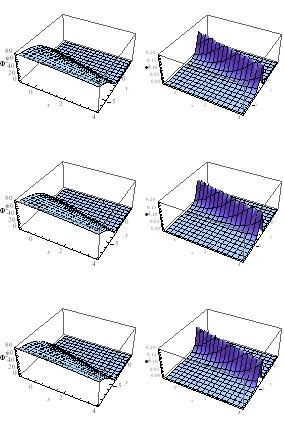
Figure 1: Full anisotropy (left) and the lowest-order WKB approximation (right) in the probability density corresponding to the wave functions to equation (42) and (52), respectively, considering the anisotropic variables $\rm(x,y)\to(\beta_{+},\beta_{-})$, centering in $\Omega=-2,0$ and 2, beginning in the up to down in the graphics. The numerical order $\frac{1}{18}$ is considered for the value $Q=-\frac{2}{3}$ and the constant $\rm\mu^{2}=0$ appeared in the Bohm’s formalism.

VI Final Remarks

In this work we have explored a compactification of a ten-dimensional gravity theory coupled with a time-dependent dilaton into a time-dependent six-dimensional torus. The effective theory which emerges through this process resembles in the Einstein frame was applied to anisotropic cosmological Bianchi type II model. By incorporating the matter content and by using the analytical procedure of Hamilton equation of classical mechanics, in appropriate coordinates, we found the classical solution for the anisotropic Bianchi type II cosmological model. In the quantum formalism for the standard Wheeler-DeWitt equation, we can observe that this anisotropic model is completely integrable without employ numerical methods, similar solutions to partial differential equation have been found in SOCORRO2010 . In order to have the best candidates for quantum solutions become those that have a damping behavior with respect to the scale factor, represented in our model with the $\Omega$ parameter, in this way we dropped in the full solution the modified Bessel function $\rm I_{\nu}(z)$ and the term $\rm e^{S}$ in the Bohm’s solution. We obtain the relation between these both physical solutions in the asymptotic behavior to the modified Bessel function for large argument, (40) and it is compared with the Bohm’s solutions, (52), who us indicate that is the lowest-order WKB approximation how is indicate in the literature sm ; bae . The unnormalized probability density which is shown in the Figure 1, show that the picks of the plot follow the classical trajectory $\beta_{+}=-\sqrt{3}\beta_{-}-|\Omega|$, which corresponds at zero phase in the probability amplitude in both solutions; in other words, this wave function (52) has translational symmetry along the last trajectory mentioned. Also is presented a shifting to the wave function in the $\beta_{-}$ axe in the $-\infty$ direction, that in some sense us indicate that the anisotropy of the model in the quantum state finish for large $+\beta_{-}$ and follow this in the line $\beta_{+}=-\sqrt{3}\beta_{-}-|\Omega|$ .

For future work is to consider a more complete compactification process in which all moduli are considered as time-dependent fields as well as time-dependent fluxes and follow the analysis presented in the ref. bae to obtain the other orders to the WKB approximation, and see how these orders contribute to the full solution found by separation of variables.

References

• (1) T. Damour and A.M. Polyakov, Nucl. Phys. B 423, 532 (1994).
• (2) J. Horne and G. Moore, Nucl. Phys. B 432, 109 (1994).
• (3) T. Banks, M. Berkooz, S.H. Shenker, G. Moore, and P.J. Steinhardt, Phys. Rev. D 52, 3548 (1995).
• (4) T. Damour, M. Henneaux, B. Julia and H. Nicolai, Phys. Lett. B 509, 323 (2001).
• (5) T. Banks, w. Fischler and L. Motl, J. High Energy Phys. 01, 091 (1999).
• (6) R. Kallosh, L. Kofman and A.D. Linde, Phys. Rev. D 64, 123523 (2001).
• (7) R. Kallosh, L. Kofman, A. Linde and A. Tseytlin, Phys. Rev. D 64, 123524 (2001).
• (8) D. Baumann and Liam McAllister, arXiv:1404.2601 [hep-th], Inflation and String Theory .
• (9) J. Khoury, B.A. Ovrut, N. Seiberg, P.J. Steinhardt and N. Turok, Phys. Rev. D 65, 086007 (2002)
• (10) K. Enqvist, e. Keski-Vakkuri and S. Räsänen, Nucl. Phys. B 614, 388 (2001); and references therein.
• (11) G. Veneziano, Phys. Lett. B 265, 287 (1991).
• (12) C.J. Isham, Canonical Quantum Gravity and the Problem of time, in Integrable Systems, Quantum Groups and Quantum Field Theories (Kluwer Academic Publishers, London 1992).
• (13) K.V. Kuchar, Time and Interpretations of Quantum Gravity, in Proceedings of the 4th Conference on General Relativity and Relativistic Astrophysics, eds. G. Kunstatter, D. Vincent and J. Williams (World Scientific, Singapore 1992).
• (14) M. Aguero, J.A.S. Aguilar, C. Ortiz, M. Sabido and J. socorro, Int. J. of Theor. Phys. 46, 2928 (2007).
• (15) O. Obregón, J. Socorro and J. Benítez, Phys. Rev. D 47, 4471 (1993), and references therein.
• (16) C. Brans and R.H. Dicke, Phys. Rev. 124, 925(1961).
• (17) M.P Ryan and L.C. Shepley, Homogeneous Relativistic Cosmologies (Princenton), (1975).
• (18) J. Socorro, Int. J. of Theor. Phys. 42, 2087 (2003).
• (19) Borun D. Chrowdhury and Samir D. Mathur, Class. Quant. Grav. 24, 2689 (2007), Fractional Brane State in Early Universe.
• (20) S. Nojiri, O. Obregón, S.D.Odintsov and K.E. Osetrin. Phys. Rev. D 60, 024008 (1999). (Non) Singular Kantowski-Sachs Universe from Quantum Spherically.
• (21) S. Nojiri, O. Obregón, S.D. Odintsov and K.E. Osetrin. Phys. Lett. B 449, 173 (1999), Induced Wormholes due to Quantum Effects of Spherically Reduced Matter in Large N Approximation.
• (22) G.W. Gibbons and L. P. Grishchuk Nucl. Phys. B 313, 736 (1989).
• (23) Li Zhi Fang and Remo Ruffini, Editors, Quantum Cosmology, Advances Series in Astrophysics and Cosmology Vol. 3 (World Scientific, Singapore, 1987).
• (24) J.B. Hartle and S.W. Hawking, Phys. Rev. D 28, 2960 (1983).
• (25) S.W. Hawking Nucl. Phys. B 239, 257 (1984).
• (26) P.V. Moniz, Quantum cosmology -the supersymmetric perspective- Vol. 1 & 2, Lecture Notes in Physics 803 & 804, (Springer, Berlin) (2010).
• (27) J. H. Bae, Class. Quantum Grav. 32, 075006 (2015). Mixmaster revisited: wormhole solutions to the Bianchi IX Wheeler DeWitt equation using the Euclidean-signature semiclassical method
• (28) D. Bohm, Phys. Rev. 85, 166 (1986).
• (29) J. Socorro, Paulo A. Rodríguez, O. Núñez-Soltero, Rafael Hernández and Abraham Espinoza-García, Open questions in cosmology, Intech, Chapter 9, Quintom Potential from Quantum Anisotropic Cosmological Models, pag 219. Edited by Gonzalo J. Olmo, (2012).
• (30) R. Graham, Phys. Rev. Lett. 67, 1381 (1991).
• (31) C.V. Sukumar, J. Phys. A 18, 2917 (1985).
• (32) O. Obregón and J. Socorro, Int. J. of Theor. Phys. 35 (7), 1381 (1996).
• (33) W. Guzmán, M Sabido, J. Socorro and L. Arturo Ureña-López, Int. J. Mod. Phys. D 16 (4), 641 (2007).
• (34) J. Socorro and E.R. Medina, Phys. Rev. D 61, 087702 (2000), Supersymmetric quantum mechanics for Bianchi Class A models
• (35) J. Socorro, M. Sabido, M.A. Sánchez, and M.G. Frías Palos, Revista Mexicana de Física 56, 166 (2010), Anisotropic cosmology in Sáez-Ballester theory: classical and quantum solutions.
• (36) K. Peeters, [hep-th/0701238], Introducing Cadabra: A Symbolic computer algebra system for field theory problems, (2007).
• (37) K. Peeters, [abs/cs/0608005], A field-theory motivated approach to symbolic computer algebra, (2006).