Extending the applicability of Redfield theories into highly non-Markovian regimes

Abstract

We present a new, computationally inexpensive method for the calculation of reduced density matrix dynamics for systems with a potentially large number of subsystem degrees of freedom coupled to a generic bath. The approach consists of propagation of weak–coupling Redfield–like equations for the high frequency bath degrees of freedom only, while the low frequency bath modes are dynamically arrested but statistically sampled. We examine the improvements afforded by this approximation by comparing with exact results for the spin–boson model over a wide range of parameter space. The results from the method are found to dramatically improve Redfield dynamics in highly non–Markovian regimes, at a similar computational cost. Relaxation of the the mode–freezing approximation via classical (Ehrenfest) evolution of the low frequency modes results in a dynamical hybrid method. We find that this Redfield–based dynamical hybrid approach, which is computationally more expensive than bare Redfield dynamics, yields only a marginal improvement over the simpler approximation of complete mode arrest.

I Introduction

Useful approximate methods for the description of quantum dynamics and relaxation can often circumvent the large computational expense of numerically exact approaches while maintaining quantitative accuracy in certain regions of parameter space. The general applicability of such methods, however, is often limited and their domain of validity difficult to assess. The most widely used approximate approaches fall into two broad and general classes. The first class of methods involves techniques that employ uncontrolled approximations to yield dynamics which are non–perturbative in the various couplings (e.g., intra–system or system–bath) that characterize the problem. The second class of methods are systematically perturbative in a well–defined coupling parameter, but are free from further classical or semiclassical approximations, at least for simply defined models such as a the spin–boson model.

One of the most celebrated perturbative techniques is a lowest–order treatment of the system–bath coupling, known traditionally as Redfield theory.Bloch (1957); Redfield (1965); Nitzan (2006) As we will show later, the relevant dimensionless parameter characterizing the accuracy of Redfield theory is $\eta=\mathrm{max}\left[2\lambda/\beta\omega_{c}^{2},2\lambda/\pi\omega_{c}\right]$, where $\lambda$ is the nuclear reorganization energy, $\beta=1/k_{B}T$ is the inverse temperature, and $\omega_{c}$ is a characteristic bath frequency (we henceforth work in units with $\hbar=1$). Redfield theory becomes unreliable when $\eta\gtrsim 1$. We emphasize that $\eta$ is controlled by multiple bath parameters and, in particular, low frequency degrees of freedom (small $\omega_{c}$) limit the range of accessible reorganization energies. Indeed, violations of this condition explain the failures of Redfield theory found by Ishizaki and FlemingIshizaki and Fleming (2009a) for certain models of excitation energy transfer, which appear to be characterized by low–frequency protein baths.

While the very lowest frequency degrees of freedom are thus most problematic for Redfield theory to handle (even in its non–Markovian forms), it is often the case that nuclear modes of such frequencies are effectively frozen on the time scale of relevance for the system’s dynamics. In this regard, the key function of such modes is simply to provide static energetic disorder for the more rapidly evolving degrees of freedom. This suggests a methodology whereby the very low frequency phonons are approximated as static (and treated non–perturbatively as a source of static disorder), while the remaining portion of the bath is treated dynamically within Redfield theory. Here we develop this “Redfield theory with frozen modes” (Redfield–FM) method, and show that it greatly extends the applicability of Redfield theory into highly non–Markovian dynamical regimes at essentially no change in computational cost.

The outline of this paper is as follows. In Sec. II, we introduce the theoretical background for the Redfield equations and the derivation and general properties of the Redfield–FM extension. In addition, we also introduce the spin–boson Hamiltonian as the model system on which we test the methods developed in this paper. Section III.1 presents the computational details in the implementation of the Redfield–FM method, while Sec. III.2 presents illustrative results for the method. In Sec. III.3, we relax the mode–freezing approximation via the derivation and implementation of a dynamical hybrid method (hybrid–Redfield) that combines Redfield dynamics for the high–frequency part of the bath coupled to the electronic system and Ehrenfest dynamics for the low–frequency modes. In Sec. IV, we conclude.

II Theory

II.1 Model

First, we briefly describe the model system we use to test the approximations developed in subsequent sections. This allows us to define notation and parameters that will be used in our numerical comparisons. We focus on the well–known spin–boson model, which consists of a two–level system coupled linearly to a harmonic bath. This model has been extensively used to investigate a wide variety of relaxation, charge and energy transport processes in condensed phase systems.Weiss (1999)

The total Hamiltonian is divided into system, bath, and interaction components, $H=H_{\mathrm{sys}}+H_{\mathrm{bath}}+V$. The system Hamiltonian takes the form

$$H_{\mathrm{sys}}=\varepsilon\sigma_{z}+\Delta\sigma_{x},$$ (1)

where $\sigma_{i}$, $i=\{x,y,z\}$, are the Pauli matrices, $2\varepsilon$ is the energy difference, and $\Delta$ is the coupling between the two electronic sites, which is here assumed to be static. The bath Hamiltonian consists of an infinite set of harmonic oscillators,

$$H_{\mathrm{bath}}=\sum_{k}\frac{1}{2}\left[P_{k}^{2}+\omega_{k}^{2}Q_{k}^{2}\right].$$ (2)

Lastly, the system–bath interaction couples the electronic states linearly to coordinates of the bath oscillators,

$$V=\sigma_{z}\sum_{k}c_{k}Q_{k}.$$ (3)

Physically, the system–bath coupling acts as a (quantum) fluctuating field that shifts the origin of the bath harmonic oscillators by a magnitude that depends on the system’s electronic state and the strength of the coupling.

The spectral density, which completely determines the coupling between the bath and the system, is taken to be Ohmic with a Lorentzian cutoff (Debye form),

$$J(\omega)=\frac{\pi}{2}\sum_{k}\frac{c_{k}^{2}}{\omega_{k}}\delta(\omega-\omega_{k})=2\lambda\omega_{c}\frac{\omega}{\omega^{2}+\omega_{c}^{2}}.$$ (4)

The cutoff frequency, $\omega_{c}$, characterizes how quickly the bath relaxes toward equilibrium, while the reorganization energy, $\lambda=\pi^{-1}\int_{0}^{\infty}d\omega\ J(\omega)/\omega$, characterizes the energy dissipated by the environment after a Franck–Condon transition between electronic states. It is important to note that the methods studied here are neither limited to the spin–boson model nor to the Debye form for the spectral density.

II.2 Time–local Redfield Dynamics

Because of its simplicity in the time domain we employ the time–local (i.e. time–convolutionless) form of the generalized Redfield equations. A full derivation of these equations is contained in Appendix A. Here our aim is to highlight important but often overlooked aspects pertaining to the applicability of the Redfield approach. For the spin–boson model, the time–local version of the Redfield theory takes the following form,

$$\begin{split}\frac{d}{dt}\rho(t)&=-i\left[H_{\mathrm{sys}},\rho(t)\right]\\ &\hskip 10.00002pt-\int_{0}^{t}d\tau\ \Big{\{}C(\tau)\left[\sigma_{z}(0),\sigma_{z}(-\tau)\rho(t)\right]\\ &\hskip 50.00008pt-C^{*}(\tau)\left[\sigma_{z}(0),\rho(t)\sigma_{z}(-\tau)\right]\Big{\}},\end{split}$$ (5)

where all operators except the reduced density matrix (RDM) are evolved in the interaction picture, $O(t)=e^{-i(H_{\mathrm{sys}}+H_{\mathrm{bath}})t}Oe^{i(H_{\mathrm{sys}}+H_{\mathrm{bath}})t}$, and the free bath correlation function is given by

$$\begin{split}C(t)&=\sum_{k}c_{k}^{2}\operatorname{Tr}_{\mathrm{bath}}\Big{\{}\rho_{\mathrm{bath}}Q_{k}(t)Q_{k}(0)\Big{\}}\\ &=\frac{1}{\pi}\int_{0}^{\infty}d\omega J(\omega)[\coth(\beta\omega/2)\cos(\omega t)-i\sin(\omega t)].\end{split}$$ (6)

By going to the interaction picture with respect to $H_{\mathrm{sys}}+H_{\mathrm{bath}}$ (to eliminate the free-evolution) and formally integrating the equation of motion (5), one finds

$$\rho_{I}(t)=\rho_{I}(0)\left[1+O\left(\int_{0}^{t}d\tau_{1}\int_{0}^{\tau_{1}}d\tau_{2}\ C(\tau_{2})\right)+\dots\right].$$ (7)

Examination of the function $\int_{0}^{t}d\tau_{1}\int_{0}^{\tau_{1}}d\tau_{2}\ C(\tau_{2})$ reveals the natural dimensionless parameter that determines the limit of validity of Redfield theory. In general, even in the non–Markovian case, we expect that the ordering of terms in the expansion (7) is governed by the function $\int_{0}^{t}d\tau_{1}\int_{0}^{\tau_{1}}d\tau_{2}\ C(\tau_{2})=\eta g(t)$, where $\eta$ is a dimensionless constant and $g(t)$ is a function expressed in terms of a scaled, dimensionless time variable. In the high–temperature limit ($\beta\omega_{c}\ll 1$), where $C(t)\approx(2\lambda/\beta)e^{-\omega_{c}t}$, it is easy to show

$$\eta =2\lambda/(\beta\omega_{c}^{2})$$ (8a)

$$g(t) =e^{-\omega_{c}t}-1+\omega_{c}t.$$ (8b)

In the low–temperature limit ($\beta\omega_{c}\gg 1$), we assume that the low–frequency behavior of the spectral function dominates, so we choose $J(\omega)=(2\lambda\omega/\omega_{c})e^{-2\omega/\pi\omega_{c}}$ as an approximation to the Debye form in Eq. (4) that exactly matches the value of $\lambda$ and its low–frequency asymptotic behavior. Using this spectral density, one can show

$$\eta =\frac{2\lambda}{\pi\omega_{c}}$$ (9a)

$$g(t) =\ln\left[1+(\omega_{c}t)^{2}\right]+2\ln\left[\frac{\sinh(\pi t/\beta\hbar)}{(\pi t/\beta\hbar)}\right].$$ (9b)

Thus, for a Debye spectral density, Redfield theory will be reliable as long as $\mathrm{max}\left[2\lambda/\beta\omega_{c}^{2},2\lambda/\pi\omega_{c}\right]$ is not significantly larger than unity. It should be noted that recent work purported to be in the Redfield limit actually violates the above condition.Landry and Subotnik (2015) As long as the relevant energy scales in the system Hamiltonian are not too large, we expect the above to hold. In cases where the system’s bare energy difference $\varepsilon$ is the largest energy scale in the problem, the dynamics will be mediated by multi–phonon processes which are a challenge for lowest–order Redfield–like theories. However, in this limit, the problem acquires an increasing amount of ‘pure–dephasing’ character, for which the time–local version of Redfield theory provides an exact multi–phonon resummation.

II.3 Redfield Theory with Frozen Modes

As discussed in the Introduction, low–frequency bath modes $\omega_{k}$ which lead to a violation of the validity of the Redfield theory frequently evolve so slowly as to be effectively static on the electronic timescale. Here we develop the “Redfield theory with frozen modes” (Redfield–FM) method, based on the physically appealing notion of dividing modes into a low–frequency portion (treated as static disorder), and a high–frequency bath (treated by time–local Redfield theory). The separation of modes used here mirrors that utilized in previous work on a Förster–like dynamical hybrid approach.Berkelbach, Markland, and Reichman (2012) The approach presented here is not in any way limited to time–local Redfield theory (nor even to any specific flavor of Redfield theory). However, due to pathologies associated with a strictly Markovian Redfield theory, we suggest certain adjustments to the partitioning algorithm, as discussed in Appendix B.

First, it is advantageous to assume that the total density matrix is multiplicatively separable into weakly interacting parts, i.e., $\rho_{\mathrm{tot}}(t)\approx\rho_{\mathrm{slow}}(0)\rho_{\mathrm{sys+fast}}(t)$ where $\rho_{\mathrm{slow}}(0)$ is the density matrix of the frozen low–frequency “slow modes” and $\rho_{\mathrm{sys+fast}}(t)$ is the density matrix for the system and high–frequency “fast modes”. As in Ref. Berkelbach, Markland, and Reichman, 2012, a splitting function, $S(\omega)$, divides the spectral density into two components, $J(\omega)=J_{\mathrm{slow}}(\omega)+J_{\mathrm{fast}}(\omega)$, where

$$J_{\mathrm{slow}}(\omega)=S(\omega,\omega^{*})J(\omega),$$ (10)

and

$$J_{\mathrm{fast}}(\omega)=[1-S(\omega,\omega^{*})]J(\omega)$$ (11)

Here we take the same form of the splitting function as that suggested in Ref. Berkelbach, Markland, and Reichman, 2012, namely,

$$S(\omega,\omega^{*})=\left\{\begin{array}[]{lr}[1-(\omega/\omega^{*})^{2}]^{2}&:\quad\omega<\omega^{*}\\ 0&:\quad\omega\geq\omega^{*},\end{array}\right.$$ (12)

which, by virtue of its smoothness, avoids problems associated with long–time oscillatory tails in the bath correlation function.Berkelbach, Reichman, and Markland (2012) While the above splitting induces no errors if the dynamics are treated exactly, it is clear that $\omega^{*}$ serves as a free parameter that allows one to tune the optimum percentage of frozen bath modes, and hence the accuracy of the results if the dynamics are treated within our approximate method. The utility of the present method is greatly enhanced if a physical a priori prescription for choosing $\omega^{*}$ based only on the parameters of the initial Hamiltonian can be put forth. In this work we choose $\omega^{*}=\omega_{R}/4$, where $\omega_{R}=2\sqrt{\varepsilon^{2}+\Delta^{2}}$ is the system Rabi frequency. This choice for $\omega^{*}$ is simple, yields non–trivial improvements over standard Redfield theory, and may easily be generalized to multiple electronic states. Physically, this choice partitions the bath into modes that evolve slower than the system (to be treated as frozen) and modes that evolve faster than the system (to be treated via Redfield theory). However, it should be noted that this choice is not always optimal. Future work will be devoted to the goal of arriving at an optimal choice of $\omega^{*}$. Other choices for $\omega^{*}$ that fit within the general physical guidelines discussed above will be discussed in the Results section.

With a prescription for choosing $\omega^{*}$ in hand, it is possible to separate the fast and slow portions of the Hamiltonian, starting with the interaction, $V_{\mathrm{fast}}=\sigma_{z}\sum_{k\in\mathrm{fast}}c_{k}Q_{k}$ and $V_{\mathrm{slow}}=\sigma_{z}\sum_{k\in\mathrm{slow}}c_{k}Q_{k}$. Regrouping terms, it is evident that freezing the slow part, $V_{\mathrm{slow}}$, will yield a classical reorganization energy that renormalizes the bias for every realization of the bath’s initial conditions. The modified total Hamiltonian now takes the following form,

$$\begin{split}H^{\prime}&=[\varepsilon+\lambda^{cl}(0)]\sigma_{z}+\Delta\sigma_{x}\\ &+\sigma_{z}\sum_{k\in\mathrm{fast}}c_{k}Q_{k}+\frac{1}{2}\sum_{k}\Big{[}P_{k}^{2}+\omega_{k}^{2}Q_{k}^{2}\Big{]},\end{split}$$ (13)

where the classical reorganization energy is defined as $\lambda^{cl}(0)=\sum_{k\in\mathrm{slow}}c_{k}Q_{k}(0)$ and the set of $Q_{k}(0)$ is sampled from a bath distribution function after the discretization of $J_{\mathrm{slow}}(\omega)$. Physically, each realization of the frozen bath degrees of freedom constitutes a local, rigid environment that modifies the site energies for the system Hamiltonian. The time–local Redfield dynamics, under the Hamiltonian in Eq. (13) with an interaction given by $V_{\mathrm{fast}}=\sigma_{z}\sum_{k\in\mathrm{fast}}c_{k}Q_{k}$, are subsequently ensemble averaged with respect to the slow frozen modes. Thus, there are two important differences for the Redfield equations used in each realization of the frozen modes: (i) the bias is given by $\tilde{\varepsilon}\equiv\varepsilon+\lambda^{cl}(0)$, and (ii) the bath correlation function given by Eq (6) is modified, with $J(\omega)$ replaced by $J_{\mathrm{fast}}(\omega)$.

To account for the classical frozen modes, the nonequilibrium population dynamics takes the following form,

$$\langle\sigma_{z}(t)\rangle\approx\int d\mathbf{P}d\mathbf{Q}\ \rho_{\mathrm{slow}}(\mathbf{P},\mathbf{Q},0)\operatorname{Tr}_{\mathrm{sys+fast}}[\rho_{\mathrm{sys+fast}}(t)\sigma_{z}],$$ (14)

where $\rho_{\mathrm{slow}}(\mathbf{P},\mathbf{Q},0)$ could be either the classical distribution function or the Wigner transform of the equilibrium density operator of the slow bath degrees of freedom, and $\rho_{\mathrm{sys+fast}}(t)$ is the reduced density matrix of the system and the fast bath degrees of freedom. Observables such as $\operatorname{Tr}_{\mathrm{sys+fast}}[\rho_{\mathrm{sys+fast}}(t)\sigma_{z}]$ may then be calculated via the Redfield equations.

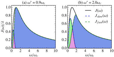
Figure 1: Spectral density and splitting via $S(\omega,\omega^{*})$, illustrating the two situations expressed in Eqs. (10) and (11).

To understand the relaxation processes with mode freezing for finite $\omega^{*}$, it is first useful to investigate the effect of the approximation at its most extreme, namely the adiabatic limit, where all bath modes are assumed to be static ($\omega^{*}\rightarrow\infty$). In this limit, we are effectively in the Born–Oppenheimer regime, where excitations in the electronic subspace move along the potential energy surface determined by the frozen reservoir. Analytical evaluation of the trace within Eq. (14) leads to the following expression for the nonequilibrium population dynamics,

$$\langle\sigma_{z}(t)\rangle\approx\int d\mathbf{P}d\mathbf{Q}\ \rho_{\mathrm{bath}}(\mathbf{P},\mathbf{Q},0)\ \frac{\tilde{\varepsilon}^{2}+\Delta^{2}\cos(\xi t)}{\tilde{\varepsilon}^{2}+\Delta^{2}},$$ (15)

where $\xi=2\sqrt{\tilde{\varepsilon}^{2}+\Delta^{2}}$ is the Rabi frequency of the modified system Hamiltonian. The integration over the ensemble of equilibrium configurations of the bath reduces to averaging over different values of $\lambda^{cl}(0)$ that are consistent with the bath distribution function. For some realizations of the bath, Eq. (15) recovers the Rabi oscillations characteristic of the isolated system if $\lambda^{cl}(0)=0$. Conversely, when $\lambda^{cl}(0)\neq 0$, the population starts from 1 at $t=0$ and will oscillate between $(\tilde{\varepsilon}^{2}+\Delta^{2})/(\tilde{\varepsilon}^{2}+\Delta^{2})=1$ and $(\tilde{\varepsilon}^{2}-\Delta^{2})/(\tilde{\varepsilon}^{2}+\Delta^{2})$. Taking for simplicity $\varepsilon=0$, one notes that the lower bound of the population oscillations increases with increasing $\lambda^{cl}(0)$, approaching 1 as $\lambda^{cl}(0)\rightarrow\infty$. This limit corresponds to an infinitely rigid bath that completely localizes the excitation on its initial site.

Averaging over different realizations of the slow modes decreases the amplitude of oscillations in the population dynamics due to the decoherence between the functions with distinct oscillation frequencies. In general, Redfield theory has difficulty describing non–Markovian, multi–step relaxation dynamics. However, when $\lambda_{\mathrm{slow}}=\pi^{-1}\int_{0}^{\infty}d\omega\ J_{\mathrm{slow}}(\omega)/\omega$ is sufficiently large, the full dynamics produced by Redfield theory with frozen modes at finite $\omega^{*}$ will include both a slow, perhaps oscillatory component as well as a more rapid decay induced by the high frequency modes in $J_{\mathrm{fast}}(\omega)$. These qualitative considerations suggest this approach may correct certain deficiencies of conventional Redfield–like approaches. In the next section, we test the approach quantitatively.

III Results

In the following, we compare the numerically exact population dynamics reported by Thoss et al.Thoss, Wang, and Miller (2001) for the spin–boson model with a Debye spectral density and the initial condition $\Gamma(0)=\ket{1}\bra{1}\exp(-\beta H_{\mathrm{bath}})/Z_{\mathrm{bath}}$ with the results obtained from the Redfield–FM method. Subsequently, we examine the effect of relaxing the mode–freezing approximation by treating the low–frequency modes dynamically via the Ehrenfest method. We call this latter approach the hybrid–Redfield method, in analogy with the previously developed hybrid–NIBA method.Berkelbach, Reichman, and Markland (2012); Berkelbach, Markland, and Reichman (2012)

III.1 Computational Details

To treat the frozen portion of the spectral density, $J_{\mathrm{slow}}(\omega)$, we have discretized the bath into $f=300$ modes with frequencies and couplings given byCraig and Manolopoulos (2005); Berkelbach, Reichman, and Markland (2012)

$$\omega_{k}=\omega_{c}\tan\Bigg{[}\frac{\pi}{2f}(k-1/2)\Bigg{]},$$ (16)

and

$$c_{k}^{2}=\frac{2\lambda}{f}\omega_{k}^{2}.$$ (17)

Initial conditions for the reservoir of frozen modes were sampled from a Wigner distribution. Sampling from this distribution becomes particularly important at very low temperatures, where quantum effects become significant. However, for most cases, sampling from a Boltzmann distribution is sufficient since the modes being samples are always low–frequency. For convergence, up to $10^{4}$ trajectories have been run for the results presented.

III.2 Redfield–FM Method

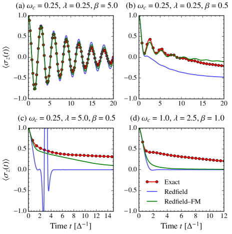
Figure 2: Results from Redfield–FM approach compared with standard time–local Redfield theory and exact numerics. $\omega^{*}=\mathrm{max}[\omega_{c},\frac{\omega_{R}}{4}]$ and $\omega_{R}=2\sqrt{\Delta^{2}+\epsilon^{2}}$. All units are scaled by the electronic coupling $\Delta$. All panels correspond to unbiased cases ($\varepsilon=0$), except for panel (b), where $\varepsilon=1.0$. Other parameters are stated in the panels.

As mentioned in Sec. II.2, the validity of Redfield theory is limited to the small $\eta$ regime. Fig. 2(a) shows the results for a slow bath ($\omega_{c}=0.25$) with small reorganization energy ($\lambda=0.25$) at low temperature ($\beta=5.0$); here and in the following, all energies are in units of $\Delta$. In spite of the slow bath, the dimensionless applicability parameter is only slightly larger than unity ($\eta=1.6$) suggesting that Redfield theory should be reasonably accurate, in agreement with the numerical results. The Redfield–FM method provides an even better estimate of the dynamics, almost quantitatively correcting the already accurate Redfield dynamics.

Fig. 2(b) considers a biased system ($\varepsilon=1.0$) with the same parameters, except at much higher temperature ($\beta=0.5$), yielding an applicability parameter which is now significantly larger than unity ($\eta=16$). Here, it is evident that the Redfield dynamics relax far too quickly, suppressing the coherence and missing the slower relaxation process revealed by the exact dynamics. The improvement afforded by the Redfield–FM method compared to standard Redfield theory is clear. In particular, the Redfield–FM approach accurately reproduces the short– to intermediate–time dynamics, the frequency of the oscillations, and the initial rate of decoherence. The terminal decay rate is slightly underestimated due to the mode–freezing approximation, as discussed in Section II.B. Yet despite these shortcomings, the improvement derived from a simple scheme like the Redfield–FM approach with the numerical complexity of the original Redfield theory is noteworthy.

For cases exemplified by Fig. 2(c), serious problems such as the violation of the positivity of the RDM dynamics can occur within standard (non–secular) Redfield theory. Figure 2(c) corresponds to a slow bath ($\omega_{c}=0.25$) and a large reorganization energy ($\lambda=5.0$) again at high temperature ($\beta=0.5$), for which the applicability parameter is very large ($\eta=320$). Despite the evident failure of the Redfield equations to even maintain positivity, the Redfield–FM method is able to correct the positivity issue and almost quantitatively reproduce the two–step relaxation process in the exact dynamics up to intermediate times.

It is possible to understand the surprising success presented in Fig. 2(c) in the context of the analysis of Section II.B. Using the definitions given in that section, the effective parameters for the Redfield equation are $\lambda_{\mathrm{fast}}=2.5$, $\omega_{c}=0.5$, yielding $\eta=40$. Although $\eta\gg 1$, the reduction by an order of magnitude from the initial value, $\eta=320$, is sizeable, and likely responsible for solving the positivity problem evident in the bare Redfield dynamics. The reproduction of the two–step relaxation process is a direct result of the trapping effect that arises from freezing a large portion of the low–frequency bath in the presence of large coupling. This example indicates that the trapping effect can partially reproduce slow relaxation dynamics associated with strong system–bath interactions.

Figure 2(d) shows the regime of intermediate bath speeds ($\omega_{c}=1$), large reorganization energy ($\lambda=2.5$), and intermediate temperature ($\beta=1$). In contrast to Fig. 1(c), the Redfield–FM method is not capable of significantly improving the Redfield dynamics in this regime, missing the two–step relaxation process visible in the exact dynamics. In light of the previous case, it is evident that the slowing down of the RDM dynamics can be caused by freezing a large portion of the strongly coupled modes, an effect which is absent in this case. In this case, $\lambda_{\mathrm{fast}}=2.1$ and $\lambda_{\mathrm{slow}}=0.4$, which indicates that most of the reorganization energy is included already in the high–frequency portion of the bath. In such cases, the Redfield–FM method will yield results that are similar to bare Redfield theory.

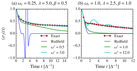
Figure 3: Redfield–FM results for $\omega^{*}=\mathrm{max}[\omega_{c},\frac{\omega_{R}}{4}]$ and an “optimized” value for $\omega^{*}$. Both cases considered here correspond to $\varepsilon=0$ and all units are scaled by the electronic coupling, $\Delta$. Note that the set of parameters for panels (a) and (b) in this figure correspond to the set of parameters in Fig. 2, panels (c) and (d), respectively.

We now address the dependence of the dynamics on the choice of $\omega^{*}$. Eschewing the simple criteria for choosing $\omega^{*}$ presented above, one may ask how closely the Redfield–FM dynamics can be made to agree with exact dynamics when $\omega^{*}$ is allowed to vary. To address this question, we include two extreme cases in Fig. 3. First, Fig. 3(a), which corresponds to the same parameters as those of Fig. 2(c), shows that optimization of $\omega^{*}$ can result in quantitative agreement between the Redfield–FM result and the exact dynamics. Such agreement may be understood as the result of fortuitous cooperation between strongly dissipative Redfield dynamics that damp the frozen mode–generated oscillations and the trapping effect from the mode–freezing approximation that prevents immediate relaxation to the equilibrium population. Conversely, Fig. 3(b), which corresponds to the parameters in Fig. 2(d), is an example of when perfect agreement is impossible. Clearly, attempts at optimizing $\omega^{*}$ result in better agreement of the two–step relaxation process at the cost of long–lived oscillations, a direct result of including a large fraction of modes into the slow part of the bath. In freezing a sufficiently large portion of the reservoir to reproduce the trapping effect, $\lambda_{\mathrm{fast}}$ is reduced to the point where the Redfield dynamics are no longer sufficiently dissipative to damp the frozen mode–generated oscillations. In addition, $\lambda_{\mathrm{slow}}=\pi^{-1}\int_{0}^{\infty}d\omega J_{\mathrm{slow}}(\omega)/\omega$ is also not large enough to ensure that the oscillations dephase sufficiently rapidly. Overall, it is clear that although it may be possible to optimize the results, the simple initial criteria presented represent a robust approach to frozen mode dynamics that essentially always yields results that are as good or better than bare Redfield dynamics without a significantly increased computational cost.

III.3 Relaxing the Mode–Freezing Approximation: A Dynamical Hybrid Redfield Method

On first inspection, the mode–freezing approximation appears extreme. To thoroughly assess its effect, we develop a dynamical hybrid method in which we evolve the previously frozen low–frequency modes in $J_{\mathrm{slow}}(\omega)$ via classical Ehrenfest dynamics. The derivation and the implementation details of this approach may be found in Appendix C.

This hybrid–Redfield method is similar in spirit to the successful hybrid–NIBA developed and implemented in Ref. Berkelbach, Reichman, and Markland, 2012. Evolution of the low–frequency modes using Ehrenfest dynamics in such hybrid approaches only requires two assumptions: (i) that $\Gamma(t)\approx\rho_{\mathrm{slow}}(t)\rho_{\mathrm{sys+fast}}(t)$, and (ii) that the motion of the low–frequency modes is well–captured by classical mechanics. For such a factorization to be valid, the reorganization energy due to the low–frequency bath needs to be small, i.e., $\lambda_{\mathrm{slow}}=\pi^{-1}\int_{0}^{\infty}d\omega\ J_{\mathrm{slow}}(\omega)/\omega<\Delta$. The applicability of classical dynamics relies on the low energies of the reservoir modes and sufficiently high temperatures that help suppress quantum effects.Stock (1995); Berkelbach, Reichman, and Markland (2012) However, even when the Ehrenfest approximation is valid, problems may arise. Most prominent among these is that the final populations approach those of the infinite–temperature limit.Stock (1995)

In contrast to the Hamiltonian derived under the mode–freezing approximation in Eq. (13), the modified Hamiltonian that needs to be treated via the Redfield equation in the hybrid–Redfield method is time–dependent,

$$\begin{split}H^{\prime\prime}(t)&=[\varepsilon+\lambda^{cl}(t)]\sigma_{z}+\Delta\sigma_{x}\\ &\hskip 10.00002pt+\sigma_{z}\sum_{k\in\text{fast}}c_{k}Q_{k}+\frac{1}{2}\sum_{k}\Big{[}P_{k}^{2}+\omega_{k}^{2}Q_{k}^{2}\Big{]},\end{split}$$ (18)

where the disorder due to the low frequency bath is no longer static as it is in the Redfield–FM method, but rather dynamic, namely $\lambda^{cl}(t)=\sum_{k}c_{k}Q_{k}(t)$.

Since the system part of this Hamiltonian is nondiagonal and time–dependent, evolution with respect to the system Hamiltonian requires diagonalization at every time–step, significantly increasing the computational cost associated with the method proposed here. The need to evolve the low–frequency bath also adds to the computational cost of the approach. Importantly, under the mode–freezing approximation, we circumvent these costly requirements. This means that, aside from the trivial cost of parallelization for the ensemble averaging over the slow bath, the Redfield–FM method scales as gracefully with system size as the original Redfield equation.

For completeness, we remark that the nonequilibrium population dynamics under the hybrid–Redfield approximation now take the form

$$\langle\sigma_{z}(t)\rangle\approx\int d\mathbf{P}d\mathbf{Q}\ \rho_{\mathrm{slow}}(\mathbf{P},\mathbf{Q},t)\operatorname{Tr}_{\mathrm{sys+fast}}[\rho_{\mathrm{sys+fast}}(t)\sigma_{z}].$$ (19)

Fig. 4 shows two sets of parameters for which the hybrid–Redfield scheme yields results that illustrate the issues at play in comparing the hybrid–Redfield approach to the Redfield–FM method. Extensive testing of the hybrid method suggests that an approximately optimal form for the splitting frequency can be taken as

$$\omega^{*}_{hy}=\omega_{R}\lambda/\omega_{c}.$$ (20)

Physically, this form encodes the interplay between the Redfield and Ehrenfest methods, favoring a larger portion of the modes to be treated classically with increasing Rabi frequency $\omega_{R}$, which is a measure of how rapidly the electronic system evolves. Furthermore, this form of $\omega^{*}$ ensures that in the limit of small $\lambda$ and large $\omega_{c}$, the hybrid method correctly reproduces the more appropriate Redfield dynamics, whereas in the limit of large $\lambda$ and small $\omega_{c}$, it reproduces the Ehrenfest results. It is expected that generally nontrivial results may be obtained from this method for cases where $\omega^{*}\sim\omega_{c}$, as is the case for the choice of $\omega^{*}$ used in the Redfield–FM approach.

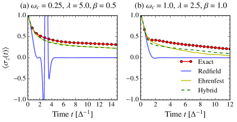
Figure 4: Hybrid–Redfield results for $\omega^{*}_{hy}=\omega_{R}\frac{\lambda}{\omega_{c}}$. Both cases considered here correspond to $\varepsilon=0$ and all units are scaled by the electronic coupling, $\Delta$. Similar to Fig. 3, the set of parameters for panels (a) and (b) in this figure correspond to the set of parameters in Fig. 2, panels (c) and (d), respectively.

Fig. 4(a) corresponds to the parameters in Fig. 2(c) and illustrates that, by means of the suggested form for $\omega^{*}$, hybrid–Redfield automatically tunes itself to yield nearly optimal results achievable from the two parent methods. This example, for which $\omega^{*}_{hy}\gg\omega_{c}$, illustrates that the hybrid–Redfield method trivially reproduces the Ehrenfest result when it is appropriate. It is noteworthy that the Redfield–FM method obtains similar agreement at a much lower computational cost without evolving the reservoir modes, indicating that dynamic treatment of these modes may not be generally necessary. Indeed, it is rather remarkable that the Redfield–FM approach basically recapitulates the Ehrenfest results even though no Ehrenfest dynamics are used.

Fig. 4(b) shows the analogue of Fig. 2(d), where the Redfield–FM method fails to correct the Redfield dynamics. In contrast, the hybrid–Redfield results are in very good agreement with the exact dynamics. Indeed, the hybrid method is able to qualitatively and almost quantitatively reproduce the shape of the two–step relaxation process evident in the exact dynamics, an effect that both Ehrenfest and Redfield dynamics independently miss.

As the above considerations indicate, there are cases where the dynamical hybrid–Redifeld method can provide a substantial improvement over the Redfield–FM method, albeit at a much higher computational cost. In most regions of parameter space we have studied, however, we find that hybrid–Redfield theory offers little accuracy gain over the Redfield–FM approach. Thus, the benefits of the hybrid–Redfield approach compared to the Redfield–FM method do not justify its use when accuracy and cost are factored together.

IV Conclusions

In this work, we have presented a new scheme for simulating dynamics in quantum dissipative systems. Our approach, which we call the Redfield–FM method, recognizes that standard Redfield theory becomes inaccurate for slow bath degrees of freedom. By partitioning the bath into high– and low–frequency components, we propose solving the Redfield equations for the high–frequency partition in the statically disordered field of the low–frequency components. Such an approach may greatly increase the accuracy of Redfield theory in highly non–Markovian regimes at essentially the same computational cost. In addition, we find that this simple approach can fundamentally cure positivity problems associated with standard non–secular Redfield theory. We have further discussed a scheme (the hybrid–Redfield approach) whereby the previously frozen degrees of freedom are instead evolved with classical Ehrenfest dynamics. While this method can improve upon the dynamics as described by the Redfield–FM approach, the increase in accuracy is incremental and comes at a significantly larger computational cost. Overall, while the Redfield–FM method does not cure all of the ills of Redfield theory, it does provide a simple and efficient framework for improving its accuracy and range of validity, especially for sluggish bath degrees of freedom such as those implicated in biological energy transfer.

Appendix A Derivation of Redfield equations

Here, for completeness, we review the derivation of the Redfield equations. For a more detailed discussion of Redfield theory, we refer the reader to Refs. Breuer and Petruccione, 2002 and Chang and Skinner, 1993.

In the following development we utilize a projection operator technique to derive an equation of motion for the reduced density matrix (RDM) of the system, defined as $\rho(t)=\operatorname{Tr}_{\mathrm{bath}}[\Gamma(t)]$, where $\Gamma(t)=e^{-iHt}\Gamma(0)e^{iHt}$ and $\Gamma(0)$ is the initial density matrix of the full system and bath. Moreover, we assume that the initial condition for the (total) density matrix contains no system–bath correlation, such that $\Gamma(0)=\rho(0)\rho_{\mathrm{bath}}$, where $\rho(0)$ is an arbitrary Hermitian system operator, $\rho_{\mathrm{bath}}=e^{-\beta H_{\mathrm{bath}}}/Z$, $Z=\operatorname{Tr}_{\mathrm{bath}}[e^{-\beta H_{\mathrm{bath}}}]$ and $\beta=1/k_{B}T$ is the thermal energy. Treatment of general initial conditions is also possible via the projection operator technique at the expense of the introduction of additional inhomogeneous terms in Eq. (5).Zwanzig (1961); Jang, Cao, and Silbey (2002); Shibata and Arimitsu (1980) In the following, we ignore initial correlations, but note that their inclusion in the present framework is straightforward.

We start from the Liouville equation for the full density matrix in the interaction picture where the total Hamiltonian is divided into a zeroth order part and an interaction part, $H=H_{0}+H_{1}$, such that

$$\frac{d}{dt}\Gamma_{I}(t)=-i\mathcal{L}_{I}(t)\Gamma_{I}(t),$$ (21)

$\Gamma_{I}(t)=e^{iH_{0}t}\Gamma(t)e^{-iH_{0}t}$ and $\mathcal{L}_{I}(t)=[e^{-iH_{0}t}H_{1}e^{iH_{0}t},...]$. To obtain the dynamics of the RDM, we define a projection operator of form $\mathcal{P}\equiv\rho_{\mathrm{bath}}\operatorname{Tr}_{\mathrm{bath}}[...]$ with $Q\equiv 1-\mathcal{P}$. We note that action of $\mathcal{P}$ on the full density matrix followed by trace over the bath results in the RDM in the interaction picture, $\rho_{I}(t)=\operatorname{Tr}_{\mathrm{bath}}[\mathcal{P}\Gamma_{I}(t)]$. Using these definitions, we obtain the following exact equations of motion,

$$\frac{d}{dt}\mathcal{P}\Gamma(t) =-i\mathcal{P}\mathcal{L}_{I}(t)(\mathcal{P}+\mathcal{Q})\Gamma(t)$$ (22)

$$\frac{d}{dt}\mathcal{Q}\Gamma(t) =-i\mathcal{Q}\mathcal{L}_{I}(t)(\mathcal{P}+\mathcal{Q})\Gamma(t).$$ (23)

Formal integration of Eq. (23) yields

$$\mathcal{Q}\Gamma_{I}(t)=-i\int_{0}^{t}d\tau\ g(t,\tau)\mathcal{Q}\mathcal{L}_{I}(t)\mathcal{P}\Gamma_{I}(\tau),$$ (24)

where $g(t,\tau)=\exp_{+}[-i\int_{\tau}^{t}ds\ \mathcal{Q}\mathcal{L}_{I}(s)]$ and the time ordering ($+$) implies that time arguments increase from right to left. Substitution of this expression in Eq. (21) results in the Nakajima–Zwanzig equation,Zwanzig (1961); Jang, Cao, and Silbey (2002) which is expressed in terms of the time convolution of a memory term with $\rho_{I}(t)$ at earlier times as

$$\frac{d}{dt}\rho_{I}(t)=-\int_{0}^{t}d\tau\ K(t-\tau)\rho_{I}(\tau),$$ (25)

where $K(t-\tau)=\operatorname{Tr}_{\mathrm{bath}}[\mathcal{L}_{I}(t)g(t,\tau)\mathcal{Q}\mathcal{L}_{I}(\tau)\rho_{\mathrm{bath}}]$ is the (time–nonlocal) memory function.

If, instead, we use the formal solution of Eq. (21) to evolve $\Gamma_{I}(t)$ backwards in time to an earlier time $\tau$, we obtain

$$\Gamma_{I}(\tau)=G(t,\tau)\Gamma_{I}(t),$$ (26)

where $G(t,\tau)=\exp_{-}[i\int_{\tau}^{t}ds\mathcal{L}_{I}(s)]$ and the time ordering ($-$) requires that time arguments increase from left to right. Replacing this expression in Eq. (24) and solving for $\mathcal{Q}\Gamma_{I}(t)$ yields

$$\mathcal{Q}\Gamma_{I}(t)=[1-\Sigma(t)]^{-1}\Sigma(t)\mathcal{P}\Gamma_{I}(t),$$ (27)

where

$$\Sigma(t)=-i\int_{0}^{t}d\tau\ g(t,\tau)\mathcal{Q}\mathcal{L}(\tau)\mathcal{P}G(t,\tau).$$ (28)

We note that a crucial requirement for the validity of this derivation is the existence of $[1-\Sigma(t)]^{-1}$.

Substitution of Eq. (27) into Eq. (21) and subsequent trace over the bath degrees of freedom results in the following time–local equation of motion for the RDM,Shibata and Arimitsu (1980)

$$\frac{d}{dt}\rho_{I}(t)=R(t)\rho(t),$$ (29)

where $R(t)=-i\operatorname{Tr}_{\mathrm{bath}}[\mathcal{L}_{I}(t)[1-\Sigma(t)]^{-1}\rho_{\mathrm{bath}}]$ is the (time–local) rate function.

The expression for the dynamical evolution in either the time–nonlocal (Eq. (25)) or time–local (Eq. (29)) form is exact but prohibitively difficult to evaluate without resorting to approximation schemes, such as truncated generalized cumulant expansions. Perturbative expansion to second order in the system–bath coupling (where $H_{1}=V$ from Eq. (3)) results in a non–Markovian generalization of the Redfield theory. Alternatively, one may derive both forms of the Redfield equations via resummations of differently time–ordered cumulants.Yoon, Deutch, and Freed (1975); Mukamel, Oppenheim, and Ross (1978) These derivations explicitly show that both forms of generalized Redfield theory account for non–Markovian behavior and have similar applicability requirements.Mukamel, Oppenheim, and Ross (1978); Breuer, Kappler, and Petruccione (1999); Coalson and Evans (2004) Specifically, since Redfield theory is tantamount to second–order perturbation theory in the system–bath coupling, truncation at low order is only accurate for $\eta<1$, where $\eta=\mathrm{max}[\frac{2\lambda}{\beta\omega_{c}^{2}},\frac{2\lambda}{\pi\omega_{c}}]$ is the validity parameter introduced in Sec. II.2. Despite this restriction, the Redfield equations have been shown to perform surprisingly well, often beyond the small–$\lambda$ and large–$\omega_{c}$ regimes.Yang and Fleming (2002); Palenberg et al. (2001) Nevertheless, for inappropriate regions of parameter space, severe problems can arise, such as violation of positivity in the reduced density matrix.Nitzan (2006)

Appendix B Markovian Redfield theory with Frozen Modes

We wish to consider the performance of the frozen modes method for a strictly Markovian version of Redfield theory, i.e. with a rate tensor $R=R(t\rightarrow\infty)$. In this limit, the time integrals become Fourier–Laplace transforms, such that the Redfield tensor elements can be expressed algebraically in terms of the spectral density $J(\omega)$ evaluated at energy differences $\hbar\omega_{ij}\equiv(E_{i}-E_{j})$.Pollard, Felts, and Friesner (1996); Ishizaki and Fleming (2009b) More specifically, we are interested in the dephasing terms of the Redfield tensor, which in general contain an elastic contribution

$$R_{ijij}\sim g_{ij}^{2}\ J(\omega=0+)\ n_{BE}(\omega=0+).$$ (30)

At low frequencies, the Bose–Einstein distribution, $n_{BE}(\omega)\sim kT/\omega$, such that for a spectral density of the form $J(\omega)\sim\omega^{s}$, we find

$$R_{ijij}\sim kT\omega^{s-1}\Big{|}_{\omega=0}.$$ (31)

For all ‘super–Ohmic’ spectral densities with $s>1$, this elastic contribution to the dephasing rate vanishes. However, for an Ohmic spectral density with $s=1$ there is a pure dephasing rate which vanishes only at $T=0$. This contribution to the dephasing rate in the system’s eigenbasis can significantly affect both the population and coherence dynamics in the original basis of the problem.

We now return to the idea of a frozen modes variant of Markovian Redfield theory. Consider specifically an Ohmic spectral density with any non–zero splitting frequency $\omega^{*}$. After partitioning, the fast spectral density has the low–frequency behavior $J_{\mathrm{fast}}(\omega)\sim\omega^{s}$ with $s>1$, which yields no elastic contribution to the dephasing rate. For this reason, a frozen modes version of Markovian Redfield theory does not reduce to the Redfield limit until the singular point $\omega^{*}=0$. Instead, as $\omega^{*}\rightarrow 0$, the result approach a Redfield result which neglects the Ohmic pure dephasing rate. We emphasize that the time–dependent variants of Redfield theory are not signficantly affected by this problem until very long times, and that all methods are only affected for strictly Ohmic spectral densities.

We propose a very simple solution to this pathological behavior in Markovian Redfield theory, by modifying the fast spectral density via

$$J_{\mathrm{fast}}(\omega)=[1-S(\omega,\omega^{*})]J(\omega)+\ W(\omega,\epsilon)J(\omega),$$ (32)

where $W(\omega,\epsilon)$ is a rectangular window function centered at the origin with width $\epsilon$, and $\epsilon$ should be chosen very small. In this way, the ‘fast’ part of the bath will always produce a pure dephasing rate for arbitrary splitting frequency $\omega^{*}$. Thus, the Markovian Redfield–FM dynamics will smoothly interpolate towards the standard Markovian Redfield result as $\omega^{*}$ approaches zero. In Fig. 5, we compare the results of standard Markovian Redfield, Markovian Redfield–FM without this dephasing correction, and Markovian Redfield–FM with the correction. Results are presented for the model excitonic dimer discussed by Ishizaki and Fleming.Ishizaki and Fleming (2009a) Importantly, we find that this correction typically improves the results of the Markovian Redfield–FM variant, quite significantly in cases of strong system–bath coupling.

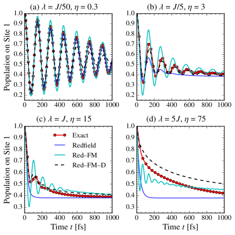
Figure 5: Comparison of numerically exact (HEOM) population dynamics to the results of standard Markovian Redfield theory, a straightforward variant of Markovian Redfield theory with frozen modes (Red–FM), and a dephasing–corrected variant as discussed in the text (Red–FM–D). The system–bath Hamiltonian is that of Ref. Ishizaki and Fleming, 2009a with $\varepsilon=100$ cm^-1, $J=100$ cm^-1, $\omega_{c}^{-1}=100$ fs, and $T=300$ K.

Appendix C RDM Hybrid Method

Here we relax the mode–freezing approximation by deriving a fully hybrid method that separates the complete system into a slow part consisting of the low–frequency component of the bath, and a rapidly–evolving part that includes both the electronic system and the high–frequency portion of the phonon bath. In this hybrid scheme, the slow part is treated quasi–classically, while the fast part is treated at the level of Redfield theory. Overall, the fast (slow) component of the system evolves in the mean field of the slow (fast) one.

Other hybrid approaches that combine classical and quantum dynamics include the self–consistent hybrid method of Wang and coworkers,Wang, Thoss, and Miller (2001); Thoss, Wang, and Miller (2001) which yields numerically exact dynamics, and the approximate hybrid–NIBA approach of Refs. Berkelbach, Reichman, and Markland, 2012; Berkelbach, Markland, and Reichman, 2012 In the former method, $\omega^{*}$, which is the energy scale that determines the splitting of the bath into slow and fast parts, is strictly a convergence parameter. In the latter, $\omega^{*}$ is an empirically determined adjustable parameter. As an approximate method, the hybrid–Redfield scheme derived here is akin to the hybrid–NIBA method. For a more detailed discussion of the hybrid RDM method, we refer the reader to Ref. Berkelbach, Reichman, and Markland, 2012.

As in the Redfield–FM approach, we make the approximation that $\Gamma(t)\approx\rho_{\mathrm{slow}}\rho_{\mathrm{sys+fast}}(t)$, where $\rho_{\mathrm{sys+fast}}(t)$ is the density matrix for the system and fast bath degrees of freedom and $\rho_{\mathrm{slow}}(t)$ is the density matrix for the slow bath degrees of freedom. The system and fast bath modes obey the following effective Liouville equation,

$$\frac{d\rho_{\mathrm{sys+fast}}(t)}{dt}=-i[H^{\prime\prime}(t),\rho_{\mathrm{sys+fast}}(t)],$$ (33)

where

$$\begin{split}H^{\prime\prime}(t)&=[\varepsilon+\lambda^{cl}(t)]\sigma_{z}+\Delta\sigma_{x}\\ &\hskip 10.00002pt+\sigma_{z}\sum_{k\in\text{fast}}c_{k}Q_{k}+\frac{1}{2}\sum_{k}\Big{[}P_{k}^{2}+\omega_{k}^{2}Q_{k}^{2}\Big{]},\end{split}$$ (34)

and $\lambda^{cl}$ is a dynamically fluctuating bias, $\lambda^{cl}(t)=\sum_{k\in\text{slow}}c_{k}Q_{k}(t)$.

A classical treatment of the reservoir leads to the following equations of motion,

$$\frac{dQ_{k}}{dt}=P_{k},$$ (35)

and

$$\begin{split}\frac{dP_{k}}{dt}&=-\omega_{k}^{2}Q_{k}-c_{k}\tilde{\sigma}_{z}(t).\end{split}$$ (36)

Employing the Ehrenfest approach demands that each part of the system evolves in the mean field of the other. For the quantum portion, the classical mean field consists of the time–dependent contribution to the bias, $\lambda^{cl}(t)$. For the classical portion, the force term $-c_{k}\tilde{\sigma}_{z}(t)=-c_{k}\operatorname{Tr}_{\mathrm{sys+fast}}[\sigma_{z}\rho_{\mathrm{sys+fast}}(t)]$ in the equations of motion embodies the mean–field ‘back–reaction.’ This force term moves the classical oscillators from the ground state minima to the displaced minima associated with the excited state.

Using Eqs. (5) and (34), the time–local Redfield equation takes the form

$$\begin{split}\frac{d}{dt}\rho(t)&=-i[H^{\prime\prime}_{\mathrm{sys}}(t),\rho(t)]\\ &\hskip 10.00002pt-\int_{0}^{t}ds\ \Big{\{}C(s)[\sigma_{z},\sigma_{z}(-s)\rho(t)]\\ &\hskip 50.00008pt-C^{*}(s)[\sigma_{z},\rho(t)\sigma_{z}(-s)]\Big{\}},\end{split}$$ (37)

where $\sigma_{z}(t)=U_{0}^{\dagger}(t)\sigma_{z}U_{0}(t)$, $U_{0}(t)=\exp[-i\int_{0}^{t}d\tau\ H_{\mathrm{sys}}^{\prime\prime}(\tau)]$, and $H_{\mathrm{sys}}^{\prime\prime}(t)=[\varepsilon+\lambda^{cl}(t)]\sigma_{z}+\Delta\sigma_{x}+\sum_{k\in\text{slow}}[P_{k}^{2}+\omega_{k}^{2}Q_{k}^{2}]/2$. The bath correlation, as in the case of the Redfield–FM method, takes the following form,

$$\begin{split}C(t)&=\frac{1}{\pi}\int_{0}^{\infty}d\omega\ J_{\mathrm{fast}}(\omega)\\ &\hskip 40.00006pt\times[\coth(\beta\omega/2)\cos(\omega t)-i\sin(\omega t)].\end{split}$$ (38)

To obtain the results shown in Fig. 3, trajectories corresponding to a set of initial conditions sampled from the Wigner distributionHillery et al. (1984) were calculated via a second–order Runge–Kutta scheme, using a step size of $\delta t=0.01\Delta^{-1}$. As required by the Runge–Kutta procedure, $\tilde{\sigma}_{z}(t)$ was kept constant during the evolution of the bath while $\lambda^{cl}(t)$ was kept constant during the evolution of the system. Explicitly, over a half–time step, the equations for the bath become

$$\begin{split}Q_{k}\left(t+\frac{\delta t}{2}\right)&=\alpha_{k}(t)\cos\left(\frac{\omega_{k}\delta t}{2}\right)-\frac{c_{k}}{\omega_{k}^{2}}\tilde{\sigma_{z}}(t)\\ &\hskip 10.00002pt+\frac{P_{k}(t)}{\omega_{k}}\cos\left(\frac{\omega_{k}\delta t}{2}\right),\end{split}$$ (39)

and

$$\begin{split}P_{k}\left(t+\frac{\delta t}{2}\right)&=P_{k}(t)\cos\left(\frac{\omega_{k}\delta t}{2}\right)+\omega_{k}\alpha_{k}(t)\sin\left(\frac{\omega_{k}\delta t}{2}\right),\end{split}$$ (40)

where

$$\alpha_{k}(t)=Q_{k}(t)+\frac{c_{k}}{\omega_{k}^{2}}\tilde{\sigma_{z}}(t).$$ (41)

In the hybrid–NIBA method of Ref. Berkelbach, Reichman, and Markland, 2012 the zeroth–order propagator necessary to evolve the perturbation in the interaction picture, $U_{0}(t)=\exp[-i\int_{0}^{\infty}d\tau H_{\mathrm{sys}}^{\prime\prime}(\tau)]$, was simple to calculate since $H_{\mathrm{sys}}^{\prime\prime}$ was diagonal. In contrast, $H_{\mathrm{sys}}^{\prime\prime}(t)$ for hybrid–Redfield contains off–diagonal elements. Within the Runge–Kutta scheme, this obstacle is easy to overcome, though it requires diagonalization of the time dependent $H_{\mathrm{sys}}^{\prime\prime}(t)$ at every time step. Because numerical diagonalization at every time–step is necessary for systems with more than two degrees of freedom, this can become computationally expensive for sufficiently large systems.

References

- Bloch (1957) F. Bloch, Phys. Rev. 105, 1206 (1957).
- Redfield (1965) A. G. Redfield, Adv. Magn. Reson. 1, 1 (1965).
- Nitzan (2006) A. Nitzan, Chemical Dynamics in Condensed Phases: Relaxation, Transfer, and Reactions in Condensed Molecular Systems (Oxford University Press, 2006).
- Ishizaki and Fleming (2009a) A. Ishizaki and G. R. Fleming, J. Chem. Phys. 130, 234110 (2009a).
- Weiss (1999) U. Weiss, Quantum Dissipative Systems, 2nd ed. (World Scientific, Singapore, 1999).
- Note (1) This criterion is only approximately valid because it ignores the magnitude of the system timescales. A more rigorous expression could be obtained via direct examination of the ratio of the 2nd and 4th order terms that may be found, e.g., in the work of Laird and SkinnerLaird1991 or Ref. \rev@citealpnumBreuerPetruccione.
- Landry and Subotnik (2015) B. R. Landry and J. E. Subotnik, J. Chem. Phys. 142, 104102 (2015).
- Berkelbach, Markland, and Reichman (2012) T. C. Berkelbach, T. E. Markland, and D. R. Reichman, J. Chem. Phys. 136, 084104 (2012).
- Berkelbach, Reichman, and Markland (2012) T. C. Berkelbach, D. R. Reichman, and T. E. Markland, J. Chem. Phys. 136, 034113 (2012).
- Thoss, Wang, and Miller (2001) M. Thoss, H. Wang, and W. H. Miller, J. Phys. Chem. 115, 2991 (2001).
- Craig and Manolopoulos (2005) I. R. Craig and D. E. Manolopoulos, J. Chem. Phys. 122, 84106 (2005).
- Stock (1995) G. Stock, J. Chem. Phys. 103, 2888 (1995).
- Breuer and Petruccione (2002) H.-P. Breuer and F. Petruccione, The Theory of Open Quantum Systems (Oxford University Press, 2002).
- Chang and Skinner (1993) T.-M. Chang and J. Skinner, Phys. A 193, 483 (1993).
- Zwanzig (1961) R. Zwanzig, Phys. Rev. 124, 983 (1961).
- Jang, Cao, and Silbey (2002) S. Jang, J. Cao, and R. J. Silbey, J. Chem. Phys. 116, 2705 (2002).
- Shibata and Arimitsu (1980) F. Shibata and T. Arimitsu, J. Phys. Soc. Jpn. 49, 891 (1980).
- Yoon, Deutch, and Freed (1975) B. Yoon, J. M. Deutch, and J. H. Freed, J. Chem. Phys. 62, 4687 (1975).
- Mukamel, Oppenheim, and Ross (1978) S. Mukamel, I. Oppenheim, and J. Ross, Phys. Rev. A 17, 1988 (1978).
- Breuer, Kappler, and Petruccione (1999) H. P. Breuer, B. Kappler, and F. Petruccione, Phys. Rev. A 59, 14 (1999).
- Coalson and Evans (2004) R. D. Coalson and D. G. Evans, Chem. Phys. 296, 117 (2004).
- Yang and Fleming (2002) M. Yang and G. R. Fleming, Chem. Phys. 275, 355 (2002).
- Palenberg et al. (2001) M. A. Palenberg, R. J. Silbey, C. Warns, and P. Reineker, J. Chem. Phys. 114, 4386 (2001).
- Pollard, Felts, and Friesner (1996) W. T. Pollard, A. K. Felts, and R. A. Friesner, in Advances in Chemical Physics: New Methods in Computational Quantum Mechanics, Volume 93, edited by I. Prigogine and S. A. Rice (John Wiley & Sons, Inc., 1996) p. 77.
- Ishizaki and Fleming (2009b) A. Ishizaki and G. R. Fleming, PNAS 106, 17255 (2009b).
- Wang, Thoss, and Miller (2001) H. Wang, M. Thoss, and W. H. Miller, J. Chem. Phys. 115, 2979 (2001).
- Hillery et al. (1984) M. Hillery, R. F. O’Connell, M. O. Scully, and E. P. Wigner, Phys. Rep. 106, 121 (1984).